A frustrated honeycomb-bilayer Heisenberg antiferromagnet: The spin-$\frac{1}{2}$ $J_{1}$–$J_{2}$–$J_{1}^{\perp}$ model

Abstract

We use the coupled cluster method to study the zero-temperature quantum phase diagram of the spin-$\frac{1}{2}$ $J_{1}$–$J_{2}$–$J_{1}^{\perp}$ model on the honeycomb bilayer lattice. In each layer we include both nearest-neighbor and frustrating next-nearest-neighbor antiferromagnetic exchange couplings, of strength $J_{1}>0$ and $J_{2}\equiv\kappa J_{1}>0$, respectively. The two layers are coupled by an interlayer nearest-neighbor exchange, with coupling constant $J_{1}^{\perp}\equiv\delta J_{1}>0$. We calculate directly in the infinite-lattice limit both the ground-state energy per spin and the Néel magnetic order parameter, as well as the triplet spin gap. By implementing the method to very high orders of approximation we obtain an accurate estimate for the full boundary of the Néel phase in the $\kappa\delta$ plane. For each value $\delta<\delta_{c}^{>}(0)\approx 1.70(5)$ we find an upper critical value $\kappa_{c}(\delta)$, such that Néel order is present for $\kappa<\kappa_{c}(\delta)$. Conversely, for each value $\kappa<\kappa_{c}(0)\approx 0.19(1)$ we find an upper critical value $\delta_{c}^{>}(\kappa)$, such that Néel order persists for $0<\delta<\delta_{c}^{>}(\kappa)$. Most interestingly, for values of $\kappa$ in the range $\kappa_{c}(0)<\kappa<\kappa^{>}\approx 0.215(2)$ we find a reentrant behavior such that Néel order exists only in the range $\delta_{c}^{<}(\kappa)<\delta<\delta_{c}^{>}(\kappa)$, with $\delta_{c}^{<}(\kappa)>0$. These latter upper and lower critical values coalesce when $\kappa=\kappa^{>}$, such that $\delta_{c}^{<}(\kappa^{>})=\delta_{c}^{>}(\kappa^{>})\approx 0.25(5)$.

I INTRODUCTION

Quantum magnets, comprising systems with a magnetic ion with spin quantum number $s$ sitting on each of the $(N\to\infty)$ sites of an extended regular periodic lattice, provide a rich playground for the study of quantum many-body systems with exotic ground-state (GS) phases that are entirely absent in their classical counterparts. These latter systems here correspond to precisely the same spin-lattice systems but in the limit where $s\to\infty$, such that the spins become classical. Of particular interest in this context is the often subtle interplay that ensues between frustration and quantum fluctuations. Frustration may be either geometrically induced [e.g., as on the two-dimensional (2D) triangular lattice] or dynamically induced. The latter is of special interest since it may be tuned.

Thus, for example, one may vary the relative strengths of competing interactions that are present in the model Hamiltonian under study, and which tend in the classical $(s\to\infty)$ case to frustrate one another in the sense that each interaction, in the absence of the other, tends to promote a different form of magnetic long-range order (LRO). As is well known, such forms of frustration often tend to promote the appearance of classical GS phases that are macroscopically degenerate in energy. For the quantum-mechanical counterparts (with a finite value of $s$), the quantum fluctuations present, due to the fact that any such stable classical GS phase is not an eigenstate of the quantum Hamiltonian, then act particularly strongly among the degenerate set of states. Such a scenario then offers enhanced possibilities for the complete suppression of quasiclassical magnetic LRO, with the associated emergence of such exotic states as various valence-bond crystalline (VBC) phases, multipolar or spin-nematic phases, and quantum spin-liquid (QSL) phases.

In broad terms quantum fluctuations tend to be stronger, other things being equal, for spin-lattice systems with lower values of each of the parameters (i) spatial dimensionality $d$, (ii) spin quantum number $s$, and (iii) lattice coordination number $z$. The Mermin-Wagner theorem Mermin and Wagner (1966) excludes all forms of magnetic LRO in any isotropic Heisenberg spin-lattice system with $d=1$, even at zero temperature $(T=0)$, or with $d=2$, except precisely at $T=0$. This is due to the fact that for any such system it is impossible to break a continuous symmetry. For this reason 2D spin-lattice models at $T=0$ now occupy a special arena in which to study quantum phase transitions. From among the eleven 2D Archimedean lattices, the honeycomb lattice is the simplest of the four that share the lowest value, $z=3$, of the coordination number. Of these four it is also the most commonly occurring in real quasi-2D magnetic materials. Frustrated spin-$\frac{1}{2}$ models on the 2D monolayer honeycomb lattice have hence become intensively studied in recent years Rastelli et al. (1979); Mattsson et al. (1994); Fouet et al. (2001); Mulder et al. (2010); Wang (2010); Cabra et al. (2011); Ganesh et al. (2011a); *Ganesh:2011_honey_errata_merge; Clark et al. (2011); Farnell et al. (2011); Reuther et al. (2011); Albuquerque et al. (2011); Mosadeq et al. (2011); Oitmaa and Singh (2011); Mezzacapo and Boninsegni (2012); Li et al. (2012a); Bishop et al. (2012); Bishop and Li (2012); Li et al. (2012b); Bishop et al. (2013); Ganesh et al. (2013); Zhu et al. (2013); Zhang and Lamas (2013); Gong et al. (2013); Yu et al. (2014). Much less work Zhao et al. (2012); Gong et al. (2015); Bishop and Li (2016); Li et al. (2016); Li and Bishop (2016) has been done on frustrated honeycomb-lattice monolayers comprising spins with $s\geq 1$.

The unfrustrated honeycomb-lattice Heisenberg antiferromagnet has isotropic nearest-neighbor (NN) exchange interactions only, all with equal strength $J_{1}>0$. The quantum fluctuations, that are present for all finite values of the spin quantum number $s$, act to reduce partially the perfect Néel LRO present on the bipartite lattice in the classical $(s\to\infty)$ limit. Nevertheless, they do not destroy it completely for any value of $s$ Li et al. (2016), even for the lowest value $s=\frac{1}{2}$. Instead, the Néel sublattice magnetization $M$ is fractionally reduced in a monotonically increasing fashion as $s$ is reduced. However, even for $s=\frac{1}{2}$, the Néel order parameter $M$ takes a value equal to about 54% of its classical limiting value (see, e.g., Refs. Oitmaa et al. (1992); Löw (2009); Jiang (2012); Farnell et al. (2014); Bishop et al. (2015)). Hence, to destroy the Néel LRO in the honeycomb monolayer requires the addition of frustrating interactions. Perhaps the simplest way to do so is to include isotropic antiferromagnetic (AFM) Heisenberg exchange interactions between next-nearest-neighbor (NNN) pairs of spins, all with equal strength $J_{2}>0$, resulting in the so-called $J_{1}$–$J_{2}$ model. The corresponding $J_{1}$–$J_{2}$–$J_{3}$ model also includes isotropic Heisenberg exchange interactions between next-next-nearest-neighbor (NNNN) pairs of spins with equal coupling strength $J_{3}$. The latter model has been studied particularly along the line $J_{3}=J_{2}$ that includes the point $J_{3}=J_{2}=\frac{1}{2}J_{1}$ of maximum classical frustration. The three classical phases that the model exhibits in the sector where $J_{i}>0$ $(i=1,2,3)$ all meet at this triple point, at which the classical GS phase is also macroscopically degenerate.

The spin-$\frac{1}{2}$ $J_{1}$–$J_{2}$–$J_{3}$ monolayer model, or special cases of it (especially those with $J_{3}=0$ or $J_{3}=J_{2}$), on the honeycomb lattice have been intensively investigated by a variety of theoretical techniques in recent years (see, e.g., Refs. Rastelli et al. (1979); Mattsson et al. (1994); Fouet et al. (2001); Mulder et al. (2010); Wang (2010); Cabra et al. (2011); Ganesh et al. (2011a); *Ganesh:2011_honey_errata_merge; Clark et al. (2011); Farnell et al. (2011); Reuther et al. (2011); Albuquerque et al. (2011); Mosadeq et al. (2011); Oitmaa and Singh (2011); Mezzacapo and Boninsegni (2012); Li et al. (2012a); Bishop et al. (2012); Bishop and Li (2012); Li et al. (2012b); Bishop et al. (2013); Ganesh et al. (2013); Zhu et al. (2013); Zhang and Lamas (2013); Gong et al. (2013); Yu et al. (2014)). Although some open unsettled questions do still remain, nevertheless by now there is a considerable degree of consensus about its overall $T=0$ quantum phase diagram, as discussed more fully in Sec. II. By contrast, much less attention has been devoted to analogous bilayer models (see, e.g., Refs. Ganesh et al. (2011a); *Ganesh:2011_honey_errata_merge; Ganesh et al. (2011c); Oitmaa and Singh (2012); Zhang et al. (2014); Arlego et al. (2014); Gómez Albarracín and Rosales (2016); Zhang et al. (2016)), even in the unfrustrated monolayer case where $J_{3}=J_{2}=0$, and even though some experimentally studied quasi-2D materials with a honeycomb-lattice structure are well modeled as honeycomb bilayers. A prime example is the bismuth oxynitrate layered material Bi₃Mn₄O₁₂(NO₃) Smirnova et al. (2009); Okubo et al. (2010), in which the spin-$\frac{3}{2}$ Mn⁴⁺ ions are ordered in honeycomb layers with no appreciable distortion. More precisely, the crystal field of the MnO₆ octahedral complexes, combined with a strong Hund’s rule coupling, leads in this compound to Heisenberg-like moments on the Mn⁴⁺ ions with an effective value $s=\frac{3}{2}$ for the spin quantum number. Two layers of such Mn⁴⁺ honeycomb lattices are separated in Bi₃Mn₄O₁₂(NO₃) by bismuth atoms. The resulting bilayers are themselves well separated spatially in this compound, and it seems therefore to be a good approximation to take the bilayer honeycomb lattice as the relevant model in which to describe its magnetic properties and behavior. It has also been suggested that a corresponding experimental realization of a spin-$\frac{1}{2}$ Heisenberg model on the honeycomb bilayer could be obtained by substituting V⁴⁺ ions in place of the Mn⁴⁺ ions in Bi₃Mn₄O₁₂(NO₃).

Thus, both for potential experimental reasons and theoretically, since the addition of an interlayer exchange coupling is another way of destroying the Néel order in honeycomb-lattice monolayers with NN interactions only, it is undoubtedly of interest to study Heisenberg models on honeycomb-lattice bilayers, in which competing frustration on top of the NN intralayer AFM exchange couplings $J_{1}$ is present due both to NNN intralayer AFM exchange couplings $J_{2}$ and to NN interlayer AFM exchange couplings $J_{1}^{\perp}$. We shall study the resulting $J_{1}$–$J_{2}$–$J_{1}^{\perp}$ model here for the case $s=\frac{1}{2}$. Since the coupled cluster method (CCM) has already been applied to the $s=\frac{1}{2}$ $J_{1}$–$J_{2}$–$J_{3}$ Heisenberg model on the honeycomb monolayer (or to special cases of it, e.g., with $J_{3}=J_{2}$ or $J_{3}=0$) with great success Farnell et al. (2011); Li et al. (2012a); Bishop et al. (2012); Bishop and Li (2012); Li et al. (2012b); Bishop et al. (2013), and where it has been shown to give a good description of the $T=0$ phase diagram of the model, including estimates for its quantum critical points (QCPs) which are among the best currently available, we also use the method here.

We note from the outset that the spin-$\frac{1}{2}$ $J_{1}$–$J_{2}$–$J_{1}^{\perp}$ model on the bilayer honeycomb lattice has also been studied recently Zhang et al. (2014); Arlego et al. (2014) using a Schwinger-boson parametrization of the spin operators followed by a mean-field decoupling. The results obtained for the model by this Schwinger-boson mean field theory approach were also augmented by, and compared with, corresponding results from both the exact diagonalization of a small (24-site) cluster and a dimer-series expansion calculation carried out to (the relatively low) fourth-order for the triplet spin energy gap Zhang et al. (2014); Arlego et al. (2014). It is thus of particular interest to compare our own results from a potentially much more accurate high-order implementation of the CCM with these earlier results. As a foretaste we note that while the two sets of results show many qualitative similarities (e.g., for the overall shape of the Néel phase boundary), significant quantitative differences are also found, as discussed more fully in Sec. V.

In Sec. II we first describe the model itself, including a description of the salient features of the limiting case, $J_{1}^{\perp}=0$, of the monolayer model. We then briefly describe the main elements of the CCM in Sec. III, before presenting our results in Sec. IV. We conclude with a discussion and summary in Sec. V.

II THE MODEL

The Hamiltonian of the $J_{1}$–$J_{2}$–$J_{1}^{\perp}$ model on the honeycomb bilayer lattice is given by

$$H= J_{1}\sum_{{\langle i,j\rangle},\alpha}\mathbf{s}_{i,\alpha}\cdot\mathbf{s}_{j,\alpha}+J_{2}\sum_{{\langle\langle i,k\rangle\rangle},\alpha}\mathbf{s}_{i,\alpha}\cdot\mathbf{s}_{k,\alpha}$$ (1)

$$+J_{1}^{\perp}\sum_{i}\mathbf{s}_{i,A}\cdot\mathbf{s}_{i,B}\,,$$

where the index $\alpha=A,B$ denotes the two layers, and where each site $i$ of the honeycomb lattice on each of the two layers carries a spin-$s$ particle described by the SU(2) spin operator ${\bf s}_{i,\alpha}\equiv(s^{x}_{i,\alpha},s^{y}_{i,\alpha},s^{z}_{i,\alpha})$, with ${\bf s}^{2}_{i,\alpha}=s(s+1)$. For the case considered here, $s=\frac{1}{2}$. The sums over $\langle i,j\rangle$ and $\langle\langle i,k\rangle\rangle$ in Eq. (1) run over all intralayer NN and NNN bonds, respectively, on each honeycomb-lattice monolayer, counting each pairs of spins once and once only in each of the two sums. The last sum in Eq. (1) over the index $i$ thus includes all NN interlayer pairs. We shall be interested here in the case when all three bonds are AFM in nature. With no loss of generality we may henceforth put $J_{1}\equiv 1$ to set the overall energy scale. The (monolayer) honeycomb lattice is non-Bravais with two sites per unit cell. It comprises two interlacing triangular Bravais sublattices, shown by filled and empty circles respectively in Fig. 1. The honeycomb bilayer lattice thus has four sites per unit cell, also as shown in Fig. 1.

 

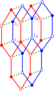
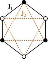
Figure 1: The $J_{1}$–$J_{2}$–$J_{1}^{\perp}$ model on the honeycomb bilayer lattice, showing (a) the two layers $A$ (red) and $B$ (blue), the nearest-neighbor bonds ($J_{1}=$ —–; $J_{1}^{\perp}=$ - - -), and the four sites ($1_{A},2_{A},1_{B},2_{B}$) of the unit cell; and (b) the intralayer bonds $J_{1}=$ —–; $J_{2}=$ - - -) on each layer. Sites on the two monolayer triangular sublattices are shown by filled and empty circles respectively.

In order to set the scene for our later discussion of the AFM honeycomb bilayer lattice, we first comment on the situation for the corresponding monolayer lattice (i.e., when $J_{1}^{\perp}=0$). In this case the classical ($s\to\infty$) $J_{1}$–$J_{2}$ model on the honeycomb lattice has Néel order (i.e., where all of the spins on the lattice sites denoted by filled circles in Fig. 1 point in a given, arbitrary, direction, and those on the sites denoted by empty circles point in the opposite direction) for all values $0\leq J_{2}/J_{1}\leq\frac{1}{6}$ of the intralayer frustration parameter. For values $J_{2}/J_{1}>\frac{1}{6}$ the classical monolayer spins acquire spiral order Rastelli et al. (1979); Fouet et al. (2001). In fact the spiral wave vector of the corresponding GS phase can point in an arbitrary direction and there exists an infinite one-parameter family of states, all of which are degenerate in energy. It has been shown that at the level of lowest-order spin-wave theory, in which the leading correction in the parameter $1/s$ is considered, this accidental degeneracy is then lifted by spin-wave fluctuations, so that particular spiral wave vectors are favored, thereby leading to so-called spiral order by disorder Mulder et al. (2010).

In more detail, in the region $\frac{1}{6}\leq J_{2}/J_{1}\leq\frac{1}{2}$ two distinct spiral phases, called the spiral-I and spiral-II phases, coexist, while for $J_{2}/J_{1}>\frac{1}{2}$ the stable GS phase comprises only the spiral-I phase Rastelli et al. (1979); Fouet et al. (2001). In fact, for the larger classical $J_{1}$–$J_{2}$–$J_{3}$ model on the honeycomb monolayer, the two points $(J_{2}/J_{1},J_{3}/J_{1})=(\frac{1}{6},0),(\frac{1}{2},0)$ are tricritical points Fouet et al. (2001). At the former point the two spiral phases meet the Néel phase, while at the latter point they meet another collinear AFM phase, called the Néel-II phase, described below. More generally, in the classical limit $(s\to\infty)$, there exists an infinitely degenerate family of noncoplanar states, all of whom are degenerate in energy with the Néel-II states, for every pair of values of the exchange coupling constants $J_{2}/J_{1}$ and $J_{3}/J_{1}$ for which the Néel-II state exists as a stable GS phase. It has been shown Fouet et al. (2001) that both thermal and quantum fluctuations then favor the collinear Néel-II AFM phase, thereby lifting the otherwise accidental degeneracy at the fully classical level.

Just like the Néel phase, the Néel-II phase also consists of sets of parallel zigzag (or sawtooth) AFM chains along one of the three equivalent honeycomb directions. However, whereas NN spins on adjacent chains are also antiparallel for the Néel state, for the Néel-II state they are parallel. Hence, equivalently, the Néel and Néel-II states have, respectively, all 3 and 2 NN pairs of spins aligned antiparallel to one another. There are thus three equivalent Néel-II states, one each corresponding to one of the three fundamental honeycomb-lattice directions. Each has a four-sublattice (i.e., a 4-site unit cell) structure, and each clearly breaks the lattice rotational symmetry, unlike the Néel state.

For the corresponding quantum versions of the $J_{1}$–$J_{2}$ honeycomb-lattice model (i.e., with finite values of the spin quantum number $s$), it is to be expected that quantum fluctuations will act to destroy the spiral order that is present in the classical $(s\to\infty)$ case for $J_{2}/J_{1}\geq\frac{1}{6}$. For the case $s=\frac{1}{2}$ there is wide consensus via a variety of theoretical calculational schemes that this indeed is the case. It has been shown by the CCM technique used here, for example, that for the spin-$\frac{1}{2}$ case spiral order is absent over the entire range $0\leq J_{2}/J_{1}\leq 1$ Bishop et al. (2012, 2013). It is also to be expected, a priori, that since quantum fluctuations generally tend to favor collinear order, the critical value of $J_{2}/J_{1}$ above which Néel order melts in the spin-$\frac{1}{2}$ $J_{1}$–$J_{2}$ model on the honeycomb lattice will be greater than the classical value of $\frac{1}{6}$. A large variety of different calculations now concurs with this expectation, giving a corresponding critical value for the $s=\frac{1}{2}$ case of about 0.2 (see, e.g., Refs. Albuquerque et al. (2011); Mosadeq et al. (2011); Mezzacapo and Boninsegni (2012); Bishop et al. (2012, 2013); Ganesh et al. (2013); Zhu et al. (2013); Zhang and Lamas (2013); Gong et al. (2013); Yu et al. (2014)). The CCM technique, which we employ here, for example, yields a critical value for $J_{2}/J_{1}$ of 0.207(3) for the QCP above which Néel order vanishes.

Turning now to the corresponding $J_{1}$–$J_{2}$–$J_{1}^{\perp}$ honeycomb-lattice bilayer model, it is clear that at the classical $(s\to\infty)$ level, the introduction of the NN interlayer coupling $J_{1}^{\perp}$ is basically trivial. Since it introduces no additional frustration into the system, the classical Néel phase (and the spiral phases) are completely unaffected. All that happens is that the NN interlayer pairs simply anti-align (for the case $J_{1}^{\perp}>0$ considered here). However, for the quantum versions of the model (with the spin quantum number $s$ taking a discrete finite value) the situation is more complicated and more interesting. Thus, for example, when the NN interlayer coupling $J_{1}^{\perp}$ is large enough to dominate the intralayer NN and NNN couplings, $J_{1}$ and $J_{2}$, respectively, one clearly expects the GS phase to be an interlayer dimer VBC (IDVBC) phase, with NN spins across the two layers forming independent spin-zero dimers. Since the energy of each such dimer is $-\frac{3}{4}J_{1}^{\perp}$ for our spin-$\frac{1}{2}$ model, we expect the GS energy per spin for the bilayer system in this limit to be given by

$$\frac{E}{N}\xrightarrow[J_{1}^{\perp}\to\infty]{}\frac{E^{{\rm IDVBC}}}{N}=-\frac{3}{8}J_{1}^{\perp}\,.$$ (2)

Whereas the Néel state, and all other quasiclassical states with magnetic LRO, are gapless, since their basic excitations are Goldstone magnon modes, the IDVBC state will be gapped. The breaking of a single spin-zero interlayer dimer to form a spin-1 NN pair is the lowest-lying excited state for the IDVBC state, and hence we expect the triplet spin gap in this limit to be given by

$$\Delta\xrightarrow[J_{1}^{\perp}\to\infty]{}\Delta^{{\rm IDVBC}}=J_{1}^{\perp}\,.$$ (3)

Thus, in the $J_{1}$–$J_{2}$–$J_{1}^{\perp}$ model on the honeycomb lattice, there are two different ways to destabilize the Néel LRO. One can either increase the frustration on each layer by increasing the strength $J_{2}$ of the NNN intralayer AFM interaction, or increase the strength $J_{1}^{\perp}$ of the NN interlayer AFM coupling. While the effect of the former for the extreme quantum case, $s=\frac{1}{2}$, has been much studied, as discussed above, the effect of the latter has received much less attention. It is our intention here to apply to this model the same method, namely the CCM, as has previously been applied to the model in the absence of interlayer coupling $(J_{1}^{\perp}=0)$ with considerable success.

III THE COUPLED CLUSTER METHOD

The CCM has been successfully applied to a wide variety of quantum many-body systems Farnell and Bishop (2004); Bishop and Kümmel (1987); Bishop (1991, 1998), including a large number of spin-lattice models in quantum magnetism (and see, e.g., Refs. Li et al. (2012a); Bishop et al. (2012); Bishop and Li (2012); Li et al. (2012b); Bishop et al. (2013); Bishop and Li (2016); Li et al. (2016); Li and Bishop (2016); Farnell et al. (2014); Bishop et al. (2015); Farnell and Bishop (2004); Zeng et al. (1998); Bishop et al. (2000); Krüger et al. (2000); Farnell et al. (2001); Darradi et al. (2005); Bishop et al. (2008a, b, 2009, 2010a, 2010b); Bishop and Li (2011); Li and Bishop (2012); Li et al. (2012c). The method affords a well-structured computational framework in which to study a variety of candidate GS phases and their actual regimes of stability. The description in each case is capable of systematic improvement via well-defined computational hierarchies of approximations for the multispin quantum correlations incorporated. We now describe briefly the main elements and the key features of the CCM, and refer the interested reader to the extensive literature (and see, e.g., Refs. Farnell and Bishop (2004); Bishop and Kümmel (1987); Bishop (1991, 1998); Kümmel et al. (1978); Bishop and Lührmann (1978, 1982); Arponen (1983); Bartlett (1989); Arponen and Bishop (1991); Zeng et al. (1998) and references cited therein) for further details.

The CCM is a size-extensive method, and automatically provides results in the limit of an infinitely large number of lattices spins, $N\rightarrow\infty$, at every level of approximation, as we shall see in more detail below. The method is implemented in practice by first choosing a suitable normalized reference (or model) state $|\Phi\rangle$, with respect to which the multiparticle correlations present in the exact GS wave function $|\Psi\rangle$ can be incorporated systematically to higher and higher orders of approximation as one approaches the (usually unattainable in practice) exact limit. As we shall see, the role of $|\Phi\rangle$ is that of a generalized vacuum state, broadly speaking. The exact GS ket wave function $|\Psi\rangle$ is chosen to satisfy the intermediate normalization condition, $\langle\Phi|\Psi\rangle=\langle\Phi|\Phi\rangle\equiv 1$, and its corresponding bra counterpart is defined as $\langle\tilde{\Psi}|\equiv\langle\Psi|/\langle\Psi|\Psi\rangle$, so that $\langle\tilde{\Psi}|\Psi\rangle=1$. For the present case $|\Phi\rangle$ will be chosen to be the quasiclassical AFM Néel state.

One of the defining features of the CCM is the specific way in which $|\Psi\rangle$ and $\langle\tilde{\Psi}|$ are now independently parametrized with respect to the model state $|\Phi\rangle$ in terms of two correlation operators $S$ and $\tilde{S}$ via the exponentiated forms,

$$|\Psi\rangle=e^{S}|\Phi\rangle\,;\quad\langle\tilde{\Psi}|=\langle\Phi|\tilde{S}e^{-S}\,,$$ (4)

that are characteristic of the method. Despite the fact that the destruction correlation operator $\tilde{S}$ may be expressed formally in terms of its creation counterpart $S$, by using Hermiticity, as

$$\langle\Phi|\tilde{S}=\frac{\langle\Phi|e^{S^{\dagger}}e^{S}}{\langle\Phi|e^{S^{\dagger}}e^{S}|\Phi\rangle}\,,$$ (5)

the choice is made within the CCM to treat $S$ and $\tilde{S}$ as independent operators, which will clearly satisfy Eq. (5) when no approximations are made, but which may violate this relation when truncations are made. They are formally decomposed as

$$S=\sum_{I\neq 0}{\cal{S}}_{I}C_{I}^{+}\,,\quad\tilde{S}=1+\sum_{I\neq 0}{\cal{\tilde{S}}}_{I}C_{I}^{-}\,,$$ (6)

where $C_{0}^{+}\equiv 1$ is defined to be the identity operator in the many-body Hilbert space, and where the set index $I$ denotes an appropriate complete set of single-particle configurations for all $N$ particles. The model state $|\Phi\rangle$ is thus required to be a cyclic (or fiducial) vector with respect to the set $\{C_{I}^{+}\}$ of mutually commuting many-body creation operators,

$$[C_{I}^{+},C_{J}^{+}]=0\,,\quad\forall I,J\neq 0\,,$$ (7)

such that the set of states $\{C_{I}^{+}|\Phi\rangle\}$ completely span the ket-state Hilbert space. Furthermore, we require that

$$\langle\Phi|C_{I}^{+}=0=C_{I}^{-}|\Phi\rangle\,,\quad\forall I\neq 0\,,$$ (8)

where $C_{I}^{-}\equiv(C_{I}^{+})^{\dagger}$ is the respective multiconfigurational destruction operator. It is also convenient in practice to choose the set of states $\{C_{I}^{+}|\Phi\rangle\}$ to be orthonormal,

$$\langle\Phi|C_{I}^{-}C_{J}^{+}|\Phi\rangle=\delta(I,J)\,,\quad\forall I,J\neq 0\,,$$ (9)

where $\delta(I,J)$ is a generalized Kronecker symbol.

Some important consequences immediately flow from the general CCM parametrization of Eqs. (4), (6)–(8). Firstly, while explicit Hermiticity is not maintained within the CCM, a balancing feature is that the Goldstone linked cluster theorem is preserved, both in the exact formalism and at all levels of approximation when truncations are made to some subset of the set-indices $I$ in the decompositions of the correlation operators $S$ and $\tilde{S}$ expressed in Eq. (6), the proof of which we outline below. As a consequence, size-extensivity is preserved in all orders of approximation, and all thermodynamically extensive variables such as the GS energy are guaranteed to scale linearly with particle number $N$. Thus, in the CCM we work from the outset in the thermodynamic (or bulk) limit, $N\rightarrow\infty$. Hence, there is never any need for any finite-size scaling of our results, as is required in many alternative techniques. Secondly, the exponentiated forms of the CCM parametrizations of Eq. (4) also similarly guarantee the exact preservation of the important Hellmann-Feynman theorem at all levels of approximate implementation of the method. This feature guarantees self-consistency among the results for the physical parameters calculated at the same given level of approximation.

Clearly, from Eqs. (4) and (6), a knowledge of the CCM $c$-number coefficients $\{{\cal S}_{I},{\cal\tilde{S}}_{I}\}$ suffices to determine the GS expectation value of any physical operator. In turn, these coefficients are formally determined from minimizing the GS energy expectation functional,

$$\bar{H}=\bar{H}({\cal S}_{I},{\cal\tilde{S}}_{I})\equiv\langle\Phi|\tilde{S}e^{-S}He^{S}|\Phi\rangle\,,$$ (10)

from Eq. (4), with respect to each of the parameters $\{{\cal S}_{I},\tilde{{\cal S}}_{I};\forall I\neq 0\}$. Extremization of $\bar{H}$ with respect to the coefficient $\tilde{{\cal S}}_{I}$ from Eq. (6) trivially yields the necessary condition

$$\langle\Phi|C_{I}^{-}e^{-S}He^{S}|\Phi\rangle=0\,,\quad\forall I\neq 0\,.$$ (11)

Equation (11) is manifestly a coupled set of nonlinear equations for the set of GS ket-state coefficients $\{{\cal S}_{I}\}$. Formally, there are as many equations in the set as there are unknown parameters. Similarly, extremization of $\bar{H}$ from Eq. (10) with respect to the coefficient ${\cal S}_{I}$ from Eq. (6), leads to the corresponding set of coupled linear equations for the GS bra-state coefficients $\{\tilde{{\cal S}}_{I}\}$,

$$\langle\Phi|\tilde{S}e^{-S}[H,C_{I}^{+}]e^{S}|\Phi\rangle=0\,,\quad\forall I\neq 0\,.$$ (12)

Again, once the coefficients $\{{\cal S}_{I}\}$ have been obtained from solving Eq. (11), they can be used as input to Eq. (12), which again formally comprises the same number of (now linear) equations as unknown parameters $\{\tilde{{\cal S}}_{I}\}$.

Once Eq. (11) is satisfied, the GS energy $E$ is simply given as the value of $\bar{H}$ from Eq. (10) at the minimum, namely

$$E=\langle\Phi|e^{-S}He^{S}|\Phi\rangle=\langle\Phi|He^{S}|\Phi\rangle\,,$$ (13)

where, in the latter equation, we have also used Eqs. (6) and (8). Equation (12) may also be written in the equivalent form

$$\langle\Phi|\tilde{S}(e^{-S}He^{S}-E)C_{I}^{+}|\Phi\rangle=0\,,\quad\forall I\neq 0\,,$$ (14)

where we have made use of Eq. (13). Equation (14) then takes the explicit form of a set of generalized linear eigenvalue equations for the coefficients $\{\tilde{{\cal S}}_{I}\}$, once the coefficients $\{{\cal S}_{I}\}$ are assumed known, having been first obtained by solving Eq. (11).

Excited-state (ES) ket wave functions $|\Psi_{e}\rangle$ are now parametrized in the CCM in terms of an excitation operator

$$X^{e}=\sum_{I\neq 0}{\cal X}_{I}^{e}C_{I}^{+}\,,$$ (15)

employed linearly as

$$|\Psi_{e}\rangle=X^{e}e^{S}|\Phi\rangle\,.$$ (16)

By suitably combining the GS ket-state Schrödinger equation,

$$H|\Psi\rangle=E|\Psi\rangle\,;\quad\langle\tilde{\Psi}|H=E\langle\tilde{\Psi}|\,,$$ (17)

and its ES ket-state counterpart,

$$H|\Psi_{e}\rangle=E_{e}|\Psi_{e}\rangle\,,$$ (18)

we readily find the result

$$e^{-S}[H,X^{e}]e^{S}|\Phi\rangle=\Delta_{e}X^{e}|\Phi\rangle\,,$$ (19)

where we have used the fact that the operators $X^{e}$ and $S$ commute, due to their explicit defining forms in Eqs. (6) and (15), together with Eq. (7), and where $\Delta_{e}$ is defined to be the excitation energy,

$$\Delta_{e}=E_{e}-E\,.$$ (20)

The ES ket-state coefficients $\{{\cal X}_{I}^{e}\}$ and the excitation energy $\Delta_{e}$ may then be found from solving the corresponding set of equations

$$\langle\Phi|C_{I}^{-}[e^{-S}He^{S},X^{e}]|\Phi\rangle=\Delta_{e}{\cal X}_{I}^{e}\,,\quad\forall I\neq 0\,,$$ (21)

which is readily obtained by taking the overlap of Eq. (19) with the state $\langle\Phi|C_{I}^{-}$, and using both Eqs. (7) and (9) together with the previous observation that the operators $X^{e}$ and $S$ commute. Equation (21) again takes the form of a set of generalized linear eigenvalue equations.

It is interesting to note at this point that the exponential terms $e^{\pm S}$ that are a hallmark of the CCM GS and ES wave function parametrizations, always actually enter the equations that need to be solved for the CCM coefficients $\{{\cal S}_{I},{\tilde{\cal S}}_{I}\}$ and $\{{\cal X}_{I}^{e}\}$ only in the specific form of the similarity transform $e^{-S}He^{S}$ of the system Hamiltonian, as may be seen explicitly from Eqs. (11), (14), and (21). This may be expanded as the nested commutator sum,

$$e^{-S}He^{S}=\sum_{n=0}^{\infty}\frac{1}{n!}[H,S]_{n}\,,$$ (22)

where the $n$-fold nested commutator $[H,S]_{n}$ is defined iteratively for all integers $n\geq 0$ as

$$[H,S]_{n}\equiv[[H,S]_{n-1},S]\,;\quad[H,S]_{0}=H\,.$$ (23)

A further key feature of the CCM parametrization of Eqs. (4) and (6) is that the infinite sum in Eq. (22) will generally, in any practical implementation of the method, actually terminate (as here) at some low finite order. The reasons for this are due to the facts that the Hamiltonian $H$ usually (as in the present case) contains only finite-order multinomial terms in the corresponding set of single-particle operators, and that all of the elements of $S$ in its decomposition of Eq. (6) mutually commute, as in Eq. (7). Thus, for example, if $H$ involves no more than $m$-body interaction terms, its second-quantized form will contain terms with no more than $2m$ single-particle creation and annihilation operators. As a consequence the sum in Eq. (22) then terminates exactly at the term $n=2m$, with all higher-order terms vanishing identically.

Similarly, in the present case we note that our Hamiltonian expressed by Eq. (1) is bilinear in the SU(2) spin operators $(s_{k}^{x},s_{k}^{y},s_{k}^{z})$. We shall describe below in detail how in this case the operators $\{C_{I}^{+}\}$ are constructed as products of single spin-raising operators, $s_{k}^{+}\equiv s_{k}^{x}+is_{k}^{y}$, on various lattice sites $k$. The SU(2) commutation relations then immediately imply that the sum in Eq. (22) terminates at the term with $n=2$ for this case, with all nested commutators with $n\geq 2$ vanishing identically.

Another consequence of the required mutual commutativity relation of Eq. (7) between any pair of operators from the set $\{C_{I}^{+}\}$ is that all non-vanishing terms in the expansion of Eq. (22) for the similarity transform $e^{-S}He^{S}$ of the Hamiltonian must be linked to the Hamiltonians. Unlinked terms simply cannot arise due to Eq. (7), even when any truncation is made for the operator $S$ by curtailing the set-indices $I$ retained in the expansion of Eq. (6) to some selected subset. Hence, the CCM is bound by construction to preserve the Goldstone linked-cluster theorem (and its corollary of size extensivity) at any level of practical implementation, as already alluded to above.

From our previous discussion it is thus clear that the sole approximation that is needed to implement the CCM in practice is to restrict the set of multiconfigurational set-indices $\{I\}$ that we retain in the expansions of Eqs. (6) and (15) for the GS coefficients $\{{\cal S}_{I},\tilde{{\cal S}}_{I}\}$ and ES coefficients $\{{\cal X}_{I}^{e}\}$, respectively, to some manageable (finite or infinite) subset. Any such choice of approximation will depend on the particular model being studied and, especially, on the chosen model state $|\Phi\rangle$ and the associated set of creation operators $\{C_{I}^{+}\}$. We thus describe now how such choices can be made both for general spin-lattice models and, more particularly, for the present bilayer model.

For an arbitrary quantum spin-lattice system a particularly simple choice of model state $|\Phi\rangle$ is a quasiclassical independent-spin product state. All such states are characterized by an independent specification of the projection of the spin on every lattice site, along some given quantization axis (which may itself vary from site to site). The collinear AFM Néel state for the present bilayer model, in which all of the spins on sites denoted by filled circles in Fig. 1(a) point in a given (arbitrary) direction, and all those on sites denoted by open circles point in the opposing direction, is an example of such an independent-spin product state. It will be precisely our choice of model state for the GS results presented in Sec. IV. More generally, any quasiclassical state with perfect magnetic LRO offers a similar choice for a CCM GS model state. It is convenient to treat all such states in the same way. One simple way to do so is to make a passive rotation of each spin independently (i.e., by choosing suitable local spin quantization axes on each lattice site independently), such that every spin points in the same direction, say downwards (i.e., along the negative $z_{s}$ direction). All lattice sites thus become equivalent to one another, and all such independent-spin product states take the universal form $|\Phi\rangle=|\downarrow\downarrow\downarrow\cdots\downarrow\rangle$ in their own local sets of spin quantization axes. At the same time such rotations are clearly just unitary spin transformations that leave the basic SU(2) commutation relations unaltered. The big advantage, however, is that once such local frames are selected, all that needs to be done to distinguish one case from another is to rewrite the model Hamiltonian $H$ in terms of the specific choice made.

With such a choice of local spin axes, it is evident that $|\Phi\rangle$ is a fiducial vector with respect to a set of mutually commuting creation operators $\{C_{I}^{+}\}$ that are chosen to be products of single-spin raising operators $s_{k}^{+}$. More specifically, we choose $C_{I}^{+}\rightarrow s_{k_{1}}^{+}s_{k_{2}}^{+}\cdots s_{k_{n}}^{+};\,n=1,2,\cdots,2sN$, where $s$ is the spin quantum number ($=\frac{1}{2}$, for the present model) of all $N$ spins. The multiconfigurational set-index $I$ correspondingly becomes a set of lattice-site indices, $I\rightarrow\{k_{1},k_{2},\cdots,k_{n};\,n=1,2,\cdots,2sN\}$, wherein any given site index $k_{i}$ may appear up to $2s$ times.

We shall employ here a rather general and systematic approximation scheme for the choice of which configurations $\{I\}$ to retain in the sums in Eq. (6) for the decompositions of the CCM GS correlation operators $\{{\cal S},\tilde{\cal S}\}$, which has proven to be very powerful in many previous applications to a diverse array of spin-lattice models. This is the so-called localized (lattice-animal-based subsystem) LSUB$n$ scheme. At the $n$th level of approximation it retains all such multispin configurations that describe clusters of spins spanning a range of no more than $n$ contiguous lattice sites. Contiguity of a set of lattice sites is defined so that every site in the set is NN to at least one other in the set (in some specified geometry). Equivalently, in the LSUB$n$ scheme, the configurations retained are those defined on all possible lattice animals (or polyominos) up to size $n$. Clearly as the truncation parameter grows without bound ($n\rightarrow\infty$) the corresponding LSUB$\infty$ approximation becomes exact.

The effective size of the index set $\{I\}$ retained at a given LSUB$n$ level is reduced by making use of the space- and point-group symmetries of the lattice and the particular model state $|\Phi\rangle$ being used, as well as any pertinent conservation laws. For example, for the present model of Eq. (1) and the Néel model state, the total $z$-component of spin, $s_{T}^{z}\equiv\sum_{k=1}^{N}s_{k}^{z}$, is conserved (i.e., $s_{T}^{z}=0$ for the Néel state), where global spin axes are assumed. Even so, the number $N_{f}=N_{f}(n)$ of distinct (and nonzero) fundamental multispin-flip configurations that are retained at a given $n$th level of LSUB$n$ approximation grows rapidly (typically, super-exponentially) with the truncation index $n$. For example, for the spin-$\frac{1}{2}$ honeycomb monolayer, we have $N_{f}(10)=6\,237$ and $N_{f}(12)=103\,097$ for the Néel GS. By contrast, for the present spin-$\frac{1}{2}$ honeycomb bilayer, $N_{f}(10)=70\,118$.

For the ES calculation of the triplet spin gap, $\Delta$, the set of LSUB$n$ multispin-flip cluster configurations $\{I\}$ retained in the decomposition of Eq. (15) for excitation operator $X^{e}$ is, of course, different to that retained in the corresponding decompositions of Eq. (6) for the GS correlation operators $(S,\tilde{S})$ at the same $n$th level of approximation. Thus, for the calculation of the triplet spin gap based on the Néel state as CCM model state we now retain only those configurations $I$ that have $s_{T}^{z}=1$, compared to those that have $s_{T}^{z}=0$ for the AFM GS calculation. Nevertheless, both sets of GS and ES calculations are preformed within the same LSUB$n$ scheme for consistency and to assure comparable levels of accuracy in both. We note that at a given LSUB$n$ level of approximation, based on the same Néel model state, the number $N_{f}(n)$ of fundamental CCM configurations is higher for the ES calculation than for the GS calculation. For example, for the spin-$\frac{1}{2}$ honeycomb monolayer we have $N_{f}(10)=10\,497$ and $N_{f}(12)=182\,714$ for the spin triplet ES, whereas for the corresponding bilayer case we have $N_{f}(10)=121\,103$.

The derivation and solution of such large sets of equations clearly require the use of both massive parallelization and supercomputing resources. Their derivation Zeng et al. (1998) also requires the use of purpose-built, customized computer algebra packages ccm . Whereas for the spin-$\frac{1}{2}$ honeycomb-lattice monolayer we were able to perform LSUB$n$ calculations for the spin-$\frac{1}{2}$ $J_{1}$–$J_{2}$ model with $n\leq 12$ Bishop et al. (2012, 2013), for the corresponding present $J_{1}$–$J_{2}$–$J_{1}^{\perp}$ bilayer model we are only able to perform LSUB$n$ calculations with $n\leq 10$, due to the substantially increased numbers $N_{f}(n)$ of fundamental configurations in this case, as illustrated above.

Whereas the GS energy $E$ can, uniquely, be calculated from a knowledge of the CCM creation coefficients $\{{\cal S}_{I}\}$ alone, as from Eq. (13), any other GS quantity requires also a knowledge of the corresponding destruction coefficients $\{\tilde{{\cal S}}_{I}\}$. For example, we also calculate here the Néel magnetic order parameter $M$. This is defined to be the average on-site GS magnetization using the Néel state as the CCM model state $|\Phi\rangle$,

$$M=-\frac{1}{N}\sum_{k=1}^{N}\langle\Phi|\tilde{S}e^{-S}s_{k}^{z}e^{S}|\Phi\rangle\,,$$ (24)

in terms of the local rotated spin-coordinate frames described previously.

The last step in our CCM calculational procedure is to extrapolate the corresponding sequence of LSUB$n$ results for any GS or ES quantity that we have computed to the LSUB$\infty$ limit $(n\rightarrow\infty)$ in which all relevant multispin-flip configurations are retained, and the method hence becomes exact. From our previous description of the method it should be clear that this last step is the sole approximation made in the entire procedure. Despite the fact that, so far as we know, there exist no exact results for performing such extrapolations, a great deal of practical experience has by now been accumulated from the many applications of the CCM that have already been made to a wide variety of quantum spin-lattice systems. For example, for the GS energy per spin, $E/N$, there exists the highly accurate and very well tested extrapolation scheme (and see, e.g., Refs. Farnell et al. (2011); Li et al. (2012a); Bishop et al. (2012); Bishop and Li (2012); Li et al. (2012b); Bishop et al. (2013); Bishop and Li (2016); Li et al. (2016); Li and Bishop (2016); Farnell et al. (2014); Bishop et al. (2015); Farnell and Bishop (2004); Bishop et al. (2000); Krüger et al. (2000); Farnell et al. (2001); Darradi et al. (2005); Bishop et al. (2008a, b, 2009, 2010a, 2010b); Bishop and Li (2011); Li and Bishop (2012); Li et al. (2012c))

$$\frac{E(n)}{N}=e_{0}+e_{1}n^{-2}+e_{2}n^{-4}\,,$$ (25)

from fits to which we can obtain the LSUB$\infty$ value $e_{0}$. As one would expect a priori, the GS expectation values of other physical operators converge more slowly than does the energy [i.e., with leading exponents in their extrapolation schemes comparable to Eq. (25) that take values less than 2]. In particular, for the order parameter $M$ of Eq. (24), it has been well documented that the corresponding exponent depends sensitively on the degree of frustration present in the model. Not surprisingly perhaps, the exponent is smaller for situations with the highest frustration.

More explicitly, for models with only little or zero frustration, an extrapolation scheme for $M$ with a leading power $n^{-1}$ (i.e., with leading exponent equal to 1),

$$M(n)=m_{0}+m_{1}n^{-1}+m_{2}n^{-2}\,,$$ (26)

has been found to hold well and to give highly accurate results for many systems (and see, e.g., Refs. Li et al. (2012a); Bishop et al. (2012); Bishop and Li (2012); Bishop et al. (2013); Farnell et al. (2014); Bishop et al. (2000); Krüger et al. (2000); Farnell et al. (2001); Darradi et al. (2005); Bishop et al. (2009, 2010a, 2010b); Bishop and Li (2011)). Again from such a fit we obtain the extrapolated LSUB$\infty$ estimate $m_{0}$ for $M$. On the other hand, for systems that are close to a QCP, or for phases whose magnetic order parameter $M$ is either zero or very small, the scaling ansatz of Eq. (26) does not fit so well. A forced fit then tends to overestimate the correct LSUB$\infty$ extrapolant. As a consequence it also tends to predict a value for the critical strength of the frustrating interaction, which is responsible for driving the respective phase transition, that is too large. In such cases a more accurate scaling ansatz is always found to be (and see, e.g., Refs. Farnell et al. (2011); Li et al. (2012a); Bishop et al. (2012); Bishop and Li (2012); Li et al. (2012b); Bishop et al. (2013); Li et al. (2016); Li and Bishop (2016); Farnell et al. (2014); Bishop et al. (2008a, b); Li et al. (2012c))

$$M(n)=\mu_{0}+\mu_{1}n^{-1/2}+\mu_{2}n^{-3/2}\,,$$ (27)

from which $\mu_{0}$ gives the respective extrapolated LSUB$\infty$ value for $M$.

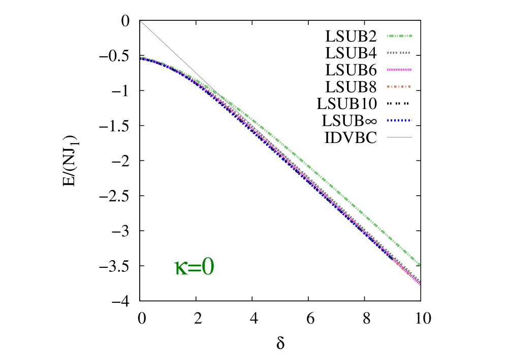
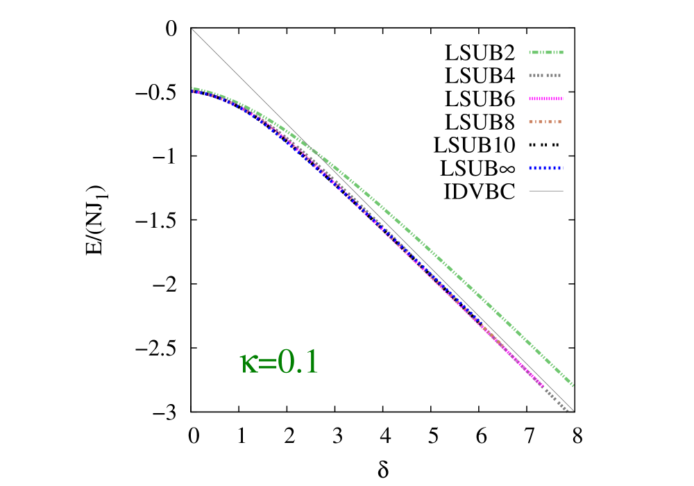
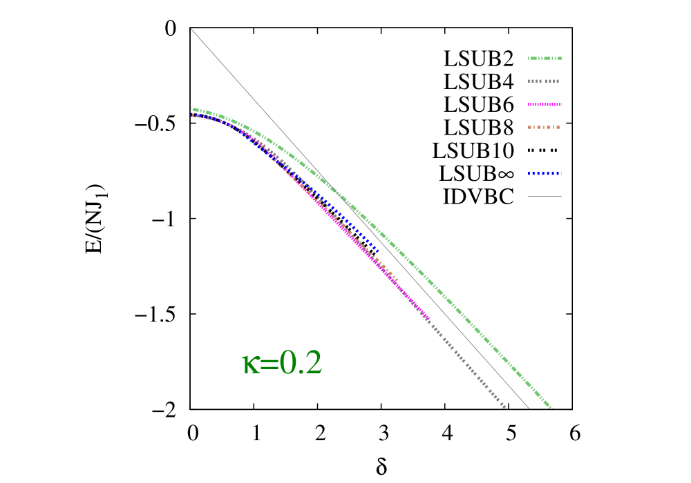
Figure 2: CCM results for the GS energy per spin $E/N$ (in units of $J_{1}$) versus the scaled interlayer exchange coupling constant, $\delta\equiv J_{1}^{\perp}/J_{1}$, for the spin-$\frac{1}{2}$ $J_{1}$–$J_{2}$–$J_{1}^{\perp}$ model on the bilayer honeycomb lattice (with $J_{1}>0$), for three selected values of the intralayer frustration parameter, $\kappa\equiv J_{2}/J_{1}$: (a) $\kappa=0$, (b) $\kappa=0.1$, and (c) $\kappa=0.2$. Results based on the Néel state as CCM model state are shown in LSUB$n$ approximations with $n=2,4,6,8,10$, together with the corresponding LSUB$\infty$ extrapolated results using Eq. (25) and the data sets $n=\{4,6,8,10\}$. For comparison, we also show the corresponding interlayer dimer VBC result of Eq. (2).

Finally, a CCM extrapolation scheme with a leading power of $n^{-1}$ has also been found to give an excellent fit to the LSUB$n$ results $\Delta(n)$ for the spin gap (and see, e.g., Refs. Li and Bishop (2016); Bishop et al. (2015); Krüger et al. (2000); Richter et al. (2015); Bishop and Li (2015)),

$$\Delta(n)=d_{0}+d_{1}n^{-1}+d_{2}n^{-2}\,,$$ (28)

from which the corresponding LSUB$\infty$ estimate $d_{0}$ for the spin gap $\Delta$ has been successfully extracted for a wide variety of spin-lattice models.

Clearly, to obtain robust fits, it is preferable to use at least four LSUB$n$ data points in using the extrapolation schemes of Eqs. (25)–(28), since each contains three fitting parameters. Occasionally this may be inappropriate for reasons we describe. In such cases it may also be suitable to use a wholly unbiased extrapolation scheme in which the leading exponent is itself also a fitting parameter. Thus, the LSUB$n$ approximants $P(n)$ for a physical parameter $P$ are then extrapolated to give the LSUB$\infty$ estimate $p_{0}$ via the unbiased scheme,

$$P(n)=p_{0}+p_{1}n^{-\nu}\,,$$ (29)

in which the three parameters $p_{0}$, $p_{1}$, and $\nu$ are all treated as quantities to be fitted.

Finally, we note that we may always perform an unbiased pre-fit of the form of Eq. (29) to any CCM LSUB$n$ sequence of results for an arbitrary physical parameter, whether or not four or more data points are available. In this way one may first check the (approximate) value of the exponent $\nu$, before using one of the above schemes of Eqs. (25)–(28), for example, which will almost always then lead to better extrapolated results due to the addition of the next-to-leading-order correction to the leading-order term. In practice, such a pre-fit to the results for the order parameter $M$ for example, essentially always leads to a clear choice between the fits of Eqs. (26) and (27). It is in this way that the extrapolation scheme for any physical parameter is matched in practice to a particular regime for the Hamiltonian under study.

IV RESULTS

We first show in Fig. 2 our results for the GS energy per spin as a function of the scaled interlayer exchange coupling constant, $\delta\equiv J_{1}^{\perp}/J_{1}$, for three different values of the interlayer frustration parameter, $\kappa\equiv J_{2}/J_{1}$. For each value of $\kappa$ we display the results based on the Néel state as CCM model state at LSUB$n$ approximation levels $n=2,4,6,8,10$. We also show the corresponding LSUB$\infty$ extrapolated values ($e_{0}/J_{1}$) obtained from using Eq. (25) together with the data sets $n=\{4,6,8,10\}$ as input. We see that in each case the convergence is extremely rapid as the truncation index $n$ is increased. We note too that, as is always the case in practical applications of the CCM, the LSUB$n$ results for all finite values of the truncation index $n$ extend beyond the actual Néel transition point out to some critical value beyond which no real solution to the CCM equations exists. As is also usually true, the natural termination point for the solution tracked for each LSUB$n$ set of GS equations, appears to converge uniformly as $n$ is increased to the corresponding QCP at which Néel order vanishes. These termination points for the GS CCM equations at each LSUB$n$ level of approximation are always direct manifestations of the respective QCP present in the physical system being studied, as has been well described and documented in many previous applications of the method (and see, e.g., Refs. Li et al. (2012a); Bishop et al. (2012, 2013); Farnell and Bishop (2004) and references cited therein). Furthermore, each CCM LSUB$n$ solution extends slightly into the unphysical regime, beyond the respective LSUB$\infty$ QCP, with the extent of the unphysical regime reducing monotonically to zero as the LSUB$n$ truncation index $n$ is increased to the exact $n\rightarrow\infty$ limit.

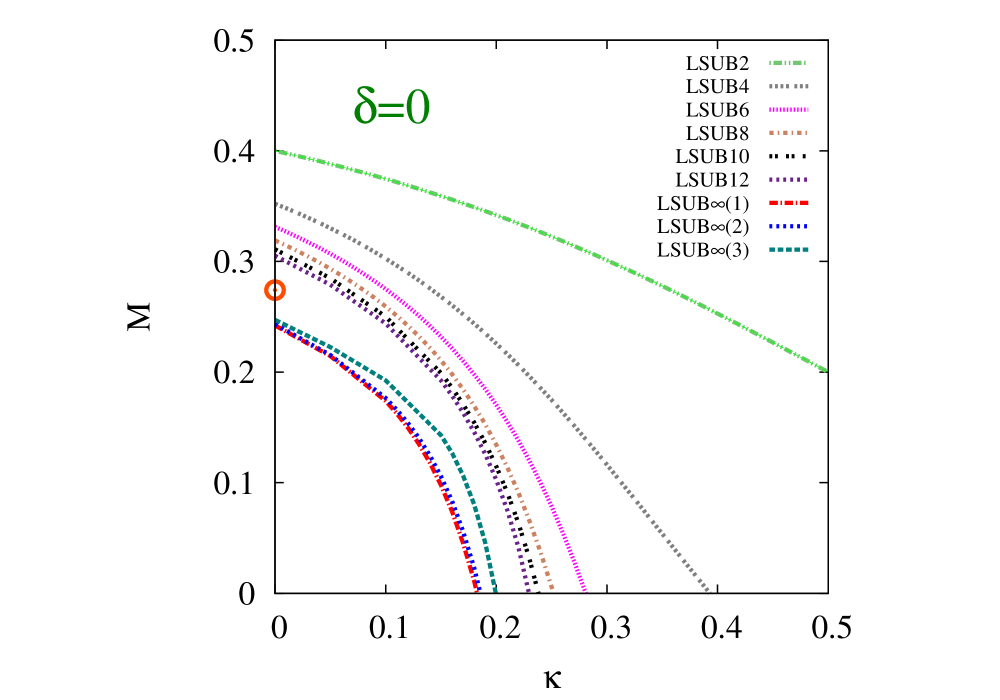
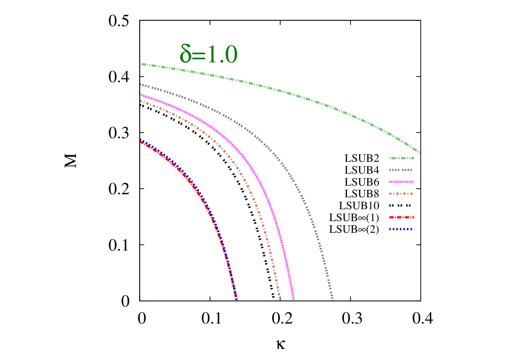
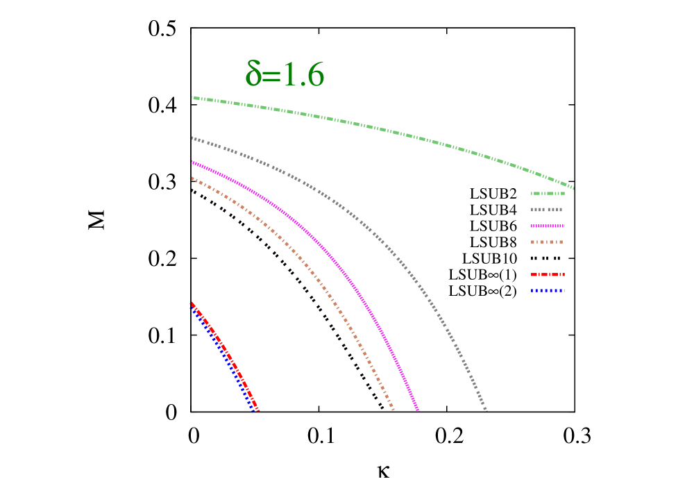
Figure 3: CCM results for the GS magnetic order parameter $M$ versus the intralayer frustration parameter, $\kappa\equiv J_{2}/J_{1}$, for the spin-$\frac{1}{2}$ $J_{1}$–$J_{2}$–$J_{1}^{\perp}$ model on the bilayer honeycomb lattice (with $J_{1}>0$), for three selected values of the scaled interlayer exchange coupling constant, $\delta\equiv J_{1}^{\perp}/J_{1}$: (a) $\delta=0$, (b) $\delta=1.0$, and (c) $\delta=1.6$. Results based on the Néel state as CCM model state are shown in LSUB$n$ approximations with $n=2,4,6,8,10$ (and also with $n=12$ for the special case of the $J_{1}$–$J_{2}$ monolayer, i.e., when $\delta=0$), together with various corresponding LSUB$\infty(i)$ extrapolated results using Eq. (27) and the respective data sets $n=\{2,6,10\}$ for $i=1$, $n=\{4,6,8,10\}$ for $i=2$, and $n=\{4,8,12\}$ for $i=3$ (for the case $\delta=0$ only). In Fig. 3(a), rather than crowd the figure with additional full curves based on (the largely inappropriate) Eq. (26), we show with the circle ($\bigcirc$) symbol the corresponding extrapolated value using Eq. (26) and the data set $n=\{4,6,8,10\}$ for the single point $\delta=0=\kappa$, where this extrapolation scheme is the appropriate one.

Before proceeding to our results for the magnetic order parameter and the triplet spin gap of the model, we pause to consider the accuracy of our results. One way to do so is the focus on the case $\delta=0=\kappa$ fo the pure spin-$\frac{1}{2}$ Heisenberg antiferromagnet (HAFM) on a honeycomb monolayer (i.e., with NN isotropic AFM Heisenberg exchange interactions only) since, for this unfrustrated case only, we may also compare our results with those of large-scale quantum Monte Carlo (QMC) simulations that are available. For this case, for example, our extrapolated LSUB$\infty$ results $e_{0}$ based on Eq. (25) are $E/N=-0.54473(2)J_{1}$ using the LUSB$n$ data set $n=\{4,6,8,10\}$, and $E/N=-0.54466(1)J_{1}$ using the corresponding set $n=\{6,8,10,12\}$. In both cases the errors cited are simply those associated with the respective fits. The two extrapolations are in clear good agreement with one another. They also agree extremely well with the result $E/N=-0.54455(2)J_{1}$ obtained from a large-scale, continuous Euclidean time QMC algorithm Löw (2009), and where this infinite-lattice result is based on extrapolating the QMC estimates for finite-sized $L\times L$ lattices with $16\leq L\leq 36$.

It has been observed previously Li and Bishop (2016) that for the $J_{1}$–$J_{2}$ model on the honeycomb monolayer (i.e., with $\delta=0$) there is a noticeable $(4m-2)/4m$ staggering effect in some of the CCM LSUB$n$ sequence of results. For example, in the spin-1 case this is even strong enough that for the Néel magnetic order parameter the corresponding curves with $n=4$ and $n=6$ actually cross one another at a value of the intralayer frustration parameter $\kappa\approx 0.2$. Clearly, in such cases, the two separate LSUB$n$ sequences of results (for a fixed value of $\kappa$) with $n=4m$ and $n=4m-2$, respectively, tend to converge differently from each other for all positive integral values of $m$, although both sequences themselves converge monotonically. To test for this effect here we have also extrapolated our results for the unfrustrated monolayer case (i.e., with $\kappa=0=\delta$) separately for the two sequences, since in this case alone are we also able to perform LSUB12 calculations. For the GS energy per spin for this case we obtain $E/N=-0.55473J_{1}$ using Eq. (25) with the LSUB$n$ data set $n=\{2,6,10\}$, and $E/N=-0.55468J_{1}$ with the corresponding set $n=\{4,8,12\}$. The level of agreement is again excellent.

We turn next to our results for the magnetic order parameter $M$ for the Néel state. Firstly, we show in Fig. 3(a) results for the case of the spin-$\frac{1}{2}$ honeycomb-lattice monolayer (i.e., with $\delta=0$), as a function of the intralayer frustration parameter $\kappa\equiv J_{2}/J_{1}$. In this case alone we are able to perform CCM LSUB$n$ calculations up to values $n=12$ of the truncation parameter, and hence we can again investigate whether the $(4m-2)/4m$ staggering effect is appreciable in our LSUB$n$ results for $M$. While the effect is not immediately evident in the pattern of the raw LSUB$n$ data, some effect is noticeable in the extrapolated results, particularly near the critical point at which the Néel LRO vanishes (i.e., where $M\rightarrow 0$).

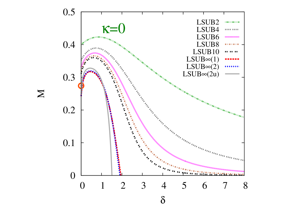
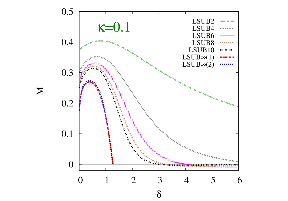
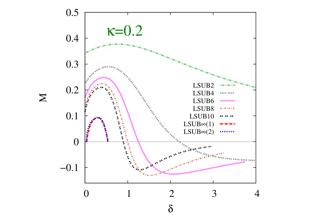
Figure 4: CCM results for the GS magnetic order parameter $M$ versus the scaled interlayer exchange coupling constant, $\delta\equiv J_{1}^{\perp}/J_{1}$, for the spin-$\frac{1}{2}$ $J_{1}$–$J_{2}$–$J_{1}^{\perp}$ model on the bilayer honeycomb lattice (with $J_{1}>0$), for three selected values of the intralayer frustration parameter, $\kappa\equiv J_{2}/J_{1}$: (a) $\kappa=0$, (b) $\kappa=0.1$, and (c) $\kappa=0.2$. Results based on the Néel state as CCM model state are shown in LSUB$n$ approximations with $n=2,4,6,8,10$, together with two corresponding LSUB$\infty(i)$ extrapolated results using Eq. (27) and the respective data sets $n=\{2,6,10\}$ for $i=1$ and $n=\{4,6,8,10\}$ for $i=2$. In Fig. 4(a), we also show the corresponding LSUB$\infty(2u)$ extrapolated result based on the unbiased scheme of Eq. (29) and the data set $n=\{4,6,8,10\}$. Furthermore in Fig. 4(a), rather than crowd the figure with additional full curves based on (the largely inappropriate) Eq. (26), we show with the circle ($\bigcirc$) symbol the corresponding extrapolated value using Eq. (26) and the data set $n=\{4,6,8,10\}$ for the single point $\kappa=0=\delta$, where this extrapolation scheme is the appropriate one.

Thus, in Fig. 3(a) we show three separate LSUB$\infty$ extrapolations, all based on the scheme of Eq. (27), using the respective data sets $n=\{2,6,10\}$, $n=\{4,6,8,10\}$, and $n=\{4,8,12\}$. While the first two extrapolations agree very closely with one another over the whole range of values of the intralayer frustration parameter $\kappa$ for which $M>0$, the latter extrapolation does differ somewhat from the other two, particularly near the QCP at which $M\rightarrow 0$. While the extrapolation scheme of Eq. (27) is certainly appropriate for the case where the frustration is appreciable, particularly for systems that are close to a QCP, the scheme of Eq. (26) is valid for unfrustrated (or only slightly frustrated) systems, such as at the point $\delta=0=\kappa$, and we show by the circle ($\bigcirc$) symbol in Fig. 3(a) the value of $M$ at this point using Eq. (26) and the data set $n=\{4,6,8,10\}$. The value so obtained is $M=0.2741(1)$ where, again, the error is simply that associated with the fit. Corresponding values using Eq. (26) and other LSUB$n$ data set as input are $M=0.2729(5)$ using $n=\{6,8,10,12\}$, $M=0.2761$ using $n=\{2,6,10\}$, $M=0.2733$ using $n=\{4,8,12\}$, and $M=0.2715$ using $n=\{8,10,12\}$. There is clearly a small sensitivity to the data set used, which results in an overall error of about $0.5\%$ for the value obtainable. Once again, our CCM results may be compared with those from two separate QMC estimates that have been performed in this limiting unfrustrated case, namely, $M=0.2681(8)$ Löw (2009) and $M=0.26882(3)$ Jiang (2012). The agreement with our CCM results is again good.

The sensitivity of the extrapolated results for the order parameter $M$ is, however, greater for cases where frustration is present, as can clearly be observed from Fig. 3(a), particularly in the region near the critical point where Néel LRO melts. Thus, for the honeycomb monolayer (i.e., when $\delta=0$), the corresponding LSUB$\infty$ estimates for the point $\kappa_{c}$ at which $M\rightarrow 0$, all based on the extrapolation scheme of Eq. (27) but with different LSUB$n$ data sets as input are, for example, $\kappa_{c}=0.183$ using $n=\{2,6,10\}$ and $\kappa_{c}=0.186$ based on $n=\{4,6,8,10\}$. However, inclusion of the LSUB12 results gives somewhat higher estimates. For example, we find $\kappa_{c}=0.207$ based on LSUB$n$ results with $n=\{6,8,10,12\}$, $\kappa_{c}=0.200$ based on $n=\{4,8,12\}$, and $\kappa_{c}=0.204$ based on $n=\{8,10,12\}$. Clearly, in this case, our estimates for $\kappa_{c}$ have an associated overall error of around $5\%$.

Corresponding results to those shown for the monolayer $(\delta=0)$ in Fig. 3(a) are shown in Figs. 3(b) and 3(c) for the bilayer for the two cases $\delta=1.0$ and $\delta=1.6$. It is evident that the critical value, $\kappa_{c}(\delta)$, at which Néel LRO melts, decreases as the strength $\delta\equiv J_{1}^{\perp}/J_{1}$ of the interlayer coupling increases, at least for values of $\delta$ above some lower critical value. We return to this point later. The effect of the interlayer coupling is also shown separately in Fig. 4 for three different values of the intralayer frustration parameter, $\kappa\equiv J_{2}/J_{1}$. Firstly, in Fig. 4(a), we show our CCM LSUB$n$ results with $n\leq 10$ for the Néel order parameter $M$ for the case of zero intralayer frustration (i.e., $\kappa=0$), where only NN interactions are present. Interestingly, as $\delta$ is first increased from zero, the effect of interlayer AFM NN coupling is to increase the order parameter $M$, and hence to enhance the stability of Néel LRO. The effect reaches a maximum at each level of approximation at a value $\delta\approx 0.5$. Once $\delta$ is increased further, however, Néel order begins to reduce, and in each LSUB$n$ approximation shown the order parameter $M$ tends to zero asymptotically as $\delta$ continues to increase. The relative shapes of the LSUB$n$ curves is particularly interesting, with clear evidence that as the truncation index $n$ is increased the asymptotic vanishing of the order parameter becomes appreciably sharper.

We also show in Fig. 4(a) two corresponding LSUB$\infty$ extrapolations for $M$, both based on the scheme of Eq. (27), but using respective LSUB$n$ data sets with $n=\{2,6,10\}$ and $n=\{4,6,8,10\}$ as input. Both extrapolations agree with each other very closely, with the corresponding estimates for the point $\delta_{c}^{>}$ at which $M\rightarrow 0$ being $\delta_{c}^{>}=1.944$ based on the set $n=\{2,6,10\}$, and $\delta_{c}^{>}=1.902$ based on the set $n=\{4,6,8,10\}$. We also show for comparison purposes in Fig. 4(a) the corresponding extrapolated result based on the unbiased scheme of Eq. (29), and using the LSUB$n$ data set $n=\{4,6,8,10\}$ as input, denoted as the LSUB$\infty(2u)$ curve. The overall level of agreement between the corresponding LSUB$\infty(2)$ and LSUB$\infty(2u)$ extrapolations is reasonable. While it is excellent for smaller values of the scaled interlayer coupling constant, $0<\delta\lesssim 1$, there is a greater degree of divergence at larger values, $\delta\gtrsim 1$. For example, the LSUB$\infty(2u)$ extrapolation yields a value $\delta_{c}^{>}=1.510$, compared to the corresponding LSUB$\infty(2)$ value $\delta_{c}^{>}=1.902$, for the case $\kappa=0$. The true value for $\delta_{c}^{>}$ at $\kappa=0$ certainly lies between these two estimates. A more detailed analysis of all our results yields our best estimate as $\delta_{c}^{>}\approx 1.70(5)$. Part of the difference clearly comes from the fact that Eq. (29) retains only the leading-order correction to the large-$n$ limit, while Eq. (27) also retains both the leading and sub-leading corrections. Nevertheless, it is likely that the scheme of Eq. (27) does somewhat overestimate the critical value $\delta_{c}^{>}$ in this case $\kappa=0$ when frustration is absent. We note that this level of discrepancy between the two different extrapolation schemes diminishes rapidly as intralayer frustration is introduced, such that for values $\kappa\gtrsim 0.1$ it seems to be negligible.

In Figs. 4(b) and 4(c) we also show comparable results to those for the unfrustrated $(\kappa=0)$ case shown in Fig. 4(a), for the two cases where the intralayer frustration parameter, $\kappa\equiv J_{2}/J_{1}$, takes the values $\kappa=0.1$ and $\kappa=0.2$, respectively. As expected, the effect of increasing frustration is observed generally to reduce the Néel order parameter $M$ at any given value of the interlayer coupling strength $\delta$. Accordingly, the upper critical value, $\delta_{c}^{>}(\kappa)$, of the interlayer coupling strength, above which Néel order vanishes, is seen to decrease monotonically as $\kappa$ is increased. Exactly as for the case $\kappa=0$ shown in Fig. 4(a), the two LSUB$\infty$ extrapolations for $M$ based on the scheme of Eq. (27), but with the two different LSUB$n$ data sets with $n=\{2,6,10\}$ and $n=\{4,6,8,10\}$, agree extremely closely with one another for all values of $\kappa$, with the agreement generally even improving as $\kappa$ is increased. For example, the values for $\delta_{c}^{>}(\kappa)$ at the values $\kappa=0.1$ and $\kappa=0.2$ shown in Figs. 4(b) and 4(c) obtained from the two separate LSUB$\infty$ extrapolations are $\delta_{c}^{>}(0.1)=1.275$, $\delta_{c}^{>}(0.2)=0.538$ based on the LSUB$n$ data set with $n=\{2,6,10\}$, and $\delta_{c}^{>}(0.1)=1.265$, $\delta_{c}^{>}(0.2)=0.535$ based on the respective set with$n=\{4,6,8,10\}$.

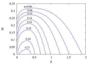
Figure 5: CCM results for the GS magnetic order parameter $M$ versus the scaled interlayer exchange coupling constant, $\delta\equiv J_{1}^{\perp}/J_{1}$, for the spin-$\frac{1}{2}$ $J_{1}$–$J_{2}$–$J_{1}^{\perp}$ model on the bilayer honeycomb lattice (with $J_{1}>0$), for a variety of values of the intralayer frustration parameter, $\kappa\equiv J_{2}/J_{1}$. In each case we show extrapolated results, based on the Néel state as CCM model state, obtained from using Eq. (27) with the corresponding LSUB$n$ data sets $n=\{4,6,8,10\}$.

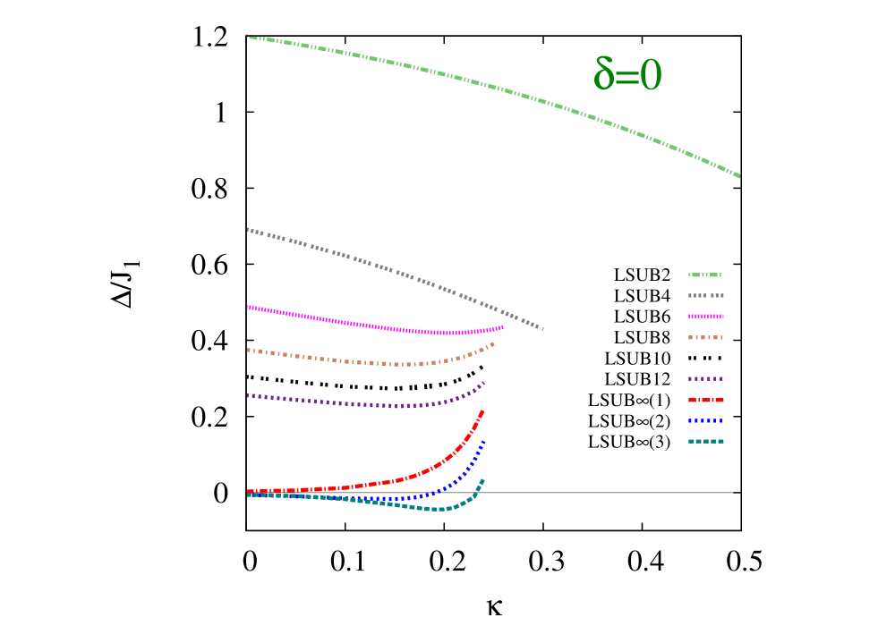
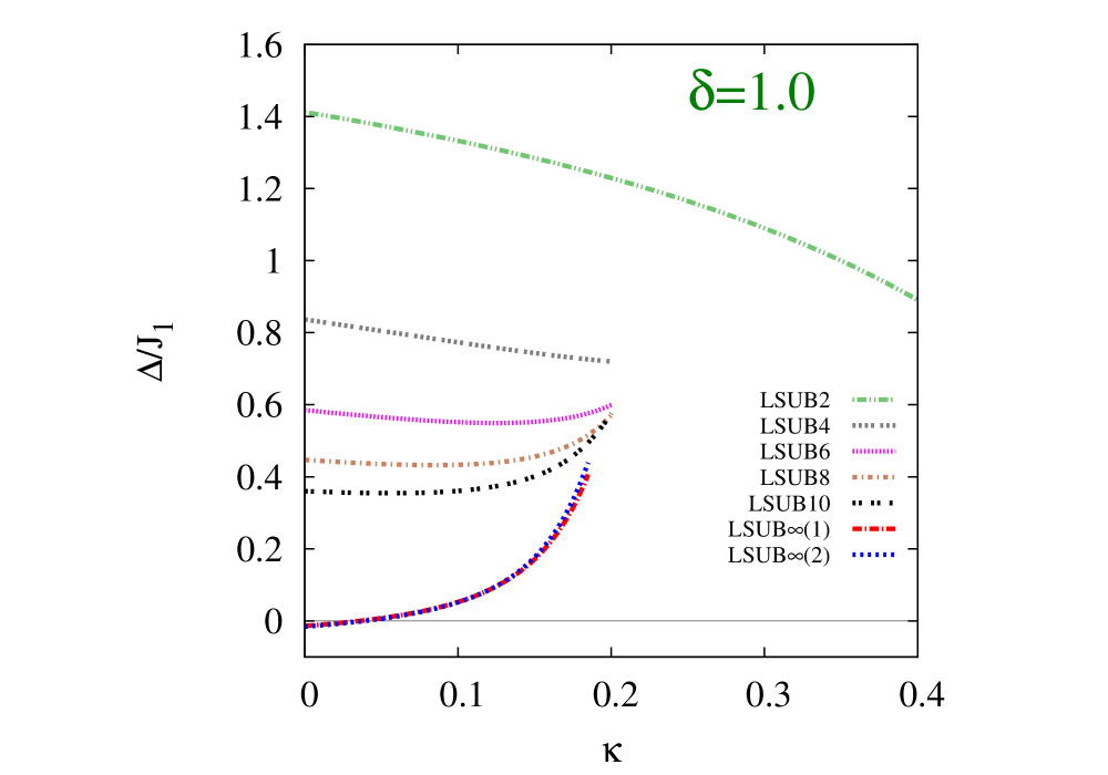
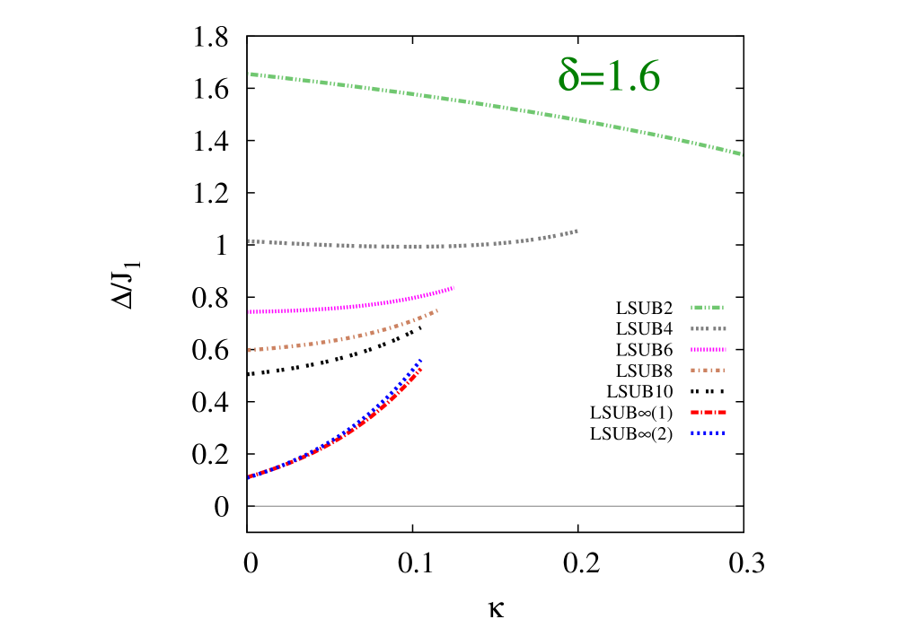
Figure 6: CCM results for the triplet spin gap $\Delta$ (in units of $J_{1}$) versus the intralayer frustration parameter, $\kappa\equiv J_{2}/J_{1}$, for the spin-$\frac{1}{2}$ $J_{1}$–$J_{2}$–$J_{1}^{\perp}$ model on the bilayer honeycomb lattice (with $J_{1}>0$), for three selected values of the scaled interlayer exchange coupling constant, $\delta\equiv J_{1}^{\perp}/J_{1}$: (a) $\delta=0$, (b) $\delta=1.0$, and (c) $\delta=1.6$. Results based on the Néel state as CCM model state are shown in LSUB$n$ approximations with $n=2,4,6,8,10$ (and also with $n=12$ for the special case of the $J_{1}$–$J_{2}$ monolayer, i.e., when $\delta=0$), together with various corresponding LSUB$\infty(i)$ extrapolated results using Eq. (28) and the respective data sets $n=\{2,6,10\}$ for $i=1$, $n=\{4,6,8,10\}$ for $i=2$, and $n=\{4,8,12\}$ for $i=3$ (for the case $\delta=0$ only).

In Fig. 4(c) the value $\kappa=0.2$ for which the order parameter $M$ is shown as a function of $\delta$ is greater than the above-quoted values $\kappa_{c}(0)$ above which Néel order vanishes in the monolayer $(\delta=0)$, for both LSUB$\infty$ extrapolations displayed. Interestingly now, however, for values $\kappa>\kappa_{c}(0)$ that are not too large, as $\delta$ is increased above a lower critical value $\delta_{c}^{<}(\kappa)$, Néel order is re-established due to the interlayer AFM coupling, up to the respective upper critical value $\delta_{c}^{>}(\kappa)$. For the value $\kappa=0.2$ shown in Fig. 4(c), for example, we find that the values for $\delta_{c}^{<}(0.2)$ obtained from the two separate LSUB$\infty$ extrapolations shown are $\delta_{c}^{<}(0.2)=0.041$ based on the LSUB$n$ data set with $n=\{2,6,10\}$, and $\delta_{c}^{<}(0.2)=0.033$ based on that with $n=\{4,6,8,10\}$. This behavior is further illustrated in Fig. 5, from which we clearly observe that there exists some upper critical value $\kappa^{>}$ of the intralayer frustration parameter $\kappa$ at which $\delta_{c}^{<}(\kappa^{>})=\delta_{c}^{>}(\kappa^{>})$, and hence such that Néel order is absent for all values $\kappa>\kappa^{>}$, whatever the value of $\delta$. Our corresponding LSUB$\infty$ estimates for $\kappa^{>}$ are $\kappa^{>}=0.216$ based on the LSUB$n$ data set with $n=\{2,6,10\}$ and $\kappa^{>}=0.214$ based on the set with $n=\{4,6,8,10\}$.

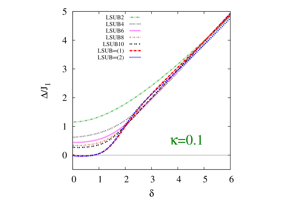
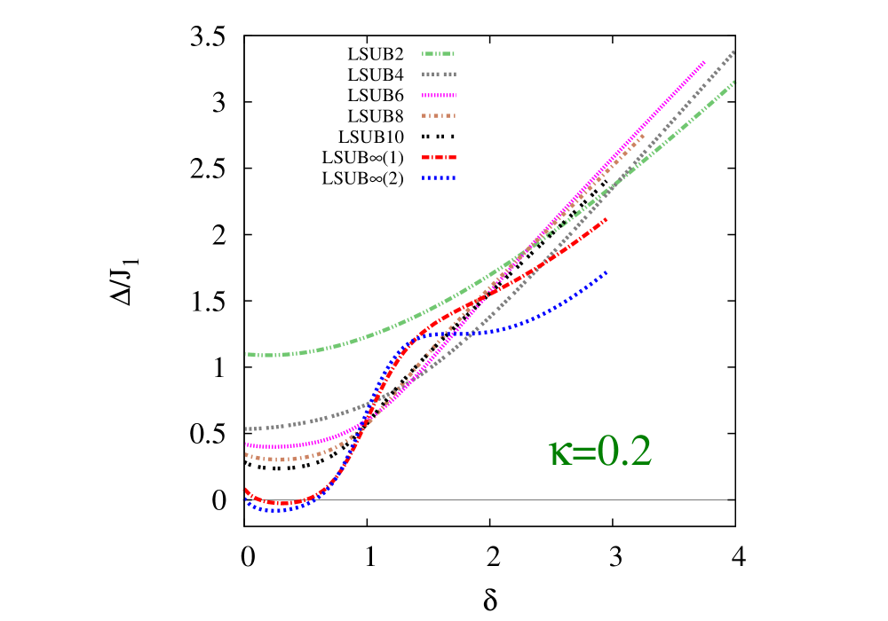
Figure 7: CCM results for the triplet spin gap $\Delta$ (in units of $J_{1}$) versus the scaled interlayer exchange coupling constant, $\delta\equiv J_{1}^{\perp}/J_{1}$, for the spin-$\frac{1}{2}$ $J_{1}$–$J_{2}$–$J_{1}^{\perp}$ model on the bilayer honeycomb lattice (with $J_{1}>0$), for three selected values of the intralayer frustration parameter, $\kappa\equiv J_{2}/J_{1}$: (a) $\kappa=0$, (b) $\kappa=0.1$, and (c) $\kappa=0.2$. Results based on the Néel state as CCM model state are shown in LSUB$n$ approximations with $n=2,4,6,8,10$, together with two corresponding LSUB$\infty(i)$ extrapolated results using Eq. (28) and the respective data sets $n=\{2,6,10\}$ for $i=1$ and $n=\{4,6,8,10\}$ for $i=2$.

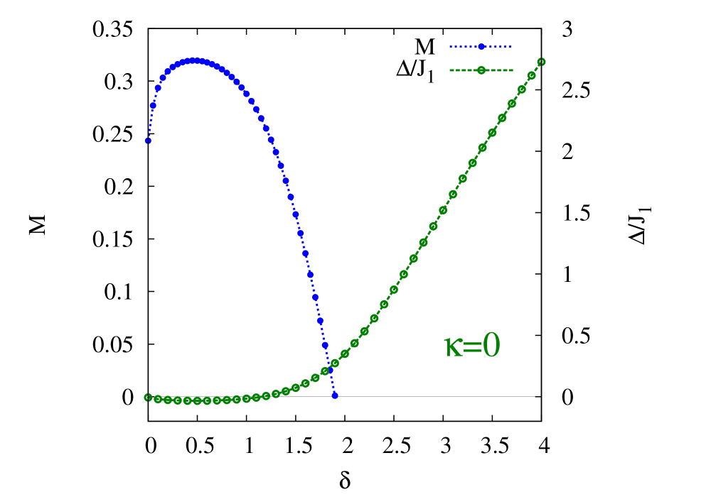
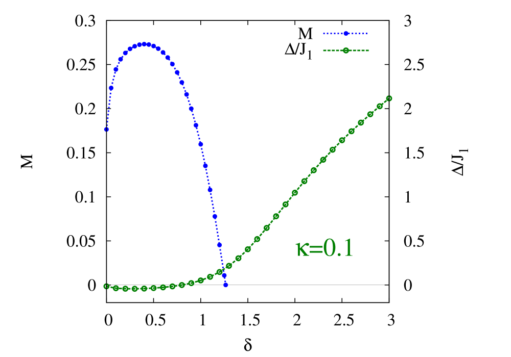
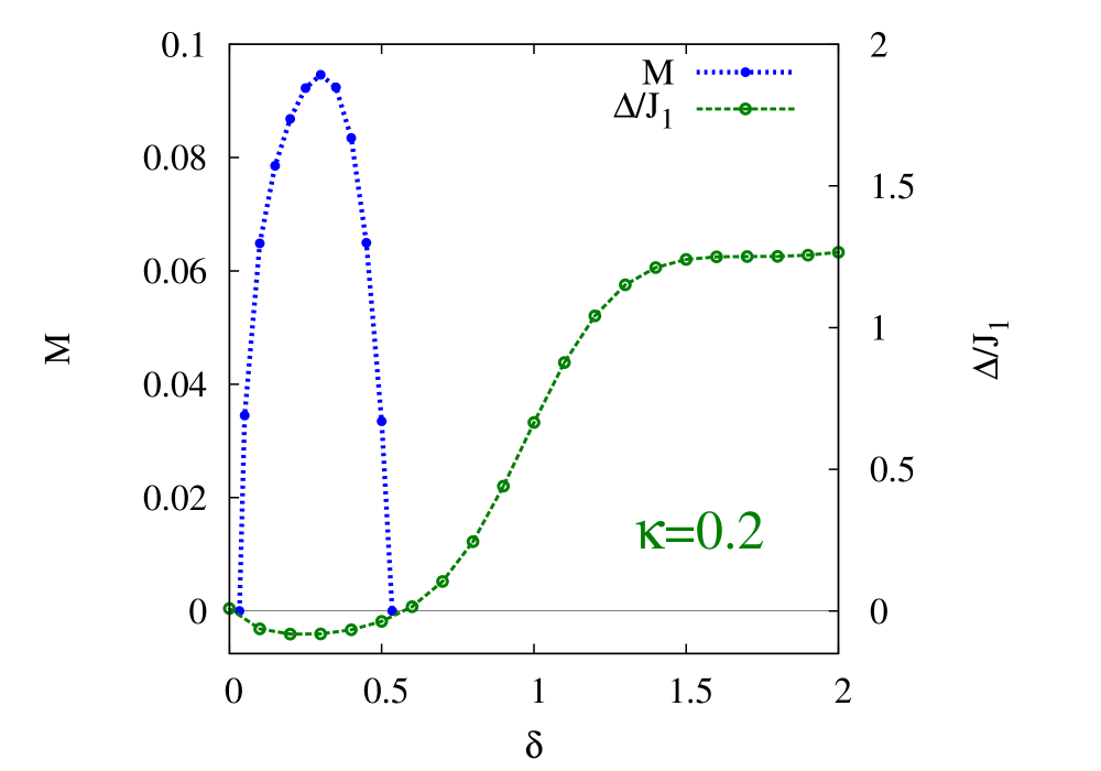
Figure 8: Juxtaposed CCM results for the magnetic order parameter $M$ (left scale) and the triplet spin gap $\Delta$ (in units of $J_{1}$, right scale) versus the scaled interlayer exchange coupling constant, $\delta\equiv J_{1}^{\perp}/J_{1}$, for the spin-$\frac{1}{2}$ $J_{1}$–$J_{2}$–$J_{1}^{\perp}$ model on the bilayer honeycomb lattice (with $J_{1}>0$), for three selected values of the intralayer frustration parameter, $\kappa\equiv J_{2}/J_{1}$: (a) $\kappa=0$, (b) $\kappa=0.1$, and (c) $\kappa=0.2$. Extrapolated results for $M$ and $\Delta$ are shown from using Eqs. (27) and (28), respectively, with the corresponding LSUB$n$ data sets with $n=\{4,6,8,10\}$ in each case, based on the Néel state as the CCM model state.

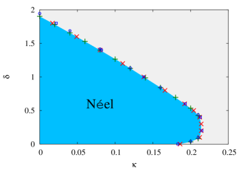
Figure 9: $T=0$ phase diagram of the spin-$\frac{1}{2}$ $J_{1}$–$J_{2}$–$J_{1}^{\perp}$ model on the bilayer honeycomb lattice with $J_{1}>0$, $\delta\equiv J_{1}^{\perp}/J_{1}$, and $\kappa\equiv J_{2}/J_{1}$. The darker (skyblue) region is the quasiclassical phase with AFM Néel order, while in the lighter (grey) region Néel order is absent. The red cross ($\times$) symbols and the green plus ($+$) symbols are points at which the extrapolated GS magnetic order parameter $M$ for the Néel phase vanishes, for specified values of $\delta$ and $\kappa$, respectively. They thus represent the values $\kappa_{c}(\delta)$ and $\delta_{c}^{>}(\kappa)$ [and also $\delta_{c}^{<}(\kappa)$ for values of $\kappa$ in the range $\kappa_{c}(0)<\kappa<\kappa^{>}$], respectively. In each case the Néel state is used as CCM model state, and Eq. (27) is used for the extrapolations with the corresponding LSUB$n$ data sets $n=\{4,6,8,10\}$. For comparison we also show by blue open square ($\square$) and open circle ($\bigcirc$) symbols respectively, some corresponding points obtained using the LSUB$n$ data set $n=\{2,6,10\}$.

We turn next to our corresponding results for the triplet spin gap $\Delta$. Firstly, we show in Fig. 6 corresponding sets of results as functions of $\kappa$ to those shown in Fig. 3 for the Néel magnetic order parameter $M$, for the same three fixed values of $\delta$. Figure 6(a) shows our LSUB$n$ results for the spin-$\frac{1}{2}$ honeycomb-lattice monolayer (i.e., with $\delta=0$), where again for this limiting case alone calculations are presented for values $n\leq 12$ of the LSUB$n$ truncation parameter. As before, in Fig. 3(a) for $M$, we now also show three separate LSUB$\infty$ extrapolations, based respectively on the LSUB$n$ data sets $n=\{2,6,10\}$, $n=\{4,6,8,10\}$, and $n=\{4,8,12\}$, and using the scheme of Eq. (28) in each case. It is evident that each of the extrapolations is consistent, within small numerical errors, with the gap being zero in the region $\kappa<\kappa_{c}(0)$ where Néel LRO is present, exactly as expected. There is also clear evidence that for values $\kappa>\kappa_{c}(0)$ the GS phase is gapped, consistent with it being a VBC state. Corresponding results for $\Delta=\Delta(\kappa)$ are shown in Fig. 6(b) and 6(c) for the bilayer with values $\delta=1.0$ and $\delta=1.6$ respectively of the interlayer coupling strength.

Once again, the effect of the interlayer coupling on the spin gap $\Delta$ is also displayed separately in Fig. 7 for the same three different values of the intralayer frustration parameter $\kappa$ as are shown in Fig. 4 for the Néel order parameter $M$. Figure 7(a) in particular clearly shows that $\Delta/J_{1}\rightarrow\delta$ in the large $\delta$ limit, exactly as expected for the IDVBC state, from Eq. (3). Each of the LSUB$\infty$ extrapolations shown gives results for the system being gapless over ranges of values of $\kappa$ that are in striking agreement with the ranges shown by the corresponding LSUB$\infty$ extrapolations in Fig. 4 for where Néel LRO survives. For the specific case $\kappa=0.2$ shown in Fig. 7(c), for example, there is clear evidence of both a lower critical value $\delta_{c}^{<}(0.2)$ and an upper critical value $\delta_{c}^{>}(0.2)$, between which the stable GS phase is gapless, and the values so obtained from the gap $\Delta$ are in excellent agreement with those values shown in Fig. 4(c) between which the Néel order parameter $M$ is nonzero. The overall level of agreement is shown even more clearly in Fig. 8, where our extrapolated CCM results for $M$ and $\Delta$ are juxtaposed on the same graph for the same three specific cases $\kappa=0$, $\kappa=0.1$, and $\kappa=0.2$. We note that the only significant disagreement between the values $\delta_{c}^{>}(\kappa)$ obtained from the extrapolations based on $M$ and $\Delta$ arises at $\kappa=0$. Here, as we have discussed previously, and shown in Fig. 4(a), it is likely that the extrapolation for $M$ based on Eq. (27) slightly overestimates the value $\delta_{c}^{>}(0)$. Correcting for this as we have indicated would thereby bring it into better agreement with the value obtained from $\Delta$.

We note that, within the CCM framework, the vanishing of the magnetic order parameter $M$ generally provides an appreciably more accurate estimate than the opening of a spin gap $\Delta$ for the critical coupling that marks the transition from a gapless state with quasiclassical magnetic LRO to a gapped non-magnetic state. The reason for this is that in most cases at the critical points where the (extrapolated) order parameter $M$ vanishes the slope of the curve for $M$ as a function of the respective coupling parameter is nonzero. This behavior is clearly seen here in Figs. 4 and 5, for example. By contract, the extrapolated curves for the spin gap $\Delta$ generally depart from being zero (at the same respective critical points) with zero slope, as one sees here from Figs. 6 and 7, for example. Correspondingly, the CCM estimates for the critical points have much larger errors than those obtained from the vanishing of $M$. What is interesting, however, is that if one assumes that the exact gap disappears at a critical point, as a function of the coupling, with non-zero (and possibly infinite) slope, a simple extrapolation of the CCM results in Fig. 7, for example, using values somewhat larger than the actual critical point (i.e., beyond where the curves shown start appreciably, and thence presumably artificially, to round) gives revised estimates for the critical points that are in remarkable closer agreement to those obtained from the vanishing of $M$. In this context we note that for the specific case $\kappa=0$ of the model with NN bonds only, the spin gap $\Delta$ has a singularity at the critical value $\delta_{c}^{>}(0)$ with a critical exponent $\nu$ given by the three-dimensional Heisenberg universal value $\nu\approx 0.71$ Le Guillou and Zinn-Justin (1985). This exact result lends credence to our assumption that the observed rounding of our CCM results for $\Delta$ very near the critical points at which it vanishes is itself an inherent error associated with the extrapolation.

From our discussion above it is clear that the extrapolation of our CCM LSUB$n$ data for the spin gap is more subtle than that for the order parameter in a small region very close to a quantum critical point. Away from any such regions the errors are usually quite small, however. They can be quantified, for example, by comparing LSUB$\infty$ extrapolations based on different LSUB$n$ input data sets. Any differences are an indicator of the size of the associated errors. Figure 7 gives some typical comparisons, and shows how robust our results are, in general. As noted already in Sec. III, extrapolations based on more LSUB$n$ data points than fitting parameters are, as expected, more accurate than those based on an equal number. Figure 6(a) demonstrates this point particularly clearly. A further internal check on the accuracy of the LSUB$\infty$ extrapolations for $\Delta$ is the size of any observed deviations from a zero value in the Néel-ordered regimes where the system is certainly gapless (i.e., with soft Goldstone modes). The results in Fig. 7 show very clearly that the deviations from zero are very small, typically no greater than $\pm 0.04$ for the relevant quantity $\Delta/J_{1}$. For a fit to the three-parameter scheme of Eq. (28) using four or more LSUB$n$ data points, such as the LSUB$\infty(2)$ extrapolation in Fig. 7, we may also calculate the least-squares errors associated with the fit. In essentially all cases these error bars are entirely consistent with $\Delta$ being zero in the expected regions $\delta_{c}^{<}(\kappa)<\delta<\delta_{c}^{>}(\kappa)$.

Finally, in Fig. 9, we show our results for the $T=0$ phase diagram of the model in the $\kappa\delta$ plane. The darker shaded area represents the region in which the stable GS phase has Néel LRO as determined by the non-vanishing of our LSUB$\infty$ estimates for the corresponding magnetic order parameter $M$, obtained from extrapolating the LSUB$n$ results with Eq. (27) and using the data sets $n=\{4,6,8,10\}$ as input. We show by different symbols results obtained for $\kappa_{c}(\delta)$ at fixed values of $\delta$ from curves such as those shown in Fig. 3, and for $\delta_{c}^{>}(\kappa)$ at fixed values of $\kappa$ [and also $\delta_{c}^{<}(\kappa)$ for values of $\kappa$ in the range $\kappa_{c}(0)<\kappa<\kappa^{>}$] from curves such as those shown in Figs. 4 and 5. The fact that the corresponding points on the phase boundary from two different sets of results agree so well with each other is testament to the accuracy of the extrapolation scheme. To indicate the relative insensitivity of our prediction for the Néel phase boundary, we also show in Fig. 9 some selected corresponding points using the LSUB$n$ data points with $n=\{2,6,10\}$ for the extrapolations. Clearly, the results are robust.

We summarize and discuss the results in Sec. V, where we also compare them with the other limited results available.

V DISCUSSION AND SUMMARY

In this paper we have investigated the $T=0$ quantum phase diagram of the frustrated spin-$\frac{1}{2}$ $J_{1}$–$J_{2}$–$J_{1}^{\perp}$ model on the honeycomb bilayer lattice. To that end we have used the fully systematic approach afforded by the CCM, which we have implemented computationally to very high orders in the well-defined LSUB$n$ hierarchy of approximations. The method has the particular unique advantages that it exactly obeys both the Goldstone linked-cluster theorem and the Hellmann-Feynman theorem at all levels of approximation. The former property guarantees that the method is fully size-extensive. Hence, all our calculations are performed from the outset in the thermodynamic limit of an infinite lattice $(N\rightarrow\infty)$, thereby obviating the need for any finite-size scaling of the results, as is required in most alternative high-precision methods. Furthermore, no other approximations are made, apart from the choice of LSUB$n$ truncation-order parameter $n$. We have performed calculations up to order $n=10$, and our sole source of error lies in extrapolating our LSUB$n$ sequences of results for the physical parameters calculated to the exact $(n\rightarrow\infty)$ limit. Such series of calculations (for $n\leq 10$) and extrapolations $(n\rightarrow\infty)$ have been made for each of the GS energy per spin, the GS Néel magnetic order parameter (i.e., the staggered magnetization), and the energy gap to the lowest-lying excited spin-triplet state.

From such results we have accurately determined the phase boundary, $\kappa=\kappa_{c}(\delta)$ or, equivalently, $\delta=\delta_{c}(\kappa)$, in the $\kappa\delta$ plane (where $\kappa\equiv J_{2}/J_{1}$ is the intralayer frustration parameter, and $\delta\equiv J_{1}^{\perp}/J_{1}$ is the interlayer coupling parameter) on which Néel AFM order melts and inside which the system has Néel magnetic LRO. Our main findings can be summarized as follows:

• For all values $\delta<\delta_{c}^{>}(0)\approx 1.70(5)$ there exists an upper critical value $\kappa_{c}(\delta)$, so that the system has Néel LRO for $\kappa<\kappa_{c}(\delta)$.

• For all values $\kappa<\kappa_{c}(0)\approx 0.19(1)$ there exists an upper critical value $\delta_{c}^{>}(\kappa)$, so that the system has Néel LRO for $0<\delta<\delta_{c}^{>}(\kappa)$.

• For slightly higher values of $\kappa$ in the range $\kappa_{c}(0)<\kappa<\kappa^{>}\approx 0.215(2)$ there exists a reentrant region in the phase diagram such that the system has Néel LRO only in the range $\delta_{c}^{<}(\kappa)<\delta<\delta_{c}^{>}(\kappa)$, where $\delta_{c}^{<}(\kappa)>0$.

• The lower and upper critical values, $\delta_{c}^{<}(\kappa)$ and $\delta_{c}^{>}(\kappa)$, respectively, coalesce when $\kappa=\kappa^{>}$, such that $\delta_{c}^{<}(\kappa^{>})=\delta_{c}^{>}(\kappa^{>})\approx 0.25(5)$.

• Néel order is absent outside the region defined above.

The reentrant behavior itself finds a simple explanation, as we discuss below. The $J_{1}$–$J_{2}$ honeycomb-lattice monolayer (i.e., $\delta=0$) has perfect Néel magnetic LRO at the classical ($s\rightarrow\infty$) level for $\kappa<\kappa_{{\rm cl}}(0)\equiv\frac{1}{6}$. At this classical critical point there is a phase transition to a state with spiral order. As one expects, the effects of quantum fluctuations are to preserve the collinearly ordered state to somewhat higher values of the frustration parameter $\kappa$ beyond which the system develops noncollinear order. For the spin-$\frac{1}{2}$ system we have found the corresponding value $\kappa_{c}(0)\approx 0.19(1)$. Near this critical point the addition of a small positive interlayer coupling $\delta$ should further enhance the stability of the Néel phase, as a small value of the bilayer coupling makes the system more ordered. Naturally, if one increases the bilayer coupling too much the Néel order will start to compete with the formation of IDVBC order. Thus, the reentrant behavior found in the phase diagram for values of $\kappa>\kappa_{c}(0)$ is not surprising. What is more surprising perhaps is its very limited extent.

Finally, it is of interest to compare our results with those using other high-precision methods in the few limiting cases that are available in the literature. For example, only in the limiting case $\kappa=0$ of no intralayer frustration is every lattice bond a link between two sites belonging to different sublattices of the bipartite bilayer honeycomb lattice. For this limiting case alone no “sign problem” arises, and the unfrustrated $J_{1}$–$J_{1}^{\perp}$ model is amenable to QMC simulation. Such a QMC simulation of the spin-$\frac{1}{2}$ $J_{1}$–$J_{1}^{\perp}$ honeycomb bilayer model has been performed Ganesh et al. (2011c) on lattices with linear size $L\leq 36$, using the stochastic series expansion algorithm Sandvik (1999); Syljuåsen and Sandvik (2002). The value $\delta_{c}^{>}=1.645(1)$ is thereby obtained. The independent result $\delta_{c}^{>}=1.66(1)$ has also been obtained Oitmaa and Singh (2012) using an Ising series expansion method around the Néel state out to 14th-order for $M$, and a dimer series expansion about the IDVBC state out to 10th-order for $\Delta$. Our own best estimate, $\delta_{c}^{>}\approx 1.70(5)$, is in excellent agreement with these results. We also remind the reader that our results for the position of the phase boundary at which Néel order melts are probably least accurate, in the entire $\kappa\delta$ plane, precisely along the $\kappa=0$ axis, for reasons we have given.

It is interesting to compare these results with those obtained from different versions of mean-field theory (MFT). One rather elegant such approach is the bond-operator formalism Sachdev and Bhatt (1990), in which the spin operators are represented in a basis comprising singlet and triplet states on the interlayer NN bonds. As we have noted, in the limit when the intralayer couplings vanish, the GS phase is simply the IDVBC state of localized singlets on these interlayer NN bonds $(J_{1}^{\perp})$. At the mean-field level the IDVBC state is simply a uniform condensate of the singlet bosons, and the spin operators are then described in terms of the triplet excitations. If we then rewrite the Hamiltonian for the $J_{1}$–$J_{1}^{\perp}$ model in terms of these triplet operators, and drop the corresponding quartic terms, which is tantamount to excluding triplet-triplet interactions, we arrive at the so-called singlet-triplet MFT. It yields the value $\delta_{c}^{>}(0)=1.312$ Ganesh et al. (2011c), which is somewhat below the presumably exact QMC value $\delta_{c}^{>}(0)=1.645(1)$.

By contrast, Schwinger-boson MFT (SBMFT) Zhang et al. (2014); Arlego et al. (2014) yields the result $\delta_{c}^{>}(0)\approx 3.4$, which is now considerably greater than the QMC value. It is interesting to note that the SBMFT results of Zhang et al. Zhang et al. (2014) were also augmented by the same authors by spin-gap calculations using both a low-order (i.e., up to fourth-order) series expansion (SE) about the IDVBC limit and an exact diagonalization (ED) of a small (24-site) cluster. Whereas the fourth-order SE calculation for the $\kappa=0$ case showed a tendency for the spin gap to close for values $J_{1}\gtrsim 0.62$ for $J_{1}^{\perp}=1$ (i.e., equivalent to $\delta>\delta_{c}^{>}(0)\approx 1.61$), the ED calculation shows no obvious tendency for the gap to close. This is presumably due to very strong finite-size effects. In any case, whereas the main SBMFT findings show a range of results for $E/N$, $M$, and $\Delta$ that are qualitatively similar to ours, the limited SE results Zhang et al. (2014) are in closer quantitative agreement with ours, just like the more extensive SE calculations of Oitmaa and Singh Oitmaa and Singh (2012).

The SBMFT approach has also been used Zhang et al. (2014); Arlego et al. (2014) to give an estimate of the entire Néel phase boundary in the $\kappa\delta$ phase for our spin-$\frac{1}{2}$ $J_{1}$–$J_{2}$–$J_{1}^{\perp}$ model on the honeycomb bilayer lattice. It also finds a reentrant behavior for small values of the interlayer coupling constant $\delta$. However, the reentrant region in the parameter $\kappa$ is appreciably larger than that found by our CCM analysis. Thus, the SBMFT values are $\kappa_{c}(0)=0.2075$ and $\kappa^{>}=0.289$, compared to our CCM estimates $\kappa_{c}(0)\approx 0.19(1)$ and $\kappa^{>}\approx 0.215(2)$. Given that a higher-order CCM calculation is likely to be much more quantitatively accurate than any single-shot MFT approach, and given the large discrepancy of the SBMFT value for $\delta_{c}^{>}(0)$ from the essentially exact QMC value (which itself also agrees well with our CCM value), it seems likely that the larger SBMFT value for $\kappa^{>}$ is again an artefact of the MFT approach. Nevertheless, it is gratifying that the overall shape of the Néel phase boundary so obtained in the SBMFT approach for the model in the $\kappa\delta$ phase agrees rather well with our CCM result in Fig. 9.

In this paper we have considered the stability of the Néel phase alone. One might imagine that in the large-$\delta$ region [say, $\delta>\delta_{c}^{>}(\kappa)$] there could also exist, for example, partially disordered phases that are mixtures of interlayer spin-singlet dimers and AFM ordering on specific sublattices. Such states clearly cannot be ruled out by our present results. To study them within the CCM framework would require the use of model states that are more complicated than the broad class of independent-spin product states with perfect magnetic LRO, the use of which has been discussed in Sec. III. However, non-classical VBC ordering can also be directly considered within the CCM framework by employing valence-bond model states that are, for example, direct products of independent two-spin (dimer) or $n$-spin (plaquette) singlets Xian (1994). It is also interesting to note that it has been shown that dimer and plaquette VBC states for quantum magnets may actually even be formed via the usual CCM with independent-spin product model states Farnell et al. (2009). However, the use of either of these techniques or appropriate extensions of them would take us far outside the scope of the present work.

References

- Mermin and Wagner (1966) N. D. Mermin and H. Wagner, Phys. Rev. Lett. 17, 1133 (1966).
- Rastelli et al. (1979) E. Rastelli, A. Tassi, and L. Reatto, Physica B & C 97, 1 (1979).
- Mattsson et al. (1994) A. Mattsson, P. Fröjdh, and T. Einarsson, Phys. Rev. B 49, 3997 (1994).
- Fouet et al. (2001) J. B. Fouet, P. Sindzingre, and C. Lhuillier, Eur. Phys. J. B 20, 241 (2001).
- Mulder et al. (2010) A. Mulder, R. Ganesh, L. Capriotti, and A. Paramekanti, Phys. Rev. B 81, 214419 (2010).
- Wang (2010) F. Wang, Phys. Rev. B 82, 024419 (2010).
- Cabra et al. (2011) D. C. Cabra, C. A. Lamas, and H. D. Rosales, Phys. Rev. B 83, 094506 (2011).
- Ganesh et al. (2011a) R. Ganesh, D. N. Sheng, Y.-J. Kim, and A. Paramekanti, Phys. Rev. B 83, 144414 (2011a).
- Ganesh et al. (2011b) R. Ganesh, D. N. Sheng, Y.-J. Kim, and A. Paramekanti, Phys. Rev. B 83, 219903(E) (2011b).
- Clark et al. (2011) B. K. Clark, D. A. Abanin, and S. L. Sondhi, Phys. Rev. Lett. 107, 087204 (2011).
- Farnell et al. (2011) D. J. J. Farnell, R. F. Bishop, P. H. Y. Li, J. Richter, and C. E. Campbell, Phys. Rev. B 84, 012403 (2011).
- Reuther et al. (2011) J. Reuther, D. A. Abanin, and R. Thomale, Phys. Rev. B 84, 014417 (2011).
- Albuquerque et al. (2011) A. F. Albuquerque, D. Schwandt, B. Hetényi, S. Capponi, M. Mambrini, and A. M. Läuchli, Phys. Rev. B 84, 024406 (2011).
- Mosadeq et al. (2011) H. Mosadeq, F. Shahbazi, and S. A. Jafari, J. Phys.: Condens. Matter 23, 226006 (2011).
- Oitmaa and Singh (2011) J. Oitmaa and R. R. P. Singh, Phys. Rev. B 84, 094424 (2011).
- Mezzacapo and Boninsegni (2012) F. Mezzacapo and M. Boninsegni, Phys. Rev. B 85, 060402(R) (2012).
- Li et al. (2012a) P. H. Y. Li, R. F. Bishop, D. J. J. Farnell, J. Richter, and C. E. Campbell, Phys. Rev. B 85, 085115 (2012a).
- Bishop et al. (2012) R. F. Bishop, P. H. Y. Li, D. J. J. Farnell, and C. E. Campbell, J. Phys.: Condens. Matter 24, 236002 (2012).
- Bishop and Li (2012) R. F. Bishop and P. H. Y. Li, Phys. Rev. B 85, 155135 (2012).
- Li et al. (2012b) P. H. Y. Li, R. F. Bishop, D. J. J. Farnell, and C. E. Campbell, Phys. Rev. B 86, 144404 (2012b).
- Bishop et al. (2013) R. F. Bishop, P. H. Y. Li, and C. E. Campbell, J. Phys.: Condens. Matter 25, 306002 (2013).
- Ganesh et al. (2013) R. Ganesh, J. van den Brink, and S. Nishimoto, Phys. Rev. Lett. 110, 127203 (2013).
- Zhu et al. (2013) Z. Zhu, D. A. Huse, and S. R. White, Phys. Rev. Lett. 110, 127205 (2013).
- Zhang and Lamas (2013) H. Zhang and C. A. Lamas, Phys. Rev. B 87, 024415 (2013).
- Gong et al. (2013) S.-S. Gong, D. N. Sheng, O. I. Motrunich, and M. P. A. Fisher, Phys. Rev. B 88, 165138 (2013).
- Yu et al. (2014) X.-L. Yu, D.-Y. Liu, P. Li, and L.-J. Zou, Physica E 59, 41 (2014).
- Zhao et al. (2012) H. H. Zhao, C. Xu, Q. N. Chen, Z. C. Wei, M. P. Qin, G. M. Zhang, and T. Xiang, Phys. Rev. B 85, 134416 (2012).
- Gong et al. (2015) S.-S. Gong, W. Zhu, and D. N. Sheng, Phys. Rev. B 92, 195110 (2015).
- Bishop and Li (2016) R. F. Bishop and P. H. Y. Li, J. Magn. Magn. Mater. 407, 348 (2016).
- Li et al. (2016) P. H. Y. Li, R. F. Bishop, and C. E. Campbell, J. Phys.: Conf. Ser. 702, 012001 (2016).
- Li and Bishop (2016) P. H. Y. Li and R. F. Bishop, Phys. Rev. B 93, 214438 (2016).
- Oitmaa et al. (1992) J. Oitmaa, C. J. Hamer, and Z. Weihong, Phys. Rev. B 45, 9834 (1992).
- Löw (2009) U. Löw, Condensed Matter Physics 12, 497 (2009).
- Jiang (2012) F. Jiang, Eur. Phys. J. B 85, 402 (2012).
- Farnell et al. (2014) D. J. J. Farnell, O. Götze, J. Richter, R. F. Bishop, and P. H. Y. Li, Phys. Rev. B 89, 184407 (2014).
- Bishop et al. (2015) R. F. Bishop, P. H. Y. Li, O. Götze, J. Richter, and C. E. Campbell, Phys. Rev. B 92, 224434 (2015).
- Ganesh et al. (2011c) R. Ganesh, S. V. Isakov, and A. Paramekanti, Phys. Rev. B 84, 214412 (2011c).
- Oitmaa and Singh (2012) J. Oitmaa and R. R. P. Singh, Phys. Rev. B 85, 014428 (2012).
- Zhang et al. (2014) H. Zhang, M. Arlego, and C. A. Lamas, Phys. Rev. B 89, 024403 (2014).
- Arlego et al. (2014) M. Arlego, C. A. Lamas, and H. Zhang, J. Phys.: Conf. Ser. 568, 042019 (2014).
- Gómez Albarracín and Rosales (2016) F. A. Gómez Albarracín and H. D. Rosales, Phys. Rev. B 93, 144413 (2016).
- Zhang et al. (2016) H. Zhang, C. A. Lamas, M. Arlego, and W. Brenig, Phys. Rev. B 93, 235150 (2016).
- Smirnova et al. (2009) O. Smirnova, M. Azuma, N. Kumada, Y. Kusano, M. Matsuda, Y. Shimakawa, T. Takei, Y. Yonesaki, and N. Kinomura, J. Am. Chem. Soc. 131, 8313 (2009).
- Okubo et al. (2010) S. Okubo, F. Elmasry, W. Zhang, M. Fujisawa, T. Sakurai, H. Ohta, M. Azuma, O. A. Sumirnova, and N. Kumada, J. Phys.: Conf. Ser. 200, 022042 (2010).
- Farnell and Bishop (2004) D. J. J. Farnell and R. F. Bishop, in Quantum Magnetism, Lecture Notes in Physics Vol. 645, edited by U. Schollwöck, J. Richter, D. J. J. Farnell, and R. F. Bishop (Springer-Verlag, Berlin, 2004) p. 307.
- Bishop and Kümmel (1987) R. F. Bishop and H. G. Kümmel, Phys. Today 40(3), 52 (1987).
- Bishop (1991) R. F. Bishop, Theor. Chim. Acta 80, 95 (1991).
- Bishop (1998) R. F. Bishop, in Microscopic Quantum Many-Body Theories and Their Applications, Lecture Notes in Physics Vol. 510, edited by J. Navarro and A. Polls (Springer-Verlag, Berlin, 1998) p. 1.
- Zeng et al. (1998) C. Zeng, D. J. J. Farnell, and R. F. Bishop, J. Stat. Phys. 90, 327 (1998).
- Bishop et al. (2000) R. F. Bishop, D. J. J. Farnell, S. E. Krüger, J. B. Parkinson, J. Richter, and C. Zeng, J. Phys.: Condens. Matter 12, 6887 (2000).
- Krüger et al. (2000) S. E. Krüger, J. Richter, J. Schulenburg, D. J. J. Farnell, and R. F. Bishop, Phys. Rev. B 61, 14607 (2000).
- Farnell et al. (2001) D. J. J. Farnell, K. A. Gernoth, and R. F. Bishop, Phys. Rev. B 64, 172409 (2001).
- Darradi et al. (2005) R. Darradi, J. Richter, and D. J. J. Farnell, Phys. Rev. B 72, 104425 (2005).
- Bishop et al. (2008a) R. F. Bishop, P. H. Y. Li, R. Darradi, and J. Richter, EPL 83, 47004 (2008a).
- Bishop et al. (2008b) R. F. Bishop, P. H. Y. Li, R. Darradi, J. Richter, and C. E. Campbell, J. Phys.: Condens. Matter 20, 415213 (2008b).
- Bishop et al. (2009) R. F. Bishop, P. H. Y. Li, D. J. J. Farnell, and C. E. Campbell, Phys. Rev. B 79, 174405 (2009).
- Bishop et al. (2010a) R. F. Bishop, P. H. Y. Li, D. J. J. Farnell, and C. E. Campbell, Phys. Rev. B 82, 024416 (2010a).
- Bishop et al. (2010b) R. F. Bishop, P. H. Y. Li, D. J. J. Farnell, and C. E. Campbell, Phys. Rev. B 82, 104406 (2010b).
- Bishop and Li (2011) R. F. Bishop and P. H. Y. Li, Eur. Phys. J. B 81, 37 (2011).
- Li and Bishop (2012) P. H. Y. Li and R. F. Bishop, Eur. Phys. J. B 85, 25 (2012).
- Li et al. (2012c) P. H. Y. Li, R. F. Bishop, C. E. Campbell, D. J. J. Farnell, O. Götze, and J. Richter, Phys. Rev. B 86, 214403 (2012c).
- Kümmel et al. (1978) H. Kümmel, K. H. Lührmann, and J. G. Zabolitzky, Phys Rep. 36C, 1 (1978).
- Bishop and Lührmann (1978) R. F. Bishop and K. H. Lührmann, Phys. Rev. B 17, 3757 (1978).
- Bishop and Lührmann (1982) R. F. Bishop and K. H. Lührmann, Phys. Rev. B 26, 5523 (1982).
- Arponen (1983) J. Arponen, Ann. Phys. (N.Y.) 151, 311 (1983).
- Bartlett (1989) R. J. Bartlett, J. Phys. Chem. 93, 1697 (1989).
- Arponen and Bishop (1991) J. S. Arponen and R. F. Bishop, Ann. Phys. (N.Y.) 207, 171 (1991).
- (68) We use the program package CCCM of D. J. J. Farnell and J. Schulenburg, see http://www-e.uni-magdeburg.de/jschulen/ccm/index.html.
- Richter et al. (2015) J. Richter, R. Zinke, and D. J. J. Farnell, Eur. Phys. J. B 88, 2 (2015).
- Bishop and Li (2015) R. F. Bishop and P. H. Y. Li, EPL 112, 67002 (2015).
- Le Guillou and Zinn-Justin (1985) J. C. Le Guillou and J. Zinn-Justin, J. Phys. Lett. 46, L137 (1985).
- Sandvik (1999) A. W. Sandvik, Phys. Rev. B 59, R14157 (1999).
- Syljuåsen and Sandvik (2002) O. F. Syljuåsen and A. W. Sandvik, Phys. Rev. E 66, 046701 (2002).
- Sachdev and Bhatt (1990) S. Sachdev and R. N. Bhatt, Phys. Rev. B 41, 9323 (1990).
- Xian (1994) Y. Xian, J. Phys.: Condens. Matter 6, 5965 (1994).
- Farnell et al. (2009) D. J. J. Farnell, J. Richter, R. Zinke, and R. F. Bishop, J. Stat. Phys. 135, 175 (2009).