Deconfinement, chiral transition and localisation in a QCD-like model

Abstract

We study the problems of deconfinement, chiral symmetry restoration and localisation of the low Dirac eigenmodes in a toy model of QCD, namely unimproved staggered fermions on lattices of temporal extension $N_{T}=4$. This model displays a genuine deconfining and chirally-restoring first-order phase transition at some critical value of the gauge coupling. Our results indicate that the onset of localisation of the lowest Dirac eigenmodes takes place at the same critical coupling where the system undergoes the first-order phase transition. This provides further evidence of the close relation between deconfinement, chiral symmetry restoration and localisation of the low modes of the Dirac operator on the lattice.

1 Introduction

The breaking of chiral symmetry at low temperatures is a crucial phenomenon in QCD, with important consequences for low-energy hadronic physics. As is well known, chiral symmetry breaking can be understood through the celebrated Banks-Casher relation BC in terms of the accumulation of small eigenvalues of the Dirac operator. Similarly, the restoration of chiral symmetry at higher temperatures, in the deconfined phase of QCD, is related to the depletion of this spectral region. The finite temperature transition in QCD is actually a crossover Aoki:2005vt ; Borsanyi:2010cj , with both the chiral and confining properties of the theory undergoing a rapid change in a small interval near the pseudocritical temperature $T_{c}$. In recent years, it has become more and more clear that the decrease in the spectral density of low modes is accompanied by a change in the localisation properties of the corresponding eigenvectors: while at low temperatures the low modes are extended throughout the whole spatial volume, above the crossover temperature the lowest modes are spatially localised on the scale of the inverse temperature. Evidence for this behaviour has been obtained by means of lattice simulations with different fermion discretisations, namely staggered GGO2 ; KP ; BKS ; KP2 ; feri ; crit , overlap KGT ; BKS and domain wall Cossu:2016scb fermions.

While the existence of a close relation between deconfinement, chiral symmetry restoration and localisation of the lowest modes has by now been convincingly demonstrated, the physical mechanisms behind these phenomena and their interplay are still under study. An interesting possibility is that one of the three phenomena is actually triggering the other two: this would somehow reduce the need to find an explanation to the “fundamental” phenomenon only. There are several indications that deconfinement might be such a “fundamental” phenomenon. Perhaps the clearest hint is that also in pure-gauge theories one finds chiral symmetry restoration and localisation of the lowest Dirac eigenmodes at high temperature, above the deconfinement transition. The first evidence that deconfinement, localisation and the chiral transition happen around the same temperature in quenched QCD came from Ref. GGO2 . Moreover, the mechanism for localisation proposed in Refs. BKS ; GKP ; GKP2 is based on the presence of “islands”, where the Polyakov lines fluctuate away from the ordered (trivial) value, in the “sea” of ordered Polyakov lines. Such “islands” provide an “energetically” favourable location for the eigenmodes. In a sense, localisation is thus “reduced” to deconfinement. Support to this explanation was given in Ref. BKS by studying the correlation of the Dirac eigenfunctions with the fluctuations of the Polyakov loop on SU$(2)$ gauge configurations, and in Refs. GKP ; GKP2 by designing toy models that should feature localisation precisely through the proposed mechanism. Further evidence has been recently obtained in Ref. Cossu:2016scb , in which a clear correlation is reported between the position of localised modes and that of the favourable “islands” of Polyakov loops.

Relating deconfinement and chiral symmetry restoration is more difficult, despite the ample numerical evidence of a close relationship. The connection between deconfinement on one side, and both localisation and chiral symmetry restoration on the other has been investigated in Ref. GKP2 in the context of a QCD-inspired toy model. This model is essentially obtained by replacing the Polyakov lines with spin-like variables and by simplifying the dynamics of the spatial gauge links. Only a few dynamical properties of QCD are retained, namely the existence of an ordered phase for the spins/Polyakov lines, with local disorder corresponding to “islands” of unordered spins/Polyakov lines; and the correlation of spatial gauge links across time slices. Despite the drastic simplification, this toy model is able to correctly reproduce the qualitative features of localisation and of the chiral transition. A detailed mechanism relating deconfinement and chiral restoration has not been proposed in Ref. GKP2 . Nevertheless, it is suggested there that the depletion of the spectral region around the origin depends on the presence of order in the Polyakov line configuration in two ways. The accumulation of small eigenmodes requires both the presence of sizeable fluctuations of the Polyakov line away from the trivial value, and the possibility for the eigenmodes to effectively mix different temporal-momentum components of the wave functions throughout the spatial volume, which is hampered by the localisation of the aforementioned fluctuations within disconnected “islands”.

An alternative, or possibly complementary view of the relation between the chiral transition and localisation of the lowest modes is obtained from the picture of the QCD vacuum as an ensemble of topological objects. The idea of a relation between localised modes and topological objects was first put forward by García-García and Osborn in Ref. GGO , in the framework of the Instanton Liquid Model Shuryak:1981ff ; Shuryak:1982dp ; Shuryak:1982hk , starting from the analogy between spontaneous chiral symmetry breaking and conductivity in a disordered medium Diakonov:1984vw ; Diakonov:1985eg ; Diakonov:1995ea ; Smilga:1992yp ; Janik:1998ki ; Osborn:1998nm ; Osborn:1998nf ; GarciaGarcia:2003mn . The basic idea is that the low modes of the Dirac operator are essentially coming out of the mixing of the zero modes supported by instantons and anti-instantons (or, more precisely, by their finite-temperature analogues, namely the calorons). At finite temperature, the matrix elements of the Dirac operator between these zero modes decay exponentially with the distance between the topological objects, so that one is effectively dealing with a random system with short-distance interactions. The density of topological objects plays the role of the amount of disorder in the system, and at a certain critical value of the density an Anderson transition takes place, with localisation of the lowest modes, and the opening of a gap in the spectral density around the origin. Even though the Instanton Liquid Model does not seem to provide an adequate description of deconfinement at the QCD transition, nevertheless the mechanism proposed in Ref. GGO could be at work, with instantons/anti-instantons replaced by the appropriate, zero-mode supporting topological objects. In this respect it is worth mentioning the results of Ref. Cossu:2016scb , which support a connection between localised modes and certain topological objects, namely the monopole-instantons, which might be responsible for the deconfinement transition (see Refs. Diakonov:2009jq ; Bruckmann:2003yq ; Shuryak:2012aa ; Poppitz:2012nz and references therein). This line of studies certainly deserves further attention.

Even if the mechanisms mentioned above are correct, the fact that the QCD deconfinement/chiral transition is actually an analytic crossover implies that they act somehow gradually, and so telling which phenomenon is the “fundamental” one becomes a not so well defined question. For this reason, it is interesting to study QCD-like models with a more clear-cut situation, namely models displaying a genuine phase transition, where one could check if the three phenomena take place together, and possibly tell what is triggering what. This would certainly help in understanding the interplay of deconfinement, chiral restoration and localisation in the physical case of QCD.

A study of this kind appeared in Ref. GGO2 . Their findings indicate that deconfinement, chiral symmetry restoration and onset of localisation near the origin all take place around the same temperature in the pure-gauge SU$(3)$ theory. Although it seems unlikely that the three phenomena occur at nearby but different temperatures, especially given the presence of a temperature where confining and chiral properties change abruptly, in order to make a stronger statement one should improve on the not so large lattice sizes employed in that paper.

Another useful model for the study of these issues is provided by unimproved staggered fermions on lattices with temporal extension $N_{T}=4$ (in lattice units) unimproved0 ; unimproved1 ; unimproved . Differently from pure-gauge SU$(3)$, this model possesses a true (albeit softly broken) chiral symmetry. In this respect this model is closer to QCD, and chiral symmetry restoration is here a better defined issue. Moreover, as a statistical physics system, this model displays a genuine, first-order phase transition, where the confining and chiral properties unimproved0 ; unimproved1 ; unimproved , and as we will see also the localisation properties, all undergo a sharp change. The study of this model is the subject of this paper, which is organised as follows. In Section 2 we briefly review the phenomenon of localisation in high-temperature QCD, and we discuss in particular how one can conveniently detect it. In Section 3, after a brief description of the model under scrutiny, we provide numerical evidence that in this model deconfinement, chiral symmetry restoration and localisation of the lowest modes take place simultaneously. Preliminary results have already been reported in Ref. GKKP . Finally, in Section 4 we discuss our conclusions and prospects for the future.

2 Localisation in high-temperature QCD

In this section we review localisation in lattice QCD at high temperature, and discuss in general how one can detect it. More details can be found in the original references and in the review paper Ref. Giordano:2014qna .

While at low temperatures the low-lying eigenmodes of the Dirac operator are delocalised on the entire lattice volume VWrev ; deF , above the crossover temperature, $T_{c}$ Aoki:2005vt ; Borsanyi:2010cj , they become spatially localised GGO2 ; KGT ; KP ; BKS ; KP2 ; feri ; crit ; Cossu:2016scb on the scale of the inverse temperature KP ; KP2 ; Cossu:2016scb . From now on we focus on staggered fermions, both for simplicity and because of the larger amount of available evidence. Since in this case the eigenvalues $i\lambda$ are purely imaginary and the spectrum is symmetric with respect to zero, it suffices to discuss $\lambda\geq 0$. For results about overlap fermions compare Refs. KGT ; BKS , while recent results concerning domain-wall fermions can be found in Refs. Cossu:2016scb ; Tomiya:2016jwr .

In high temperature QCD, eigenmodes corresponding to eigenvalues below a temperature-dependent critical point in the spectrum, the “mobility edge” $\lambda_{c}=\lambda_{c}(T)$, are localised in a finite region of the lattice. Eigenmodes above $\lambda_{c}$, on the other hand, occupy the whole lattice volume. The curve $\lambda_{c}(T)$ reaches zero at a temperature compatible with $T_{c}$ KP2 , as determined from thermodynamic observables Aoki:2005vt ; Borsanyi:2010cj . The transition in the spectrum from localised to delocalised modes, taking place at the critical point $\lambda_{c}$, was shown to be a genuine second-order phase transition crit , analogous to the metal-insulator transition in the Anderson model Anderson58 ; LR ; EM , which describes non-interacting electrons in a disordered crystal. Furthermore, in Ref. crit the correlation-length critical exponent was found to be compatible with that of the 3D unitary Anderson model nu_unitary . Here “unitary” refers to the symmetry class of the model in the Random Matrix Theory (RMT) classification of random matrix ensembles Mehta , which is shared by the staggered Dirac operator VWrev . A study of the multifractal properties of the eigenmodes at criticality UGPKV confirmed the result for the critical exponent, and also showed that the multifractal exponents of the critical eigenmodes in QCD are compatible with those of the 3D unitary Anderson model UV . This provided further evidence that the delocalisation transitions in the two models belong to the same universality class.

We finally mention that localisation of the lowest eigenmodes has been observed also in QCD-like theories, like SU$(2)$ pure-gauge theory with staggered BKS ; KP or overlap fermions BKS , and SU$(3)$ pure-gauge theory GGO2 . In all these cases, fermions in the fundamental representation were considered. In these models the deconfinement/chiral transition is a genuine phase transition, and localisation of the lowest modes is present only in the high-temperature phase. In the case of SU$(3)$ pure-gauge theory there is also evidence that localisation appears near the critical temperature.

We now want to discuss how one can determine the presence of localised modes in the Dirac spectrum. The most direct way of detecting localisation is of course to study the amount of spatial volume occupied by a given eigenmode, and how this scales with the lattice size. A convenient observable is the so-called participation ratio ($PR$), defined for a given normalised eigenmode $\psi_{n}$ as

$$PR_{n}=\frac{1}{N_{T}V}(IPR_{n})^{-1}=\frac{1}{N_{T}V}\left[\sum_{\vec{x},t}|\psi_{n}^{\dagger}(t,\vec{x})\psi_{n}(t,\vec{x})|^{2}\right]^{-1}\,,$$ (1)

where $IPR$ stands for “inverse participation ratio”, and $\psi_{n}^{\dagger}\psi_{n}=\sum_{a}(\psi_{n})_{a}^{*}(\psi_{n})_{a}$ stands for summation over the colour degree of freedom. Here $N_{T}$ is the temporal extension of the lattice and $V=L^{3}$ the spatial volume. In the infinite-volume limit, the $PR$ tends to some finite constant for delocalised modes, while it goes to zero for localised modes.

A convenient shortcut to the average localisation properties of the eigenmodes in a given spectral region is provided by the statistical properties of the corresponding eigenvalues. Indeed, delocalised modes are expected to be freely mixed by fluctuations of the gauge fields, and so the corresponding eigenvalues are expected to obey the statistics of the appropriate ensemble of RMT, which for staggered fermions is the Gaussian Unitary Ensemble VWrev . Localised modes, on the other hand, are sensitive only to fluctuations of the gauge fields taking place where they are located, and so the corresponding eigenvalues are expected to fluctuate independently, thus obeying Poisson statistics. In the case of both RMT and Poisson statistics, analytic predictions are available for the so-called unfolded spectrum Mehta , obtained by means of a local rescaling of the eigenvalues which leads to unit spectral density uniformly through the spectrum. In practice, unfolding is performed by sorting all the eigenvalues obtained on the available configurations, and replacing them by their rank divided by the number of configurations. In particular, the probability distribution $P_{\lambda}(s)$ of the unfolded level spacings $s_{j}=\frac{\lambda_{j+1}-\lambda_{j}}{\langle\lambda_{j+1}-\lambda_{j}\rangle_{\lambda}}$ is known for both kinds of statistics. Here $\langle\lambda_{j+1}-\lambda_{j}\rangle_{\lambda}$ is the average level spacing in the spectral region corresponding to the level $\lambda_{j}$, and the subscript $\lambda$ means that $\langle\lambda_{j+1}-\lambda_{j}\rangle_{\lambda}$ and $P_{\lambda}(s)$ are computed locally in the spectrum. In general, this is done by dividing the spectrum in disjoint bins of fixed size $w$, averaging the desired observable within a bin, and assigning the result to the average $\lambda$ in that bin.

The transition from localised to delocalised modes can then be detected by measuring the statistical properties of the unfolded spectrum locally and comparing them to the analytical results. A particularly convenient observable in this respect is the integrated probability distribution function, $I_{s_{0}}(\lambda)$ SSSLS ; HS ,

$$I_{s_{0}}(\lambda)\equiv\int_{0}^{s_{0}}ds\,P_{\lambda}(s)\,,$$ (2)

which has clearly distinguishable values for Poisson and RMT statistics if $s_{0}$ is chosen properly. The difference between the Poisson and the RMT values is maximised by $s_{0}\simeq 0.508$, which is the point closest to $s=0$ where the two distributions cross. In this case $I_{s_{0}}^{\rm Poisson}\simeq 0.398$ and $I_{s_{0}}^{\rm RMT}\simeq 0.117$. In a finite volume $I_{s_{0}}(\lambda)$ interpolates smoothly between the two limiting values, with the transition becoming sharper as the volume is increased. At the “mobility edge”, $\lambda_{c}$, $I_{s_{0}}(\lambda)$ is volume independent SSSLS ; HS , and takes the critical value $I_{s_{0}}^{\rm crit}$. In Ref. crit this was determined to be $I_{s_{0}}^{\rm crit}~{}\simeq 0.1966(25)$ in QCD with $2+1$ flavours of staggered fermions. Since $I_{s_{0}}^{\rm crit}$ is determined by the critical eigenvalue statistics, which is believed to be universal as well as volume independent SSSLS , this value should be attained at $\lambda_{c}$ in all those models displaying a localisation transition along the spectrum which belongs to the same universality class as that of the 3D unitary Anderson model. Since only the dimensionality of the model and the symmetry class matter for the universality class, we expect $I_{s_{0}}^{\rm crit}$ to always be the critical value of $I_{s_{0}}$ in QCD-like models at finite temperature, as long as we use staggered fermions and gauge group SU$(N_{c}\geq 3)$. For a detailed discussion of why these models have to be considered three-dimensional in this context, the reader can confer Refs. GKP ; GKP2 . The result obtained in QCD can then be used in all these models to determine $\lambda_{c}$ as the point in the spectrum where $I_{s_{0}}(\lambda)$ takes the critical value. This can be done by using configurations corresponding to a single lattice volume. This approach is simpler than using the strict definition of $\lambda_{c}$ as the point in the spectrum where $I_{s_{0}}(\lambda)$ is volume-independent, but not as precise, although it will eventually be the same in the thermodynamic limit. It is worth noting that any definition of $\bar{\lambda}_{c}$ as the point in the spectrum where $I_{s_{0}}(\bar{\lambda}_{c})=\bar{I}_{s_{0}}$ with $I_{s_{0}}^{\rm RMT}<I_{s_{0}}<\bar{I}_{s_{0}}^{\rm Poisson}$ will eventually converge to the right value in the thermodynamic limit, but with different finite size effects. Choosing the critical value is likely to minimise these effects.

Although the study of the statistical properties of the unfolded spectrum is convenient for the detection of the localisation/delocalisation transition in the spectrum, it is not quite appropriate to determine $\lambda_{c}$ when this is very close to the origin. This is a consequence of the fact that in QCD and similar theories the spectral density is small and rapidly varying in the localised part of the spectrum. In turn, this makes unfolding unreliable in that spectral region in a finite volume. Since $\lambda_{c}$ tends to zero as one gets close to the critical temperature, its determination as described above is thus affected by uncontrolled systematic errors near the critical temperature. Using the volume-independence of the statistical properties of the spectrum would not improve the situation either.

In order to assess whether the chiral transition and the appearance of localised modes take place at the same temperature, it is more convenient to employ other observables. Possibly the simplest way to detect the onset of localisation in the low end of the spectrum is the study of the average participation ratio of the lowest eigenmode, corresponding to the lowest eigenvalue, $\lambda_{1}$. This was the strategy employed in Ref. GGO2 . If localisation and chiral restoration happen together, we expect the participation ratio of the smallest mode to change from being of order 1 to some small value, which tends to zero as the lattice size is increased.

The distribution of the lowest eigenmode provides also a way to cross-check the presence of a chiral transition, or more precisely of a jump in the spectral density at the origin at some critical temperature. If chiral symmetry is broken, the spectral density is expected to be finite near the origin, and the small eigenmodes are expected to obey chiral random matrix theory (chRMT) VWrev . More precisely, chRMT makes definite predictions for the statistical properties of the microscopic spectrum, $z$, defined by rescaling the eigenvalues with the spectral density at the origin, $z=\lambda\pi\rho(0)$. In particular, the distribution of the smallest eigenvalue in a given topological sector is known analytically: for example, the smallest rescaled eigenvalue $z_{1}=\lambda_{1}\pi\rho(0)$ in the trivial topological sector and in the quenched theory is expected to be distributed according to the following probability distribution function Forrester ; Nishigaki:1998is ; Nishigaki:2016nka :

$$P_{1}^{{\rm chRMT},{\rm quenched},\nu=0}(z_{1})=\frac{z_{1}}{2}e^{-\left(\frac{z_{1}}{2}\right)^{2}}\,.$$ (3)

The important point is that since $\rho(0)$ is proportional to the lattice volume, $V$, then the $n$-th moment of the distribution of the smallest eigenvalue will scale like $V^{-n}$. For example, $\langle z_{1}\rangle_{{\rm quenched},\nu=0}=\sqrt{\pi}$, which leads to $\langle\lambda_{1}\rangle_{\nu=0}=[\sqrt{\pi}\rho(0)]^{-1}$; in general, one has $\langle\lambda_{1}\rangle\sim V^{-1}$. On the other hand, at high temperature the eigenmode corresponding to the smallest eigenvalue is expected to be localised, and thus the distribution of the smallest eigenvalue is determined by the spectral density and the Poisson statistics of the localised eigenmodes. Assuming a power-law behaviour $\rho(\lambda)=CV\lambda^{\alpha}$ for the spectral density near the origin, one can write down explicitly the distribution of the smallest eigenvalue KGT :

$$P_{1}(\lambda)=CV\lambda^{\alpha}e^{-\frac{CV}{\alpha+1}\lambda^{\alpha+1}}\,.$$ (4)

Such a power-law behaviour has been indeed observed for staggered fermions KP2 . From this it immediately follows that KGT

$$\langle\lambda_{1}\rangle=\left(\frac{CV}{1+\alpha}\right)^{-\frac{1}{1+\alpha}}\Gamma\left(1+\frac{1}{1+\alpha}\right)\sim V^{-\frac{1}{1+\alpha}}\,.$$ (5)

In conclusion, if chiral symmetry restoration and the onset of localisation take place together at some critical $\beta_{c}$, one expects that at that point also the scaling with the volume of $\langle\lambda_{1}\rangle$ will change. There are two technical details which are worth mentioning. In a finite volume one necessarily has vanishing spectral density at the origin, so in rescaling the eigenvalues to obtain the microscopic spectrum at low temperature one has to use the infinite-volume limit of $\rho(0)/V$. At high temperature, Poisson statistics for the lowest modes in the case of staggered fermions is distorted by the presence of “doublets”, i.e., pairs of close eigenvalues. Although this could change Eq. (5), we still expect that $\langle\lambda_{1}\rangle$ vanishes with the volume faster than $1/V$.

Figure 1: Average Polyakov loop as a function of $\beta$.

3 $N_{T}=4$ unimproved staggered fermions

In this section, after briefly describing the model of interest, we provide several pieces of evidence that unimproved staggered fermions on lattices with temporal extension $N_{T}=4$ display localisation in the deconfined/chirally restored phase, and that the appearance of localised modes takes place simultaneously with the corresponding first-order phase transition.

3.1 The model

The model we have studied consists of $N_{f}=3$ degenerate lattice fermions in the fundamental representation, interacting via SU$(3)$ gauge fields. The staggered discretisation without improvement is used for the fermions, together with the rooting trick, and the Wilson action is used for the gauge fields. The temporal extension of the lattice is fixed to $N_{T}=4$. The partition function thus reads

$$Z=\int DU\left\{\det\left[D_{\rm stag}(U)+m\right]\right\}^{\frac{3}{4}}e^{-\beta S_{\rm W}(U)}\,,$$ (6)

where $D_{\rm stag}$ is the staggered Dirac operator, $S_{\rm W}$ the Wilson action, $U$ are SU$(3)$ matrices living on the lattice links, and $DU$ denotes the product of the corresponding Haar measures. Moreover, $m$ is the (bare) fermion mass and $\beta$ the gauge coupling.

The relevant symmetries of this model are an SU$(3)$ chiral symmetry, softly broken by the fermion mass term, and a $\mathbb{Z}_{3}$ center symmetry, broken by the presence of fermions. It is known unimproved0 ; unimproved1 ; unimproved that this model displays a first-order deconfining and chirally-restoring phase transition, for bare quark masses below the critical value $m<0.0259$ unimproved . More precisely, what one observes is a finite jump in the relevant order parameters, namely the Polyakov loop and the chiral condensate, as the gauge coupling is increased beyond a critical value. From the point of view of QCD the presence of a genuine phase transition rather than a crossover is just a lattice artifact, caused by the coarseness of the lattice, and it does not survive the continuum limit. Nevertheless, one can treat this system as a statistical mechanics model, and study how its properties change when changing the gauge coupling.

Figure 2: Chiral condensate, as defined in Eq. (7), divided by the spatial volume, as a function of $\beta$ (logarithmic scale). The full chiral condensate for $L=48$ is also shown for comparison.

3.2 Numerical results

In this section we present our numerical results. Simulations have been carried out on lattices of spatial size $L=24,32,48,56$, in a range of couplings $\beta=5.095\div 5.130$. The bare fermion mass is set to $m=0.01$, well below the critical value. Here and in the following all quantities are in lattice units.

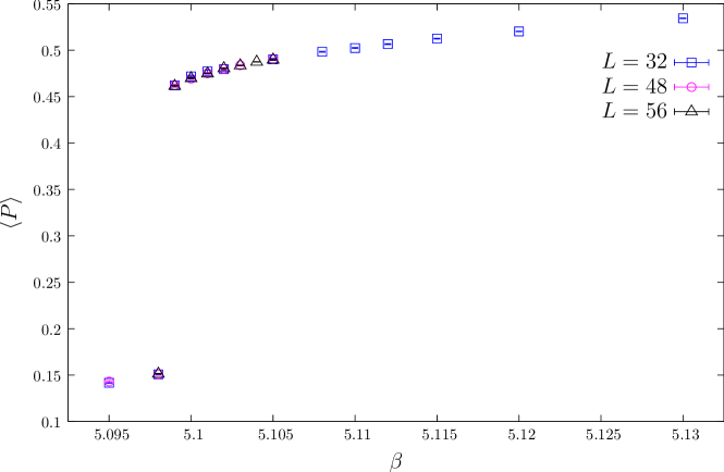
We begin by showing that a deconfining and chiral-symmetry-restoring first-order phase transition takes place at some critical $\beta_{c}$. In Fig. 1 we show the expectation value of the Polyakov loop $\langle P\rangle$, where $P(\vec{x})=\frac{1}{3}{\rm Re}\,{\rm tr}\,\tilde{P}(\vec{x})$, and $\tilde{P}(\vec{x})$ is the Polyakov line, i.e., the straight-line gauge transporter winding around the temporal direction at $\vec{x}$. A sudden jump is clearly visible between $\beta=5.098$ and $\beta=5.099$, indicating the presence of a first-order phase transition. The critical coupling for deconfinement, $\beta_{c}^{\rm dec}$, is therefore in the window $5.098<\beta_{c}^{\rm dec}<5.099$.

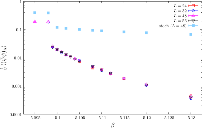
Next, in Fig. 2 we show the chiral condensate $\langle(\bar{\psi}\psi)_{\Lambda}\rangle$, defined as

$$\langle(\bar{\psi}\psi)_{\Lambda}\rangle=\int_{0}^{\Lambda}d\lambda\,\frac{2m}{\lambda^{2}+m^{2}}\,\rho(\lambda)\,.$$ (7)

We used $\Lambda=0.001$. It is evident that between $\beta=5.098$ and $\beta=5.099$ also this quantity jumps abruptly, decreasing by an order of magnitude. The critical coupling where the chiral transition takes place, $\beta_{c}^{\chi}$, is therefore in the same window $5.098<\beta_{c}^{\chi}<5.099$ as $\beta_{c}^{\rm dec}$. It is then very likely that $\beta_{c}^{\chi}=\beta_{c}^{\rm dec}$. Although the value we used for $\Lambda$ seems unreasonable as it is much smaller than the fermion mass, the effect that we are after, namely the presence of a first-order phase transition, should not depend on our choice for the cutoff. In fact, what we expect to cause the effect is a change in $\rho(0)$, i.e., in the density of the lowest modes. In Fig. 2 we also show the full chiral condensate (i.e., $\Lambda=\infty$) computed stochastically for one of the volumes. While the two quantities are numerically quite different, they nevertheless show the same critical behaviour, and so $\langle(\bar{\psi}\psi)_{\Lambda}\rangle$ can be reliably used to infer the presence of a phase transition.

Figure 3: Local spectral statistics $I_{s_{0}}$ as a function of $\lambda$ in the deconfined phase at $\beta=5.130$. Both numerical data and spline interpolations are shown. The values corresponding to Poisson and RMT are also shown. The value corresponding to the critical statistics, as determined in Ref. crit , is also shown together with its error band.

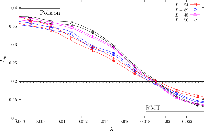
We now discuss the localisation properties of the eigenmodes. First of all, we show in Fig. 3 the typical behaviour of the spectral statistic $I_{s_{0}}$ as one moves along the spectrum in the deconfined phase. Here $\beta$ is fixed at $\beta=5.130$, and we scan the spectrum. Moving from the low end of the spectrum towards the bulk, a clear transition from Poisson to RMT statistics is observed. This shows that the lowest modes are localised, while higher up in the spectrum the eigenmodes are extended. Moreover, $I_{s_{0}}$ passes through the critical value where it is volume-independent (within errors), as it should be. This supports the expected universality of the critical statistics.

Figure 4: Mobility edge $\lambda_{c}$, determined as the point where $I_{s_{0}}(\lambda_{c})=I_{s_{0}}^{\rm crit}$, as a function of $\beta$. Quadratic fits to the data are also reported, for $L=48$ (long-dashed line) and $L=56$ (short-dashed line), with almost identical curves.

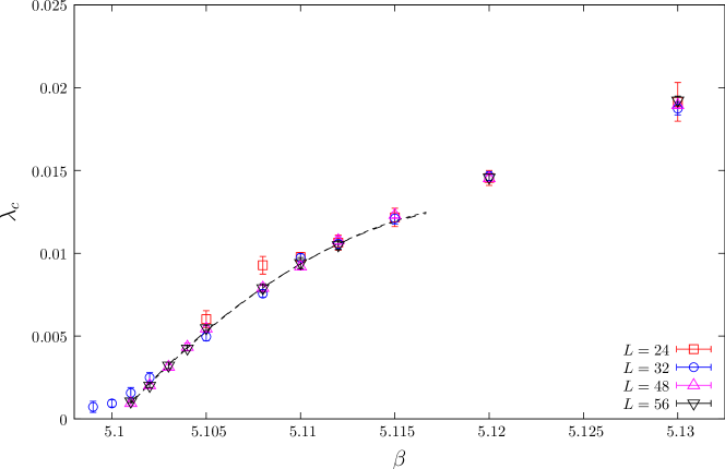
The volume-independence of $I_{s_{0}}$ where it crosses the critical value, $I_{s_{0}}^{\rm crit}$, shows that the latter can be used to reliably determine $\lambda_{c}$ via the relation $I_{s_{0}}(\lambda_{c})=I_{s_{0}}^{\rm crit}$, as discussed in section 2. Our results for $\lambda_{c}(\beta)$ determined in this way are shown in Fig. 4. Here the bin size for $\lambda$ is $w=0.001$. To find $\lambda_{c}$ we used a cubic spline interpolation $f(\lambda)$ of the numerical data. The error on the spline was determined as follows. For fixed $\{\lambda_{i}\}$, we generated 1000 synthetic sets of data points $\{I^{\rm synth}_{s_{0}}(\lambda_{i})\}$, following a Gaussian distribution centered at $I_{s_{0}}(\lambda_{i})$ and with standard deviation given by the corresponding error, and then computed the corresponding set of interpolating functions. The error $\delta f(\lambda)$ on the spline interpolation at a given $\lambda$ was then computed as the standard deviation of the set of such interpolating functions. We then determined the crossing points $\lambda_{\pm}$ by solving $f(\lambda_{\pm})\pm\delta f(\lambda_{\pm})=I_{s_{0}}^{\rm crit}$. The value of $\lambda_{c}$ was then determined as the average of $\lambda_{\pm}$, and the corresponding difference constitutes a first contribution to the uncertainty on $\lambda_{c}$. A second source of error is the uncertainty on the value of $I_{s_{0}}^{\rm crit}$, which has been determined numerically in Ref. crit . To take this into account, we repeated the determination of $\lambda_{\pm}$ using 1000 synthetic values of the critical $I_{s_{0}}$, generated according to a Gaussian distribution with mean equal to $I_{s_{0}}^{\rm crit}$ and standard deviation equal to the corresponding error. The final error on $\lambda_{c}$ was obtained by adding in quadrature the two sources of error. In Fig. 4 we also show fits to the data (with $L=48$ or $L=56$, and up to $\beta=5.112$) with a second-order polynomial, which yields for the critical point $\beta_{c}^{\rm loc}$ where localisation appears the value $\beta_{c}^{\rm loc}\simeq 5.1$. This value is quite close to $\beta_{c}^{\chi}$ and $\beta_{c}^{\rm dec}$. However, we cannot give a reliable estimate of the error on $\beta_{c}^{\rm loc}$, since it is difficult to control the systematic effects due to finite size on the determination of $\lambda_{c}$ in the vicinity of the transition, when this is very close to zero (see the discussion in section 2). Therefore, the method employed here does not allow us to determine $\beta_{c}^{\rm loc}$ with the same accuracy with which $\beta_{c}^{\chi}$ and $\beta_{c}^{\rm dec}$ can be obtained from the chiral condensate and the Polyakov loop, respectively.

Figure 5: Shape analysis for $N_{T}=4$ unimproved staggered fermions for several volumes and values of the gauge coupling (points), and for $N_{f}=2+1$ QCD at $\beta=3.75$, $N_{T}=4$ and $L=56$ (solid line; data taken from Ref. crit ). The points corresponding to Poisson and RMT statistics are also shown.

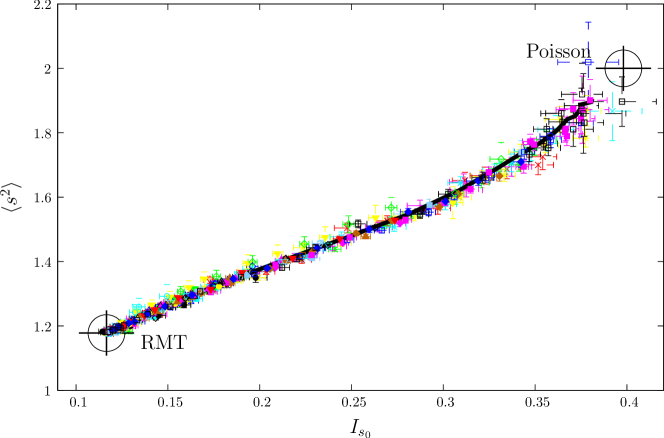
Before discussing other methods to determine $\beta_{c}^{\rm loc}$, it is worth comparing our results for the statistical properties of the spectrum with those obtained in QCD, in order to test whether there is a somewhat wider universality than just at the critical point $\lambda_{c}$ in the spectrum. As discussed in Ref. Giordano:2014qna , in QCD the unfolded level spacing distributions $P_{\lambda}(s)$ found in different parts of the spectrum lie on a universal path in the space of probability distributions, a path that is independent of volume, temperature and lattice spacing. This can be seen by plotting two different parameters of $P_{\lambda}(s)$ against each other (“shape analysis” shape_analysis ), thus taking a two-dimensional projection of this path, which should therefore yield a universal curve. In Fig. 5 we plot the second moment of the unfolded spacing distribution, $\langle s^{2}\rangle$, against $I_{s_{0}}$, with each data point corresponding to a specific point in the spectrum, and to a given system size and value of the gauge coupling. The data points indeed arrange themselves rather precisely on a single curve, which furthermore compares well with the one obtained in QCD Giordano:2014qna ; Nishigaki:2013uya .

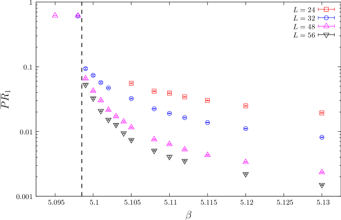
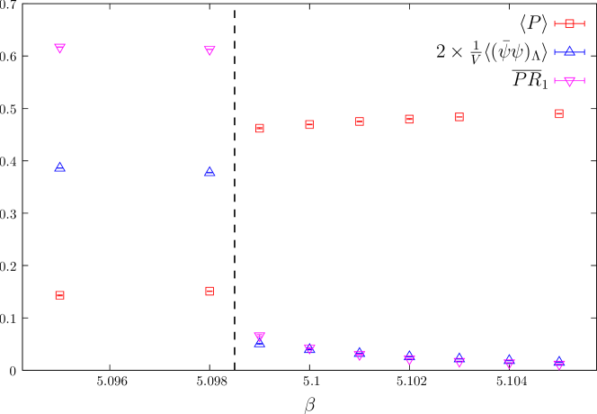
As we mentioned above and in the previous Section, the determination of $\lambda_{c}$ is difficult in the vicinity of the phase transition. For this reason, we have studied in detail the behaviour of the first eigenmode. In Fig. 6 we show the participation ratio $\overline{PR}_{1}=(N_{T}V)^{-1}\langle(IPR_{1})^{-1}\rangle$ of the first eigenmode averaged over configurations, as a function of $\beta$. This plot shows clearly that from $\beta=5.099$ up the first eigenmode is localised, with $\overline{PR}_{1}$ tending to zero as the volume is increased. This indicates that $5.098<\beta_{c}^{\rm loc}<5.099$, so that our results are compatible with $\beta_{c}^{\rm loc}=\beta_{c}^{\rm dec}=\beta_{c}^{\chi}$. For completeness, we thus show the Polyakov loop, the chiral condensate and the participation ratio of the first eigenmode together in Fig. 7.

Figure 6: Average participation ratio $\overline{PR}_{1}$ of the first eigenmode as a function of $\beta$. The dashed line at $\beta=5.0985$ is halfway through the region where the deconfining/chiral transition is expected to take place.

As a cross-check for the coincidence of $\beta_{c}^{\chi}$ and $\beta_{c}^{\rm loc}$, in Fig. 8 we show the quantity $\bar{\rho}_{0}$, defined as

$$\bar{\rho}_{0}\equiv\frac{1}{V\sqrt{\pi}\langle\lambda_{1}\rangle}\,.$$ (8)

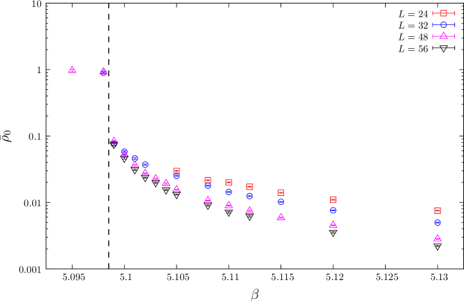
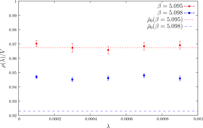
If the theory were quenched and only the topological sector $\nu=0$ contributed to the partition function, this would yield the spectral density at the origin, in case this were not vanishing. If the spectral density vanished at the origin like some power of $\lambda$, then this quantity would also vanish in the infinite-volume limit [see Eq. (5)]. We therefore expect this quantity to behave like $\rho(0)$ across the transition, namely to tend to a finite constant below $T_{c}$, and to zero above $T_{c}$, when the thermodynamic limit is taken. This expectation holds if the eigenvalues obey RMT and Poisson statistics, respectively, which in turn should be the case for delocalised and localised modes, respectively. In Fig. 8 one can clearly see a jump between $\beta=5.098$ and $\beta=5.099$, where $\bar{\rho}_{0}$ changes by an order of magnitude. Moreover, one can see that above $\beta=5.099$, $\bar{\rho}_{0}$ tends to zero as the volume increases. Despite it being above the jump, at $\beta=5.099$ one finds that $\bar{\rho}_{0}$ is constant within errors. Although the current statistical accuracy and the limited number of available volumes do not allow a definitive conclusion, this behaviour is most likely a finite-size effect. Indeed, as long as the volume is not larger than the typical size of the localised modes, these effectively look delocalised. In conclusion, even though we cannot assign this point to either phase with certainty, nevertheless the presence of a jump strongly suggests that it belongs to the localised phase. This conclusion would be consistent with the behaviour of $\overline{PR}_{1}$, shown in Fig. 6. In Fig. 9 we show that $\bar{\rho}_{0}$ compares indeed quite well with $\rho(\lambda\approx 0)$ in the chirally broken phase. The use of the quenched distribution Eq. (3) is justified by the fact that the first eigenvalue $\lambda_{1}$ is typically much smaller than the quark mass on our lattices.

Figure 7: Average Polyakov loop $\langle P\rangle$, chiral condensate $\langle(\bar{\psi}\psi)_{\Lambda}\rangle$ and average participation ratio $\overline{PR}_{1}$ of the first eigenmode, as a function of $\beta$. The coincidence of the jump in the three observables is evident.

4 Conclusions and outlook

In this paper we have studied the issue of localisation of the low Dirac eigenmodes in a toy model of QCD, consisting of unimproved staggered fermions interacting via SU$(3)$ gauge fields on a lattice of temporal extension $N_{T}=4$. While the low and high temperature phases of QCD are connected by an analytic crossover, such a model displays a genuine deconfining and (approximately) chirally-restoring first-order phase transition at some critical value of the gauge coupling $\beta$ unimproved0 ; unimproved1 ; unimproved . This allows us to study the relation between deconfinement, chiral restoration and localisation in a more clear-cut setting.

Our results indicate that the onset of localisation of the lowest Dirac eigenmodes takes place at the same critical coupling $\beta_{c}$ at which the system undergoes the first-order phase transition. While for $\beta<\beta_{c}$ all the modes are delocalised, for $\beta>\beta_{c}$ the lowest modes are localised up to a critical point $\lambda=\lambda_{c}(\beta)$ in the spectrum, which keeps increasing as $\beta$ is increased: this is fully analogous to what happens in QCD. In the light of the mechanism for localisation discussed in Ref. GKP2 , these results support our expectation that deconfinement triggers localisation of the lowest modes through the appearance, in the deconfined phase, of “islands” in the Polyakov line configuration, i.e., fluctuations of the Polyakov lines away from the ordered (trivial) value. The localised nature of these “islands” is also expected to play an important role in the depletion of the spectral region around the origin GKP2 , and therefore in the approximate restoration of chiral symmetry. Summarising, deconfinement appears to be the fundamental phenomenon triggering both chiral symmetry restoration and localisation of the low modes.

It would be interesting to study also other QCD-like models displaying a genuine phase transition. An obvious possibility is pure SU$(3)$ gauge theory. In contrast to that model, the one considered in the present paper possesses a true (albeit softly broken) chiral symmetry, and so the issue of chiral symmetry restoration is better defined. On the other hand, the presence of a first-order phase transition is here a lattice artifact that does not survive the continuum limit, while it does in pure-gauge SU$(3)$. For this reason, it would be worth studying the fate of localisation as one decreases the lattice spacing in the latter model.

Another interesting case would be the pure-gauge SU$(2)$ theory, where the deconfinement transition is second-order. A study of the near-critical behaviour of the lowest eigenmodes could then shed some light on how (if at all) the localisation transition depends on the order of the deconfinement transition.

Figure 8: Plot of $\bar{\rho}_{0}$, Eq. (8), as a function of $\beta$.

Figure 9: Comparison of the spectral density per unit volume with $\bar{\rho}_{0}=[V\sqrt{\pi}\langle\lambda_{1}\rangle]^{-1}$ in the chirally broken phase. Here $L=48$.

References

- (1) T. Banks and A. Casher, Nucl. Phys. B 169 (1980) 103.
- (2) Y. Aoki, Z. Fodor, S. D. Katz and K. K. Szabó, Jour. High Energy Phys. 01 (2006) 089 [hep-lat/0510084].
- (3) S. Borsányi, G. Endrődi, Z. Fodor, A. Jakovác, S. D. Katz, S. Krieg, C. Ratti and K. K. Szabó, Jour. High Energy Phys. 11 (2010) 077 [arXiv:1007.2580 [hep-lat]].
- (4) A. M. García-García and J. C. Osborn, Phys. Rev. D 75 (2007) 034503 [hep-lat/0611019].
- (5) T. G. Kovács and F. Pittler, Phys. Rev. Lett. 105 (2010) 192001 [arXiv:1006.1205 [hep-lat]].
- (6) F. Bruckmann, T. G. Kovács and S. Schierenberg, Phys. Rev. D 84 (2011) 034505 [arXiv:1105.5336 [hep-lat]].
- (7) T. G. Kovács and F. Pittler, Phys. Rev. D 86 (2012) 114515 [arXiv:1208.3475 [hep-lat]].
- (8) M. Giordano, T. G. Kovács and F. Pittler, PoS LATTICE 2013 (2013) 212 [arXiv:1311.1770 [hep-lat]].
- (9) M. Giordano, T. G. Kovács and F. Pittler, Phys. Rev. Lett. 112 (2014) 102002 [arXiv:1312.1179 [hep-lat]].
- (10) T. G. Kovács, Phys. Rev. Lett. 104 (2010) 031601 [arXiv:0906.5373 [hep-lat]].
- (11) G. Cossu and S. Hashimoto, Jour. High Energy Phys. 06 (2016) 056 [arXiv:1604.00768 [hep-lat]].
- (12) M. Giordano, T. G. Kovács and F. Pittler, Jour. High Energy Phys. 04 (2015) 112 [arXiv:1502.02532 [hep-lat]].
- (13) M. Giordano, T. G. Kovács and F. Pittler, Jour. High Energy Phys. 06 (2016) 007 [arXiv:1603.09548 [hep-lat]].
- (14) A. M. García-García and J. C. Osborn, Nucl. Phys. A 770 (2006) 141 [hep-lat/0512025].
- (15) E. V. Shuryak, Nucl. Phys. B 203 (1982) 93.
- (16) E. V. Shuryak, Nucl. Phys. B 203 (1982) 116.
- (17) E. V. Shuryak, Nucl. Phys. B 203 (1982) 140.
- (18) D. Diakonov and V. Y. Petrov, Phys. Lett. B 147 (1984) 351.
- (19) D. Diakonov and V. Y. Petrov, Nucl. Phys. B 272 (1986) 457.
- (20) D. Diakonov, Proc. Int. Sch. Phys. Fermi 130 (1996) 397 [hep-ph/9602375].
- (21) A. V. Smilga, Phys. Rev. D 46 (1992) 5598.
- (22) R. A. Janik, M. A. Nowak, G. Papp and I. Zahed, Phys. Rev. Lett. 81 (1998) 264 [hep-ph/9803289].
- (23) J. C. Osborn and J. J. M. Verbaarschot, Phys. Rev. Lett. 81 (1998) 268 [hep-ph/9807490].
- (24) J. C. Osborn and J. J. M. Verbaarschot, Nucl. Phys. B 525 (1998) 738 [hep-ph/9803419].
- (25) A. M. García-García and J. C. Osborn, Phys. Rev. Lett. 93 (2004) 132002 [hep-th/0312146].
- (26) D. Diakonov, Nucl. Phys. Proc. Suppl. 195 (2009) 5 [arXiv:0906.2456 [hep-ph]].
- (27) F. Bruckmann, D. Nógrádi and P. van Baal, Acta Phys. Polon. B 34 (2003) 5717 [hep-th/0309008].
- (28) E. Shuryak and T. Sulejmanpasic, Phys. Rev. D 86 (2012) 036001 [arXiv:1201.5624 [hep-ph]].
- (29) E. Poppitz, T. Schäfer and M. Ünsal, JHEP 1303 (2013) 087 [arXiv:1212.1238 [hep-th]].
- (30) F. Karsch, E. Laermann and C. Schmidt, Phys. Lett. B 520 (2001) 41 [hep-lat/0107020].
- (31) P. de Forcrand and O. Philipsen, Nucl. Phys. B 673 (2003) 170 [hep-lat/0307020].
- (32) P. de Forcrand and O. Philipsen, Jour. High Energy Phys. 11 (2008) 012 [arXiv:0808.1096 [hep-lat]].
- (33) M. Giordano, T. G. Kovács, S. D. Katz and F. Pittler, PoS LATTICE 2014 (2014) 214 [arXiv:1410.8392 [hep-lat]].
- (34) M. Giordano, T. G. Kovács and F. Pittler, Int. J. Mod. Phys. A 29 (2014) 1445005. [arXiv:1409.5210 [hep-lat]].
- (35) J. J. M. Verbaarschot and T. Wettig, Ann. Rev. Nucl. Part. Sci. 50 (2000) 343 [hep-ph/0003017].
- (36) P. de Forcrand, AIP Conf. Proc. 892 (2007) 29 [hep-lat/0611034].
- (37) A. Tomiya, G. Cossu, S. Aoki, H. Fukaya, S. Hashimoto, T. Kaneko and J. Noaki, arXiv:1612.01908 [hep-lat].
- (38) P. W. Anderson, Phys. Rev. 109 (1958) 1492.
- (39) P. A. Lee and T. V. Ramakrishnan, Rev. Mod. Phys. 57 (1985) 287.
- (40) F. Evers and A. D. Mirlin, Rev. Mod. Phys. 80 (2008) 1355 [arXiv:0707.4378 [cond-mat.mes-hall]].
- (41) K. Slevin and T. Ohtsuki, Phys. Rev. Lett. 78 (1997) 4083 [cond-mat/9704192 [cond-mat.dis-nn]].
- (42) M. Mehta, Random Matrices (Academic Press, San Diego, 1991).
- (43) L. Ujfalusi, M. Giordano, F. Pittler, T. G. Kovács and I. Varga, Phys. Rev. D 92 (2015) 094513 [arXiv:1507.02162 [cond-mat.dis-nn]].
- (44) L. Ujfalusi and I. Varga, Phys. Rev. B 91 (2015) 184206 [arXiv:1501.02147 [cond-mat.dis-nn]].
- (45) B. I. Shklovskii, B. Shapiro, B. R. Sears, P. Lambrianides and H. B. Shore, Phys. Rev. B 47 (1993) 11487.
- (46) E. Hofstetter and M. Schreiber, Phys. Rev. B 49 (1994) 14726.
- (47) P. J. Forrester, Nucl. Phys. B 402 (1993) 709.
- (48) S. M. Nishigaki, P. H. Damgaard and T. Wettig, Phys. Rev. D 58 (1998) 087704 [hep-th/9803007].
- (49) S. M. Nishigaki, PoS LATTICE 2015 (2016) 057 [arXiv:1606.00276 [hep-lat]].
- (50) I. Varga, E. Hofstetter, M. Schreiber and J. Pipek, Phys. Rev. B 52 (1995) 7783.
- (51) S. M. Nishigaki, M. Giordano, T. G. Kovács and F. Pittler, PoS LATTICE 2013 (2014) 018 [arXiv:1312.3286 [hep-lat]].