Total variation denoising in $l^{1}$ anisotropy

Abstract

We aim at constructing solutions to the minimizing problem for the variant of Rudin-Osher-Fatemi denoising model with rectilinear anisotropy and to the gradient flow of its underlying anisotropic total variation functional. We consider a naturally defined class of functions piecewise constant on rectangles ($PCR$). This class forms a strictly dense subset of the space of functions of bounded variation with an anisotropic norm. The main result shows that if the given noisy image is a $PCR$ function, then solutions to both considered problems also have this property. For $PCR$ data the problem of finding the solution is reduced to a finite algorithm. We discuss some implications of this result, for instance we use it to prove that continuity is preserved by both considered problems.

MSC: 68U10, 35K67, 35C05, 49N60, 35B65

Keywords: denoising, Rudin-Osher-Fatemi model, total variation flow, anisotropy, rectangles, rectilinear polygons, piecewise constant solutions, regularity, tetris

1 Introduction

In [20], the authors introduced the anisotropic version of the celebrated model by Rudin, Osher and Fatemi (ROF) [31] of total variation based noise removal from a corrupted image. The idea was to substitute the total variation term in the energy functional

$$\int_{\Omega}|Du|+\frac{1}{2\lambda}\int_{\Omega}(u_{0}-u)^{2}\,\mathrm{d}\mathcal{L}^{2},$$ (1)

by an anisotropic total variation term suitably chosen for a particular given image:

$$\int_{\Omega}|Du|_{\varphi}+\frac{1}{2\lambda}\int_{\Omega}(u_{0}-u)^{2}\,\mathrm{d}\mathcal{L}^{2}.$$ (2)

Although from the point of view of image processing it is most natural to consider the domain $\Omega$ being a rectangle, in principle it can be any open bounded set with reasonably regular (e. g. Lipschitz) boundary, or the whole plane $\mathbb{R}^{2}$. The function $|\cdot|_{\varphi}\colon\mathbb{R}^{2}\to[0,+\infty[$ encoding the anisotropy is assumed to be convex, positively 1-homogeneous and such that $|\boldsymbol{x}|_{\varphi}>0$ if $\boldsymbol{x}\neq 0$. Observe that (2) is a generalization of (1) for which $|\cdot|_{\varphi}$ is the Euclidean norm, $|\cdot|$. In this case, the associated Wulff shape,

$$W_{\varphi}:=\{\boldsymbol{y}\in\mathbb{R}^{2}\colon\boldsymbol{y}\cdot\boldsymbol{x}\leq|\boldsymbol{x}|_{\varphi}\text{ for all }\boldsymbol{x}\in\mathbb{R}^{2}\},$$

is exactly the unit ball with respect to the Euclidean distance. Because of that, minimizers of (1) give rise to convex shapes which are smooth (as is the Euclidean ball). If, instead, $|\cdot|_{\varphi}$ is a crystalline anisotropy (in the sense that the Wulff shape is a polygon), then minimizers of (2) give rise to convex shapes which are compatible with the Wulff shape, and therefore not smooth anymore.

This new approach has been successfully applied to most of the classical problems in image processing including denoising (see [32],[23] and [24]), cartoon extraction [8], inpainting [17], deblurring [18] or denoising and deblurring of 2-D bar codes [19]. In most of these works, the chosen anisotropy is the $l^{1}$ norm in the plane; i. e. $|\boldsymbol{x}|_{\varphi}=|\boldsymbol{x}|_{1}:=|x_{1}|+|x_{2}|$. In this case, the corresponding Wulff shape is the unit ball with respect to the $l^{\infty}$ distance; i. e. a square.

In the present paper, we focus on the case $|\boldsymbol{x}|_{\varphi}=|\boldsymbol{x}|_{1}$. We give an explicit expression for the minimizer when the corrupted image $u_{0}$ belongs to the class of functions piecewise constant on rectangles (as in the case of applications), denoted by $PCR(\Omega)$ (see section 2.3 for precise definitions). The minimizer turns out to belong to $PCR(\Omega)$.

Let us briefly explain the algorithm for construction of the minimizer. Given a function $u_{0}\in PCR(\Omega)$, we consider $G_{u_{0}}$, the minimal grid associated to the level sets of $u_{0}$ (which are rectilinear polygons, precise definitions are given in section 2.3). Then, we construct level sets $F_{k}$ of $u$, starting with highest values of $u$, as follows:

• Step $1$. Take as $F_{1}$ the largest minimizer of the following Cheeger quotient $\mathcal{J}_{1}$ among all possible rectilinear polygons $E$ contained in $\overline{\Omega}$ subordinate to $G_{u_{0}}$:

  $$\mathcal{J}_{1}(E)=\frac{\mathcal{H}^{1}(\partial E\cap\Omega)-\frac{1}{\lambda}\int_{E}u_{0}\,\,\mathrm{d}\mathcal{L}^{2}}{\mathcal{L}^{2}(E)}.$$

• Step $k$. Denote $\check{F}_{k}=\bigcup_{i=1}^{k-1}F_{i}$. If $\overline{\Omega}=\check{F}_{k}$, stop. Otherwise, denote by $F_{k}$ the largest minimizer of the following Cheeger quotient $\mathcal{J}_{k}$ among all possible rectilinear polygons contained in $\overline{\Omega\setminus\check{F}_{k}}$ subordinate to $G_{u_{0}}$:

  $$\mathcal{J}_{k}(E)=\frac{\mathcal{H}^{1}(\partial E\cap\Omega\setminus\check{F}_{k})-\mathcal{H}^{1}(\partial E\cap\partial\check{F}_{k})-\frac{1}{\lambda}\int_{E}u_{0}\,\,\mathrm{d}\mathcal{L}^{2}}{\mathcal{L}^{2}(E)}.$$

In each rectilinear polygon $F_{k}$ of resulting decomposition of $\Omega$, we define

$$u|_{F_{k}}=-\lambda\mathcal{J}_{k}(F_{k}).$$ (3)

In order to prove that $u$ given by this algorithm is in fact the minimizer, we perform a rather involved mathematical analysis starting from the following observation (the Euler-Lagrange equation for (2)): $u$ is a minimizer of (2) if and only if $\frac{u-u_{0}}{\lambda}$ belongs to negative subdifferential of the energy functional $TV_{\varphi,\Omega}$ on $L^{2}(\Omega)$ defined by

$$TV_{\varphi,\Omega}(u)=\left\{\begin{array}[]{ll}\int_{\Omega}|Du|_{\varphi}&\text{ if }u\in BV(\Omega),\\ +\infty&\text{ otherwise.}\\ \end{array}\right.$$

This anisotropic energy functional was studied in [28] in cases that $\Omega=\mathbb{R}^{N}$ or $\Omega$ is a bounded, open, smooth subset of $\mathbb{R}^{N}$, coupled with Dirichlet boundary conditions. The author characterized the subdifferential as the set of elements of form $\mathrm{div}\,\boldsymbol{\xi}$ with $\boldsymbol{\xi}$ satisfying certain conditions (see Theorem 1). In the case that $\Omega$ is a rectilinear polygon and $u_{0}\in PCR(\Omega)$, the condition that the solution $u$ to

$$\min_{u\in BV(\Omega)}TV_{1,\Omega}(u)+\frac{1}{2\lambda}\int_{\Omega}(u-u_{0})^{2}\,\mathrm{d}\mathcal{L}^{2}$$ (4)

also belongs to $PCR(\Omega)$ follows from finding a vector field $\boldsymbol{\xi}\in L^{\infty}(\Omega)$ such that $|\boldsymbol{\xi}|_{\infty}\leq 1$ $\mathcal{L}^{2}$-a. e., a suitable compatibility condition on the jump set of $u$ is satisfied (Lemma 1) and $\mathrm{div}\,\boldsymbol{\xi}$ is piecewise constant on rectangles. Note that once we know that there are such $u$ and $\boldsymbol{\xi}$, and rectilinear polygons $F_{k}$ are ordered level sets of $u$, (3) follows by averaging $u=u_{0}+\lambda\mathrm{div}\,\boldsymbol{\xi}$ over each $F_{k}$.

We construct the vector field $\boldsymbol{\xi}$ together with $u$ in Theorem 5 by minimizing the $L^{2}$ norm of the divergence over vector fields satisfying compatibility conditions. Then, in order to show that the divergence is piecewise constant on rectangles, we rely on an auxiliary result (Theorem 3) in which we prove that a certain anisotropic Cheeger-type functional on sets (related to the algorithm sketched above) is indeed minimized by a rectilinear polygon. In the proof of that result, an important point is that, due to the structure of the Cheeger quotient, we construct approximate minimizers that belong to a finite class of rectilinear polygons subordinate to $G_{u_{0}}$. As the set of characteristic functions of rectilinear polygons is not compact with respect to $TV_{1,\Omega}$, this finiteness is essential.

On the other hand, our analysis shows that any function piecewise constant on rectangles belongs to domain of the subdifferential of $TV_{1,\Omega}$ (Lemma 1), and that this class of functions is preserved by the gradient descent flow of this functional,

$$\left\{\begin{array}[]{l}u_{t}\in-\partial TV_{1,\Omega},\\ u|_{t=0}=u_{0}.\end{array}\right.$$ (5)

In principle, one could try to deduce this result from Theorem 5 by analyzing the discretization of (5) with respect to time variable (which coincides with a sequence of problems of form (4) with $\lambda=\Delta t$). Instead, in Theorems 6 and 7 we do this directly, constructing the vector field that encodes the solution by means of a number of variational problems. This way we obtain a finite explicit algorithm for obtaining $u$, with a different structure than that in Theorem 5. In particular, we use the semigroup property of solutions to (5). The results in this case say that in any of a finite number of intervals between two subsequent time instances of merging, $u_{t}$ is a fixed function in $PCR(\Omega)$. The exact form of $u_{t}$ is (again) determined by solving a number of (different) Cheeger-type problems. In this case, the algorithm is slightly more complicated. Given a function $w\in PCR(\Omega)$, we consider again $G_{w}$ as the minimal grid associated to the level sets of $w$. For each level set $Q$, we label each part of the boundary as positive, and we say that it belongs to $\partial Q^{+}$ (resp. negative, $\partial Q^{-}$), if the value of $u(t,\cdot)$ inside $Q$ is higher than (resp. lower than) the value of the level set adjacent to this part of the boundary (thus, we define a consistent signature, see subsection 2.3). Then, we produce a decomposition of each level set into a family of rectilinear polygons and related consisted signature by means of an algorithm similar to the one for the minimizer. Finally, to each rectilinear polygon in the decomposition, a constant related to the signature is assigned. It is proved that $u_{t}$ coincides with this exact constant (up to next merging time, when the algorithm has to be reinitialized).

We stress that the problem of determining evolution is nontrivial, as at time instances of merging, breaking may occur along certain line segments, leading to expansion of jump set of the solution.

As $\partial TV_{1,\Omega}$ is a monotone operator, for any datum $u_{0}\in L^{2}(\Omega)$ and a sequence $u_{0,n}\in L^{2}(\Omega)$, $n=1,2,\ldots$ such that $u_{0,n}\to u_{0}$ in $L^{2}(\Omega)$, solutions $u_{n}$ with datum $u_{0,n}$ converge to the solution with datum $u_{0}$. It is easy to check that $PCR(\Omega)$ is dense in $L^{2}(\Omega)$. In fact, $PCR(\Omega)$ is even strictly dense in $BV(\Omega)$ (in the sense of seminorm $\int_{\Omega}|\nabla u|_{1})$, see [12, Theorem 3.4]. Therefore, we do not only give the explicit solution when initial datum belongs to $PCR(\Omega)$, but we provide an algorithm to compute the solution for any initial corrupted image with the most natural approximation to it (with functions belonging to the domain of the subdifferential).

The idea of a finite dimensional approximation of problem (4) based on $PCR$ functions is already present in literature. For instance, in [21], the authors prove that the solutions to (4) where the functional is replaced with its restrictions (discretizations) to functions piecewise constant on finer and finer grids (and datum $u_{0}$ replaced by its suitable projections) converge to the solution to (4). Our result implies that minimizers to those discrete problems are themselves actual solutions to (4) (with projected datum).

For a typical example, the space of $PCR$ functions associated with the $(M+1)\times(N+1)$ Cartesian grid in a rectangle $\Omega=[0,M]\times[0,N]$ is isomorphic to $\mathbb{R}^{M\times N}=(u_{i,j};\;i=1,\ldots,M;\;j=1,\ldots,N)$. Our result shows that the functional $TV_{1,\Omega}$ restricted to this subspace of $PCR(\Omega)$ is equivalent to the discrete Ising-type functional

$$\sum\{|u_{i,j}-u_{k,l}|\colon i,k=1,\ldots,M;\;j,l=1,\ldots,N;\;|i-k|+|j-m|=1\}.$$ (6)

This information means that one can use one of many efficient algorithms, such as graph-cut based algorithms (see e. g. [16, 25] and references therein) devised for minimizing discrete functionals involving terms of type (6) to obtain the exact (up to machine error) solution to (4). We note here that the algorithm proposed by us is of theoretical significance as a tool allowing us to prove Theorem 5.

Our approach allows us to prove some continuity results about solutions to (4) and (5). In particular, if $\Omega$ is a rectangle or the plane, we prove that if the datum $u_{0}$ admits a modulus of continuity of a certain form, then solutions do as well (Theorems 8 and 9). Analogous results were obtained in the isotropic case in [14, 15]. The method there involves considering distance between level sets of solution. First, the authors show that the jump set of solution is contained (up to a $\mathcal{H}^{1}$-negligible set) in the jump set of initial datum. We point out that such a result is not true in our case since breaking may appear (see Example 1). Very recently, the continuity result for minimizers of (2) in convex domains has been proved to hold in the case of general anisotropies with different methods [27]. We still choose to include continuity results in this paper, mainly because the technique used here is very much different. The results are basically corollaries of Lemmata 5 and 6, which assert non-increasing of maximal jump on any length scale for $PCR$ data. The Lemmata are of independent interest from the point of view of computations, as discrete versions of continuity estimates. Example 3 shows that continuity is not preserved in general, either by (4) or (5), if $\Omega$ is not convex.

At this point we note that our results can be seen as generalization of observations concerning 1-D problems with total variation. Indeed, in 1-D it is easy to see that piecewise constant data are preserved (and consequently, that continuity is preserved), in fact much more is true, as in that case $|\nabla u|\leq|\nabla u_{0}|$ as measures [10, Corollary 3.2]. The particular simplicity of 1-D case allows for very detailed description of solutions (see e. g. [9, 26, 30]).

Finally, we remark that our description of solutions shares a connection on the formal level to ideas in [11] (see also other papers referenced there). In [11], the authors show that solutions to gradient flow equations of typical discretizations of linear growth functionals are piecewise linear in time, and give an explicit expression involving suitably defined nonlinear spectral decomposition. Having obtained finite reduction of (5) in Theorem 7, we can use it to recover spectral decomposition of $u_{0}\in PCR(\Omega)$ with respect to (5) via [11, Conclusion 2 and Theorem 4.13].

The plan of the paper is as follows. In section 2, we give some notation and preliminaries on rectilinear geometry, $BV$ functions, $L^{2}$-divergence vector fields as well as the anisotropic total variation and its gradient descent flow in $L^{2}$. In section 3, we study an auxiliary Cheeger-type problem in rectilinear geometry. Next, in sections 4 and 5 we give explicit solutions to (4) and (5) in the case that $u_{0}\in PCR(\Omega)$, where $\Omega$ is a rectilinear polygon. In section 6, we transfer the results to the case $\Omega={\mathbb{R}^{2}}$. The idealized setting of the whole plane ${\mathbb{R}^{2}}$ is convenient for discussing examples (from the point of view of images, it corresponds to a discrete feature set against a uniform background). Since the construction of solutions is similar to the previous cases, we only point out the main differences and state the results. Section 7 is devoted to the study of preservation of moduli of continuity. Finally, in section 8, we show the power of our approach by explicitly computing the solutions for some data, including the effects of bending and creation of singularities. After that we end up with some conclusions.

2 Notation and preliminaries

2.1 Balls

By $B_{\varphi}(\boldsymbol{x},r)$ we denote the ball in $\mathbb{R}^{N}$ with respect to norm $|\cdot|_{\varphi}$, centered at $\boldsymbol{x}$, of radius $r$. For the ball with respect to the Euclidean norm, we write simply $B(\boldsymbol{x},r)$. Symbols $B_{\varphi}(r),B(r)$ stand for balls centered at the origin.

2.2 Measures. Lebesgue and Bochner spaces

We denote by $\mathcal{L}^{N}$ and $\mathcal{H}^{N-1}$ the $N$-dimensional Lebesgue measure and the $(N-1)$-dimensional Hausdorff measure in $\mathbb{R}^{N}$, respectively. If $A\subset\mathbb{R}^{N}$ is a set of positive (possibly inifinite) $\mathcal{L}^{N}$ measure, we denote by $L^{p}(A)$, $1\leq p\leq\infty$ the Lebesgue space of functions integrable with power $p$ with respect to $\mathcal{L}^{N}$. On the other hand, if $A\subset\mathbb{R}^{N}$ has finite $\mathcal{H}^{N-1}$ measure (e. g. $A$ is the boundary of a Lipschitz domain), $L^{p}(A)$ denotes the Lebesgue space of functions integrable with power $p$ with respect to $\mathcal{H}^{N-1}$. We adopt similar notation for spaces $L^{p}(A,\mathbb{R}^{k})$, $k=2,3,\ldots$ Whenever it is clear, we adopt the convention that an equality or inequality between two measurable functions holds in the sense of Lebesgue spaces, i. e. almost everywhere with respect to the corresponding (implicitly specified) measure, unless otherwise stated.

If $]T_{1},T_{2}[\subset\mathbb{R}$ and $X$ is a Banach space, we denote by $L^{p}(]T_{1},T_{2}[,X)$ the usual space of Bochner measurable functions $f\colon]T_{1},T_{2}[\to X$ s. t. $\int_{T_{1}}^{T_{2}}\|f\|_{X}^{p}<\infty$. By $L_{w}^{p}(]T_{1},T_{2}[,X)$ we denote the analogous space of weakly measurable functions (see [4, Chapter I]).

2.3 Rectilinear polygons

We denote by $\mathcal{R}$ the set of closed rectangles in the plane whose sides are parallel to the coordinate axes, and by $\mathcal{I}$, the set of all horizontal and vertical closed line segments of finite length in the plane.

Figure 1: An example of a rectilinear polygon $F$ and a grid $G$. There holds $G=G(F)$ and $F\in\mathcal{F}(G)$.

We call $F\subset\mathbb{R}^{2}$ a rectilinear polygon if $F=\bigcup\mathcal{R}_{F}$ with a finite $\mathcal{R}_{F}\subset\mathcal{R}$. We denote by $\mathcal{F}$ the family of all rectilinear polygons. Similarly, we call $C\subset{\mathbb{R}^{2}}$ a rectilinear curve if $C=\bigcup\mathcal{I}_{C}$ with a finite $\mathcal{I}_{C}\subset\mathcal{I}$. We denote by $\mathcal{C}$ the set of all recilinear curves.

We call any finite set $G$ of horizontal and vertical lines in the plane a grid. If $F$ is a rectilinear polygon, we denote by $G(F)$ the minimal grid such that each side of $F$ is contained in a line belonging to $G(F)$. If $C$ is a rectilinear curve, we denote by $G(C)$ the minimal grid with the property that there exists $\mathcal{I}_{C}\subset\mathcal{I}$, $C=\bigcup\mathcal{I}_{C}$ such that all endpoints of intervals in $\mathcal{I}_{C}$ are vertices of $G(C)$.

Given a grid $G$, we denote

• by $\mathcal{I}(G)$ the set of line segments connecting adjacent vertices of $G$,

• by $\mathcal{R}(G)$ the set of rectangles whose sides belong to $\mathcal{I}(G)$,

• by $\mathcal{F}(G)$ the set of rectilinear polygons of form $\bigcup\mathcal{R}_{F}$ with a finite non-empty $\mathcal{R}_{F}\subset\mathcal{R}(G)$.

Note that all of the above are finite sets.

It is also convenient to introduce the following notions of partitions of rectilinear polygons and signatures for their boundaries. Let $\Omega$ be a rectilinear polygon. We say that a finite family $\mathcal{Q}$ of rectilinear polygons with disjoint interiors is a partition of $\Omega$ if $\Omega=\bigcup\mathcal{Q}$. If $G$ is a grid, we say that a partition $\mathcal{Q}$ of $\Omega$ is subordinate to $G$ if $\mathcal{Q}\subset\mathcal{F}(G)$. Let $F$ be a rectilinear polygon and let $G$ be a grid. We say that $(\partial F^{+},\partial F^{-})\in\mathcal{C}\times\mathcal{C}$ is a signature for $\partial F$ (or for $F$) if $\partial F^{\pm}\subset\partial F$ and $\mathcal{H}^{1}(\partial F^{+}\cap\partial F^{-})=0$. We say that a signature $(\partial F^{+},\partial F^{-})$ for $\partial F$ is subordinate to $G$ if both $\partial F^{\pm}$ are subordinate to $G$. We say that

$$\mathcal{S}\colon\mathcal{Q}\ni Q\mapsto\mathcal{S}(Q)=(\partial Q^{+},\partial Q^{-})\in\mathcal{C}\times\mathcal{C}$$

is a consistent signature for $\mathcal{Q}$ if

• for each $Q\in\mathcal{Q}$, $\mathcal{S}(Q)=(\partial Q^{+},\partial Q^{-})$ is a signature for $\partial Q$ and

• for each pair $Q,Q^{\prime}\in\mathcal{Q}$, if $\boldsymbol{x}\in\partial Q^{\pm}\cap Q^{\prime}$ then $\boldsymbol{x}\in\partial Q^{\prime\mp}$.

We say that a consistent signature $\mathcal{S}$ for $\mathcal{Q}$ is subordinate to $G$ if for each $Q\in\mathcal{Q}$, $\mathcal{S}(Q)$ is subordinate to $G$.

(a) A consistent singature $\mathcal{S}\colon Q_{i}\mapsto(\partial Q_{i}^{+},\partial Q_{i}^{-})$ for $\mathcal{Q}=\{Q_{1},Q_{2},Q_{3}\}$. Dashed lines denote $\partial Q_{i}^{+}$, dotted lines denote $\partial Q_{i}^{-}$, $i=1,2,3$.

(b) The graph of a function $w\in PCR([0,2]^{2})$ such that $\mathcal{S}=\mathcal{S}_{w}$.

(c) Not a consistent signature.

Figure 2: Examples of signatures.

Now, we give a precise definition of the class of functions piecewise constant on rectangles that we will work with. Let $\Omega$ be a rectangle and let $w\in L^{1}(\Omega)$. We write $w\in PCR(\Omega)$ if $w$ has a finite number of level sets of positive $\mathcal{L}^{2}$ measure, and each one is a rectilinear polygon up to a $\mathcal{L}^{2}$-null set. We denote the family of level sets of a function $w\in PCR(\Omega)$ by $\mathcal{Q}_{w}$. $\mathcal{Q}_{w}$ is a partition of $\Omega$ in the sense of the definition in the previous paragraph.

Furthermore, we put $G_{w}=\bigcup_{Q\in\mathcal{Q}_{w}}G(Q)$, $\mathcal{I}_{w}=\mathcal{I}(G_{w})$, $\mathcal{R}_{w}=\mathcal{R}(G_{w})$, $\mathcal{F}_{w}=\mathcal{F}(G_{w})$. Again, these are all finite sets.

Given $w\in PCR(\Omega)$ we define the signature induced by $w$, $\mathcal{S}_{w}\colon\mathcal{Q}_{w}\ni Q\mapsto(\partial Q^{+},\partial Q^{-})$, setting

$$\partial Q^{+}=\{\boldsymbol{x}\in\partial Q\colon\boldsymbol{x}\in Q^{\prime}\in\mathcal{Q}_{w},w|_{Q^{\prime}}<w|_{Q}\}$$

$$\partial Q^{-}=\{\boldsymbol{x}\in\partial Q\colon\boldsymbol{x}\in Q^{\prime}\in\mathcal{Q}_{w},w|_{Q^{\prime}}>w|_{Q}\},$$

for each $Q\in\mathcal{Q}_{w}$. Here and in many other places we abuse notation slightly, identifying the constant function $w|_{Q}$ with its value. The signature induced by $w$ is a consistent signature for $\mathcal{Q}_{w}$ subordinate to $G_{w}$.

2.4 Functions of bounded variation and sets of finite perimeter

We use standard notation and concepts related to $BV$ functions as in [2]; in particular, given $u\in BV(\Omega)$, we write $\nabla u\mathcal{L}^{N}$ and $D^{s}u$ for the absolutely continuous and singular part of $Du$ with respect to the Lebesgue measure $\mathcal{L}^{N}$, $u^{\pm}(x)$ for the lower and upper approximate limits of $u$ at $x\in\Omega$ and $J_{u}$ for its jump set, i. e. the set of points where $u^{+}\neq u^{-}$. Finally, $\frac{Du}{|Du|}$ denotes the Radon-Nikodym derivative of $Du$ with respect to its total variation $|Du|$.

The family $PCR(\Omega)$ introduced in the previous subsection is a linear subspace of $BV(\Omega)$. If $w\in PCR(\Omega)$, we have

$$J_{w}=\bigcup_{Q\in\mathcal{Q}_{w}}\partial Q^{+}=\bigcup_{Q\in\mathcal{Q}_{w}}\partial Q^{-},\qquad w^{\pm}|_{\partial Q^{\pm}}=w|_{Q}\,,$$

where $Q\mapsto(\partial Q^{+},\partial Q^{-})$ is the signature induced by $w$. Furthermore, we have

$$|Dw|=(w^{+}-w^{-})\mathcal{H}^{1}\!\!\mathop{\hbox{ \vrule height=7.0pt,width=0.5pt,depth=0.0pt\vrule height=0.5pt,width=6.0pt,depth=0.0pt}}\nolimits J_{w}=\bigcup_{Q\in\mathcal{Q}_{w}}w|_{Q}(\mathcal{H}^{1}\!\!\mathop{\hbox{ \vrule height=7.0pt,width=0.5pt,depth=0.0pt\vrule height=0.5pt,width=6.0pt,depth=0.0pt}}\nolimits\partial Q^{+}-\mathcal{H}^{1}\!\!\mathop{\hbox{ \vrule height=7.0pt,width=0.5pt,depth=0.0pt\vrule height=0.5pt,width=6.0pt,depth=0.0pt}}\nolimits\partial Q^{-}).$$ (7)

Given an open set $\Omega\subseteq\mathbb{R}^{N}$ and a Lebesgue measurable subset $E$ of $\mathbb{R}^{N}$, we say that $E$ has finite perimeter in $\Omega$ if $\chi_{E}\in BV(\Omega)$ and we write ${\rm Per}(E,\Omega):=|D\chi_{E}|(\Omega)$. If $E$ has finite perimeter in $\mathbb{R}^{N}$, we write ${\rm Per}(E):={\rm Per}(E,\mathbb{R}^{N})$.

If $E$ is a set of finite perimeter in $\mathbb{R}^{N}$, the jump set of $\chi_{E}$ is $\mathcal{H}^{N-1}$-equivalent to the reduced boundary $\partial^{*}E$ defined by the following. We say a point $\boldsymbol{x}\in\mathbb{R}^{N}$ belongs to $\partial^{*}E$ if $|D\chi_{E}|(B(\boldsymbol{x},\varrho))>0$ for all $\varrho>0$ and quantity $\frac{D\chi_{E}(B(\boldsymbol{x},\varrho))}{|D\chi_{E}|(B(\boldsymbol{x},\varrho))}$ has a limit that belongs to $\mathbb{S}^{N-1}$ as $\varrho\to 0^{+}$. If these conditions hold, we denote this limit by $\boldsymbol{\nu}^{E}(\boldsymbol{x})$. There holds

$$\partial^{*}E\subset\partial^{\frac{1}{2}}E=\left\{\boldsymbol{x}\in\mathbb{R}^{N}:\lim_{\varrho\to 0^{+}}\frac{\mathcal{L}^{N}(B(\boldsymbol{x},\varrho)\cap E)}{\mathcal{L}^{N}(B(\boldsymbol{x},\varrho))}=\frac{1}{2}\right\},$$

also $\mathcal{H}^{N-1}\left(\partial^{\frac{1}{2}}E\setminus\partial^{*}E\right)=0$ and $\mathcal{H}^{N-1}$-almost every point in $\mathbb{R}^{N}$ is either a Lebesgue point for $\chi_{E}$ or belongs to $\partial^{*}E$.

2.5 Traces of $L^{2}$-divergence vector fields

We consider the space

$$X_{\Omega}=\left\{\boldsymbol{z}\in L^{\infty}(\Omega,\mathbb{R}^{N})\,:\ \,\mathrm{div}\,\boldsymbol{z}\in L^{2}(\Omega)\right\}\,.$$ (8)

In [3, Theorem 1.2], the weak trace on the boundary of a bounded Lipschitz domain $\Omega$ of the normal component of $\boldsymbol{z}\in X_{\Omega}$ is defined. Namely, it is proved that the formula

$$\left\langle[\boldsymbol{z},\boldsymbol{\nu}^{\Omega}]\,,\,\rho\right\rangle:=\int_{\Omega}\rho\,\mathrm{div}\,\boldsymbol{z}\,\mathrm{d}\mathcal{L}^{N}+\int_{\Omega}\boldsymbol{z}\cdot\nabla\rho\,\mathrm{d}\mathcal{L}^{N}\,\qquad(\rho\in C^{1}\left(\overline{\Omega}\right))$$ (9)

defines a linear operator $[\cdot,\boldsymbol{\nu}^{\Omega}]:X_{\Omega}\rightarrow L^{\infty}(\partial\Omega)$ such that

$$\|\,[\boldsymbol{z},\boldsymbol{\nu}^{\Omega}]\,\|_{L^{\infty}(\partial\Omega)}\leq\|\boldsymbol{z}\|_{L^{\infty}(\Omega)}$$ (10)

for all $\boldsymbol{z}\in X_{\Omega}$ and $[\boldsymbol{z},\boldsymbol{\nu}^{\Omega}]$ coincides with the pointwise trace of the normal component if $\boldsymbol{z}$ is smooth.

2.6 The anisotropic total variation. The anisotropic perimeter

We recall here the notion of anisotropic total variation introduced in [1]. Given an open set $\Omega\subseteq\mathbb{R}^{N}$, a norm $|\cdot|_{\varphi}$ on $\mathbb{R}^{N}$, and a function $u\in L^{2}(\Omega)$, we define

$$TV_{\varphi,\Omega}(u):=\sup\left\{\int_{\Omega}u\,\mathrm{div}\,\boldsymbol{\eta}\,\mathrm{d}\mathcal{L}^{N}\colon\boldsymbol{\eta}\in C^{1}_{c}(\Omega,\mathbb{R}^{N}),\ |\boldsymbol{\eta}|^{*}_{\varphi}\leq 1\right\}$$

where $|\cdot|^{*}_{\varphi}$ denotes the dual norm associated with $|\cdot|_{\varphi}$. This is a proper, lower semicontinuous functional on $L^{2}(\Omega)$ with values in $[0,\infty]$. We have $TV_{\varphi,\Omega}(u)<+\infty$ iff $u\in BV(\Omega)$, in which case we use notation $|Du|_{\varphi}(\Omega)=TV_{\varphi,\Omega}(u)$. This is an equivalent seminorm on $BV(\Omega)$.

In the analysis of differential equations associated with the functional $TV_{\varphi,\Omega}$, a crucial role is played by the following result characterizing the subdifferential of $TV_{\varphi,\Omega}$, whose proof can easily be obtained by adapting that of [28, Theorem 12.].

Theorem 1.

Let $\Omega$ be a bounded Lipschitz domain and let $w\in\mathcal{D}(TV_{\varphi,\Omega})=BV(\Omega)$. There holds $v\in-\partial TV_{\varphi,\Omega}(w)$ iff $v\in L^{2}(\Omega)$ and there exists $\boldsymbol{\xi}\in L^{\infty}(\Omega,\mathbb{R}^{N})$ such that $v=\mathrm{div}\,\boldsymbol{\xi}$ and

$$-\int_{\Omega}w\,\mathrm{div}\,\boldsymbol{\xi}=\int_{\Omega}|Dw|_{\varphi},\quad|\boldsymbol{\xi}|^{*}_{\varphi}\leq 1,\quad\left[\boldsymbol{\xi},\boldsymbol{\nu}^{\Omega}\right]=0.$$ (11)

We denote by $X_{\varphi,\Omega}(w)$ the set of $\boldsymbol{\xi}\in L^{\infty}(\Omega,\mathbb{R}^{N})$ with $\mathrm{div}\,\boldsymbol{\xi}\in L^{2}(\Omega)$ satisfying (11).

In the present paper, we are concerned with the case $\varphi=|\cdot|_{1}$. Hence, we have

$$|Du|_{1}(\Omega)=\int_{\Omega}|\nabla u|_{1}\ dx+\int_{\Omega}\left|\frac{Du}{|Du|}\right|_{1}d|D^{s}u|$$

for each $u\in BV(\Omega)$.

Given a set of finite perimeter $E$ in $\Omega$ (resp. in $\mathbb{R}^{N}$) we denote ${\rm Per}_{1}(E,\Omega)=|D\chi_{E}|_{1}(\Omega)$ and ${\rm Per}_{1}(E)={\rm Per}_{1}(E,\mathbb{R}^{N})$. If $E$ has finite perimeter in $\Omega$, then

$${\rm Per}_{1}(E,\Omega)=\int_{\partial^{*}E\cap\Omega}|\boldsymbol{\nu}^{E}|_{1}\,\mathrm{d}\mathcal{H}^{1}.$$ (12)

If $\partial E$ is Lipschitz, we can drop the star in $\partial^{*}E$, and $\boldsymbol{\nu}^{E}$ is the pointwise $\mathcal{H}^{1}$-a. e. defined outer Euclidean normal to $E$. Observe that, in the particular case that $F$ is a rectilinear polygon,

$${\rm Per}_{1}(F,\Omega)={\rm Per}(F,\Omega).$$

Given $\lambda>0$, a rectangle $\Omega$ and $u_{0}\in BV(\Omega)$ we consider the minimization problem (4). The problem has a unique solution, which is also the unique solution to the Euler-Lagrange equation

$$u=u_{0}+\lambda\mathrm{div}\,\boldsymbol{z},\qquad\boldsymbol{z}\in X_{1,\Omega}(u).$$ (13)

The following result is an easy corollary of Theorem 1 for the case of $PCR$ functions.

Lemma 1.

Let $\Omega$ be a rectangle and $w\in PCR(\Omega)$. Then, $X_{1,\Omega}(w)$ consists of vector fields $\boldsymbol{\xi}\in L^{\infty}(\Omega,\mathbb{R}^{2})$ such that, for any $Q\in\mathcal{Q}(w)$, $\boldsymbol{\xi}|_{Q}\in X_{Q}$ satisfies

$$\left.[\boldsymbol{\xi},\boldsymbol{\nu}^{Q}]\right|_{\partial Q^{\pm}}=\mp 1,\qquad|\boldsymbol{\xi}|_{\infty}\leq 1\qquad\left.[\boldsymbol{\xi},\boldsymbol{\nu}^{Q}]\right|_{\partial Q\cap\partial\Omega}=0.$$ (14)

Furthermore, this set is non-empty.

Proof.

It is easy to check that with any $\boldsymbol{\xi}$ satisfying (14), (11) holds. On the other hand, suppose that $\boldsymbol{\xi}\in X_{1,\Omega}$. Then, integrating by parts in each $Q\in\mathcal{Q}_{w}$ on the l. h. s. of the first item in (11) and noting that $\boldsymbol{\nu}^{Q}|_{\partial Q^{\pm}}=\mp\frac{Dw}{|Dw|}$ we get

$$\int_{J_{w}}\left[\boldsymbol{\xi},\tfrac{Dw}{|Dw|}\right](w^{+}-w^{-})\,\mathrm{d}\mathcal{H}^{1}=\int_{J_{w}}(w^{+}-w^{-})\,\mathrm{d}\mathcal{H}^{1}.$$

Together with the condition $|\boldsymbol{\xi}|_{\infty}\leq 1$ and (10) this implies the first item in (14).

One way to point out a field in $X_{1,\Omega}(w)$ is to extend it from $J_{w}=\bigcup_{Q\in\mathcal{Q}_{w}}\partial Q$, where one of its components is fixed by (14), by component-wise linear interpolation. ∎

2.7 Anisotropic total variation flows

Another class of natural differential equations associated with functional $TV_{\varphi,\Omega}$ are anisotropic total variation flows that formally correspond to Neumann problems

$$\left\{\begin{array}[]{ll}u_{t}=\mathrm{div}\,\partial|\cdot|_{\varphi}(\nabla u)&\text{in }\Omega,\\ \left[\partial|\cdot|_{\varphi}(\nabla u),\boldsymbol{\nu}^{\Omega}\right]=0&\text{on }\partial\Omega\end{array}\right.$$ (15)

with $\boldsymbol{\nu}^{\Omega}$ denoting the outer unit normal to $\partial\Omega$. In our case, $\varphi=1$. Let us recall the notion of (strong) solution to a general $\varphi$-anisotropic total variation flow, which is an adaptation of [28, Definition 4.] for a bounded Lipschitz domain $\Omega$.

Definition 1.

Let $0\leq T_{0}<T_{*}\leq\infty$. A function $u\in C([T_{0},T_{*}[,L^{2}(\Omega))$ is called a strong solution to (15) in $[T_{0},T_{*}[$ if $u_{t}\in L^{2}_{loc}(]T_{0},T_{*}[,L^{2}(\Omega))$, $u\in L^{1}_{w}(]T_{0},T_{*}[,BV(\Omega))$ and there exists $\boldsymbol{z}\in L^{\infty}(]T_{0},T_{*}[\times\Omega,{\mathbb{R}^{2}})$ such that

$$u_{t}=\mathrm{div}\,\boldsymbol{z}\quad\text{in }\mathcal{D}^{\prime}(]T_{0},T_{*}[\times\Omega),$$ (16)

$$|\boldsymbol{z}|_{\varphi}^{*}\leq 1\quad\text{a.\,e.\;in }]T_{0},T_{*}[\times\Omega,$$ (17)

$$[\boldsymbol{z}(t),\boldsymbol{\nu}^{\Omega}]=0\text{ and }$$ (18)

$$-\int_{\Omega}u\,\mathrm{div}\,\boldsymbol{z}\,\mathrm{d}\mathcal{L}^{N}=\int_{\Omega}|Du(t,\cdot)|_{\varphi}\quad\text{for a.\,e. }t\in]T_{0},T_{*}[.$$ (19)

It can be proved as in [28, Theorem 11.] that, given any $u_{0}\in L^{2}(\Omega)$ and $0\leq T_{0}<T_{*}\leq\infty$, there exists a unique strong solution $u$ to (15) in $[T_{0},T_{*}[$ with $u(T_{0},\cdot)=u_{0}$. Clearly, if $0\leq T_{0}<T_{1}<T_{2}\leq\infty$ and

$$u\in C([T_{0},T_{2}[,L^{2}(\Omega))\cap L^{1}_{w}(]T_{0},T_{*}[,BV(\Omega)),\quad u_{t}\in L^{2}_{loc}(]T_{0},T_{*}[,L^{2}(\Omega))$$

is such that $u|_{[T_{0},T_{1}[\times\Omega}$ a strong solution to (15) in $[T_{0},T_{1}[$ and $u|_{[T_{1},T_{2}[\times\Omega}$ a strong solution to (15) in $[T_{1},T_{2}[$ then $u$ is a strong solution to (15) in $[T_{0},T_{2}[$.

In fact, this existential result is a characterization of the Crandall-Ligett semigroup generated by the negative subdifferential of $TV_{\varphi,\Omega}$. In the present paper we are concerned with evolution of regular (with respect to the operator $-\partial TV_{\varphi,\Omega}$) initial data. In such case, semigroup theory yields following result [4, Chapter III].

Theorem 2.

Let $u_{0}\in\mathcal{D}(\partial TV_{\varphi,\Omega})$ and let $u$ be the strong solution to (15) in $[0,\infty[$ starting with $u_{0}$. Then, every $\boldsymbol{z}\in L^{\infty}(]0,\infty[\times\Omega,\mathbb{R}^{N})$ satisfying (16-19) has a representative (denoted henceforth $\boldsymbol{z}$) such that

• in every $t\in[0,\infty[$, $\boldsymbol{z}(t,\cdot)$ minimizes

  $$\mathcal{F}_{\Omega}(\boldsymbol{\xi})=\int_{\Omega}(\mathrm{div}\,\boldsymbol{\xi})^{2}\,\mathrm{d}\mathcal{L}^{N}$$

  in $X_{\varphi,\Omega}(u(t,\cdot))$ and this condition uniquely defines $\mathrm{div}\,\boldsymbol{z}(t,\cdot)$,

• the function

  $$[0,\infty[\ni t\mapsto\mathrm{div}\,\boldsymbol{z}(t,\cdot)\in L^{2}(\Omega)\mbox{ \ \ is right-continuous,}$$

• the function

  $$[0,\infty[\ni t\mapsto\|\mathrm{div}\,\boldsymbol{z}(t,\cdot)\|_{L^{2}(\Omega)}\mbox{ \ \ is non-increasing,}$$

• the function $[0,\infty[\ni t\mapsto u(t,\cdot)\in L^{2}(\Omega)$ is right-differentiable and

  $$\frac{\,\mathrm{d}}{\,\mathrm{d}t}^{+}u(t,\cdot)=\mathrm{div}\,\boldsymbol{z}(t,\cdot)\mbox{ \ \ in every $t\in[0,\infty[$.}$$

3 Cheeger problems in rectilinear geometry

Let $F_{0}$ be a rectilinear polygon, let $f\in PCR(F_{0})$ and let $(\partial F_{0}^{+},\partial F_{0}^{-})$ be a signature for $\partial F_{0}$. We denote $G=G_{f}\cup G(\partial F_{0}^{+})\cup G(\partial F_{0}^{-})$.

We introduce a functional $\mathcal{J}_{F_{0},\partial F_{0}^{+},\partial F_{0}^{-},f}$ with values in $]-\infty,+\infty]$ defined on subsets of $F_{0}$ of positive area given by

$$\mathcal{J}_{F_{0},\partial F_{0}^{+},\partial F_{0}^{-},f}(E)=\frac{{\rm Per}_{1}(E,\mathrm{int}\,F_{0})+\mathcal{H}^{1}(\partial^{*}E\cap\partial F_{0}^{+})-\mathcal{H}^{1}(\partial^{*}E\cap\partial F_{0}^{-})-\int_{E}f\,\mathrm{d}\mathcal{L}^{2}}{\mathcal{L}^{2}(E)}\,,$$

if $E$ has finite perimeter and $\mathcal{J}_{F_{0},\partial F_{0}^{+},\partial F_{0}^{-},f}(E)=+\infty$ otherwise. Note that for each measurable $E\subset F_{0}$ of positive area and finite perimeter, we have

$$\mathcal{J}_{F_{0},\partial F_{0}^{+},\partial F_{0}^{-},f}(E)=\frac{{\rm Per}_{1}(E)-\mathcal{H}^{1}(\partial^{*}E\cap\partial F_{0}\setminus\partial F_{0}^{+})-\mathcal{H}^{1}(\partial^{*}E\cap\partial F_{0}^{-})-\int_{E}f\,\mathrm{d}\mathcal{L}^{2}}{\mathcal{L}^{2}(E)}.$$

Lemma 2.

Let $E\subset F_{0}$ be a set of finite perimeter with $\mathcal{L}^{2}(E)>0$. Then for every $\varepsilon>0$ there exists a rectilinear polygon $F\in\mathcal{F}(G)$ such that

$$\mathcal{J}_{F_{0},\partial F_{0}^{+},\partial F_{0}^{-},f}(F)<\mathcal{J}_{F_{0},\partial F_{0}^{+},\partial F_{0}^{-},f}(E)+\varepsilon.$$

Proof.

Throughout the proof, we write for short $\mathcal{J}=\mathcal{J}_{F_{0},\partial F_{0}^{+},\partial F_{0}^{-},f}$.

Step 1. Smoothing
First, given $\varepsilon>0$, we obtain a smooth closed set $\widetilde{E}\subset F$ such that $\mathcal{J}(\widetilde{E})\leq\mathcal{J}(E)+\varepsilon$ and $\widetilde{E}$ does not contain any vertices of $F_{0}$. For this purpose, we adapt the standard method of smooth approximation of sets of finite perimeter. Namely, we consider superlevels of smooth functions $\psi_{\delta}*\chi_{E}$, $\delta>0$. Here, $\psi_{\delta}$ is a standard smooth approximation of unity. Using Sard’s lemma on regular values of smooth functions and the coarea formula for anisotropic total variation [1, Remark 4.4], we obtain, reasoning as in the proof of [22, Theorem 1.24], a number $0<t<\frac{1}{2}$ and a sequence $\delta_{j}\to 0^{+}$ such that

$$\widetilde{E}_{j}=\{\psi_{\delta_{j}}*\chi_{E}\geq t\}$$

is a smooth set for each $j=1,2,\ldots$ and

$$\mathcal{L}^{2}(\widetilde{E}_{j}\triangle E)\to 0,\qquad\liminf_{j\to\infty}{\rm Per}_{1}(\widetilde{E}_{j})={\rm Per}_{1}(E),\\ \mathcal{H}^{1}((\partial^{*}E)\setminus\widetilde{E}_{j})\to 0,\qquad\left|\int_{\widetilde{E}_{j}}f\,\mathrm{d}\mathcal{L}^{2}-\int_{E}f\,\mathrm{d}\mathcal{L}^{2}\right|\to 0.$$ (20)

Here and in the following we denoted by $\triangle$ the symmetric difference. The first two items in (20) are covered explicitly in [22]. The last one is clear since $f\in L^{\infty}(F_{0})$. It remains to justify the third item. Since $\partial^{*}E\subset\partial^{\frac{1}{2}}E$, for each $\boldsymbol{x}\in\partial^{*}E$ there is a natural number $j_{0}$ such that for every $j>j_{0}$ there holds $\boldsymbol{x}\in\widetilde{E}_{j}$. Thus, as $\mathcal{H}^{1}(\partial^{*}E)={\rm Per}(E)$ is finite, the assertion follows by continuity of measures.

Perturbing each $\widetilde{E}_{j}$ a little, we can require that $\partial\widetilde{E}_{j}$ is transverse to every line in $G$. Then, $\partial(F_{0}\cap\widetilde{E}_{j})$ are piecewise smooth curves and it is visible that all items in (20) remain true if we substitute $F_{0}\cap\widetilde{E}_{j}$ for $\widetilde{E}_{j}$. Therefore, for any given $\varepsilon^{\prime}>0$ we choose a number $j$ such that

$$\mathcal{L}^{2}(F_{0}\cap\widetilde{E}_{j})>\mathcal{L}^{2}(E)-\varepsilon^{\prime},\qquad{\rm Per}_{1}(F_{0}\cap\widetilde{E}_{j})<{\rm Per}_{1}(E)+\varepsilon^{\prime},\\ \mathcal{H}^{1}(\partial(\widetilde{E}_{j}\cap F)\cap\partial F_{0}\setminus\partial F_{0}^{+})>\mathcal{H}^{1}(\partial^{*}E\cap\partial F_{0}\setminus\partial F_{0}^{+})-\varepsilon^{\prime}\\ \text{and}\quad\mathcal{H}^{1}(\partial(\widetilde{E}_{j}\cap F)\cap\partial F_{0}^{-})>\mathcal{H}^{1}(\partial^{*}E\cap\partial F_{0}^{-})-\varepsilon^{\prime}.$$ (21)

Taking $\varepsilon^{\prime}$ small enough we obtain

$$\mathcal{J}(F_{0}\cap\widetilde{E}_{j})<\mathcal{J}(E)+\varepsilon.$$ (22)

Due to transversality, there is at most a finite number of points where the piecewise smooth curve $\partial(F_{0}\cap\widetilde{E}_{j})$ is not infinitely differentiable. Thus, we can smooth out the set $F_{0}\cap\widetilde{E}_{j}$ in such a way that (21), and consequently (22), still hold. We denote the resulting set by $\widetilde{E}$. Possibly adjusting $\widetilde{E}$ slighty, we can require that it does not contain any vertices of $F_{0}$.

Step 2. Squaring
Let now $\varepsilon^{\prime\prime}>0$. For each $\boldsymbol{x}\in\partial\widetilde{E}$ there is an open square $U(\boldsymbol{x})=I(\boldsymbol{x})\times J(\boldsymbol{x})$ of side smaller than $\varepsilon^{\prime\prime}$ such that $\widetilde{E}\cap U(\boldsymbol{x})$ coincides with subgraph of a smooth function $g\colon I(\boldsymbol{x})\to J(\boldsymbol{x})$ or $g\colon J(\boldsymbol{x})\to I(\boldsymbol{x})$ and that $U(\boldsymbol{x})$ intersects at most one edge of $F_{0}$ (contained in the supergraph of $g$). The family $\{U(\boldsymbol{x})\colon\boldsymbol{x}\in\partial\widetilde{E}\}$ is an open cover of $\partial\widetilde{E}$. We extract a finite cover $\{U_{1},\ldots,U_{l}\}$, $l=l(\varepsilon^{\prime\prime})$ out of it. We assume that $\{U_{1},\ldots,U_{l}\}$ is minimal in the sense that none of its proper subsets covers $\partial\widetilde{E}$. Let us take $\widehat{E}_{0}=\widetilde{E}\cup\bigcup_{i=1}^{l}W_{i}$, where $W_{i}\subset F_{0}$ is the smallest closed rectangle containing $U_{i}\cap\widetilde{E}$. The operation of taking a union of $\widetilde{E}$ with $W_{1}$ increases volume while not increasing $l^{1}$-perimeter. Indeed, denoting $U_{1}=]a_{1},b_{1}[\times]a_{2},b_{2}[$ and assuming without loss of generality that $\widetilde{E}\cap U_{1}$ coincides with the subgraph of a smooth function $g_{1}\colon]a_{1},b_{1}[\to]a_{2},b_{2}[$, we have

$$\int_{W_{1}\cap\partial\widetilde{E}}|\boldsymbol{\nu}^{\widetilde{E}}|_{1}\,\mathrm{d}\mathcal{H}^{1}=\int_{]a_{1},b_{1}[}1+|g_{1}^{\prime}|\,\mathrm{d}\mathcal{L}^{1}\geq|\sup g_{1}-g_{1}(a_{1})|+|b_{1}-a_{1}|+|\sup g_{1}-g_{1}(b_{1})|$$

and consequently

$${\rm Per}_{1}(\widetilde{E})=\mathcal{H}^{1}(\partial\widetilde{E}\setminus W_{1})+\int_{W_{1}\cap\partial\widetilde{E}}|\boldsymbol{\nu}^{\widetilde{E}}|_{1}\,\mathrm{d}\mathcal{H}^{1}\geq{\rm Per}_{1}(\widetilde{E}\cup W_{1}).$$

Similarly, we show that taking the union of $\widetilde{E}\cup W_{1}$ with $W_{2}$ does not increase the perimeter, and so on. Furthermore, clearly $\partial\widetilde{E}_{0}\cap\partial F_{0}\setminus\partial F_{0}^{+}\subset\partial\widehat{E}_{0}\cap\partial F_{0}\setminus\partial F_{0}^{+}$ and $\partial\widetilde{E}_{0}\cap\partial F_{0}^{-}\subset\partial\widehat{E}_{0}\cap\partial F_{0}^{-}$. Summing up, we have

$$\mathcal{L}^{2}(\widehat{E}_{0})\geq\mathcal{L}^{2}(\widetilde{E}),\qquad\mathrm{Per}_{1}(\widehat{E}_{0})\leq\mathrm{Per}_{1}(\widetilde{E}),\\ \mathcal{H}^{1}(\partial\widehat{E}_{0}\cap\partial F_{0}\setminus\partial F_{0}^{+})\geq\mathcal{H}^{1}(\partial\widetilde{E}\cap\partial F_{0}\setminus\partial F_{0}^{+}),\qquad\mathcal{H}^{1}(\partial\widehat{E}_{0}\cap\partial F_{0}^{-})\geq\mathcal{H}^{1}(\partial\widetilde{E}\cap\partial F_{0}^{-}),\\ \left|\int_{\widehat{E}_{0}}f\,\mathrm{d}\mathcal{L}^{2}-\int_{\widetilde{E}}f\,\mathrm{d}\mathcal{L}^{2}\right|\leq 2\,\mathrm{ess}\,\max f\cdot l(\varepsilon^{\prime\prime})\cdot(\varepsilon^{\prime\prime})^{2}.$$ (23)

No point $\boldsymbol{x}\in F_{0}$ is contained in more than two of $W_{1},\ldots,W_{l}$, and so

$$l(\varepsilon^{\prime\prime})\cdot(\varepsilon^{\prime\prime})^{2}\leq 2\mathcal{L}^{2}(\{\boldsymbol{x}\colon\mathrm{dist}(\boldsymbol{x},\partial\widetilde{E})\leq\varepsilon^{\prime\prime}\})\to 0$$

as $\varepsilon^{\prime\prime}\to 0$. Thus, fixing small enough $\varepsilon^{\prime\prime}$, $\mathcal{J}(\widehat{E}_{0})<\mathcal{J}(E)+\varepsilon$ holds.

(a) A $BV$ set $E$.

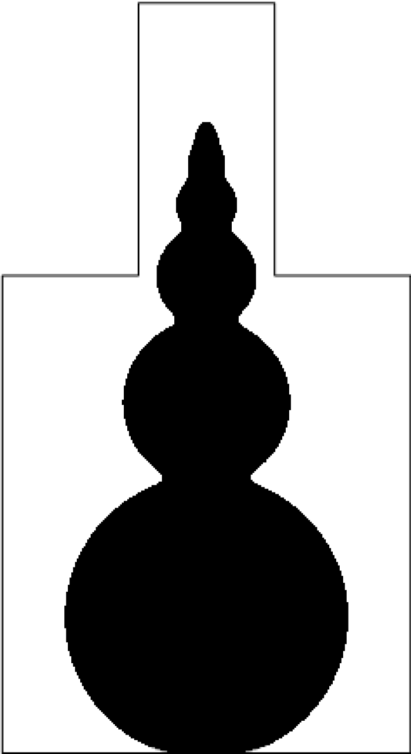
(b) Smoothed set $\widetilde{E}$.

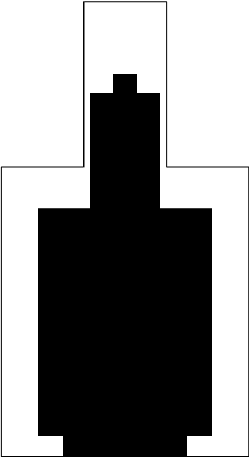
(c) Squared set $\widehat{E}_{0}$.

(d) Aligned set $F$.

Figure 3: The construction in Lemma 2 applied to an example set of finite perimeter contained in a rectilinear polygon (in case $f=0$).

Step 3. Aligning
Take any line $L_{0}\subset G(\widehat{E}_{0})$ that is not contained in $G$. We assume for clarity that $L$ is horizontal, i. e. $L=\mathbb{R}\times\{y_{0}\}$, $y_{0}\in\mathbb{R}$. We denote $L_{0}\cap\partial\widehat{E}_{0}=C_{0}\times\{y_{0}\}$ and observe that $C_{0}\subset\mathbb{R}$ necessarily contains an interval. Let $L_{+}=\mathbb{R}\times\{y_{+}\}$ and $L_{-}=\mathbb{R}\times\{y_{-}\}$ be the lines in $G\cup G(\widehat{E}_{0})$ situated above and below $L_{0}$ closest to $L_{0}$. We have $C_{0}\times[y_{-},y_{+}]\subset F_{0}$. Let us first assume that $\widehat{E}_{0}\neq C_{0}\times[y_{0},y_{+}]$, $\widehat{E}_{0}\neq C_{0}\times[y_{-},y_{0}]$. For $y\in[y_{-},y_{+}]$, we define

$$\overline{\mathcal{J}}(y)=\left\{\begin{array}[]{ll}\mathcal{J}(\widehat{E}_{0}\,\triangle\,(C_{0}\times[y_{0},y]))&\text{if }y>y_{0},\\ \mathcal{J}(\widehat{E}_{0}\,\triangle\,(C_{0}\times[y,y_{0}]))&\text{otherwise.}\end{array}\right.$$ (24)

Denoting $\mathcal{Q}_{f}=\{Q_{1},\ldots,Q_{n}\}$, we observe that $Q_{i}\cap(C_{0}\times[y_{-},y_{+}])=C_{i}\times[y_{-},y_{+}]$ with $C_{i}\subset\mathbb{R}$ for $i=1,\ldots,n$. This follows from the choice of $L_{0}$ and $L_{\pm}$. Similarly, each one of line segments constituting $\partial C_{0}\times[y_{-},y_{+}]$ is contained (up to a finite number of points) in $\partial F_{+}\cup\mathrm{int}\,F$, $\partial F_{-}$ or $\partial F\setminus(\partial F^{+}\cup\partial F^{-})$. Therefore, $\overline{\mathcal{J}}$ is a homography and hence monotone on $]y_{-},y_{+}[$.

However, $\overline{\mathcal{J}}$ might be discontinuous at the endpoints of its domain. This is only possible if, as $y$ attains $y_{+}$ (or $y_{-}$), a pair of edges of $\widehat{E}_{0}\,\triangle\,(C_{0}\times[y_{0},y])$ (resp. $\widehat{E}_{0}\,\triangle\,(C_{0}\times[y,y_{0}])$) vanishes, or an edge touches the boundary of $F_{0}$. In either case, there still holds $\lim_{y\to y_{\pm}}\overline{\mathcal{J}}(y)\geq\overline{\mathcal{J}}(y_{\pm})$.

Thus, whether $\overline{\mathcal{J}}$ is continuous or not, either $\overline{\mathcal{J}}(y_{+})$ or $\overline{\mathcal{J}}(y_{-})$ (or both) is not larger than $\overline{\mathcal{J}}(y_{0})=\mathcal{J}(\widehat{E}_{0})$. In accordance with that, we denote either $\widehat{E}_{1}=\widehat{E}_{0}\,\triangle\,(C_{0}\times[y_{0},y_{+}])$ or $\widehat{E}_{1}=\widehat{E}_{0}\,\triangle\,(C_{0}\times[y_{-},y_{0}])$ and perform the same argument with $\widehat{E}_{1}$ instead of $\widehat{E}_{0}$.

Now, let us go back to the excluded cases and suppose, without loss of generality, that $\widehat{E}_{0}=C_{0}\times[y_{0},y_{+}]$. Then, $\overline{\mathcal{J}}$ is still a well-defined homography in $[y_{-},y_{+}[$ and $\lim_{y\to y_{+}}\overline{\mathcal{J}}(y)=+\infty$. Hence, $\overline{\mathcal{J}}(y_{-})\leq\overline{\mathcal{J}}(y_{0})=\mathcal{J}(\widehat{E}_{0})$ and we put $\widehat{E}_{1}=\widehat{E}_{0}\,\triangle\,(C_{0}\times[y_{-},y_{0}])=C_{0}\times[y_{-},y_{+}]$ and continue the procedure.

For each $i$, $G(\widehat{E}_{i+1})$ contains at least one line not contained in $G$ less than $G(\widehat{E}_{i})$, so this procedure terminates in a finite number $s$ of steps and we obtain $F=\widehat{E}_{s}$ whose all edges are contained in $G$ and $\mathcal{J}(F)\leq\mathcal{J}(\widehat{E}_{0})<\mathcal{J}(E)+\varepsilon$. ∎

Theorem 3.

The functional $\mathcal{J}_{F_{0},\partial F_{0}^{+},\partial F_{0}^{-},f}$ is bounded from below and is minimized by a rectilinear polygon $F\subset F_{0}$ such that $F\in\mathcal{F}(G)$.

Proof.

Suppose that $\mathcal{J}_{F_{0},\partial F_{0}^{+},\partial F_{0}^{-},f}(E_{n})\to-\infty$. Then, due to Lemma 2 there exist rectilinear polygons $F_{n}\subset F_{0}$, $n=1,2,\ldots$ such that $F_{n}\in\mathcal{F}(G)$ and $\mathcal{J}_{F_{0},\partial F_{0}^{+},\partial F_{0}^{-},f}(F_{n})\to-\infty$, an impossibility.

Now, consider any minimizing sequence $(E_{n})$ of $\mathcal{J}_{F_{0},\partial F_{0}^{+},\partial F_{0}^{-},f}$. By means of Lemma 2 we find a minimizing sequence of rectilinear polygons $F_{n}\in F_{0}$ such that $F\in\mathcal{F}(G)$. As the set of such rectilinear polygons is finite, $(F_{n})$ has a constant subsequence $(F_{n_{k}})\equiv(F)$. Clearly, $F$ minimizes $\mathcal{J}_{F_{0},\partial F_{0}^{+},\partial F_{0}^{-},f}$. ∎

Instead of $\mathcal{J}_{F_{0},\partial F_{0}^{+},\partial F_{0}^{-},f}$ we can consider

$$\check{\mathcal{J}}_{F_{0},\partial F_{0}^{+},\partial F_{0}^{-},f}(E)\colon\{E\subset F_{0}\text{ --- measurable s.\,t. }\mathcal{L}^{2}(E)>0\}\to[-\infty,+\infty[$$

defined by

$$\check{\mathcal{J}}_{F_{0},\partial F_{0}^{+},\partial F_{0}^{-},f}(E)=\frac{-{\rm Per}_{1}(E,\mathrm{int}\,F_{0})+\mathcal{H}^{1}(\partial^{*}E\cap\partial F_{0}^{+})-\mathcal{H}^{1}(\partial^{*}E\cap\partial F_{0}^{-})-\int_{E}f\,\mathrm{d}\mathcal{L}^{2}}{\mathcal{L}^{2}(E)},$$

if $E$ has finite perimeter and $-\infty$ otherwise. Then, noticing that

$$\check{\mathcal{J}}_{F_{0},\partial F_{0}^{+},\partial F_{0}^{-},f}=-\mathcal{J}_{F_{0},\partial F_{0}^{-},\partial F_{0}^{+},-f}$$

we obtain analogous versions of Lemma 2 and Theorem 3.

Lemma 3.

Let $E\subset F_{0}$ be a set of finite perimeter with $\mathcal{L}^{2}(E)>0$. Then for every $\varepsilon>0$ there exists a rectilinear polygon $F\in\mathcal{F}(G)$ such that

$$\check{\mathcal{J}}_{F_{0},\partial F_{0}^{+},\partial F_{0}^{-},f}(F)>\check{\mathcal{J}}_{F_{0},\partial F_{0}^{+},\partial F_{0}^{-},f}(E)-\varepsilon.$$

Theorem 4.

The functional $\check{\mathcal{J}}_{F_{0},\partial F_{0}^{+},\partial F_{0}^{-},f}$ is bounded from above and is maximized by a rectilinear polygon $F\subset F_{0}$ such that $F\in\mathcal{F}(G)$.

4 The minimization problem for $TV_{1}$ with $PCR$ datum

Let $\Omega$ be a rectilinear polygon and let $u_{0}$ belong to $PCR(\Omega)$. Given $\lambda>0$, we use Lemma 3 to prove that the solution $u$ to the problem (4) is encoded in the partition $\{F_{1},\ldots,F_{l}\}$ of $\Omega$ (partition into level sets of $u$) and consistent signature $F_{k}\mapsto(\partial F_{k}^{+},\partial F_{k}^{-})$, $k=1,\ldots,l$ (signature induced by $u$), both subordinate to $G_{u_{0}}$, produced by the following algorithm:

• First, denote by $F_{1}$ the largest minimizer of $\mathcal{J}_{\Omega,\emptyset,\emptyset,\frac{u_{0}}{\lambda}}$, and put $\partial F_{1}^{+}=\partial F_{1}\setminus\partial\Omega$, $\partial F_{1}^{-}=\emptyset$.

• At $k$-th step, denote $\check{F}_{k}=\bigcup_{i=1}^{k-1}F_{i}$. If $\Omega=\check{F}_{k}$, stop. Otherwise, denote by $F_{k}$ the largest minimizer of $\mathcal{J}_{\Omega\setminus\check{F}_{k},\emptyset,\partial\check{F}_{k},\frac{u_{0}}{\lambda}}$ and put $\partial F_{k}^{+}=\partial F_{k}\setminus(\partial\Omega\cup\partial\check{F}_{k})$, $\partial F_{k}^{-}=\partial F_{k}\cap\partial\check{F}_{k}$.

We take the largest minimizer, because we want to construct the whole level set in one turn. As Cheeger quotients are subadditive, the largest minimizer is the sum of all minimizers. Note that the algorithm ends after a finite number of steps, as $\check{F}_{k}$ is larger than $\check{F}_{k-1}$ by $F_{k}$, a non-empty rectilinear polygon subordinate to $G(u_{0})$ and contained in $\Omega$. These collectively make a finite set.

Remark.

$\partial F_{k}^{\pm}$ are defined in such a way that each $\mathcal{J}_{F_{k},\partial F_{k}^{+},\partial F_{k}^{-},\frac{u_{0}}{\lambda}}$ is the restriction of $\mathcal{J}_{\Omega\setminus\check{F}_{k},\emptyset,\partial\check{F}_{k},\frac{u_{0}}{\lambda}}$ to subsets of $F_{k}$. In particular, $F_{k}$ is a minimizer of $\mathcal{J}_{F_{k},\partial F_{k}^{+},\partial F_{k}^{-},\frac{u_{0}}{\lambda}}$.

Theorem 5.

Let $F_{k}$, $(\partial F_{k}^{+},\partial F_{k}^{-})$, $k=1,\ldots,l$ be as above. Let $u\in PCR(\Omega)$ be given by

$$u|_{F_{k}}=\frac{1}{\mathcal{L}^{2}(F_{k})}\left(\int_{F_{k}}u_{0}\,\mathrm{d}\mathcal{L}^{2}-\lambda(\mathcal{H}^{1}(\partial F_{k}^{+})-\mathcal{H}^{1}(\partial F_{k}^{-}))\right)$$ (25)

for $k=1,\ldots,l$. Then $u$ is the solution to (4). Furthermore, $\mathcal{Q}_{u}=\{F_{1},\ldots,F_{l}\}$, $\mathcal{S}_{u}(F_{k})=(\partial F_{k}^{+},\partial F_{k}^{-})$, $k=1,\ldots,l$.

Proof.

We now adapt the reasoning in the proof of Theorem 5 in [5]. For given $k=1,\ldots,l$, we consider the functional $\mathcal{F}_{k}$ defined by

$$\mathcal{F}_{k}(\boldsymbol{\xi})=\int_{F_{k}}\left(\mathrm{div}\,\boldsymbol{\xi}+\frac{u_{0}}{\lambda}\right)^{2}\,\mathrm{d}\mathcal{L}^{2}$$

on the set of vector fields $\boldsymbol{\eta}\in X_{F_{k}}$ satisfying

$$|\boldsymbol{\eta}|_{\infty}\leq 1\qquad\left.[\boldsymbol{\eta},\boldsymbol{\nu}^{F_{k}}]\right|_{\partial F_{k}^{\pm}}=\mp 1,\qquad\left.[\boldsymbol{\eta},\boldsymbol{\nu}^{F_{k}}]\right|_{\partial F_{k}\cap\partial\Omega}=0.$$

We first prove that any vector field $\boldsymbol{\xi}\in L^{\infty}(\Omega,{\mathbb{R}^{2}})$, such that $\boldsymbol{\xi}|_{F_{k}}$ satisfies above conditions for each $k=1,\ldots,l$, belongs to $X_{1,\Omega}(u)$, with $u$ defined by (25). This follows immediately by Lemma 1 once we know that $F_{k}\mapsto(\partial F_{k}^{+},\partial F_{k}^{-})$, $k=1,\ldots,l$ is the signature induced by $u$, i. e. that the inequality

$$\frac{1}{\mathcal{L}^{2}(F_{k+1})}\left(\int_{F_{k+1}}u_{0}\,\mathrm{d}\mathcal{L}^{2}-\lambda(\mathcal{H}^{1}(\partial F_{k+1}\setminus(\partial\Omega\cup\partial\check{F}_{k+1}))-\mathcal{H}^{1}(\partial F_{k+1}\cap\partial\check{F}_{k+1}))\right)=u|_{F_{k+1}}\\ <u|_{F_{k}}=\frac{1}{\mathcal{L}^{2}(F_{k})}\left(\int_{F_{k}}u_{0}\,\mathrm{d}\mathcal{L}^{2}-\lambda(\mathcal{H}^{1}(\partial F_{k}\setminus(\partial\Omega\cup\partial\check{F}_{k}))-\mathcal{H}^{1}(\partial F_{k}\cap\partial\check{F}_{k}))\right),$$ (26)

is satisfied for $k=1,\ldots,l-1$ with $u$ defined in (25). Note that we have

$$\mathcal{H}^{1}(\partial F_{k+1}\cap\partial\check{F}_{k})=\mathcal{H}^{1}(\partial F_{k+1}\cap\partial\check{F}_{k+1})-\mathcal{H}^{1}(\partial F_{k+1}\cap\partial F_{k})\\ \text{and}\quad\mathcal{H}^{1}(\partial F_{k+1}\setminus(\partial\Omega\cup\check{F}_{k}))=\mathcal{H}^{1}(\partial F_{k+1}\setminus(\partial\Omega\cup\check{F}_{k+1}))+\mathcal{H}^{1}(\partial F_{k+1}\cap\partial F_{k}).$$

Thus, were (26) not the case, we would have (using the inequality $\frac{x_{1}+x_{2}}{y_{1}+y_{2}}\leq\frac{x_{1}}{y_{1}}$ that holds whenever $\frac{x_{2}}{y_{2}}\leq\frac{x_{1}}{y_{1}}$ for positive numbers $x_{1},x_{2},y_{1},y_{2}$),

$$\mathcal{J}_{\Omega\setminus\check{F}_{k},\emptyset,\partial\check{F}_{k},\frac{u_{0}}{\lambda}}(F_{k}\cup F_{k+1})\\ \leq\frac{1}{\mathcal{L}^{2}(F_{k})+\mathcal{L}^{2}(F_{k+1})}\left(\mathcal{H}^{1}(\partial F_{k}\cap\partial\check{F}_{k})-\mathcal{H}^{1}(\partial F_{k}\setminus(\partial\Omega\cup\partial\check{F}_{k}))-\frac{1}{\lambda}\int_{F_{k}}u_{0}\,\mathrm{d}\mathcal{L}^{2}\right.\\ \left.+\mathcal{H}^{1}(\partial F_{k+1}\cap\partial\check{F}_{k+1})-\mathcal{H}^{1}(\partial F_{k+1}\setminus(\partial\Omega\cup\partial\check{F}_{k+1}))-\frac{1}{\lambda}\int_{F_{k+1}}u_{0}\,\mathrm{d}\mathcal{L}^{2}\right)\\ \leq\mathcal{J}_{\Omega\setminus\check{F}_{k},\emptyset,\partial\check{F}_{k},\frac{u_{0}}{\lambda}}(F_{k}),$$ (27)

in contradiction with the choice of $F_{k}$.

Proceeding as in [6, Proposition 6.1], we see that $\mathcal{F}_{k}$ attains a minimum and for any two minimizers $\boldsymbol{\eta}_{1},\boldsymbol{\eta}_{2}$ we have $\mathrm{div}\,\boldsymbol{\eta}_{1}=\mathrm{div}\,\boldsymbol{\eta}_{2}$ in $F_{k}$. Let us take any minimizer and denote it $\boldsymbol{\xi}_{F_{k}}$. Arguing as in [6, Theorem 6.7] and [7, Theorem 5.3], $\mathrm{div}\,\boldsymbol{\xi}_{F_{k}}\in L^{\infty}(F_{k})\cap BV(F_{k})$. Let $\nu=\mathcal{J}_{F_{k},\partial F_{k}^{+},\partial F_{k}^{-},\frac{u_{0}}{\lambda}}(F_{k})$. We have

$$\frac{1}{\mathcal{L}^{2}(F_{k})}\int_{F_{k}}\left(\mathrm{div}\,\boldsymbol{\xi}_{F_{k}}+\frac{u_{0}}{\lambda}\right)\,\mathrm{d}\mathcal{L}^{2}=-\frac{1}{\mathcal{L}^{2}(F_{k})}\left(\mathcal{H}^{1}(\partial F_{k}^{+})-\mathcal{H}^{1}(\partial F_{k}^{-})-\frac{1}{\lambda}\int_{F_{k}}u_{0}\,\mathrm{d}\mathcal{L}^{2}\right)=-\nu.$$

Were $\mathrm{div}\,\boldsymbol{\xi}_{F_{k}}+\frac{u_{0}}{\lambda}$ not constant in $F_{k}$, there would exist $\mu<\nu$ such that

$$A_{\mu}=\left\{\boldsymbol{x}\in F_{k}\colon-\left(\mathrm{div}\,\boldsymbol{\xi}_{F_{k}}(\boldsymbol{x})+\frac{u_{0}}{\lambda}\right)<\mu\right\}$$

has positive measure and finite perimeter. Employing [7, Proposition 3.5],

$$-\nu<-\mu<\frac{1}{\mathcal{L}^{2}(A_{\mu})}\int_{A_{\mu}}\left(\mathrm{div}\,\boldsymbol{\xi}_{F_{k}}+\frac{u_{0}}{\lambda}\right)\,\mathrm{d}\mathcal{L}^{2}\\ =-\frac{1}{\mathcal{L}^{2}(A_{\mu})}\left(\mathrm{Per}_{1}(A_{\mu},F_{k})+\mathcal{H}^{1}(\partial F_{k}^{+}\cap\partial^{*}A_{\mu})-\mathcal{H}^{1}(\partial F_{k}^{-}\cap\partial^{*}A_{\mu})-\frac{1}{\lambda}\int_{F_{k}}u_{0}\,\mathrm{d}\mathcal{L}^{2}\right)\\ =-\mathcal{J}_{F_{k},\partial F_{k}^{+},\partial F_{k}^{-},\frac{u_{0}}{\lambda}}(A_{\mu}),$$

which would contradict that $F_{k}$ minimizes $\mathcal{J}_{F_{k},\partial F_{k}^{+},\partial F_{k}^{-},\frac{u_{0}}{\lambda}}$ (see the Remark before the statement of the Theorem), hence $u_{0}+\lambda\mathrm{div}\,\boldsymbol{\xi}_{F_{k}}$ is constant in $F_{k}$ and therefore equal to its mean value:

$$u_{0}+\lambda\mathrm{div}\,\boldsymbol{\xi}_{F_{k}}=\frac{1}{\mathcal{L}^{2}(F_{k})}\left(\int_{F_{k}}u_{0}\,\mathrm{d}\mathcal{L}^{2}-\lambda(\mathcal{H}^{1}(\partial F_{k}^{+})-\mathcal{H}^{1}(\partial F_{k}^{-}))\right)=u,$$

i. e. $u$ satisfies the Euler-Lagrange equation (13).

The last sentence of the assertion follows from (26). ∎

Remark.

Instead of considering the minimization problem for $\mathcal{J}$, one can consider at each step the maximization problem for $\check{\mathcal{J}}$ (see Theorem 4).

5 The $TV_{1}$ flow with $PCR$ initial datum

In what now follows, we are concerned with the identification of the evolution of initial datum $w\in PCR(\Omega)$, with $\Omega$ a rectilinear polygon, under the $l^{1}$-anisotropic total variation flow (5). The result below determines the initial evolution, prescribing possible breaking of initial facets.

Theorem 6.

Let $w\in PCR(\Omega)$ and let $G$ be any grid such that $\mathcal{Q}_{w}$ is subordinate to $G$. Then, there exists a field $\boldsymbol{\eta}\in X_{1,\Omega}(w)$ and, for each $Q\in\mathcal{Q}_{w}$, a partition $\mathcal{T}_{Q}$ of $Q$ and a consistent signature $\mathcal{S}_{Q}$ for $\mathcal{T}_{Q}$ subordinate to $G$, $\mathcal{S}_{Q}\colon F\mapsto(\partial F^{+},\partial F^{-})$ for $F\in\mathcal{T}_{Q}$, such that

• $\mathcal{T}=\bigcup_{Q\in\mathcal{Q}_{w}}\mathcal{T}_{Q}$ is a partition of $\Omega$ subordinate to $G$, $\mathcal{S}\colon\mathcal{T}\to\mathcal{C}\times\mathcal{C}$ given by $\mathcal{S}(F)=\mathcal{S}_{Q}(F)$ for $F\in\mathcal{T}_{Q}$ is a consistent signature for $\mathcal{T}$ subordinate to $G$,

• for each $F\in\mathcal{T}$,

  $$\left.\mathrm{div}\,\boldsymbol{\eta}\right|_{F}=-\frac{1}{\mathcal{L}^{2}(F)}\left(\mathcal{H}^{1}(\partial F^{+})-\mathcal{H}^{1}(\partial F^{-})\right),\qquad\left.[\boldsymbol{\eta},\boldsymbol{\nu}^{F}]\right|_{\partial F^{\pm}}=\mp 1.$$

Proof.

We fix $Q\in\mathcal{Q}_{w}$ and produce the partition $\mathcal{T}_{Q}$ of $Q$ and consistent signature $\mathcal{S}_{Q}$ for $\mathcal{T}_{Q}$ by means of an inductive procedure analogous to the one in section 4. First, by virtue of Theorem 3, the functional $\mathcal{J}_{Q,\partial Q^{+},\partial Q^{-},0}$ attains its minimum value on a rectilinear polygon $F_{1}\in\mathcal{F}(G)$. We define

$$\partial F_{1}^{-}=\partial Q^{-}\cap\partial F_{1}\mbox{ \ \ and \ \ }\partial F_{1}^{+}=(\partial F_{1}\cap\partial Q^{+})\cup(\partial F_{1}\setminus\partial Q).$$

Next, in $k$-th step, we put $\check{F}_{k}=\bigcup_{j=1}^{k-1}F_{j}$. If $\check{F}_{k}=Q$ we stop and put $\mathcal{T}_{Q}=\{F_{1},\ldots,F_{k-1}\}$, $\mathcal{S}_{Q}(F_{j})=(\partial F_{j}^{+},\partial F_{j}^{-})$ for $j=1,\ldots,k-1$. Otherwise we define $F_{k}$ as any minimizer of

$$\mathcal{J}_{Q\setminus\check{F}_{k},\partial Q^{+},\partial Q^{-}\cup\partial\check{F}_{k},0},$$

and

$$\partial F_{k}^{-}=\partial F_{k}\cap\left(\partial Q^{-}\cup\partial\check{F}_{k}\right),$$

$$\partial F_{k}^{+}=(\partial F_{k}\cap\partial Q^{+})\cup\left(\partial F_{k}\setminus\left(\partial Q\cup\partial\check{F}_{k}\right)\right).$$

Now, for each $F_{k}\in\mathcal{T}_{Q}$, we define $\boldsymbol{\eta}_{F_{k}}$ as any minimizer of the functional $\mathcal{F}_{k}$ defined on the set of vector fields $\boldsymbol{\xi}\in L^{\infty}(F_{k},{\mathbb{R}^{2}})$ satisfying

$$\mathrm{div}\,\boldsymbol{\xi}\in L^{2}(F_{k}),\qquad|\boldsymbol{\xi}|_{\infty}\leq 1\qquad\left.[\boldsymbol{\xi},\boldsymbol{\nu}^{F_{k}}]\right|_{\partial F_{k}^{\pm}}=\mp 1,\qquad\left[\boldsymbol{\xi},\boldsymbol{\nu}^{F_{k}}]\right|_{\partial F_{k}\cap\partial\Omega}=0$$

by $\mathcal{F}_{k}(\boldsymbol{\xi})=\int_{F_{k}}(\mathrm{div}\,\boldsymbol{\xi})^{2}\,\mathrm{d}\mathcal{L}^{2}$. As in the proof of Theorem 5, we prove that $\mathrm{div}\,\boldsymbol{\eta}_{F_{k}}$ is constant in each $F_{k}\in T_{Q}$.

Next, we repeat the procedure for the rest of $Q\in\mathcal{Q}_{w}$ and define $\boldsymbol{\eta}$ by $\boldsymbol{\eta}|_{F_{k}}=\boldsymbol{\eta}_{F_{k}}$ for every $F_{k}\in\mathcal{T}_{Q}$, $Q\in\mathcal{Q}_{w}$. Clearly, $\boldsymbol{\eta}\in X_{1,\Omega}(w)$. ∎

Theorem 7.

Let $u_{0}\in PCR(\Omega)$ and denote $G=G_{u_{0}}$. Let $u$ be the global strong solution to (5). Then there exist a finite sequence of time instances $0=t_{0}<t_{1}<\ldots<t_{n}$, partitions $\mathcal{Q}_{0},\ldots,\mathcal{Q}_{n-1}$ of $\Omega$ and consistent signatures $\mathcal{S}_{k}$ for $\mathcal{Q}_{k}$ subordinate to $G$, $k=0,\ldots,n-1$, such that

$$u_{t}=-\frac{1}{\mathcal{L}^{2}(F)}\left(\mathcal{H}^{1}(\partial F^{+})-\mathcal{H}^{1}(\partial F^{-})\right)\quad\text{in }]t_{k},t_{k+1}[\times F\quad\text{for each }F\in\mathcal{Q}_{k},$$ (28)

$k=0,1,\ldots,n-1$ and $u(t,\cdot)=\frac{1}{\mathcal{L}^{2}(\Omega)}\int_{\Omega}u_{0}\,\mathrm{d}\mathcal{L}^{2}$ for $t\geq t_{n}$. In particular, $u(t,\cdot)\in PCR(\Omega)$ and $\mathcal{Q}_{u(t,\cdot)}$ is subordinate to $G$ for all $t>0$. Furthermore,

$$t_{n}\leq\frac{1}{2}\left(\min_{F\subsetneq\Omega,F\in\mathcal{F}(G)}\frac{\mathrm{Per}_{1}(F,\Omega)}{\mathcal{L}^{2}(F)}\right)^{-1}\cdot\max\left|u_{0}-\frac{1}{\mathcal{L}^{2}(\Omega)}\int_{\Omega}u_{0}\,\mathrm{d}\mathcal{L}^{2}\right|.$$ (29)

Remark.

Theorem 7 implies that $t\mapsto u(t,\cdot)$ has a representative that is Lipschitz with values in $BV(\Omega)$.

Proof.

We proceed inductively, starting with $j=0$. Suppose we have proved that there exist time instances $0=t_{0}<\ldots<t_{j}$, partitions $\mathcal{Q}_{k}$ of $\Omega$ and consistent signatures $\mathcal{S}_{k}$ for $\mathcal{Q}_{k}$ subordinate to $G$, $k=0,\ldots,j-1$, such that (28) holds for $k=1,\ldots,j$ (for $j=0$ this assumption is vacuously satisfied). This implies that $u(t,\cdot)\in PCR(\Omega)$ and $\mathcal{Q}_{u(t,\cdot)}$ is subordinate to $G$ for $t\in[0,t_{j}]$. Let $\mathcal{Q}_{j}=\mathcal{T}$, $\mathcal{S}_{j}=\mathcal{S}$, $\boldsymbol{z}_{j}=\boldsymbol{\eta}$, where $\mathcal{T}$, $\mathcal{S}$ and $\boldsymbol{\eta}$ are the partition of $\Omega$, the consistent signature for $\mathcal{T}$ subordinate to $G$ and the vector field produced by Theorem 6 given $w=u(t_{j},\cdot)$. For $T>0$ let us define a function $\widetilde{u}_{j}\in C([t_{j},T[,BV(\Omega))$ by

$$\widetilde{u}_{j,t}(t,\cdot)=\mathrm{div}\,\boldsymbol{z}_{j}\text{ for }t\in]t_{j},T[,$$

$$\widetilde{u}_{j}(t_{j},\cdot)=u(t_{j},\cdot).$$

Clearly, pair $(\widetilde{u}_{j},\boldsymbol{z}_{j})$ satisfies regularity conditions as well as (16, 17) from Definition 1. Let us choose $T=t_{j+1}$ as the first time instance $t>t_{j}$ such that

$$\widetilde{u}_{j}(t,\cdot)|_{F}=\widetilde{u}_{j}(t,\cdot)|_{F^{\prime}},$$

where $F,F^{\prime}\in\mathcal{Q}_{j}$, $F\neq F^{\prime}$, $\mathcal{H}^{1}(\partial F\cap\partial F^{\prime})>0$; i. e. the first moment of merging of facets after time $t_{j}$.

Due to condition (4) of Theorem 6, one can show, similarly as in the proof of Theorem 5, that condition (19) of Definition 1 is satisfied for $(\widetilde{u}_{j},\boldsymbol{z}_{j})$ and $\widetilde{u}_{j}$ is the solution to (15) with initial datum $u(t_{j},\cdot)$ in $[t_{j},t_{j+1}[$. Then, due to continuity, $u$ is necessarily equal to $\widetilde{u}_{j}$ in $[t_{j},t_{j+1}]$, in particular, for $t\in[t_{j},t_{j+1}]$, $u(t,\cdot)\in PCR(\Omega)$ and $\mathcal{Q}_{u(t,\cdot)}$ is subordinate to $G$. This completes the proof of the induction step.

Now, let us prove that this procedure terminates after a finite number of steps. For this purpose, we rely on Theorem 2. In fact, we prove that there exists a constant $\gamma=\gamma(G)>0$ such that at each $t_{j}$, $j>0$ the non-increasing function $t\mapsto\|\mathrm{div}\,\boldsymbol{z}(t,\cdot)\|_{L^{2}(\Omega)}$ has a jump of size at least $\gamma$. Here $\boldsymbol{z}\in L^{\infty}(]0,\infty[\times\Omega)$ satisfies the conditions in Definition 1 with $u$ being the strong solution to (5) starting with $u_{0}$.

First, we argue that $\|\mathrm{div}\,\boldsymbol{z}(t_{j},\cdot)\|_{L^{2}(\Omega)}<\|\mathrm{div}\,\boldsymbol{z}(t,\cdot)\|_{L^{2}(\Omega)}$ for each $t\in[t_{j-1},t_{j}[$ (in this interval $t\mapsto\mathrm{div}\,\boldsymbol{z}(t,\cdot)$ is a constant function). We will reason by contradiction. If $\|\mathrm{div}\,\boldsymbol{z}(t_{j},\cdot)\|_{L^{2}(\Omega)}=\|\mathrm{div}\,\boldsymbol{z}(t_{j-1},\cdot)\|_{L^{2}(\Omega)}$, then $\boldsymbol{z}(t_{j-1},\cdot)$ is a minimizer of $\mathcal{F}_{\Omega}$ in $X_{1,\Omega}(u(t_{j},\cdot))$ and consequently $\mathrm{div}\,\boldsymbol{z}(t_{j-1},\cdot)=\mathrm{div}\,\boldsymbol{z}(t_{j},\cdot)=\mathrm{div}\,\boldsymbol{z}(t,\cdot)$ for $t\in[t_{j-1},t_{j+1}[$ (see Theorem 2). According to Lemma 1, the minimization problem for $\mathcal{F}_{\Omega}$ in $X_{1,\Omega}(u(t_{j},\cdot))$ is equivalent to minimization of functionals $\mathcal{F}_{Q}$ defined by $\mathcal{F}_{Q}(\boldsymbol{\eta})=\int_{Q}\left(\mathrm{div}\,\boldsymbol{\eta}\right)^{2}\,\mathrm{d}\mathcal{L}^{2}$ on the set of vector fields $\boldsymbol{\eta}\in L^{\infty}(Q,{\mathbb{R}^{2}})$ satisfying

$$\mathrm{div}\,\boldsymbol{\eta}\in L^{2}(Q),\qquad|\boldsymbol{\eta}|_{\infty}\leq 1\qquad\left.[\boldsymbol{\eta},\boldsymbol{\nu}^{Q}]\right|_{\partial Q^{\pm}}=\mp 1,\qquad\left.[\boldsymbol{\eta},\boldsymbol{\nu}^{Q}]\right|_{\partial Q\cap\partial\Omega}=0$$

separately for each $Q\in\mathcal{Q}_{u(t_{j},\cdot)}$, where $(\partial Q^{+},\partial Q^{+})=\mathcal{S}_{u(t_{j},\cdot)}(Q)$. Let us take $Q\in\mathcal{Q}_{u(t_{j},\cdot)}$ such that there exist $F_{1},F_{2}$ in $\mathcal{Q}_{j-1}$, $F_{1}\neq F_{2}$, $\mathcal{H}^{1}(\partial F_{1}\cap\partial F_{2})>0$, with $F_{1},F_{2}\subset Q$. Denote by $\mathcal{Q}_{j-1,Q}$ the maximal subset of $\mathcal{Q}_{j-1}$ with the properties

• $F_{1},F_{2}$ belong to $\mathcal{Q}_{j-1,Q}$,

• if $F$ belongs to $\mathcal{Q}_{j-1}$ then $F\subset Q$,

• if $F$ belongs to $\mathcal{Q}_{j-1,Q}$ then there exists $F^{\prime}\in\mathcal{Q}_{j-1,Q}$, $F^{\prime}\neq F$ with $\mathcal{H}^{1}(\partial F\cap\partial F^{\prime})\neq 0$.

Let now $F_{0}$ be a minimizer of $F\mapsto u_{t}|_{]t_{j-1},t_{j+1}[\times F}=\mathrm{div}\,\boldsymbol{z}|_{]t_{j-1},t_{j+1}[\times F}$ among $F\in\mathcal{Q}_{j-1,Q}$. Then, due to (19) and the way $Du$ changes after the moment of merging, we necessarily have

$$\left.[\boldsymbol{z},\boldsymbol{\nu}^{F_{0}}]\right|_{]t_{j},t_{j+1}[\times\partial F_{0}^{-}\cup(\partial F_{0}^{+}\setminus\partial Q)}=+1.$$

Due to the choice of $F_{0}$, $\mathcal{H}^{1}(\partial F_{0}^{+}\setminus\partial Q)>0$, hence

$$\left.\frac{1}{\mathcal{L}^{2}(F_{0})}\int_{F_{0}}\mathrm{div}\,\boldsymbol{z}\,\mathrm{d}\mathcal{L}^{2}\right|_{[t_{j},t_{j+1}[}>\left.\frac{1}{\mathcal{L}^{2}(F_{0})}\int_{F_{0}}\mathrm{div}\,\boldsymbol{z}\,\mathrm{d}\mathcal{L}^{2}\right|_{[t_{j-1},t_{j}[},$$

a desired contradiction.

Next, we observe that there is only a finite set of values, depending only on $G$, that $\|\mathrm{div}\,\boldsymbol{z}(t,\cdot)\|_{L^{2}(\Omega)}$ can achieve. Indeed, for all $t\geq 0$, $\mathrm{div}\,\boldsymbol{z}(t,\cdot)$ is the unique result of minimization problems for $\mathcal{F}_{Q}$ with $Q\in\mathcal{Q}_{u(t_{j},\cdot)}$, $(\partial Q^{+},\partial Q^{-})=\mathcal{S}_{u(t_{j},\cdot)}(Q)$, $j=0,1,\ldots$. Each $\mathcal{Q}_{u(t_{j},\cdot)}$ is a partition of $\Omega$ subordinate to $G$, each $\mathcal{S}_{u(t_{j},\cdot)}$ is a consistent signature for $\mathcal{Q}_{u(t_{j},\cdot)}$ subordinate to $G$. There is only a finite number of these.

It remains to prove the estimate on $t_{n}$. In any time instance $t\geq 0$ the maximum (minimum) value of $u(t,\cdot)$ is attained in a rectilinear polygon $F_{+}(t)$ ($F_{-}(t)$). In all but a finite number of $t$ we have

$$\mp u_{t}(t,\cdot)|_{F_{\pm}(t)}=\mp\mathrm{div}\,\boldsymbol{z}(t,\cdot)|_{F_{\pm}(t)}=\frac{{\rm Per}_{1}(F_{\pm}(t),\Omega)}{\mathcal{L}^{2}(F_{\pm}(t))}\geq\min_{F\subsetneq\Omega,F\in\mathcal{F}(G)}\frac{\mathrm{Per}_{1}(F,\Omega)}{\mathcal{L}^{2}(F)},$$

unless $F^{+}=F^{-}=\Omega$. Furthermore, testing (15) with $\chi_{\Omega}$ yields $\frac{\,\mathrm{d}}{\,\mathrm{d}t}\int_{\Omega}u(t,\cdot)\,\mathrm{d}\mathcal{L}^{2}=0$ in a. e. $t\geq 0$ and, due to continuity of the semigroup in $L^{2}$,

$$\frac{1}{|\Omega|}\int_{\Omega}u(t,\cdot)\,\mathrm{d}\mathcal{L}^{2}=\frac{1}{|\Omega|}\int_{\Omega}u_{0}\,\mathrm{d}\mathcal{L}^{2}$$

in all $t>0$. This concludes the proof. ∎

6 The case $\Omega={\mathbb{R}^{2}}$

In this section we transfer previous results to the case $\Omega={\mathbb{R}^{2}}$. First, we note that all the definitions and theorems in subsections 2.6 and 2.7 carry over without change (the Neumann boundary condition becomes void) to this case (see [28]). As for the definitions in subsections 2.3, it turns out that the statements of our results transfer nicely to the case of the whole plane if we allow for certain unbounded rectilinear polygons. Accordingly, in this section a subset $F\subset{\mathbb{R}^{2}}$ will be called a rectilinear polygon if either

• $F=\bigcup\mathcal{R}_{F}$ with a finite $\mathcal{R}_{F}\subset\mathcal{R}$ (in which case we say that $F$ is a bounded rectilinear polygon)

• or $F=\overline{{\mathbb{R}^{2}}\setminus\bigcup\mathcal{R}_{F}}$ with a finite $\mathcal{R}_{F}\subset\mathcal{R}$ (in which case we say that $F$ is an unbounded rectilinear polygon).

Next, we restrict ourselves to non-negative compactly supported initial data. We say that a non-negative compactly supported function $w\in BV({\mathbb{R}^{2}})$ belongs to $PCR_{+}({\mathbb{R}^{2}})$ if there exists a partition $\mathcal{Q}$ of ${\mathbb{R}^{2}}$ such that $w$ is constant in the interior of each $Q\in\mathcal{Q}$. Note that any such $\mathcal{Q}$ contains exactly one unbounded set $Q_{0}$ and $w|_{Q_{0}}=0$.

The essential difficulty in obtaining results analogous to Theorems 5 and 7 lies in dealing with unbounded sets that one expects to be produced by a suitable version of the algorithm in Section 4. For this purpose, we need the following

Lemma 4.

Let $f\in PCR_{+}({\mathbb{R}^{2}})$ and let $F$ be an unbounded rectilinear polygon. Then, there exists a vector field $\boldsymbol{\xi}_{F}\in X_{F}$ such that

$$|\boldsymbol{\xi}_{F}|_{\infty}\leq 1,\qquad\mathrm{div}\,\boldsymbol{\xi}_{F}+f|_{F}=\text{const.},\qquad\quad[\boldsymbol{\xi}_{F},\boldsymbol{\nu}^{F}]=1$$ (30)

if and only if

$$\mathcal{H}^{1}(\partial^{*}E\cap\partial F)+\int_{E}f\,\mathrm{d}\mathcal{L}^{2}\leq{\rm Per}_{1}(E,\mathrm{int}\,F)$$ (31)

for all $E\subset F$ bounded of finite perimeter. Moreover, in this case $\mathrm{div}\,\boldsymbol{\xi}_{F}+f=0$ in $F$ for any vector field $\boldsymbol{\xi}_{F}$ satisfying (30).

This is a version of [5, Theorem 5 and Lemma 6] where analogous statement is proved for isotropic perimeter in case $f=0$. The idea of the proof is to consider auxiliary problem in a large enough ball. The proof of Lemma 4 follows along similar lines, however we decided to put it here, also because it seems that there is a small gap in the proof of [5, Theorem 5] that we patch. Namely the first inequality in line 12, page 511 of [5] (corresponding to (36) here) does not seem to be satisfied in general.

Proof.

It is easy to see that if $\boldsymbol{\xi}_{F}$ satisfies (30) then $\mathrm{div}\,\boldsymbol{\xi}_{F}+f=0$ in $F$ (see [5, Lemma 6]). Thus, if a vector field $\boldsymbol{\xi}_{F}\in X_{F}$ satisfies (30), then we have for any bounded set $E\subset{\mathbb{R}^{2}}$ of finite perimeter

$$0=\int_{E}\mathrm{div}\,\boldsymbol{\xi}_{F}+f\,\mathrm{d}\mathcal{L}^{2}\geq\mathcal{H}^{1}(\partial^{*}E\cap\partial F)+\int_{E}f\,\mathrm{d}\mathcal{L}^{2}-{\rm Per}_{1}(E,\mathrm{int}\,F).$$

Now assume that (31) holds. Let us take $R>0$ large enough that

$$2\,\mathrm{dist}(\partial B_{\infty}(R),\partial F\cup\mathrm{supp}\,f)\geq\mathcal{H}^{1}(\partial F)+\int_{F}f\,\mathrm{d}\mathcal{L}^{2}.$$ (32)

Put $c(R)=-\frac{\mathcal{H}^{1}(\partial F)+\int_{F}f\,\mathrm{d}\mathcal{L}^{2}}{\mathcal{H}^{1}(\partial B_{\infty}(R))}$. Denote by $\boldsymbol{\xi}_{R}$ the minimizer of functional $\mathcal{F}$ defined by $\mathcal{F}(\boldsymbol{\eta})=\int_{F\cap B_{\infty}(R)}\left(\mathrm{div}\,\boldsymbol{\eta}+f\right)^{2}\,\mathrm{d}\mathcal{L}^{2}$ on the set of vector fields $\boldsymbol{\eta}\in X_{F\cap B_{\infty}(R)}$ satisfying

$$|\boldsymbol{\eta}|_{\infty}\leq 1,\qquad[\boldsymbol{\eta},\boldsymbol{\nu}^{F}]=1,\qquad[\boldsymbol{\eta},\boldsymbol{\nu}^{B_{\infty}(R)}]=c(R).$$

If $\mathrm{div}\,\boldsymbol{\xi}_{R}+f$ is constant in $F\cap B_{\infty}(R)$ then, due to choice of $c(R)$, $\mathrm{div}\,\boldsymbol{\xi}_{R}+f\equiv 0$ in $F\cap B_{\infty}(R)$. Supposing that the opposite is true, we obtain, as in the proof of Theorem 5, that there exists $\lambda>0$ such that

$$Q_{\lambda}=\{\boldsymbol{x}\in F\cap B_{\infty}(R)\colon\mathrm{div}\,\boldsymbol{\xi}_{R}+f>\lambda\}$$

is a set of positive measure and finite perimeter, and we have

$$-{\rm Per}_{1}(Q_{\lambda},\mathrm{int}\,F\cap B_{\infty}(R))+\mathcal{H}^{1}(\partial^{*}Q_{\lambda}\cap\partial F)+\int_{Q_{\lambda}}f\,\mathrm{d}\mathcal{L}^{2}+c(R)\mathcal{H}^{1}(\partial^{*}Q_{\lambda}\cap\partial B_{\infty}(R))\\ \geq\lambda\mathcal{L}^{2}(Q_{\lambda})>0$$ (33)

which can be rewritten as

$$-{\rm Per}_{1}(Q_{\lambda})+2\mathcal{H}^{1}(\partial^{*}Q_{\lambda}\cap\partial F)+\int_{Q_{\lambda}}f\,\mathrm{d}\mathcal{L}^{2}+(1+c(R))\mathcal{H}^{1}(\partial^{*}Q_{\lambda}\cap\partial B_{\infty}(R))>0.$$ (34)

Assumption (32) implies that $c(R)>-1$, so we approximate $Q_{\lambda}$ with a closed smooth set as in the proof of Lemma 2 in such a way that (34) still holds. Due to additivity of left hand side of (34), there is a connected component $\widetilde{Q}_{\lambda}$ of this smooth set that also satisfies (34), or equivalently

$$-{\rm Per}_{1}(\widetilde{Q}_{\lambda},\mathrm{int}\,F\cap B_{\infty}(R))+\mathcal{H}^{1}(\partial\widetilde{Q}_{\lambda}\cap\partial F)+\int_{\widetilde{Q}_{\lambda}}f\,\mathrm{d}\mathcal{L}^{2}+c(R)\mathcal{H}^{1}(\partial\widetilde{Q}_{\lambda}\cap\partial B_{\infty}(R))>0.$$ (35)

If $\partial\widetilde{Q}_{\lambda}\cap\partial B_{\infty}(R)=\emptyset$, (35) contradicts (31). On the other hand, if $\partial\widetilde{Q}_{\lambda}\cap(\partial F\cup\mathrm{supp}\,f)=\emptyset$, (35) itself is a contradiction (recall that $c(R)\leq 0$). Taking these observations into account, there necessarily holds

$${\rm Per}_{1}(\widetilde{Q}_{\lambda},\mathrm{int}\,F\cap B_{\infty}(R))\geq 2\,\mathrm{dist}(\partial B_{\infty}(R),\partial F\cup\mathrm{supp}\,f),$$ (36)

whence (32) yields a contradiction, unless $\widetilde{Q}_{\lambda}$ is not simply connected in such a way that there is a connected component $\Gamma$ of $\partial\widetilde{Q}_{\lambda}$ such that

• $\widetilde{Q}_{\lambda}$ is inside of $\Gamma$ ($\Gamma$ is the exterior boundary of $\widetilde{Q}_{\lambda}$),

• $\Gamma$ does not intersect $\partial F\cup\mathrm{supp}\,f$,

• and $\Gamma$ intersects all four sides of $B_{\infty}(R)$.

In this case, let us denote by $\widehat{Q}_{\lambda}$ the union of $\widetilde{Q}_{\lambda}$ and the region between $\Gamma$ and $\partial B_{\infty}(R)$. We have $\int_{\Gamma\setminus\partial B_{\infty}(R)}|\boldsymbol{\nu}^{\widetilde{Q}_{\lambda}}|_{1}\,\mathrm{d}\mathcal{H}^{1}\geq\mathcal{H}^{1}(B_{\infty}(R)\setminus\Gamma)$ and consequently (as $-c(R)<1$)

$${\rm Per}_{1}(\widetilde{Q}_{\lambda},\mathrm{int}\,F\cap B_{\infty}(R))-c(R)\mathcal{H}^{1}(\partial\widetilde{Q}_{\lambda}\cap\partial B_{\infty}(R))\geq{\rm Per}_{1}(\widehat{Q}_{\lambda},\mathrm{int}\,F\cap B_{\infty}(R))\\ -c(R)\mathcal{H}^{1}(\partial\widehat{Q}_{\lambda}\cap\partial B_{\infty}(R))={\rm Per}_{1}(\widehat{Q}_{\lambda},\mathrm{int}\,F\cap B_{\infty}(R))+\mathcal{H}^{1}(\partial F)+\int_{F}f\,\mathrm{d}\mathcal{L}^{2},$$

a contradiction with (35) which implies that $\mathrm{div}\,\boldsymbol{\xi}_{R}\equiv 0$. Now, we define $\boldsymbol{\xi}_{F}\in X_{F}$ by

$$\boldsymbol{\xi}_{F}(x_{1},x_{2})=\left\{\begin{array}[]{ll}\boldsymbol{\xi}_{R}(x_{1},x_{2})&\text{in }F\cap B_{\infty}(R),\\ (c(R)\mathrm{sgn}\,x_{1},0)&\text{in }\{|x_{1}|>R,|x_{2}|<R\}\\ (0,c(R)\mathrm{sgn}\,x_{2})&\text{in }\{|x_{1}|<R,|x_{2}|>R\}\\ (0,0)&\text{in }\{|x_{1}|>R,|x_{2}|>R\}.\\ \end{array}\right.$$ (37)

∎

Now given $\lambda>0$, $u_{0}\in PCR_{+}({\mathbb{R}^{2}})$, grid $G=G_{f}$, and an unbounded rectilinear polygon $F$ subordinate to $G$ with signature $(\partial F^{+},\partial F^{-})=(\emptyset,\partial F)$, let us denote by $R_{0}$ the smallest rectangle containing the support of $u_{0}$ (clearly $R_{0}$ is subordinate to $G$ and $\partial F\subset R_{0}$). Next, suppose that there is a set of finite perimeter $E\subset F$ such that $\mathcal{J}_{F,\partial F^{+},\partial F^{-},\frac{u_{0}}{\lambda}}(E)<0$. Then there holds $\mathcal{J}_{F,\partial F^{+},\partial F^{-},\frac{u_{0}}{\lambda}}(R_{0}\cap E)\leq\mathcal{J}_{F,\partial F^{+},\partial F^{-},\frac{u_{0}}{\lambda}}(E)$. Indeed, we only need to argue that ${\rm Per}_{1}(R_{0}\cap E)\leq{\rm Per}_{1}(E)$, which follows easily by approximation of $E$ with smooth sets. This way, we obtain the following alternative:

• either $\mathcal{J}_{F,\partial F^{+},\partial F^{-},\frac{u_{0}}{\lambda}}$ is minimized by a bounded rectilinear polygon subordinate to $G$,

• or ${\rm Per}_{1}(E,\mathrm{int}\,F)-\mathcal{H}^{1}(\partial^{*}E\cap\partial F)-\int_{E}\frac{u_{0}}{\lambda}\,\mathrm{d}\mathcal{L}^{2}\geq 0$ for each $E\subset F$ of finite perimeter.

By virtue of Lemma 4, in the second case there exists a vector field $\boldsymbol{\xi}_{F}\in X_{F}$ such that (30) is satisfied. Supplementing the proof of Theorem 5 with this reasoning we obtain that it holds for $\Omega={\mathbb{R}^{2}}$, provided that $u_{0}\in PCR_{+}({\mathbb{R}^{2}})$. By a similar modification in section 5, Theorem 7 also holds for $\Omega={\mathbb{R}^{2}}$ with the same provision on $u_{0}$. In place of (29) we get the following estimate on the extinction time $t_{n}$ after which $u=0$:

$$t_{n}\leq\frac{\mathcal{L}^{2}(R_{0})}{{\rm Per}_{1}(R_{0})}\cdot\mathrm{ess}\,\max u_{0},$$ (38)

where we denoted by $R_{0}$ the minimal rectangle containing the support of $u_{0}$. Its particulalry simple form as compared to (29) is due to the fact that $R_{0}$ clearly minimizes $\frac{{\rm Per}_{1}(F,{\mathbb{R}^{2}})}{\mathcal{L}^{2}(F)}$ among bounded rectilinear polygons subordinate to $G$.

7 Preservation of continuity in rectangles

We start with a lemma concerning $PCR$ functions on a rectangle, which says, roughly speaking, that the maximal oscillation on horizontal (or vertical) lines, on any given length scale, is not increased by the solution to (4) with respect to initial datum $u_{0}\in PCR(\Omega)$. To make a precise statement, we fix a rectangle $\Omega$ and let $G$ be any grid such that $\Omega$ is subordinate to $G$. Further, let $m_{1}$ ($m_{2}$) be the number of horizontal (vertical) lines of $G$. For any given integer $0\leq m\leq m_{1}-3$ ($m_{2}-3$) we denote by $\mathcal{R}^{2}_{1,m}(G)$ ($\mathcal{R}^{2}_{2,m}(G)$) the set of pairs of rectangles that lay in the strip of $\Omega$ between any two successive horizontal (vertical) lines of $G$ and are separated by at most $m$ rectangles in $\mathcal{R}(G)$.

Lemma 5.

Let $\Omega$ be a rectangle and let $u$ be the solution to (4) with $u_{0}\in PCR(\Omega)$, $\lambda>0$. Let $G$ be a grid such that $\mathcal{Q}_{u_{0}}$ is subordinate to $G$. For $i=1,2$ there holds

$$\max_{(R_{1},R_{2})\in\mathcal{R}^{2}_{i,m}(G)}\left|u|_{R_{1}}-u|_{R_{2}}\right|\leq\max_{(R_{1},R_{2})\in\mathcal{R}^{2}_{i,m}(G)}\left|u_{0}|_{R_{1}}-u_{0}|_{R_{2}}\right|.$$ (39)

Remark.

Taking $m=0$ in Lemma 5 we obtain that

$$\mathcal{H}^{1}\!\!-\!\mathrm{ess}\,\max_{J_{u}}(u_{+}-u_{-})\leq\mathcal{H}^{1}\!\!-\!\mathrm{ess}\,\max_{J_{u_{0}}}(u_{0,+}-u_{0,-}).$$

Proof.

For a given $0\leq k\leq m_{i}$ assume we have already proved that (39) holds for each $0\leq m<k$. Take any pair of rectangles $(R_{+},R_{-})\in\mathcal{R}^{2}_{i,k}(G)$ that realizes the maximum in $\left|u|_{R_{1}}-u|_{R_{2}}\right|$. Let us take rectilinear polygons $F_{+},F_{-}$ in $Q_{u}$ such that $R_{\pm}\subset F_{\pm}$.

Now, we assume that $i=1$ (i. e. rectangles $R_{\pm}$ are in the same row of $\mathcal{R}(G)$), $u|_{R_{+}}>u|_{R_{-}}$ and $R_{-}$ is to the left of $R_{+}$. Let us denote by $x_{-}$ the maximal value of $x$ coordinate of points in $R_{-}$ and by $x_{+}$ the minimal value of $x$ coordinate of points in $R_{+}$. Further, let us denote

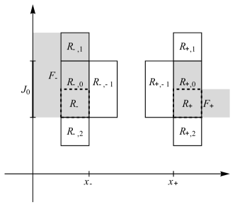
Figure 4: Map key for the notation in the proof of Lemma 5.

• by $J_{0}$ the maximal interval such that $\{x_{\pm}\}\times J_{0}\cap\partial R_{\pm}\neq\emptyset$ and $\{x_{\pm}\}\times J_{0}\subset\partial F_{\pm}$,

• by $R_{\pm,0}$ minimal rectangles in $\mathcal{F}(G)$ that have $\{x_{\pm}\}\times J_{0}$ as one of their sides and contained $R_{\pm}$,

• by $R_{+,-1}$ (resp. $R_{-,-1}$) the minimal rectangle in $\mathcal{F}(G)$ that has $\{x_{+}\}\times J_{0}$ (resp. $\{x_{-}\}\times J_{0}$) as one of its sides and does not contain $R_{+}$ (resp. $R_{-}$),

• by $K$ the number of endpoints of $J_{0}$ that do not intersect $\partial\Omega$ ($K\in\{0,1,2\})$,

• by $R_{\pm,j}$, $j\in\mathbb{N}$, $j\leq K$ the $K$ pairs of rectangles in $\mathcal{R}(G)$ such that

  • all of $R_{+,j}$, have a common side with $R_{+,0}$ and belong to the same column in $\mathcal{R}(G)$ as $R_{+}$,

  • all of $R_{-,j}$, have a common side with $R_{-,0}$ and belong to the same column in $\mathcal{R}(G)$ as $R_{-}$,

  • for a fixed $j$, both $R_{\pm,j}$ belong to the same row in $\mathcal{R}(G)$.

Due to the way these are defined, fixing $j\leq K$, at least one of the two rectangles $R_{\pm,j}$ is not contained in $F_{+}\cup F_{-}$, and

$$\text{at least one of inequalities }u|_{R_{+,j}}\!<\!u|_{R_{+,0}},\;u|_{R_{-,j}}\!>\!u|_{R_{-,0}}\text{ hold.}$$ (40)

If there is a pair of rectangles $R^{\prime}_{\pm}$ in $\mathcal{R}^{2}_{1,m}(G)$, $m<k$ such that $R^{\prime}_{\pm}\subset F_{\pm}$ then we have already proved that

$$\left|u|_{R_{+}}-u|_{R_{-}}\right|=\left|u|_{R^{\prime}_{+}}-u|_{R^{\prime}_{-}}\right|\leq\max_{(R_{1},R_{2})\in\mathcal{R}^{2}_{i,k}}\left|u_{0}|_{R_{1}}-u_{0}|_{R_{2}}\right|.$$

Therefore, we can assume that

$$u|_{R_{+,-1}}\!<\!u|_{R_{+,0}}\text{ and }u|_{R_{-,-1}}\!>\!u|_{R_{-,0}}\text{ hold.}$$ (41)

We have

$$F_{-}\in\mathrm{arg}\,\mathrm{min}\,\mathcal{J}_{F_{-},\partial F_{-}^{+},\partial F_{-}^{-},\frac{u_{0}}{\lambda}}\quad\text{and}\quad F_{+}\in\mathrm{arg}\,\mathrm{max}\,\check{\mathcal{J}}_{F_{+},\partial F_{+}^{+},\partial F_{+}^{-},\frac{u_{0}}{\lambda}}$$

(see the Remarks before the statement of Theorem 5 and after its proof). Therefore, taking into account (40, 41),

$$u|_{F_{+}}-u|_{F_{-}}=-\lambda\left(\check{\mathcal{J}}_{F_{+},\partial F_{+}^{+},\partial F_{+}^{-},\frac{u_{0}}{\lambda}}(F_{+})-\mathcal{J}_{F_{-},\partial F_{-}^{+},\partial F_{-}^{-},\frac{u_{0}}{\lambda}}(F_{-})\right)\\ \leq-\lambda\left(\check{\mathcal{J}}_{F_{+},\partial F_{+}^{+},\partial F_{+}^{-},\frac{u_{0}}{\lambda}}(R_{+})+\mathcal{J}_{F_{-},\partial F_{-}^{+},\partial F_{-}^{-},\frac{u_{0}}{\lambda}}(R_{-})\right)\\ \leq\frac{1}{\mathcal{L}^{2}(R_{+})}\int_{R_{+}}u_{0}\,\mathrm{d}\mathcal{L}^{2}-\frac{1}{\mathcal{L}^{2}(R_{-})}\int_{R_{-}}u_{0}\,\mathrm{d}\mathcal{L}^{2}\leq\max_{(R_{1},R_{2})\in\mathcal{R}^{2}_{i,k}}\left|u_{0}|_{R_{1}}-u_{0}|_{R_{2}}\right|.$$ (42)

∎

Theorem 8.

Let $\Omega$ be a rectangle and let $u$ be the solution to (4) with $u_{0}\in C(\Omega)$, $\lambda>0$. Then $u\in C(\Omega)$. In fact, if $\omega_{1},\omega_{2}\colon[0,\infty[\to[0,\infty[$ are continuous functions such that

$$|u_{0}(x_{1},x_{2})-u_{0}(y_{1},y_{2})|\leq\omega_{1}(|x_{1}-y_{1}|)+\omega_{2}(|x_{2}-y_{2}|)$$

for each $(x_{1},x_{2})$, $(y_{1},y_{2})$ in $\Omega$ then we have

$$|u(x_{1},x_{2})-u(y_{1},y_{2})|\leq\omega_{1}(|x_{1}-y_{1}|)+\omega_{2}(|x_{2}-y_{2}|)$$

for each $t>0$,$(x_{1},x_{2})$, $(y_{1},y_{2})$ in $\Omega$.

Remark.

Note that if $\omega$ is a concave modulus of continuity for $u_{0}$ with respect to norm $|\cdot|_{1}$, then $\omega_{1},\omega_{2}$ defined by $\omega_{1}=\omega_{2}=\omega$ satisfy the assumptions of Theorem 8. On the other hand, given $\omega_{1},\omega_{2}$ as in the Theorem, $\omega^{\prime}=\omega_{1}+\omega_{2}$ is a modulus of continuity for $u_{0}$ (as well as $u$). Theorem 8 implies for instance that if $L$ is the Lipschitz constant for $u_{0}$ with respect to norm $|\cdot|_{1}$, then the Lipschitz constant of $u$ with respect to norm $|\cdot|_{1}$ is not greater than $L$.

Proof.

We denote $\Omega=(s_{1},s_{2})+[0,l_{1}]\times[0,l_{2}]$. For $k=1,2,\ldots$ let

$$G_{k}=\left(\left\{s_{1}+\frac{jl_{1}}{k},j=0,1,\ldots,k\right\}\times\mathbb{R}\right)\cup\left(\mathbb{R}\times\left\{s_{2}+\frac{jl_{2}}{k},j=0,1,\ldots,k\right\}\right)$$

and let $u_{0,k}\in PCR(\Omega)$ be defined by

$$u_{0,k}(\boldsymbol{x})=u_{0}(\boldsymbol{x}_{R})\quad\text{for }\boldsymbol{x}\in R\in\mathcal{R}(G_{k}),$$

where $\boldsymbol{x}_{R}$ is the center of $R$.

For any $k=1,2,\ldots$, $i=1,2$, $m=0,\ldots,k-1$, let $(R,R^{\prime})\in\mathcal{R}^{2}_{i,m}(G_{k})$ with $(x_{1},x_{2})\in R,(y_{1},y_{2})\in R^{\prime}$ we have

$$\left|u_{0,k}|_{R}-u_{0,k}|_{R^{\prime}}\right|\leq\omega_{i}(|x_{i}-y_{i}|+\tfrac{1}{k}).$$ (43)

Let us denote by $u_{k}$ the solution to (4) with datum $u_{0,k}$. Due to inequality (43) and Lemma 5 we have for any $(x_{1},x_{2}),(y_{1},y_{2})\in\Omega$,

$$|u_{k}(x_{1},x_{2})-u_{k}(y_{1},y_{2})|\leq|u_{k}(x_{1},x_{2})-u_{k}(y_{1},x_{2})|+|u_{k}(y_{1},x_{2})-u_{k}(y_{1},y_{2})|\\ \leq\omega_{1}(|x_{1}-y_{1}|+\tfrac{1}{k})+\omega_{2}(|x_{2}-y_{2}|+\tfrac{1}{k}).$$

Now, due to monotonicity of $-\partial TV_{1,\Omega}$, we have $\|u_{k}-u\|_{L^{2}(\Omega)}\leq\|u_{0,k}-u_{0}\|_{L^{2}(\Omega)}.$ Therefore, there exists a set $N\subset\Omega$ of zero $\mathcal{L}^{2}$ measure and a subsequence $(k_{j})$ such that $u_{k_{j}}(\boldsymbol{x})\to u(\boldsymbol{x})\quad\text{for all }\boldsymbol{x}\in\Omega\setminus N.$ Now, for each pair $(x_{1},x_{2}),(y_{1},y_{2})\in\Omega$ take any pair of sequences $((x_{1,n},x_{2,n})),((y_{1,n},y_{2,n}))\subset\Omega\setminus N$ such that $x_{i,n}\to x_{i}$ and $y_{i,n}\to y_{i}$. Passing to the limit $j\to\infty$ and then $n\to\infty$ in

$$|u_{k_{j}}(x_{1,n},x_{2,n})-u_{k_{j}}(y_{1,n},y_{2,n})|\leq\omega_{1}(|x_{1,n}-y_{1,n}|+\tfrac{1}{k_{j}})+\omega_{2}(|x_{2,n}-y_{2,n}|+\tfrac{1}{k_{j}})$$

we conclude the proof. ∎

Analogous results can be obtained for the solutions to (5).

Lemma 6.

Let $\Omega$ be a rectangle, let $u$ be the solution to (5) with $u_{0}\in PCR(\Omega)$ and let $G$ be a grid such that $\mathcal{Q}_{u_{0}}$ is subordinate to $G$. Then for $i=1,2$ there holds

$$\max_{(R_{1},R_{2})\in\mathcal{R}^{2}_{i,m}(G)}\left|u(t,\cdot)|_{R_{1}}-u(t,\cdot)|_{R_{2}}\right|\leq\max_{(R_{1},R_{2})\in\mathcal{R}^{2}_{i,m}}\left|u_{0}|_{R_{1}}-u_{0}|_{R_{2}}\right|$$ (44)

in any time instance $t>0$.

Proof.

The form of solution obtained in Theorem 7 implies that the function

$$t\mapsto\max_{(R_{1},R_{2})\in\mathcal{R}^{2}_{i,m}(G)}\left|u(t,\cdot)|_{R_{1}}-u(t,\cdot)|_{R_{2}}\right|$$

is piecewise linear and continuous, in particular it does not have jumps. Having this observation in mind, let us consider time instance $\tau>0$ that does not belong to the set of merging times $\{t_{1},\ldots,t_{n}\}$.

For a given $0\leq k\leq m_{i}$ assume we have already proved that the slope of

$$t\mapsto\max_{(R_{1},R_{2})\in\mathcal{R}^{2}_{i,m}(G)}\left|u(t,\cdot)|_{R_{1}}-u(t,\cdot)|_{R_{2}}\right|$$

is non-positive in $t=\tau$ for each $0\leq m<k$. Take any pair of rectangles $(R_{+},R_{-})\in\mathcal{R}^{2}_{i,k}(G)$ that realizes the maximum in $\left|u(t,\cdot)|_{R_{1}}-u(t,\cdot)|_{R_{2}}\right|$. Let us take rectilinear polygons $F_{+},F_{-}$ in $\mathcal{Q}_{u(t,\cdot)}$ such that $R_{\pm}\subset F_{\pm}$.

Then, reasoning as in the proof of Lemma 5, we obtain

$$u_{t}(\tau,\cdot)|_{F_{+}}-u_{t}(\tau,\cdot)|_{F_{-}}=-\check{\mathcal{J}}_{F_{+},\partial F_{+}^{+},\partial F_{+}^{-}}(F_{+})+\mathcal{J}_{F_{-},\partial F_{-}^{+},\partial F_{-}^{-}}(F_{-})\\ \leq-\check{\mathcal{J}}_{F_{+},\partial F_{+}^{+},\partial F_{+}^{-}}(R_{+})+\mathcal{J}_{F_{-},\partial F_{-}^{+},\partial F_{-}^{-}}(R_{-})\leq 0$$ (45)

which concludes the proof. ∎

Now, note that if $u$ and $v$ are two solutions to (15) with $L^{2}(\Omega)$ initial data $u_{0}$ and $v_{0}$ respectively, we have for each time instance $t>0$ (see [28], Theorem 11.)

$$\|u(t,\cdot)-v(t,\cdot)\|_{L^{2}(\Omega)}\leq\|u_{0}-v_{0}\|_{L^{2}(\Omega)}.$$

Using this fact and Lemma 6, we can obtain the following analog of Theorem 8 for solutions of (15). The proof is almost identical and we omit it.

Theorem 9.

Let $\Omega$ be a rectangle and let $u$ be the solution to (15) with initial datum $u_{0}\in C(\Omega)$. Then $u(t,\cdot)\in C(\Omega)$ in every $t>0$. In fact, if $\omega_{1},\omega_{2}\colon[0,\infty[\to[0,\infty[$ are continuous functions such that

$$|u_{0}(x_{1},x_{2})-u_{0}(y_{1},y_{2})|\leq\omega_{1}(|x_{1}-y_{1}|)+\omega_{2}(|x_{2}-y_{2}|)$$

for each $(x_{1},x_{2})$, $(y_{1},y_{2})$ in $\Omega$ then we have

$$|u(t,(x_{1},x_{2}))-u(t,(y_{1},y_{2}))|\leq\omega_{1}(|x_{1}-y_{1}|)+\omega_{2}(|x_{2}-y_{2}|)$$

for each $t>0$,$(x_{1},x_{2})$, $(y_{1},y_{2})$ in $\Omega$.

Finally, we note that all the results in this section carry over in a straightforward way to the case $\Omega={\mathbb{R}^{2}}$, provided that in the statements of Theorems 8 and 9 $C(\Omega)$ is replaced with $C_{c,+}({\mathbb{R}^{2}})$ (meaning non-negative, compactly supported continuous functions on ${\mathbb{R}^{2}}$). On the other hand, if $\Omega$ is a rectilinear polygon different from a rectangle, the continuity is not necessarily preserved as Example 3 shows.

8 Examples

We start with the following general fact showing that minimizing (2) and solving (15) is equivalent in some cases.

Theorem 10.

Let $\Omega$ be a bounded domain or $\Omega={\mathbb{R}^{2}}$ and let $u$ be the strong solution to (15) in $[0,T[$ with initial datum $u_{0}\in L^{2}(\Omega)$. If there exists $\boldsymbol{z}\in L^{\infty}(]0,T[\times\Omega,{\mathbb{R}^{2}})$ satisfying conditions (16-19) such that for some $0<\lambda<T$ and almost all $0<t<\lambda$

$$\int_{\Omega}(\boldsymbol{z}(t,\cdot),Du(\lambda,\cdot))=\int_{\Omega}|Du(\lambda,\cdot)|_{\varphi}.$$ (46)

Then the minimizer of (2) with $\lambda>0$ is given by $u_{\lambda}=u(\lambda,\cdot)$.

Proof.

Let $\boldsymbol{z}_{\lambda}=\frac{1}{\lambda}\int_{0}^{\lambda}\boldsymbol{z}(t,\cdot)\,\mathrm{d}t$. Clearly, $\boldsymbol{z}_{\lambda}\in X_{\Omega}(u_{\lambda})$ satisfies $[\boldsymbol{z}_{\lambda},\boldsymbol{\nu}^{\Omega}]=0$ and $|\boldsymbol{z}_{\lambda}|^{*}_{\varphi}\leq 1$. Furthermore, by virtue of (46),

$$\int_{\Omega}(\boldsymbol{z}_{\lambda},Du_{\lambda})=\int_{\Omega}|Du_{\lambda}|_{\varphi},$$ (47)

so $\boldsymbol{z}_{\lambda}\in X_{\varphi,\Omega}(u_{\lambda})$. Finally, (16) implies

$$u_{\lambda}-u_{0}=\lambda\mathrm{div}\,\boldsymbol{z}_{\lambda}\quad\text{ in }\mathcal{D}^{\prime}(\Omega).$$ (48)

∎

One class of solutions to (15) such that (46) holds, are $PCR$ solutions constructed in Theorem (7) up to the first (positive) breaking time, as defined in the following

Definition 2.

Let $u\in W^{1,\infty}([0,\infty[,BV(\Omega))$ be the global strong solution to (5) with $u_{0}\in PCR(\Omega)$ and let $0<t_{1}<\ldots t_{n}$ be the sequence of time instances obtained in Theorem 7. We call each of $t_{1},\ldots,t_{n}$ a merging time. We say that $t_{i}$, $i=1,\ldots,n$ is a (positive) breaking time if $\mathcal{H}^{1}(J_{u(t,\cdot)}\setminus J_{u(t_{i},\cdot)})>0$ for $t\in]t_{i},t_{i+1}[$.

Indeed, let $t_{k}>0$ be the first breaking time and $0<t<\lambda\leq t_{k}$. Then $J_{u(\lambda,\cdot)}\subset J_{u(t,\cdot)}$ up to a $\mathcal{H}^{1}$-null set and $\frac{Du(\lambda,\cdot)}{|Du(\lambda,\cdot)|}=\frac{Du(t,\cdot)}{|Du(t,\cdot)|}$ holds $|Du(\lambda,\cdot)|$-a. e., which implies (46).

Now we provide several examples illustrating the strength of our results. Note that even though they are formulated in the language of the flow, in all of them $]0,\lambda[\ni t\mapsto\boldsymbol{z}(t,\boldsymbol{x})$ is constant a. e. for $|Du(\lambda,\cdot)|$-almost every $\boldsymbol{x}\in\Omega$ which implies (46), and therefore they are also solutions to (4).

Theorem 7 predicts that the jump set of a function piecewise constant on rectangles may expand under the $TV_{1}$ flow, i. e. facet breaking may occur. Many explicit examples of this kind can be constructed. Here we present a simple one, for which the procedure described in the proof of Theorem 6 is concise enough to be presented in detail.

Example 1.

Let

$$u(t,\cdot)=\left(1-\tfrac{4}{3}t\right)_{+}\chi_{B}+\left(1-2t\right)_{+}\chi_{C},$$

where we denoted

$$B=B_{\infty}\left((0,0),\tfrac{3}{2}\right),\quad C=B_{\infty}\left((2,0),\tfrac{1}{2}\right)\cup B_{\infty}\left((-2,0),\tfrac{1}{2}\right)\cup B_{\infty}\left((0,2),\tfrac{1}{2}\right)\cup B_{\infty}\left((0,-2),\tfrac{1}{2}\right).$$

For each $t\geq 0$, $u(t,\cdot)\in PCR_{+}({\mathbb{R}^{2}})$ and $u$ solves (5) with initial datum $u_{0}=\chi_{B\cup C}$. To see this, we execute the algorithm described in Theorem 6. Let $Q_{1}=u_{0}^{-1}(1)=B\cup C$. Due to symmetry, the only plausible largest minimizers of $\mathcal{J}_{Q_{1},\partial Q_{1},\emptyset,0}$ are $B$, $C$ and $B\cup C$ (we only need to consider elements of $\mathcal{F}_{u_{0}}$ and no subset of square $B$ can produce lower value of the functional than $B$). We check that the values of $\mathcal{J}_{Q_{1},\partial Q_{1},\emptyset,0}$ on these sets are, respectively, $\frac{4}{3}$, $4$, and $\frac{20}{13}$, hence $B$ is the minimizer and the initial velocity on $B$ is $-\frac{4}{3}$. Next, we have to find the largest minimizer of $\mathcal{J}_{C,\partial Q_{1},\partial B,0}$. There is only one competitor, $C$. To find initial velocity on $C$, we calculate $-\mathcal{J}_{C,\partial Q_{1},\partial B,0}(C)=-2$. Finally, as explained in section 6, we need to find the largest minimizer of $\mathcal{J}_{Q_{0},\partial R_{0},\partial Q_{1},0}$, where we denoted $R_{0}$ to be the smallest rectangle (square) containing the support of $u_{0}$ and $Q_{0}=R_{0}\cap u_{0}^{-1}(0)$. We check that the minimizer is $Q_{0}$ itself, with $\mathcal{J}_{Q_{0},\partial R_{0},\partial Q_{1},0}(Q_{0})=0$.

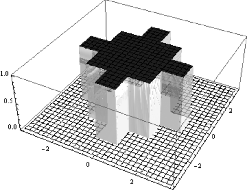
(a) $t=0$.

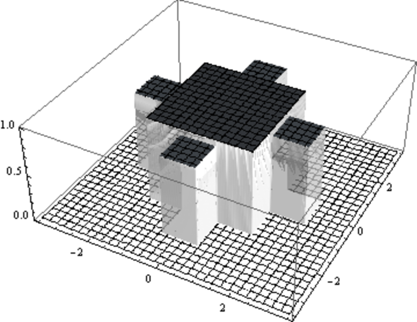
(b) $t=0.08$.

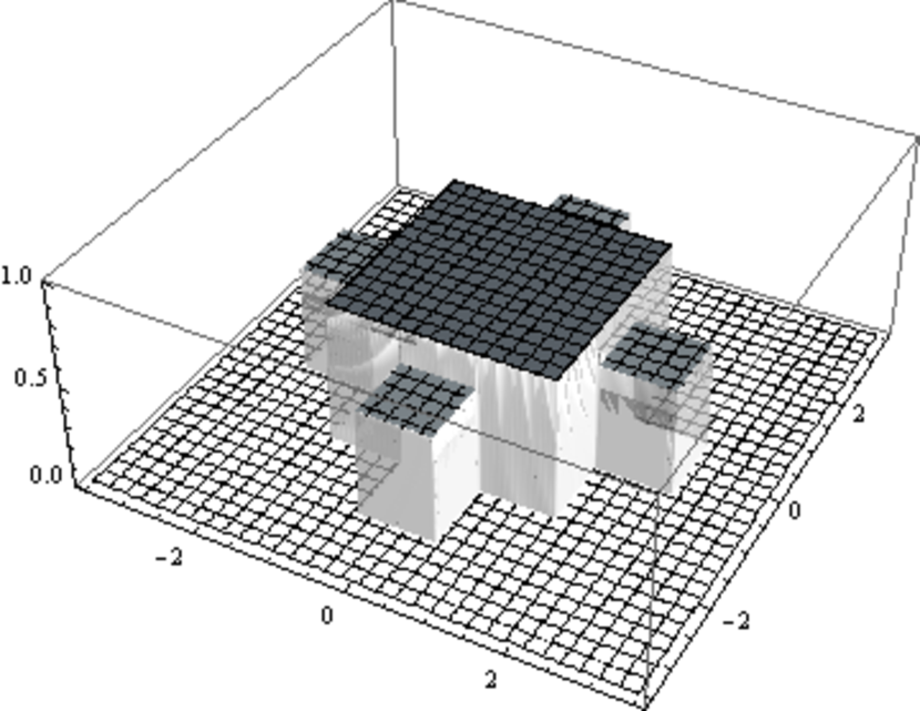
(c) $t=0.24$.

Figure 5: Plots of $u(t,\cdot)$ from Example 1 in certain time instances $t$.

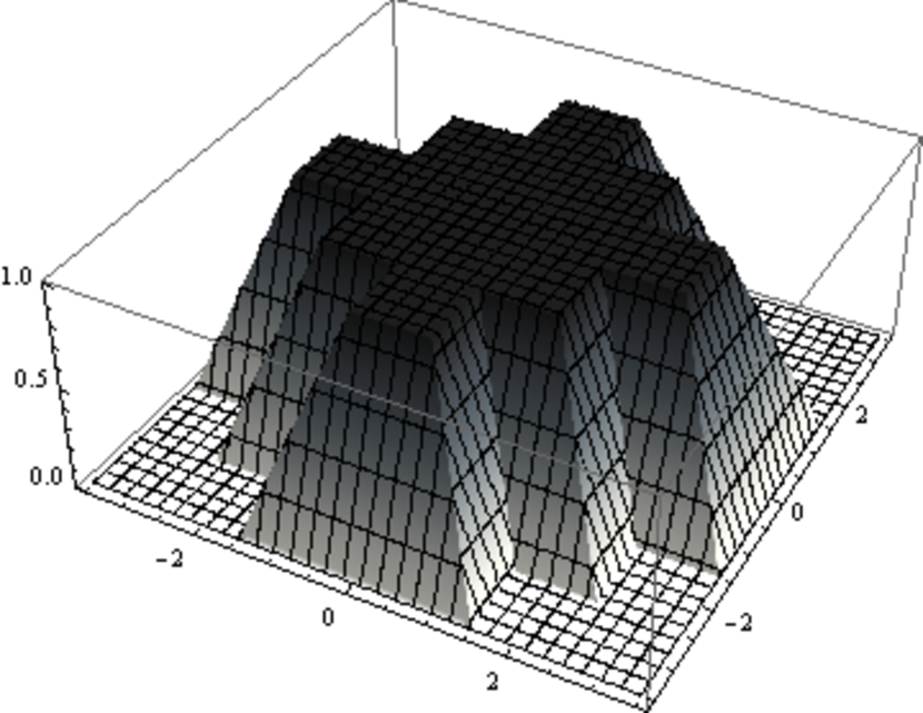
(a) $t=0$.

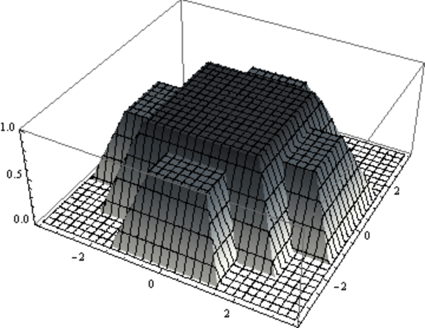
(b) $t=0.08$.

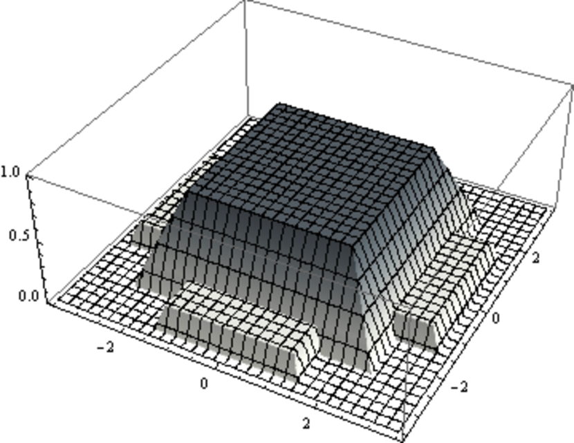
(c) $t=0.24$.

Figure 6: Plots of $u(t,\cdot)$ from Example 2 in certain time instances $t$.

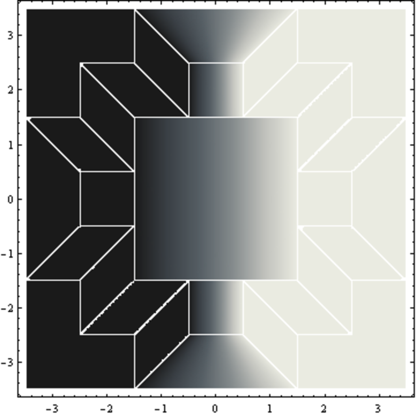
(a) $t=0$.

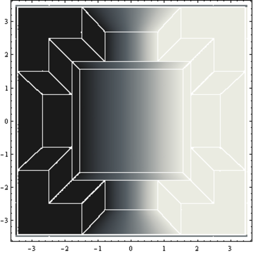
(b) $t=0.08$.

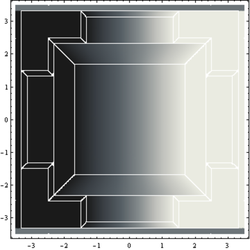
(c) $t=0.24$.

Figure 7: Density plots of $z_{1}(t,\cdot)$ corresponding to $u(t,\cdot)$ from Example 2 in certain time instances $t$. Black corresponds to value $1$, ivory to $-1$; note the value $0$ outside the minimal strip containing the support of $u(t,\cdot)$.

On the other hand, Theorem 8 asserts that if $u_{0}$ is (Lipschitz) continuous, the solution $u$ starting with $u_{0}$ is (Lipschitz) continuous in every time instance $t>0$. For instance, if one extends the characteristic function form Example 1 continuously outside its support, no jumps will appear in the evolution — another manifestation of nonlocality of the equation.

Example 2.

Here we present Figure 6, depicting evolution $u$ of piecewise linear continuous function $u_{0}$ obtained by extending the initial datum from Example 1 outside its support up to $0$ in such a way that $\nabla u_{0}\in\{(0,0),(1,0),(0,1)\}$. The evolution is obtained by explicit identification of corresponding field $\boldsymbol{z}=(z_{1},z_{2})$ under an ansatz that in each of a finite number of evolving regions either $z_{i}=\pm 1$ or a $z_{i}$ is a linear interpolation of boundary values, $i=1,2$ (see Figure 7). This reduces the problem to a decoupled infinite system of ODEs. The evolution obtained this way is the strong solution starting with $u_{0}$ as it satisfies all the requirements in Definition 1. Figures 6 and 7 are obtained by solving numerically the system of ODEs using Mathematica’s NDSolve function. We omit the quite lengthy details.

Next we provide an example showing that in non-convex rectilinear polygons (i. e. other than a rectangle) evolution starting with continuous initial datum may develop discontinuities.

Example 3.

Let

$$\Omega=\{(x_{1},x_{2})\colon|(x_{1},x_{2})|_{\infty}\leq 1,x_{1}\leq 0,x_{2}\leq 0\},\quad u_{0}(x_{1},x_{2})=x_{2}$$

and so $\nabla u(0,\cdot)\equiv(0,1)$, $\boldsymbol{z}(0,\cdot)\equiv(0,1)$. The solution can be written explicitly, for $t\leq\frac{1}{8}$ we have

$$u(t,x_{1},x_{2})=\left\{\begin{array}[]{ll}-1+\sqrt{2t}&\text{if }x_{2}\leq-1+\sqrt{2t},\\ -\sqrt{2t}&\text{if }x_{1}\geq 0\text{ and }x_{2}\geq-\sqrt{2t},\\ 1-\sqrt{2t}&\text{if }x_{1}<0\text{ and }x_{2}\geq 1-\sqrt{2t},\\ x_{2}&\text{otherwise.}\end{array}\right.$$

We see that regions where $\nabla u=0$ appear near the boundary and expand with speed $\frac{1}{\sqrt{2t}}$. In these regions, $z_{2}$ is a linear interpolation between $0$ and $1$. Also a jump in the $x_{2}$ direction appears near $\boldsymbol{x}=0$ and grows with the same speed.

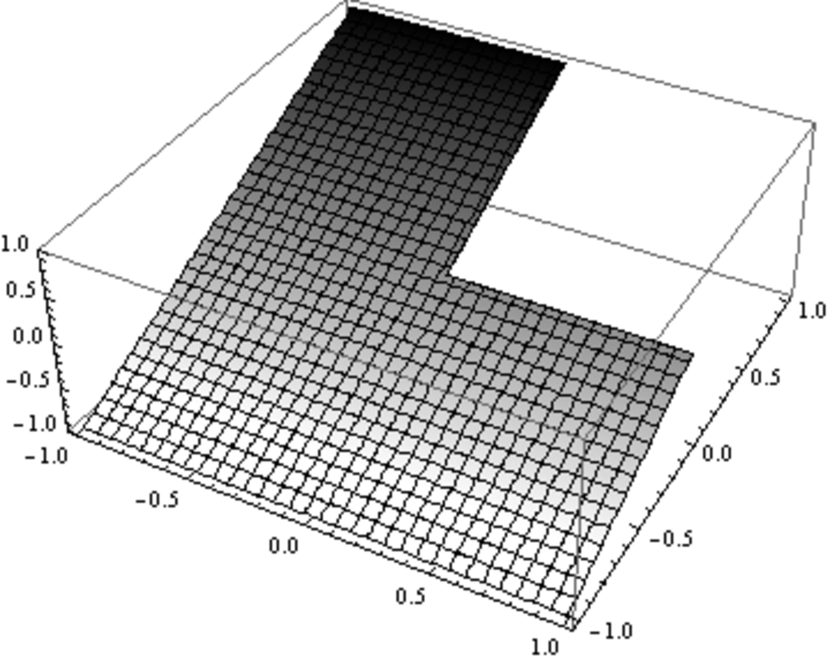
(a) $t=0$.

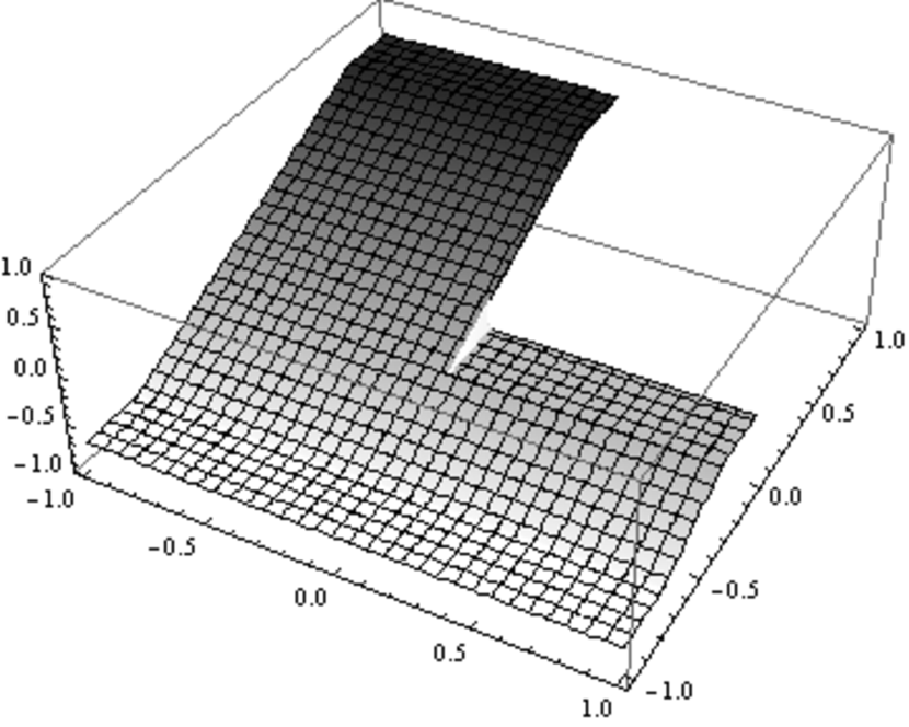
(b) $t=0.04$.

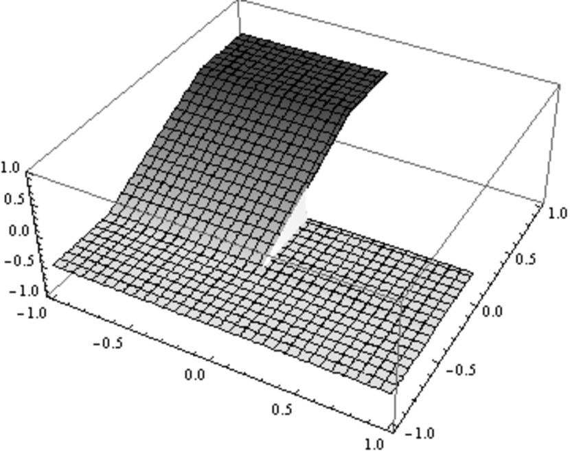
(c) $t=0.12$.

Figure 8: Plots of $u(t,\cdot)$ from Example 3 at certain time instances $t$.

Finally, let us present exact calculation for an example of the phenomenon of bending, which shows effectiveness of approximation with $PCR$ functions.

Example 4.

Let $\Omega={\mathbb{R}^{2}}$, $u_{0}=\chi_{B_{1}(2)}$. We will show that the solution to (5) is given by

$$u(t,\boldsymbol{x})=(1-v(\boldsymbol{x})t)_{+},$$

with $v=\frac{1}{2-\sqrt{2}}\chi_{B_{\infty}(\sqrt{2})\cap B_{1}(2)}+\frac{1}{2-|\boldsymbol{x}|_{\infty}}\chi_{B_{1}(2)\setminus B_{\infty}(\sqrt{2})}$.

In order to prove the claim, we approximate $B_{1}(2)$ by a family of rectilinear polygons as follows. Given $n\in\mathbb{N}$, we define inductively

$$\left\{\begin{array}[]{l}A_{1,1}:=B_{\infty}(1)\\ A_{k,1}:=B_{\infty}((\frac{2(k-1)}{n},0),1-\frac{k-1}{n})\setminus A_{k-1,1}{\rm\ \ for\ }k=2,\ldots,n\end{array}\right..$$

We observe that $\bigcup_{k=1}^{n}A_{k,1}$ is an increasing sequence with respect to $n$ and that

$$\lim_{n\to\infty}\bigcup_{k=1}^{n}A_{k,1}=B_{1}(2)\cap\{x_{1}>0,-1\leq x_{2}\leq 1\}.$$

By symmetry, we construct $A_{k,2}$, $A_{k,3}$ and $A_{k,4}$ for $k=1,\ldots,n$ such that

$$\lim_{n\to\infty}\bigcup_{k=1}^{n}A_{k,2}=B_{1}(2)\cap\{x_{2}>0,-1\leq x_{1}\leq 1\},$$

$$\lim_{n\to\infty}\bigcup_{k=1}^{n}A_{k,3}=B_{1}(2)\cap\{x_{1}<0,-1\leq x_{2}\leq 1\},$$

$$\lim_{n\to\infty}\bigcup_{k=1}^{n}A_{k,4}=B_{1}(2)\cap\{x_{2}<0,-1\leq x_{1}\leq 1\}.$$

Therefore, $B_{1}(2)=\lim_{n\to\infty}A_{n}:=\bigcup_{k=1}^{n}\bigcup_{j=1}^{4}A_{k,j}.$

We let $C_{k}:=\bigcup_{j=1}^{4}A_{k,1}$, for $k=1,\ldots,n$. Observe that the inequality

$$\frac{{\rm Per}_{1}(C_{1}\cup\ldots\cup C_{k+1})}{|C_{1}\cup\ldots\cup C_{k+1})|}>\frac{{\rm Per}_{1}(C_{1}\cup\ldots\cup C_{k})}{|C_{1}\cup\ldots\cup C_{k})|}$$

holds (and therefore the facet $C_{k+1}$ breaks from $C_{1}\cup\ldots\cup C_{k})$ iff

$$\frac{1}{1-\frac{k}{n}}>\frac{{\rm Per}_{1}(C_{1}\cup\ldots\cup C_{k})}{|C_{1}\cup\ldots\cup C_{k})|}=2\frac{1+\frac{k-1}{n}}{1+\frac{2(k-1)}{n}(1-\frac{k}{2n})}\leftrightarrow\frac{k}{n}\geq\sqrt{\left(1-\frac{1}{2n}\right)^{2}+1}-\left(1-\frac{1}{2n}\right).$$

Since the speed of $C_{j}$ is given by $\frac{1}{1-\frac{j}{n}}$ (which increases with respect to $j=k+1,\ldots,n$), once $C_{k+1}$ breaks from $C_{1}\cup\ldots\cup C_{k})$, so do $C_{j}$ from $C_{j-1}$ for $j=k+1,\ldots,n$. Therefore, the solution for $u_{0,n}=\chi_{A_{n}}$ is given by

$$u_{n}(t,\boldsymbol{x})=\left(1-\frac{{\rm Per}_{1}(C_{1}\cup\ldots\cup C_{k})}{|C_{1}\cup\ldots\cup C_{k})|}t\right)_{+}\chi_{(C_{1}\cup\ldots\cup C_{k})}+\sum_{j=k+1}^{n}\left(1-\frac{1}{1-\frac{j}{n}}t\right)_{+}\chi_{C_{j}},$$ (49)

with $k\in\mathbb{N}$ satisfying

$$[k-1]<n\left(\sqrt{\left(1-\frac{1}{2n}\right)^{2}+1}-\left(1-\frac{1}{2n}\right)\right)\leq[k].$$

Letting $n\to\infty$ in (49), we finish the proof.

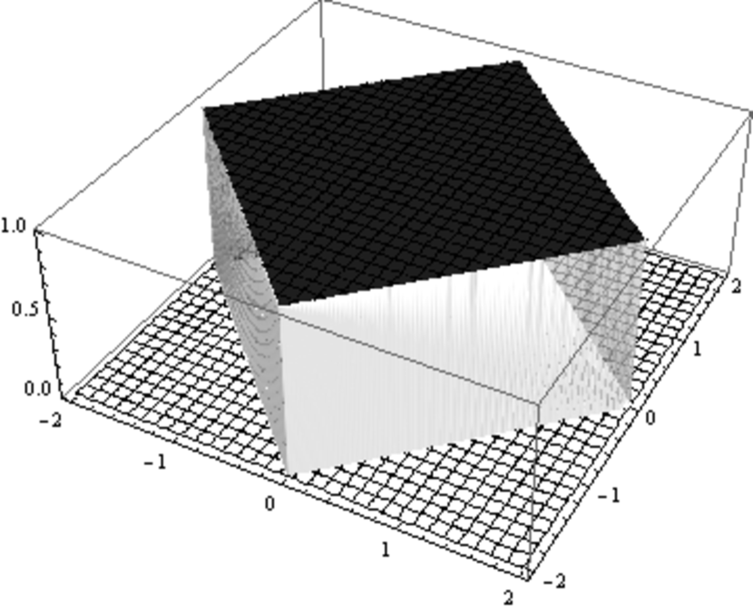
(a) $t=0$.

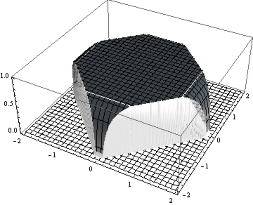
(b) $t=0.1$.

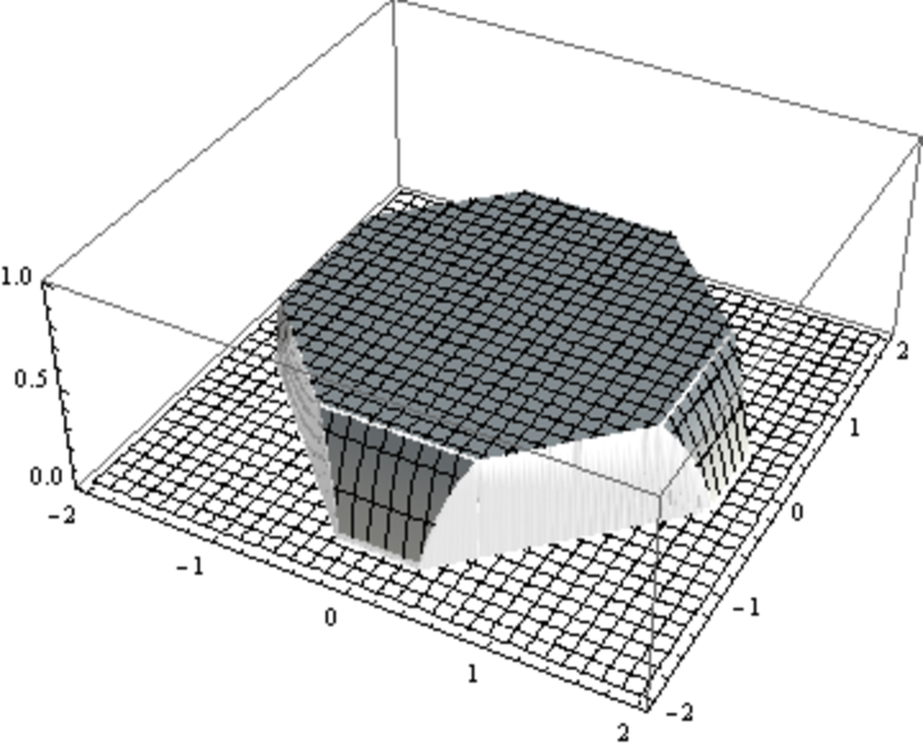
(c) $t=0.3$.

Figure 9: Plots of $u(t,\cdot)$ from Example 4 at certain time instances $t$.

The evolution of a bounded convex domain $C$ satisfying an interior ball condition was explicitly given in [13, Section 8.3]. There, the authors defined a notion of anisotropic variational mean curvature, denoted by $H_{C}\colon\mathbb{R}^{N}\to]-\infty,0]$, based on the solvability of some auxiliary minimizing problems and on the existence of a Cheeger set in $C$. Then, the solution to (15) with data $u_{0}=\chi_{C}$ was given by

$$u(t,\boldsymbol{x})=(1+H_{C}(\boldsymbol{x})t)_{+}\chi_{C}(\boldsymbol{x}).$$

In general, it is not obvious how to compute this anisotropic variational mean curvature. However, Example 4 shows that one can compute it by approximation of the set $C$ with rectilinear polygons, even in the case that $C$ does not satisfy the interior ball condition. Note that the solution starting with initial datum as in Example 4 was calculated with an approximate numerical procedure in [29]. Here, we provided the exact evolution in this case.

9 Conclusions

The core of our results is the explicit construction of tetris-like solutions, i. e. solutions in the $PCR$ class. This class can be viewed as a natural generalization of mono-dimensional step functions, whose finite dimensional structure allows to effectively reduce the original nonlinear problem. The directional diffusion allows to analyze the solutions only in a grid given by a suitably chosen initial datum. We treat them as generic objects in the set of all weak solutions, hence $PCR$ solutions are indeed smooth functions in the new analytical language exclusively dedicated to our variational problem. The detailed prescription of solutions allows to prove even conservation of moduli of continuity for continuous initial data. It, unexpected, removes this classical viewpoint on the issue of solvability out of our interests. Just information obtained for $PCR$ functions is much more complete than any knowledge of regularity in the classical setting.

At the end we would like to say a few words about the weakness of the approach. The procedure works due to the possibility of introducing a grid. It is the consequence of symmetry given by the $|\cdot|_{1}$ norm, the grid is just determined by directions $\hat{e}_{x_{1}}$, $\hat{e}_{x_{2}}$ for the initial datum. Here we have a natural shift symmetry, and the same structure at each vertex of the grid. It seems that it would be possible to attempt to repeat at least some of our analysis for anisotropic norms that generate a tiling of the plane. Here we think of $|\cdot|_{\phi}$ determined by the hexagon, and tiling given by honeycomb structure. We are highly limited by regular tiling (triangular, rectangular and hexagonal), however it seems to be possible to introduce more complex structure for different anisotropy. Such problems will definitely require new framework not linked to the classical analysis.

References

- [1] M. Amar and G. Bellettini, A notion of total variation depending on a metric with discontinuous coefficients, Ann. Inst. H. Poincaré Anal. Non Linéaire, 11 (1994), pp. 91–133.
- [2] L. Ambrosio, N. Fusco, and D. Pallara, Functions of bounded variation and free discontinuity problems, Oxford Mathematical Monographs, The Clarendon Press, Oxford University Press, New York, 2000.
- [3] G. Anzellotti, Pairings between measures and bounded functions and compensated compactness, Ann. Mat. Pura Appl. (4), 135 (1983), pp. 293–318 (1984), doi:10.1007/BF01781073.
- [4] V. Barbu, Nonlinear differential equations of monotone types in Banach spaces, Springer Monographs in Mathematics, Springer, New York, 2010, doi:10.1007/978-1-4419-5542-5.
- [5] G. Bellettini, V. Caselles, and M. Novaga, The total variation flow in , J. Differential Equations, 184 (2002), pp. 475–525, doi:10.1006/jdeq.2001.4150.
- [6] G. Bellettini, M. Novaga, and M. Paolini, On a crystalline variational problem. I. First variation and global regularity, Arch. Ration. Mech. Anal., 157 (2001), pp. 165–191, doi:10.1007/s002050010127.
- [7] G. Bellettini, M. Novaga, and M. Paolini, On a crystalline variational problem. II. regularity and structure of minimizers on facets, Arch. Ration. Mech. Anal., 157 (2001), pp. 193–217, doi:10.1007/s002050100126.
- [8] B. Berkels, M. Burger, M. Droske, O. Nemitz, and M. Rumpf, Cartoon extraction based on anisotropic image classification vision, modeling, and visualization, in Vision, Modeling, and Visualization 2006: Proceedings, November 22-24, 2006, Aachen, Germany, IOS Press, 2006, p. 293.
- [9] M. Bonforte and A. Figalli, Total variation flow and sign fast diffusion in one dimension, J. Differential Equations, 252 (2012), pp. 4455–4480, doi:10.1016/j.jde.2012.01.003.
- [10] A. Briani, A. Chambolle, M. Novaga, and G. Orlandi, On the gradient flow of a one-homogeneous functional, Confluentes Math., 3 (2011), pp. 617–635, doi:10.1142/S1793744211000461.
- [11] M. Burger, G. Gilboa, M. Moeller, L. Eckardt, and D. Cremers, Spectral decompositions using one-homogeneous functionals, SIAM J. Imaging Sci., 9 (2016), pp. 1374–1408, doi:10.1137/15M1054687.
- [12] E. Casas, K. Kunisch, and C. Pola, Regularization by functions of bounded variation and applications to image enhancement, Appl. Math. Optim., 40 (1999), pp. 229–257, doi:10.1007/s002459900124.
- [13] V. Caselles, A. Chambolle, S. Moll, and M. Novaga, A characterization of convex calibrable sets in with respect to anisotropic norms, Ann. Inst. H. Poincaré Anal. Non Linéaire, 25 (2008), pp. 803–832, doi:10.1016/j.anihpc.2008.04.003.
- [14] V. Caselles, A. Chambolle, and M. Novaga, The discontinuity set of solutions of the TV denoising problem and some extensions, Multiscale Model. Simul., 6 (2007), pp. 879–894, doi:10.1137/070683003.
- [15] V. Caselles, A. Chambolle, and M. Novaga, Regularity for solutions of the total variation denoising problem, Rev. Mat. Iberoam., 27 (2011), pp. 233–252, doi:10.4171/RMI/634.
- [16] A. Chambolle and J. Darbon, On total variation minimization and surface evolution using parametric maximum flows, Numer. Math. Theory Methods Appl., 84 (2009).
- [17] R. H. Chan, S. Setzer, and G. Steidl, Inpainting by flexible Haar-wavelet shrinkage, SIAM J. Imaging Sci., 1 (2008), pp. 273–293, doi:10.1137/070711499.
- [18] H. Chen, C. Wang, Y. Song, and Z. Li, Split Bregmanized anisotropic total variation model for image deblurring, J. Vis. Comun. Image Represent., 31 (2015), pp. 282–293, doi:10.1016/j.jvcir.2015.07.004.
- [19] R. Choksi, Y. van Gennip, and A. Oberman, Anisotropic total variation regularized approximation and denoising/deblurring of 2D bar codes, Inverse Probl. Imaging, 5 (2011), pp. 591–617, doi:10.3934/ipi.2011.5.591.
- [20] S. Esedoḡlu and S. J. Osher, Decomposition of images by the anisotropic Rudin-Osher-Fatemi model, Comm. Pure Appl. Math., 57 (2004), pp. 1609–1626, doi:10.1002/cpa.20045.
- [21] B. G. Fitzpatrick and S. L. Keeling, On approximation in total variation penalization for image reconstruction and inverse problems, Numer. Funct. Anal. Optim., 18 (1997), pp. 941–958, doi:10.1080/01630569708816802.
- [22] E. Giusti, Minimal surfaces and functions of bounded variation, vol. 80 of Monographs in Mathematics, Birkhäuser Verlag, Basel, 1984, doi:10.1007/978-1-4684-9486-0.
- [23] T. Goldstein and S. Osher, The split Bregman method for -regularized problems, SIAM J. Imaging Sci., 2 (2009), pp. 323–343, doi:10.1137/080725891.
- [24] M. Grasmair and F. Lenzen, Anisotropic total variation filtering, Appl. Math. Optim., 62 (2010), pp. 323–339, doi:10.1007/s00245-010-9105-x.
- [25] D. S. Hochbaum, Multi-label Markov random fields as an efficient and effective tool for image segmentation, total variations and regularization, Numer. Math. Theory Methods Appl., 6 (2013), pp. 169–198.
- [26] K. Kielak, P. B. Mucha, and P. Rybka, Almost classical solutions to the total variation flow, J. Evol. Equ., 13 (2013), pp. 21–49, doi:10.1007/s00028-012-0167-x.
- [27] G. Mercier, Continuity results for TV-minimizers, Preprint, arXiv:1605.09655, (2016).
- [28] S. Moll, The anisotropic total variation flow, Math. Ann., 332 (2005), pp. 177–218, doi:10.1007/s00208-004-0624-0.
- [29] P. B. Mucha, M. Muszkieta, and P. Rybka, Two cases of squares evolving by anisotropic diffusion, Adv. Differential Equations, 20 (2015), pp. 773–800.
- [30] W. Ring, Structural properties of solutions to total variation regularization problems, ESAIM: Mathematical Modelling and Numerical Analysis, 34 (2000), pp. 799–810.
- [31] L. I. Rudin, S. Osher, and E. Fatemi, Nonlinear total variation based noise removal algorithms, Phys. D, 60 (1992), pp. 259–268. Experimental mathematics: computational issues in nonlinear science (Los Alamos, NM, 1991).
- [32] S. Setzer, G. Steidl, and T. Teuber, Restoration of images with rotated shapes, Numer. Algorithms, 48 (2008), pp. 49–66, doi:10.1007/s11075-008-9182-y.