Central loops in random planar graphs

Abstract

Random planar graphs appear in a variety of context and it is important for many different applications to be able to characterize their structure. Local quantities fail to give interesting information and it seems that path-related measures are able to convey relevant information about the organization of these structures. In particular, nodes with a large betweenness centrality (BC) display non-trivial patterns, such as central loops. We first discuss empirical results for different random planar graphs and we then propose a toy model which allows us to discuss the condition for the emergence of non-trivial patterns such as central loops. This toy model is made of a star network with $N_{b}$ branches of size $n$ and links of weight $1$, superimposed to a loop at distance $\ell$ from the center and with links of weight $w$. We estimate for this model the BC at the center and on the loop and we show that the loop can be more central than the origin if $w<w_{c}$ where the threshold of this transition scales as $w_{c}\sim n/N_{b}$. In this regime, there is an optimal position of the loop that scales as $\ell_{opt}\sim N_{b}w/4$. This simple model sheds some light on the organization of these random structures and allows us to discuss the effect of randomness on the centrality of loops. In particular, it suggests that the number and the spatial extension of radial branches are the crucial ingredients that control the existence of central loops.

I Introduction

Random planar graphs – random graphs that can be drawn on the 2d plane with no edge crossing Clark:1991 – pervade many different fields from abstract mathematics Tutte:1963 ; Bouttier:2004 , to theoretical physics Ambjorn:1997 , botanics Weitz:2012 ; Katifori:2012 , geography and urban studies Barthelemy:2011 . In particular, planar graphs are central in biology where they can be used to describe veination patterns of leaves or insect wings and which display an interesting architecture with many loops at different scales Weitz:2012 ; Katifori:2012 ; Katifori:2010 ; Hu:2013 . In the study of urban systems, planar networks are extensively used to represent, to a good approximation, various infrastructure networks Barthelemy:2011 such as transportation networks Haggett:1969 and streets patterns Hillier:1984 ; Marshall:2006 ; Jiang:2004 ; Roswall:2005 ; Porta:2006 ; Porta:2006b ; Lammer:2006 ; Crucitti:2006 ; Cardillo:2006 ; Xie:2007 ; Jiang:2007 ; Masucci:2009 ; Chan:2011 ; Courtat:2011 ; Strano:2012 ; Barthelemy:2013 ; Viana:2013 ; Louf:2014 ; Porta:2014 . Understanding the structure and the evolution of these networks is therefore interesting from a purely graph theoretical point of view, but could also have an impact in different fields where these structures are central.

Most previous studies characterize different aspects of these graphs, either purely topological (degree distribution, clustering, etc.) or geometrical (angles, segment length, face area distribution, etc.). Due to spatial constraints, most local information such as the degree distribution, the clustering or the assortativity have however a trivial behavior Barthelemy:2011 . In addition the important information about these random planar graphs is in fact not in their adjacency matrix only but also in their geometry described by the spatial distribution of nodes and relevant meaures should combine topology and geometry. Despite the large number of studies on these graphs, there is still a lack of a non-local high-level metrics that allow for understanding and comparing these graphs with each other. However, a promising direction is given by path-based quantities such as the simplicity Aldous:2010 ; Viana:2013 or as we will discuss here, the betweenness centrality (BC) Freeman:1977 . The BC was introduced to quantify the importance of a node (or an edge) in a network, but it also proved to be a very interesting tool in the study of random planar graphs. Already in Lammer:2006 , interesting spatial patterns of nodes with large BC were observed. More recently, it has been shown that the most salient aspects of the structural changes during the evolution of the street network of Paris Barthelemy:2013 is revealed by the spatial distribution of the nodes with the largest BC. These different results therefore point to the fact that high centrality nodes form non-trivial patterns, and among them, the emergence of loops. All these different results point to the fact the BC, which is relatively simple, is a good candidate for monitoring and understanding the organization of random planar graphs. In this study we will focus on the apearance of loops made of links with large BC and we will propose a simple toy model that allows us to discuss the conditions for the appearance of such patterns.

The emergence of rings in largely urbanized areas is a common fact and the study presented here gives a topological light on this phenomenon. Our study echoes previous work where congestion effect at a central hub could be so high that avoiding the ring is beneficial Ashton:2005 ; Jarrett:2006 . Here, in contrast, we do not take into account congestion and discuss the conditions necessary for a loop to become more interesting in terms of time cost.

II The BC for planar graphs

Basic results on planar networks can be found in any graph theory textbook (see for example Clark:1991 and for useful algorithms see Jungnickel:2008 ) and we will very briefly recall the definition of these objects. Basically, a planar graph is a graph that can be drawn in the plane in such a way that its edges do not intersect. Not all drawings of planar graphs are without intersection and a drawing without intersection is sometimes called a plane graph or a planar embedding of the graph. In real-world cases, these considerations actually do not apply since the nodes and the edges represent in general physical objects. More precisely, we will focus here on the case of planar graphs embedded in 2d space, which typically describes systems such as the road and street network.

II.1 Definition of the BC and variants

The betweenness centrality counts the fraction of shortest paths going through a given node (or link) and is given by Freeman:1977

$$g(v)={\cal N}\sum_{s\neq t}\frac{\sigma_{st}(v)}{\sigma_{st}}$$ (1)

where $v$ is a node, $\sigma_{st}$ is the number of shortest paths from $s$ to $t$ and $\sigma_{st}(v)$ those paths going through $v$. In general the summation is on $s\neq t$ and $s\neq v$, $t\neq v$ and this is the convention that we will adopt in this paper. The constant ${\cal N}$ is the normalisation and we will use here ${\cal N}=1/(N-1)(N-2)$ which counts the number of pairs and ensures that $g(v)\in[0,1]$. For edges, the definition of the BC is similar to Eq. 1.

It is important to stress here that the BC could in fact be defined for any type of paths. The most common choice is the shortest path but we will use the more general case of weighted shortest path, which corresponds to the quickest path if the weight of a link represents time. For numerical calculations, we implemented the now standard algorithm of Brandes Brandes:2001 .

II.2 Regular lattice

In a one-dimensional lattice of size $n$, the BC of a site $0\leq x\leq n$ is given by

$$g(x)=x(n-x)$$ (2)

and the maximum thus corresponds to the barycenter of all nodes (see Fig.1) (in the two-dimensional case we obtain a similar behavior).

Figure 1: Betweenness centrality for a one-dimensional lattice. (Left) When there is no disorder, the barycenter is the most central nodes. (Right) In the case of a disordered network, degree becomes relevant and the most central nodes have large degrees.

When we introduce disorder - by removing or rewiring links - the BC becomes important at nodes that can be far away from the barycenter (see Fig.1). In the extreme case where space doesn’t play a role anymore such as in scale-free networks, the average BC per degree classes $g(k)$ scales as Barthelemy:2004

$$g(k)\sim k^{\eta}$$ (3)

where $\eta$ is an exponent that depends on the structure of the graph. Even if there are fluctuations around this scaling it shows here that essentially the degree controls the BC in these graphs.

II.3 Percolation: giant component

A simple way to construct a random planar graph is to consider a regular lattice where each link has a probabilty $f$ to be removed (and $p=1-f$ to be present). Above the percolation threshold ($p\geq p_{c}$), the system displays a giant component which connects a non-zero fraction of the nodes. We can study the BC on this giant component and filter them for different threshold $g^{*}$: we keep only links with centrality $g$ such that $g>g^{*}$. We show in Fig. 2 the set of links that belong to the giant component and with BC larger than $g^{*}$ and represent the BC with a color code (from dark blue to yellow).

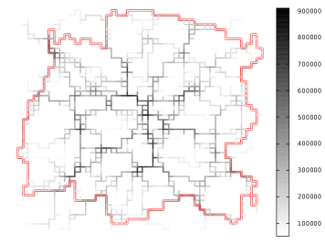
Figure 2: Links belonging to the giant component obtained for percolation with $f=0.15$ and with normalized BC larger than $g^{*}=0.05g_{max}$. We observe that the links with a very large BC form a non-trivial pattern and are not necessarily close to the center. The largest loop is here highlighted with a double line.

and we observe that the set of most central links forms a non-trivial pattern where the distance to the center is not the main determinant (Fig. 2). In particular, we observe the presence of very central links that are not close to the center and that depend on the particular disorder configuration.

We can go further in the analysis of the structure of the percolating cluster by analyzing the ratio

$$\eta=\frac{g(r,\theta)}{\max_{r^{\prime}<r,\theta^{\prime}\in[0,2\pi]}g(r,\theta^{\prime})}$$ (4)

which compares the BC at one point with the maximum BC of nodes in the region closer to the origin. For a percolating cluster obtained at $p=0.8$ (well above the percolation threshold) and on a lattice $100\times 100$, we observe a very broad distribution of $\eta$. For values larger than one we obtain on average $\overline{\eta}\simeq 3$ and a very large dispersion of order $10^{3}$. We can observe the points for which we have a ratio $\eta>1$ and plot (Fig. 3) the distribution of the distance to the center for these points (normalized by the maximum distance $d_{max}$).

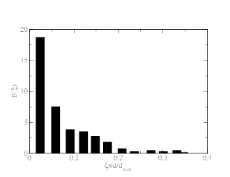
Figure 3: Distribution of the distance (normalized by the maximum distance on the lattice) to the center for nodes with a ratio $\eta>1$. These results were obtained for $p=0.8$ on a $100\times 100$ lattice and averaged over $30$ configurations.

This figure 3 shows that the location of nodes with a very large BC (at least larger than the BC of the nodes closer to the center) can be of order the system size. This shows that – depending on the disorder – the ‘central’ area composed of the geometrical center and its surroundings are composed of nodes with a relatively small BC. This reinforces the need to understand in which cases the monotoneous decrease of the BC with the distance to center can be strongly modified by fluctuations.

II.4 Real-world planar graphs

Streets and roads form a network where nodes are intersections and links are segment roads, and which is planar (or almost planar, to a good approximation). This network is now fairly well characterized and due to spatial constraints, the degree distribution is peaked, the clustering coefficient and assortativity are large, and most of the interesting information lies in the spatial distribution of betweeenness centrality Barthelemy:2011 . Many studies Jiang:2004 ; Roswall:2005 ; Porta:2006 ; Porta:2006b ; Lammer:2006 ; Crucitti:2006 ; Cardillo:2006 ; Xie:2007 ; Jiang:2007 ; Masucci:2009 ; Chan:2011 ; Courtat:2011 ; Strano:2012 ; Barthelemy:2013 ; Porta:2014 considered different aspects of this network and observed non-trivial structures in the BC spatial distribution. In particular, in Lammer:2006 it has been observed that the distribution of the BC can display non-trivial spatial patterns and in Barthelemy:2013 the authors showed that during the evolution of the street network of Paris (France) most ‘standard’ measures were unable to detect the important structural changes that occurred in the $19^{th}$ century, while in contrast, the spatial distribution of the BC displayed dramatic changes.

Using the road network obtained from city extracts (the data has been obtained from the Mapzen website Mapzen ), we compute the BC distribution for different cities shown in Fig. 4.

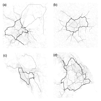
Figure 4: We show for real-world networks the links $e$ with a BC larger than a certain threshold $g(e)>g^{*}$ and we highlight the largest loop. (a) Dresden, Germany ($g^{*}=0.11$). (b) Paris, France ($g^{*}=0.315$). (c) Los Angeles, USA ($g^{*}=0.05$). (d) Shanghai ($g^{*}=0.07$).

For all these real-world cases, we observe that indeed non-trivial structures appear and in particular we observe the appearance of loops made of central links and of different sizes. We can test the stability of these loops, by filtering these networks for different values of the BC threshold $g^{*}$ and compute the perimeter of the main loop. The results for Dresden, Los Angeles, and Paris are shown in Fig. 5.

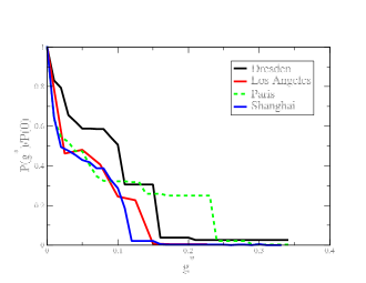
Figure 5: Perimeter $P(g^{*})$ of the main loop (normalized by perimeter of the loop at $g^{*}=0$) for the road network of Dresden, Los Angeles, and Paris.

We observe on this plot the presence of various plateaus at intermediate values of $g^{*}$ suggesting that these loops are indeed very central and stable.

In general, boundary effects can be important and can affect the measures done on spatial networks Rheinwalt:2012 . In general, the choice of boundaries has an impact on quantities such as the BC Gil:2016 and we briefly discuss this problem here. We measure the area enclosed in the largest loop on the same network but at different scales (ie. with different boundaries, going from central Paris to almost the whole Ile-de-France region) and the results are presented in Fig. 6.

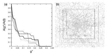
Figure 6: (a) Normalized area $A(g^{*})$ defined by the largest loop for different boundary conditions on the Paris road network. The lowest curve corresponds to the largest size and for decreasing size the curves are shifted to larger values of the area. (b) Different boundaries corresponding to the curves of (a).

In this figure, we observe that at least the area of the largest loop remains relatively stable. Further systematic studies are however certainly needed in order to understand which patterns are stable and which ones are not, and what are the conditions on the boundaries in order to ensure stability of the main spatial patterns.

II.5 Summary: stylized facts

These different examples discussed above show that the introduction of disorder in planar graphs induce in general the formation of non-trivial structures made of links with a large BC. In particular, we observe the appearance of loops made of links that can have a BC larger than the barycenter. In other words, disorder can invert the typical behavior observed for regular lattice where the BC is decreasing monotonously from the barycenter. In the following, we propose a toy model which allows to discuss and to understand under which conditions a loop can become more central than the spatial center.

III Theoretical approach: A toy model

As discussed above, we observe that non-trivial objects such as loops can be very central in random graphs. It is important to understand the formation of these structures and the conditions for their existence. In particular, it seems that randomness can induce very large perturbation in the spatial distribution of the BC and where the barycenter is not the most central node. Equivalently, the BC could not be a simple decreasing function of the distance to the barycenter anymore. In order to understand this phenomenon, we propose here a simple toy model. We first construct a star network composed of $N_{b}$ branches, where each branch is composed of $n$ nodes. We then add a loop at distance $\ell$ from the center (see Fig. 7 for a sketch of this graph). We also consider here a more general case where the links are weighted and in this simplified model we assume that links have a weight equal to one and the loop segment between two consecutive branches has a weight given by $w$. The purely topological case then corresponds to the case $w=1$. We then compute the BC using weighted shortest paths. This generalization allows us to discuss for example the impact of different velocities on a street network. In this case, $w$ can be seen as the time spent on the segment and the weighted shortest path is then the quickest path.

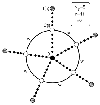
Figure 7: Representation of the toy model discussed here. The number of branches is here $N_{b}=5$, the number of nodes on each branch is $n=11$ and the loop is located at a distance $\ell=6$ from the center $0$. The node $C$ is at the intersection of a branch and the loop and $T$ is the terminal node of a branch.

Here, we want to discuss under which conditions the loop will be more central than the ‘origin’ at the center in this simplified network. Intuitively, for very large $w$, it is always less costly to avoid the loop, while for $w\to 0$, loops are very advantageous. The two main quantities of interest are therefore the centrality at the center denoted by $g_{0}(\ell,n,w)$ and the centrality, denoted by $g_{C}(\ell,n,w)$, at the intersection $C$ of the branch and the loop. We then compute the difference $\delta g=g_{0}-g_{C}$ and will study under which condition it can be negative.

III.1 Exact and approximated formulas

The interest of this toy model lies in the fact that we can estimate analytically the BC for the center $g_{0}(\ell,w)$ and for the intersection nodes on the loop $g_{C}(\ell,w)$. Formally we can write these quantities as

$$g_{0}(\ell,n,w) =g_{0}(\ell,n,\infty)-(a_{1}^{0}+a_{2}^{0}+a_{3}^{0})$$

$$g_{C}(\ell,n,w) =g_{C}(\ell,n,\infty)+(a_{1}^{C}+a_{2}^{C}+a_{3}^{C})$$ (5)

where the $a_{x}^{i}$ are positive. We distinguish two parts in these centralities. First, we estimate the BC when there is no loop which is represented by the case where $w\to\infty$. This part is modified by the presence of the loop that under certain conditions can be more interesting for connecting pairs of nodes. We can understand the signs in Eq. 5, by noting that the presence of the loop will decrease the centrality at the center and increase the centrality at $C$. The different terms $a_{i}^{x}$ (where $x=0,C$ and $i=1,2,3$) count the paths (that avoid $0$) connecting two nodes that lie on different parts of their branch. We divide the nodes on a branch in two parts - the lower part comprises all nodes that are ‘below’ the loop $0<s<\ell$ and the upper part is the rest $\ell<s\leq n$. When both nodes are on the upper part of the branches we obtain $a_{1}^{x}$; the paths connecting an upper part to a lower part are described by $a_{2}^{x}$ and when both nodes lie on a lower part, we obtain the coefficient $a_{3}^{x}$. For more details and the calculation of these coefficients, we refer to the appendix.

The exact expressions for the centralities $g_{0}$ and $g_{C}$ are however difficult to handle analytically, essentially because they are expressed as sums of complicated arguments (see appendix). In order to derive analytical predictions we will propose in the following a simple approximation scheme that allows to obtain the correct scalings for the most important quantities.

In the derivation of the exact expression of the centralities Eq. 5, we have to distinguish different cases according to the value of

$$\chi\equiv\min\left(\frac{N_{b}-1}{2},\left[\frac{2\ell}{w}\right]\right)$$ (6)

compared to $j-1$ (the brackets $[\cdot]$ denote here the integer part, ie. the lowest nearest integer) which denotes the number of loop segments between the first branch and the branch $j$. This essentially amounts to compare the cost of the path between a node on the lower part (with $0<s<\ell$) of the first branch $B_{1}$ to a node on the lower part ($0<t<\ell$) of another branch $B_{j}$. If $[2\ell/w]>j-1$ the cost of the path which goes through $0$ is larger than going directly via the loop (given by $(j-1)w$) and therefore produces a negative contribution to $g_{0}$. We see that this discussion allows to distinguish for a given value of $w$ ‘near’ from ‘far-away’ branches (Fig. 8). The nearest branches are then defined by the condition $j-1\leq\chi$ and the remote branches by $\chi<j-1\leq(N_{b}-1)/2$ (for simplicity we assume here that $N_{b}$ is odd and by symmetry we can discuss only one half for the branches from $j=2$ to $j=(N_{b}-1)/2$).

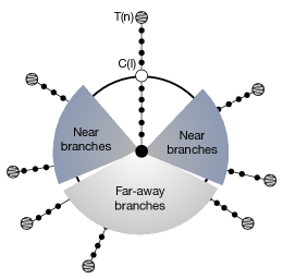
Figure 8: Schematic representation of the approximation used to compute the centrality $g_{0}(w)$ at the center $0$.

We will then use the following simplification: we will assume that for the $\chi$ near branches, going through the center is always the best choice for $s<\ell$ and $t<\ell$ while for all other paths (from or to an upper path) it is beneficial to go through the loop. This leads then to

$$g_{near}=\chi\frac{(\ell-1)(\ell-2)}{2}$$ (7)

For the $(N_{b}-1)/2-\chi$ far-away branches, we consider that for all nodes $s,t\in\llbracket 1,n\rrbracket$, the paths are going through the center leading to

$$g_{far}=\left(\frac{N_{b}-1}{2}-\chi\right)n^{2}$$ (8)

Taking into account the factor $2$ for not counting twice the same path, we obtain for $g_{0}(w)=N_{b}(g_{near}+g_{far})$ the following expression

$$g_{0}(w)\approx N_{b}\left\{\left(\frac{N_{b}-1}{2}-\chi\right)n^{2}+\chi\frac{(\ell-1)(\ell-2)}{2}\right\}$$ (9)

We note that this approximation recovers both exact limits

$$g_{0}\simeq\begin{cases}N_{b}\frac{(N_{b}-1)}{2}\frac{(\ell-1)(\ell-2)}{2}&\;\mathrm{for}\;w\to 0\\ n^{2}N_{b}\frac{(N_{b}-1)}{2}&\;\mathrm{for}\;w\to\infty\end{cases}$$ (10)

In the following it will also be useful to consider the limit $\ell,n\to\infty$ with $x=\ell/n$ fixed which gives for $g_{0}(x,\chi)=g_{0}(\ell,n,w)/n^{2}$ (up to terms of order $1/n$)

$$g_{0}(x,\chi)\approx N_{b}\left\{\left(\frac{N_{b}-1}{2}-\chi\right)+\frac{1}{2}\chi x^{2}\right\}$$ (11)

where the only dependence on $w$ is now encoded in $\chi$, hence the change of argument for clarity.

We can produce the same type of arguments for the BC on the loop. First the value without the loop is easy to compute and we obtain

$$g_{C}(\ell,n,w=\infty)=(n-\ell)\left[\ell+n(N_{b}-1)\right]$$ (12)

which simply counts the number $(n-\ell)$ of nodes ‘above’ $C$ and all the others ($C$ being excluded). Similar arguments as above then give the following result (we also changed here the argument of the function from $w$ to $\chi$)

$$g_{C}(\ell,n,\chi) =g_{C}(\ell,n,w=\infty)$$

$$+2\chi\Big{[}(n-\ell+1)(\ell-1)+\frac{(\ell-1)(\ell-2)}{2}\Big{]}$$

$$+\frac{\chi(\chi-1)}{2}\Big{[}(n-\ell+1)^{2}$$

$$+2(n-\ell+1)(\ell-1)+\frac{(\ell-1)(\ell-2)}{2}\Big{]}$$ (13)

where $\chi$ is given by Eq. 6. In particular the term proportional to $\chi$ counts all the paths between the lower part of the branch containing $C$ and all the nodes of a branch close enough. The second term (proportional to $\chi(\chi-1)$) counts the paths going from a branch $B_{j}$ with $j\in[1,\chi-1]$ to the other branches $j^{\prime}=1,2,\dots,j-1$. The sum of all these contributions gives the factor $\chi(\chi-1)/2$. The counting factor is not trivial here and comes from evaluating all the paths from a node $s$ in a branch $j$ to a node $t$ on a branch $j^{\prime}$ ($j$ and $j^{\prime}$ are different from $1$) such that

$$s+t>|\ell-s|+|\ell-t|+w\Delta j$$ (14)

The left hand side of this inequality corresponds to the distance through the center and $w\Delta j$ is the distance on the loop (for the exact expression of the centrality and how to recover this approximate formula, we refer the interested reader to the appendix).

Similarly to the case of the BC at $0$, it will be convenient for analyzing these expressions to consider the limit $n,\ell\to\infty$ such that $\ell/n=x$. Up to terms of order $1/n$ we then obtain for $g_{C}(x,\chi)=g_{C}(\ell,n,w)/n^{2}$

$$g_{C}(x,\chi) =(1-x)(x+N_{b}-1)$$

$$+2\chi x(1-\frac{x}{2})$$

$$+\frac{\chi(\chi-1)}{2}(1-\frac{x^{2}}{2})$$ (15)

We show in the figure 9 the comparison of the exact result with the approximations developed here.

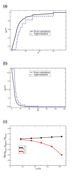
Figure 9: Comparison between the exact result and the approximation for $g_{0}(w)$ (a) and $g_{C}(w)$ (b) (the BC are here normalized). The parameter values are here $N_{b}=21$, $n=60$ and $\ell=30$. (c) Relative error between the exact value and approximation for $g_{0}$ and $g_{C}$ for $N_{b}=21$, $n=60$, $w=30$, $\ell=30$.

For large values of $\ell$ the approximation is not excellent and can certainly be improved. However as we will show in the following, our simple approximations allow to understand and to predict the correct scaling for the important quantities $\ell_{opt}$ and $w_{c}$.

III.2 Threshold value of $w$ and optimal $\ell$

The fundamental quantity that we wish to understand is the difference $\delta g(x,\chi)=g_{0}(x,\chi)-g_{C}(x,\chi)$ given by Eqs. (11,15). We first plot this quantity versus $\ell$ for different values of $w$ and we observe the result shown in Fig. 10

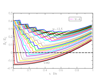
Figure 10: $\delta g(\ell)$ versus $\ell$ (for $N_{b}=15$ and $n=60$ here) and for different values of $w$ in the range $[0,12.5]$. For values less than a threshold ($w_{c}\approx 4$ shown here by a dotted line) there is a minimum that is negative.

This result shows that for $w$ sufficiently small, $\delta g$ can be negative. This demonstrates the existence of a threshold value $w_{c}$ such that at $w=w_{c}$ the minimum is $\min_{\ell}\delta g=0$. For $w<w_{c}$, the minimum of $\delta g$ is negative and we can define an optimal value $\ell_{opt}$ which corresponds to this smallest value of $\delta g$. The quantity $\ell_{opt}$ thus gives the position of loop that maximizes the difference between the BC of the loop and the center.

In order to estimate this optimal value $\ell_{opt}$, we note (using the expression Eq. 6 for $\chi$) that the difference $\delta g(x,\chi)$ gives

$$\delta g(x,\chi)=\begin{cases}\delta g(x,\frac{2\ell}{w})&\;\mathrm{for}\;\ell\in[0,\frac{(N_{b}-1)w}{4}]\\ \delta g(x,\frac{N_{b}-1}{2})&\;\mathrm{for}\;\ell\in[\frac{(N_{b}-1)w}{4},2n]\end{cases}$$ (16)

In order to discuss to estimate analytically both the threshold $w_{c}$ and the optimal value $\ell_{opt}$, we will use equations Eqs. (11,15) and study the approximate difference $\delta g(x,\chi)=g_{0}(x,\chi)-g_{C}(x,\chi)$ given by

$$\delta g(x,\chi) =N_{b}\left[\frac{N_{b}-1}{2}-\chi+\frac{1}{2}\chi x^{2}\right]$$

$$-(1-x)(x+N_{b}-1)-2\chi x(1-\frac{x}{2})$$

$$-\frac{\chi(\chi-1)}{2}(1-\frac{x^{2}}{2})$$ (17)

We first study the derivative with respect to $\ell$ of this difference in the domain $\ell<[(N_{b}-1)w/4]$. After simple calculations we obtain that for large $N_{b}$ and $n$ (we treat here $\ell$ as a continuous variable) $\mathrm{d}\delta g/\mathrm{d}\ell<0$ in the domain considered. A similar calculation shows that in the domain $(N_{b}-1)/4<\ell<2n$, the function $\delta g(\ell,n,\chi)$ is increasing with $\ell$ (at least for $N_{b}$ large enough). These results thus show that the minimum of $\delta g$ is actually reached at the intersection of the two curves and which occurs for

$$\ell_{opt}=\frac{(N_{b}-1)w}{4}$$ (18)

This expression for $\ell_{opt}$ is actually independent from the exact form of $\delta g$ as long as it is decreasing for $\ell<\ell_{opt}$ and increasing above $\ell_{opt}$ which we verified numerically. We compare the theoretical prediction Eq. (18) with numerical results in Fig. 11,

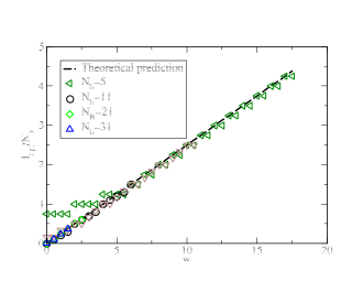
Figure 11: Comparison between the theoretical prediction (Eq. 18) and numerical results for $\ell_{opt}$ (for $w<w_{c}$). For large value of $N_{b}$ the prediction is excellent. We note that $\ell_{opt}$ exists for $w<w_{c}$ and $w_{c}$ decreases with $N_{b}$ which implies that the range over which we can see a linear behavior is decreasing as $1/N_{b}$ (here $n=40$).

and we see that for $N_{b}$ large enough (here, typically $N_{b}>10$) this prediction is in excellent agreement with data.

We can understand this value of $\ell_{opt}$ with the following simple argument. If $\ell$ is small most paths connecting nodes from different branches will go through $0$ and we expect $\delta g>0$. When $\ell$ is increasing more paths will go through the loop and will increase the value of $g_{C}$. However, when $\ell$ is too large, paths connecting the (large) fraction of nodes located on the lower branches will go through $0$ again. In order to get a sufficient condition on $\ell_{opt}$, we consider the path between the node $C$ on the branch $B_{1}$ and the corresponding node $C^{\prime}$ on the furthest branch $(N_{b}-1)/2$. The optimal value for $\ell_{opt}$ is then such that the cost of the path from $C$ to $C^{\prime}$ through $0$ and which is $2\ell$ is equal to the cost on the loop which is given by $w(N_{b}-1)/2$. This immediately gives the result $\ell_{opt}\approx w(N_{b}-1)/4$.

The threshold quantity $w_{c}$ is obtained by imposing that the minimum of $\delta g(\ell=\ell_{opt})$ is equal to zero. Using the approximate form Eq. 17, we can show that the minimum is actually obtained for $\ell=\ell_{opt}$ and for $\chi=(N_{b}-1)/2$. We thus have to consider the quantity $\delta g(\ell_{opt},n,\chi=(N_{b}-1)/2)$ which for large $N_{b}$ is behaving as large $N_{b}$

$$\delta g(\ell_{opt})\approx\frac{N_{b}^{2}}{8}\left[\frac{5}{2}\left(\frac{wN_{b}}{4n}\right)^{2}-1\right]$$ (19)

(details of this calculation are given in appendix) and we therefore obtain

$$w_{c}\approx\kappa\frac{n}{N_{b}}$$ (20)

where $\kappa=4\sqrt{\frac{2}{5}}$ in this approximation.

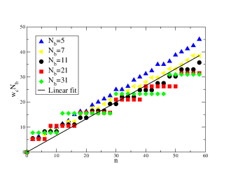
Figure 12: Value of $w_{c}N_{b}$ versus $n$. The collapse is reasonably good and is in agreement with our theoretical result Eq. 20. We observe plateaus that are due to the discrete values of $\ell$ and $n$. The straight line is a linear fit which gives $\kappa_{emp}\approx 0.66$ ($r^{2}=0.96$).

We can understand the scaling for $w_{c}$ with the simple following argument. Indeed, a necessary condition on $w$ is that $\ell_{opt}$ must be less than $n$. This gives the condition

$$w<\widetilde{w}_{c}=4\frac{n}{N_{b}}$$ (21)

This threshold $\widetilde{w}_{c}$ is a priori larger than the exact value, as we imposed here a necessary condition, but allows to understand in a simple way the scaling of $w_{c}$ with $n$ and $N_{b}$. We test the scaling for $w_{c}$ by plotting (Fig. 12) $w_{c}N_{b}$ versus $n$ and which should be linear. We indeed observe a reasonable agreement with the linear behavior predicted by our analysis, where the differences are probably due to the small values of $N_{b}$ used for the numerical calculations. The linear fit however gives a prefactor $\kappa_{emp}\approx 0.66$ which is far from the value obtained within our simple approximation scheme. The important fact is that our approximation is able to predict the correct scaling and it could maybe be possible to find more refined approximations in order to get a better estimate for the prefactor $\kappa$. Finally, we note here that $w_{c}$ is independent from $\ell$ which can be understood by the fact that $w_{c}$ gives a condition for the existence of $\ell_{opt}<n$.

Finally, we note that when $w_{c}>1$, the case $w=1$ displays then a negative minimum and we can observe a very central loop. This case is particularly interesting as it corresponds to the ‘topological’ case for which the distance is the minimum number of hops. This will then happen when there are few branches, or if the branches are large enough.

IV Discussion

The main purpose of this paper is to shed light on the appearance of non-trivial patterns made of very central nodes (or links) in real-world planar graphs. In particular, we focused on the existence of very central loops that are commonly observed in random planar graphs. We proposed a toy model that shows that indeed a loop at a certain distance from the center can be more central than the physical center itself. The condition for the existence of such a phenomenon is that the weight on the loop has to be small enough and in this toy model we showed the existence of a threshold value $w_{c}$. This threshold depends on the size and number of radial branches, highlighting their crucial role. This result allows us to understand the appearance of very central loop even in the topological case where the shortest topological distance is used for computing the BC: if the extension of the network is large compared to the number of radial branches, $w_{c}$ can be larger than one $w_{c}>1$ and central loops for $w=1$ can be observed. In ordered systems – such as lattices – the effective number of branches is too large leading to a very small $w_{c}$ and therefore prohibits the appearance of central loops in the ‘topological’ case ($w=1$). In real-world planar graphs where randomness is present, the absence of some links can lead to a small number of ‘effective’ radial branches which in the framework of the toy model implies a large value of $w_{c}$ and therefore a large probability to observe central loops.

In the case of roads, if we assume that the weight is inversely proportional to the velocity, our result predicts that the velocity on the loop has to be large enough in order to be very central and faster than going through the center. A possible direction of future studies could then to include more precisely different velocities and also to include congestion effects.

More generally, further studies are needed in order to understand the variety of patterns induced by randomness in planar graphs, and we believe that this study is a step towards this direction.

V Acknowledgements

BL and MB thank Jean-Marc Luck for interesting discussions and valuable suggestions. MB thanks Gourab Ghoshal for stimulating exchanges on this problem.

VI Appendix

VI.1 BC at the center

VI.1.1 Complete formula

The general expression for the BC at the center is

$$g_{0}(w)=n^{2}N_{b}(N_{b}-1)/2-(a_{1}^{0}+a_{2}^{0}+a_{3}^{0})$$ (22)

In order to analyze this quantity, we separate the branches into two parts. The first part is composed of nodes at a distance lower than $l$ from the center (the ‘lower’ part of the branch), and the second part consists in nodes that are at a distance greater or equal than $l$ from the center (the ‘upper’ part of the branch). When there is no loop, the total number of shortest paths going through the center is ($N_{tot}$ denotes the total number of nodes)

$$g_{0}(w=\infty) =\dbinom{N_{tot}-1}{2}-\dbinom{n}{2}\cdot{N_{b}}$$

$$=n^{2}N_{b}(N_{b}-1)/2$$ (23)

This expression gives the betweenness centrality at the center without the loop, and we can calculate $g_{0}(w)$ by removing from $g_{0}(\infty)$ all the shortest paths that go through the loop and not through the center. This can be computed by distinguishing different types of paths: the quantity $a_{1}^{0}$ counts the number of shortest paths going through the loop and connecting nodes both located on the upper part of branches; the quantity $a_{2}^{0}$ counts these paths connecting an upper part to a lower one; and $a_{3}^{0}$ counts the paths connecting nodes both located in lower parts of branches.

We note that due to the symmetry of this network, it is enough to consider paths from a given branch to the others and to multiply at the end of the calculation by the number of branches.

The central point for calculating the centralities $g_{0}(w)$ and $g_{C}(w)$ is to compare the length of the path through $0$ and the path through the loop. For a node located at distance $s$ on branch $0$ and a node at distance $t$ on a branch $j$ (where $j$ goes from $1$ to $N_{b}-1$), this condition can be written as

$$s+t<|\ell-s|+|\ell-t|+wj$$ (24)

If this inequality is satisfied the path will go through $0$ and otherwise the loop is more interesting. We thus have to count the pair of nodes that satisfies this inequality and for this we distinguish three different cases: $s$ and $t$ in the lower part of branches, $s$ and $t$ in the lower and upper parts respectively, and finally both $s$ and $t$ in the upper part of branches. In the following we introduce two quantities:

$$X_{j}=\min\left(\left[\frac{2j}{w}\right],\frac{N_{b}-1}{2}\right)$$ (25)

and

$$P_{j} =\frac{1}{2}\theta(N_{b}\;\;\mathrm{odd})\theta(\frac{2j}{w}=X_{j})$$

$$+\theta(N_{b}\;\;\mathrm{even})\left(\frac{2}{3}\theta(\frac{N_{b}}{2}=\frac{2j}{w})+\frac{1}{2}\theta(\frac{N_{b}}{2}<\frac{2j}{w})\right)$$

where $\theta(condition)=1$ if condition is true, and is $0$ otherwise. This quantity $P_{j}$ takes into account the fact that the shortest path going through the center or through the loop have the same length. If $2j/w=X_{j}$ we have to divide by two the number of paths and $X_{j}-P_{j}$ is the fraction of paths going through the center. In addition, if $N_{b}$ is even and $N_{b}/2=2j/w$, we have $3$ different paths with the same length that connect two nodes on opposite branches: one path through the center, another 2 paths on each direction of the loop. In this case, there are $2/3$ of paths to remove in order to get $g_{0}$. in each case $X_{j}-P_{j}$ multiplies the total flow.

Calculation of $a_{1}^{0}$

There are $(n-\ell+1)$ nodes in the upper part of one branch and therefore $N_{b}(n-\ell+1)^{2}$ possible pairs between two nodes of two distincts upper parts. The number of branches with nodes that will deviate from the center and will use the loop is given by $X_{\ell}$. We have however to consider cases where there are shortest paths that equivalently go through the center or via the loop, and this is precisely what is counted by $P_{\ell}$. The coefficient $a_{1}^{0}$ is then given by

$$a_{1}^{0}=N_{b}(n-\ell+1)^{2}(X_{\ell}-P_{\ell})$$ (26)

We can recover this result by noting that for nodes $s$ and $t$ belonging to the upper part of different branches $B_{1}$ and $B_{j}$, the condition that the path through the center is longer than on the loop is

$$s+t>s-\ell+t-\ell+wj$$ (27)

which leads to $2\ell>wj$ and a number of branches given by $[2\ell/w]=X_{\ell}$. We have an equality when $2\ell=wj$ and this happen when $X_{\ell}=2\ell/w$ and gives a factor $1/2$ in the BC.

Calculation of $a_{2}^{0}$

For the $a_{2}^{0}$ coefficient, only paths between the lower part and the upper part are considered. We consider a node (in the first branch) in the lower part $s<\ell$ and another one in the upper part on $t>\ell$ in the branch $j$. The path from $s$ to $t$ is deviated from zero if the following condition is met

$$s+t>|\ell-s|+|\ell-t|+wj$$

$$\Rightarrow 2s>wj$$ (28)

which means that the number of such paths is given by the number of nodes in the upper part $(n-\ell+1)$ times the number of branches that satisfy this condition: $j<\left[\frac{2s}{w}\right]$. We have to sum over $s\in\llbracket 1,\ell\rrbracket$ and to multiply by $2N_{b}$ which takes into account both paths (from the upper to the lower and from the lower to the upper part of branches) and obtain

$$a_{2}^{0}=2N_{b}(n-\ell+1)\sum_{s=1}^{\ell-1}(X_{s}-P_{s})$$ (29)

(the term $P_{s}$ takes into account the degeneracies of paths).

Calculation of $a_{3}^{0}$

The quantity $a_{3}^{0}$ represents deviation between pairs of nodes both located in the lower part of branches. in this case, the condition on paths is

$$s+t>\ell-s+\ell-t+wj$$ (30)

which implies that the branches where we have a deviation from $0$ are such that

$$j<\frac{2(s+t-\ell)}{w}$$ (31)

and we then obtain

$$a_{3}^{0}=N_{b}\sum_{s=1}^{\ell-1}\sum_{t=1}^{s-1}(X_{s+t-\ell}-P_{s+t-\ell})$$ (32)

We therefore finally obtain the exact expression

$$g_{0}(w)\approx n^{2}N_{b}(N_{b}-1)/2-(a_{1}+a_{2}+a_{3})$$ (33)

with

$$a_{1}=N_{b}(n-\ell+1)^{2}\cdot(X_{\ell}-P_{\ell})$$ (34)

$$a_{2}=2N_{b}(n-\ell+1)\sum_{s=1}^{\ell-1}(X_{s}-P_{s})$$ (35)

$$a_{3}=N_{b}\sum_{s=1}^{\ell-1}\sum_{t=1}^{s-1}(X_{s+t-\ell}-P_{s+t-\ell})$$ (36)

where $X_{j}=\min(\left[\frac{2j}{w}\right],\frac{N_{b}-1}{2})$ and $P_{j}$ given above. The sums entering these expressions are however difficult to handle and we therefore resort to approximations that are detailed in the main text.

VI.1.2 Simplification

Another way to recover the approximation discussed in the main text is to neglect small deviation terms (ie. to impose $P_{j}=0$), and we then obtain

$$g_{0}(w)\approx n^{2}N_{b}(N_{b}-1)/2-(a_{1}+a_{2}+a_{3})$$ (37)

with

$$a_{1}=N_{b}(n-\ell+1)^{2}\cdot X_{\ell}$$ (38)

$$a_{2}=2N_{b}(n-\ell+1)\sum_{s=1}^{\ell-1}X_{s}$$ (39)

$$a_{3}=N_{b}\sum_{s=1}^{\ell-1}\sum_{t=1}^{s-1}X_{s+t-\ell}$$ (40)

We are still left with the sums to compute and the simplest approximation we can think of (and that can be used for $g_{C}$ too) is to choose $X_{j}\approx X_{\ell}=\chi$ leading to

$$a_{1}\approx N_{b}(n-\ell+1)^{2}\chi$$ (41)

$$a_{2}\approx 2N_{b}(n-\ell+1)\chi(\ell-1)$$ (42)

$$a_{3}\approx N_{b}\chi\frac{(\ell-2)(\ell-1)}{2}$$ (43)

leading to the result Eq. 11 (in the limit $n,\ell\to\infty$ with $x=\ell/n$ fixed). This is obviously a very crude approximation and it could certainly be refined in order to get a more accurate expression for $g_{0}$. However, as we will see in the next section, the expression for $g_{C}$ is much more involved and we need an approximation scheme that can be applied to both quantities $g_{0}$ and $g_{C}$, which seems to be a difficult task that we leave for future studies.

VI.2 BC for the loop

VI.2.1 Complete formula

The first term $g_{C}(w=\infty)=(n-\ell)(n(N_{b}-1)+\ell)$ is the number of shortest path passing through $C$ when there is no loop. The quantity $(n-\ell)$ is the number of nodes in the upper part of the branch $B_{1}$ and the number of node in the rest of the network is $(n(N_{b}-1)+\ell)$. Similarly as for $g_{0}$, we start from the quantity computed for $w=\infty$ and add the number of paths that will go through the loop and obtain

$$g_{C}(w)=(n-\ell)(n(N_{b}-1)+\ell)+(a_{1}^{C}+a_{2}^{C}+a_{3}^{C})$$ (44)

The first term is considering only deviation from the upper part of the branches to other upper parts. For all other branches $k=2,\dots,N_{b}/2$ (by symmetry and for $N_{b}$ even), if $wk<2\ell$, there are $((k-1)*(n-\ell+1)*(n-\ell+1))$ additional shortest paths going via the loop. By summing over $k$ and taking into account multiple paths, we obtain

$$a_{1}^{C}=(n-\ell+1)^{2}(\frac{1}{2}(X_{\ell-w/2}+1)X_{\ell-w/2}-P_{\ell}^{1})$$ (45)

The coefficient $a_{2}^{C}$ counts the paths from the upper part of a branch to the lower part of another branch. This path will go through the loop if $wi<2j$ with $i$ going from $1$ to $N_{b}/2$ and $j$ from $1$ to $\ell-1$. We then obtain

$$a_{2}^{C}=2(n-\ell+1)\sum_{j=1}^{\ell-1}\left(\frac{X_{j}(X_{j}+1)}{2}-P_{j}^{2}\right)$$ (46)

Finally, the coefficient $a_{3}^{C}$ corresponds to additional shortest paths from lower part to lower part and going through the loop. When $wi<2(j+k-\ell)$, with $i=1,\dots,N_{b}/2$, $j=1,\dots,\ell-1$, and $k$ running from $\ell-j+1$ to $\ell-1$, there are $(i+1)$ new shortest paths added at point C. Summing over $i$, we then obtain

$$a_{3}^{C}=\sum_{j=1}^{\ell-1}\sum_{k=1}^{j-1}\left(\frac{X_{j+k-\ell}(X_{j+k-\ell}+3)}{2}-P_{j+k-\ell}^{3}\right)$$ (47)

The quantities $P_{j}^{i},\;i=1,...,3$ correspond to the correction needed when the path going through the loop has the same weight as the path going through $0$.

For the part $1$:

$$P^{1}_{j} =\frac{X_{j}}{2}\theta(\frac{2j}{w}=X_{j})\theta(\frac{N_{b}}{2}\neq X_{j})$$

$$+\frac{N_{b}/2-1}{3}\theta(\frac{N_{b}/2}{2}=\frac{2j}{w})\theta(\frac{N_{b}}{2}=\left[\frac{N_{b}}{2}\right]$$

$$+\frac{N_{b}/2-1}{2}\theta(\frac{N_{b}}{2}<\frac{2j}{w})\theta(\frac{N_{b}}{2}=\left[\frac{N_{b}}{2}\right])$$ (48)

For the part $2$:

$$P^{2}_{j} =\frac{X_{j}}{2}\theta(\frac{2j}{w}=x_{j})\theta(\frac{N_{b}}{2}\neq X_{j})$$

$$+\frac{2(N_{b}/2)}{3}\theta(\frac{nb}{2}=\frac{2j}{w})\theta(\frac{N_{b}}{2}=\left[\frac{N_{b}}{2}\right])$$

$$+\frac{N_{b}/2}{2}\theta(\frac{N_{b}}{2}<\frac{2j}{w})\theta(\frac{N_{b}}{2}=\left[\frac{N_{b}}{2}\right])$$ (49)

For the part $3$:

$$P^{3}_{j} =\frac{X_{j}+1}{2}\theta(\frac{2j}{w}=X_{j})\theta(\frac{N_{b}}{2}\neq X_{j})$$

$$+\frac{2X_{j}+2}{3}\theta(\frac{N_{b}}{2}=\frac{2j}{w})\theta(\frac{N_{b}}{2}=\left[\frac{N_{b}}{2}\right])$$

$$+\frac{X_{j}}{2}\theta(\frac{N_{b}}{2}<\frac{2j}{w})\theta(\frac{N_{b}}{2}=\left[\frac{N_{b}}{2}\right])$$ (50)

VI.2.2 Simplification

Here also, we can recover the approximate formula (Eq. 15) by using the same approximation as described above for $g_{0}$: we neglect small deviation terms ($P_{j}=0$) and we assume that $X_{j}=X_{\ell}\approx\chi$ for all $j$ which gives

$$g_{C}(w)=(n-\ell)(n(N_{b}-1)+\ell)+(a_{1}^{C}+a_{2}^{C}+a_{3}^{C})$$ (51)

with

$$a_{1}^{C} =(n-\ell+1)^{2}\frac{1}{2}(X_{\ell-w/2}+1)X_{\ell-w/2}$$

$$\approx(n-\ell+1)^{2}\frac{\chi(\chi-1)}{2}$$ (52)

$$a_{2}^{C} =2(n-\ell+1)\sum_{j=1}^{\ell-1}\frac{X_{j}(X_{j}+1)}{2}$$

$$\approx 2(n-\ell+1)(\ell-1)\frac{\chi(\chi+1)}{2}$$ (53)

$$a_{3}^{C} =\sum_{j=1}^{\ell-1}\sum_{k=1}^{j-1}\frac{X_{j+k-\ell}(X_{j+k-\ell}+3)}{2}$$

$$\approx\frac{\chi(\chi+3)}{2}\;\frac{(\ell-2)(\ell-1)}{2}$$ (54)

where $\chi=\min(\left[\frac{2j}{w}\right],\frac{N_{b}-1}{2})$. Summing all these terms and taking the limit $n,\ell\to\infty$ with $\ell/n=x$ fixed, we recover the approximation Eq.15.

VI.3 Calculation of $w_{c}$

We start with the expression Eq. 17

$$\delta g(x,w) =N_{b}\left[\frac{N_{b}-1}{2}-\chi+\frac{1}{2}\chi x^{2}\right]$$

$$-(1-x)(x+N_{b}-1)-2\chi x(1-\frac{x}{2})$$

$$-\frac{\chi(\chi-1)}{2}(1-\frac{x^{2}}{2})$$ (55)

where $\chi=\frac{N_{b}-1}{2}$. In the limit $N_{b}\gg(x-1)$ we obtain (keeping terms growing with $N_{b}$)

$$\delta g(x,w)\simeq N_{b}\left[\frac{N_{b}-1}{4}x^{2}\right]$$

$$-(1-x)N_{b}-2\frac{N_{b}-1}{2}x(1-\frac{x}{2})$$

$$-\frac{N_{b}-1}{4}(\frac{N_{b}-1}{2}-1)(1-\frac{x^{2}}{2})$$

which behaves at leading order as

$$\delta g(x,w)\simeq\frac{N_{b}^{2}}{8}\left(\frac{5}{2}x^{2}-1\right)$$ (56)

The minimum is crossing zero at

$$x^{2}=\frac{2}{5}$$ (57)

which implies for $\ell=\ell_{opt}\simeq N_{b}w/4$

$$w_{c}\simeq\sqrt{\frac{2}{5}}\frac{4n}{N_{b}}$$ (58)

References

- (1) Clark, J., Holton, D. A. A first look at graph theory (Vol. 1). Teaneck, NJ: World Scientific (1991).
- (2) Tutte, W.T. A census of planar maps. Canad. J. Math 15, 249-271 (1963).
- (3) Bouttier, J., Di Francesco, P. & Guitter, E. Planar maps as labeled mobiles. Electron. J. Combin 11, R69 (2004).
- (4) Ambjorn, J. & Jonsson, P. Quantum geometry: a statistical field theory approach (Cambridge University Press, Cambridge, UK, 1997).
- (5) Mileyko, Y., Edelsbrunner, H., Price, C.A. & Weitz J.S. Hierarchical ordering of reticular networks. PLoS One 7, e36715 (2012).
- (6) Katifori, E. & Magnasco, M.O. Quantifying loopy network architectures. PLoS One 7, e37994 (2012).
- (7) Katifori, E., Szollosi GJ, Magnasco, M.O. Damage and fluctuations induce loops in optimal transport networks. Physical Review Letters 104:048704 (2010).
- (8) Hu, D., Cai, D. Adaptation and optimization of biological transport networks. Physical review letters 111:138701 (2013).
- (9) Barthelemy, M. Spatial Networks. Phys. Rep. 499, 1-101 (2011).
- (10) Haggett, P. & Chorley, R.J. 1969 Network analysis in geography. London: Edward Arnold.
- (11) Hillier, B., Hanson, J. The social logic of space (Vol. 1). Cambridge: Cambridge university press (1984).
- (12) Marshall, S. 2006 Streets and Patterns. Abingdon: Spon Press.
- (13) B. Jiang & C. Claramunt 2004 Topological analysis of urban street networks. Environment and Planning B : Planning and design 31, 151-162.
- (14) Roswall, M., Trusina, A., Minnhagen, P. & Sneppen, K. 2005 Networks and cities: an information perspective Phys. Rev. Lett. 94, 028701.
- (15) Porta, S., Crucitti, P. & Latora, V. 2006 The network analysis of urban streets: a primal approach. Environment and Planning B: Planning and Design 33, 705–72.
- (16) Porta, S., Crucitti, P. & Latora, V. 2006 The network analysis of urban streets: a dual approach Physica A 369, 853–866.
- (17) Lammer, S., Gehlsen, B. & Helbing, D. 2006 Scaling laws in the spatial structure of urban road networks. Physica A 363, 89–95.
- (18) Crucitti, P., Latora, V. & Porta, S. 2006 Centrality measures in spatial networks of urban streets. Phy. Rev. E 73, 0361251-5.
- (19) Cardillo, A., Scellato, S., Latora, V. & Porta, S. 2006 Structural properties of planar graphs of urban street patterns. Phys. Rev. E 73, 066107.
- (20) Xie, F. & Levinson, D. 2007 Measuring the structure of road networks. Geographical Analysis 39, 336–356.
- (21) Jiang, B. 2007 A topological pattern of urban street networks: universality and peculiarity Physica A 384, 647–655.
- (22) Masucci, A. P., Smith, D., Crooks, A. & Batty, M. 2009 Random planar graphs and the London street network Eur. Phys. J. B 71, 259–271.
- (23) Chan, S. H. Y., Donner, R. V. & Lammer, S. 2011 Urban road networks- spatial networks with universal geometric features? Eur. Phys. J. B 84, 563–577.
- (24) Courtat, T., Gloaguen, C. & Douady, S. 2011 Mathematics and morphogenesis of cities: A geometrical approach. Phys. Rev. E 83, 036106.
- (25) Strano, E., Nicosia, V., Latora, V., Porta, S. & Barthelemy, M. 2012 Elementary processes governing the evolution of road networks. Nature Scientific Reports 2:296.
- (26) Barthelemy, M., Bordin, P., Berestycki, H. & Gribaudi, M. Self-organization versus top-down planning in the evolution of a city. Nature Scientific Reports 3:2153 (2013).
- (27) Viana, M. P., Strano, E., Bordin, P., Barthelemy, M. The simplicity of planar networks. Scientific reports, 3 (2013).
- (28) Louf, R., Barthelemy, M. A typology of street patterns. Journal of The Royal Society Interface, 11(101), 20140924 (2014).
- (29) Porta, S., Romice, O., Maxwell, J. A., Russell, P., & Baird, D. 2014 Alterations in scale: Patterns of change in main street networks across time and space Urban Studies 0042098013519833.
- (30) Aldous, D.J., Shun, J. Connected Spatial Networks over Random Points and a Route-Length Statistic. Stat. Sci. 25, 275-288 (2010).
- (31) L.C. Freeman, A set of measures of centrality based on betweenness, Sociometry 40, 35–41 (1977).
- (32) Ashton, D. J., Jarrett, T. C., Johnson, N. F. Effect of congestion costs on shortest paths through complex networks. Physical review letters 94:058701 (2005).
- (33) Jarrett, T. C., Ashton, D. J., Fricker, M., Johnson, N. F. Interplay between function and structure in complex networks. Physical Review E, 74:026116 (2006).
- (34) Jungnickel, D. Graphs, networks and algorithms. Berlin: Springer, 2008.
- (35) Brandes, U.. A faster algorithm for betweenness centrality. Journal of mathematical sociology 25:163-177 (2001).
- (36) M. Barthelemy, Betweenness Centrality in Large Complex Networks, Eur. Phys. J. B. 38:163 (2004).
- (37) Mapzen Weekly OSM Metro Extracts: https://mapzen.com/metro-extracts
- (38) Rheinwalt, A., Marwan, N., Werner, P., Gerstengarbe, F. W. Boundary effects in network measures of spatially embedded networks. Europhys. Lett., 100(2), 28002 (2012).
- (39) Gil, J. Street network analysis “edge effects”: Examining the sensitivity of centrality measures to boundary conditions. Environment and Planning B: Planning and Design, 0265813516650678 (2016).