Generalized thermalization for integrable system under quantum quench

Abstract

We investigate equilibration and generalized thermalization of the quantum Harmonic chain under local quantum quench. The quench action we consider is connecting two disjoint harmonic chains of different sizes and the system jumps between two integrable settings. We verify the validity of the Generalized Gibbs Ensemble description for this infinite dimensional Hilbert space system and also identify equilibration between the subsystems as in classical systems. Using Bogoliubov transformations, we show that the eigenstates of the system prior to the quench evolve towards the Gibbs Generalized Ensemble description. Eigenstates that are more delocalized (in the sense of inverse participation ratio) prior to the quench, tend to equilibrate more rapidly. Further, through the phase space properties of a Generalized Gibbs Ensemble and the strength of stimulated emission, we identify the necessary criterion on the initial states for such relaxation at late times and also find out the states which would potentially not be described by the Gibbs Generalized Ensemble description.

I INTRODUCTION

Thermalization of isolated quantum systems is apparently different from their classical counterparts CFLV . In a classical system, the constituent degrees of freedom interact and trade off charges to settle into a thermal equilibration configuration gogolin ; gge3 ; Polkovnikov . Within the framework of unitary quantum theory, a system in a pure state will never evolve to a thermal state. Instead, it has been suggested that thermalization of quantum systems needs to be understood through observables rather than the states themselves ergo . To go about this, we need to separately quantify equilibration and thermalization. An observable is said to equilibrate to a particular expectation value, within a timescale, if the temporal fluctuations about that value are small at most times. However, the observable is said to thermalize if it equilibrates to the quantum statistical description of the system. In the case of isolated quantum systems, the observables should equilibrate to their longtime averages which should be equivalent to their microcanonical expectation values gogolin ; gge3 ; Polkovnikov .

Although there is no fundamental understanding of thermalization in closed quantum systems, it has been proposed that the thermalization for some systems can be understood through eigenstate-thermalization hypothesis (ETH) deut ; sred ; alt ; Langen . In other words, non-integrable systems appear to obey ETH nat , while numerical studies show that integrable quantum systems equilibrate to a Generalized Gibbs Ensemble (GGE) description nat ; 1db ; *gge3; *tot; sys2 . More specifically, non-integrable systems at late times relax into a maximal entropic configuration such that energy of the systems remains conserved. This gives rise to the concept of thermalization under ergodic interpretation. On the other hand, an integrable system has many other conserved charges to be worried about, which prevent relaxation into a thermal configuration. With these conserved charges, the maximal entropy configuration turns out to be GGE rather than a true thermal form.

Naturally, there have been rigorous studies in the literature for Fermionic and Bosonic integrable systems. One of the most commonly studied models is the 1-dimensional Fermionic chain that makes a transition from non-integrable to integrable configuration Luttinger . To quantify relaxation in such a system, correlations and distributions are contrasted to the GGE description for various Heisenberg spin configurations Guan ; *Essler; *Vidmar; *Pozsgay; *Fagotti; *Fagotti2; *Pozsgay2; *Kozlowski; Luca2017 ; Aschbacher2003 ; Aschbacher2006 ; Luca2015 . To investigate GGE, in Ref. Rigol:0612415 , authors studied hardcore Bosons (HCB) on a lattice where a periodic potential was quenched to drive the system into super-fluid phase. In Refs. Caneva ; *PhysRevA.86.053615, the authors used a quasi-periodic potential in HCB and showed that the GGE description fails, if translational invariance is broken or there is localization in the system. In Refs. sys2 ; Pozsgay2 ; *Pozsgay3; *Brockmann, the effect of quenching on the ground state (and other interesting states such as Néel states) of the quasi-periodic potential and description of GGE were investigated. Energetics and transport properties of non-equilibrium states under quench action are also studied extensively Ogata ; Luca2013 ; Karrasch ; Luca2014 ; Medenjak .

Reference 1703.09516 recently introduced an alternative approach of truncated truncated GGE (tGGE) in interacting systems. Bosons with repulsive potentials are routinely studied using the Lieb-Linger (LL) model. In Ref. Caux:PRL2012 , equilibration of integrable or non-integrable systems with quantum quenching in the LL-model have been studied through numerical renormalization group approach. In quantum field theory, the adaptation of the concepts of thermalization has been attempted in Refs. Mussardo1 ; *Mussardo2; Doyon:2012bg ; Doyon:2014qsa .

As the reader may have noticed, to overcome the complexities of systematics in the study of thermalization of these systems, most of the studies in the literature have focused on finite-dimensional Hilbert space systems, unless the thermodynamic limit is taken. All such models, described above, restrict certain features of Bosonic nature for such studies. In this work, we investigate equilibration and thermalization of systems with infinite dimensional Hilbert space, even before going to the thermodynamic limit. For this purpose, we consider Bosonic lattice in a harmonic chain. Interacting bosons on a lattice, favoring certain hopping tendencies have been studied in q-deformed bosons Pozsgay0 ; Pozsgay-Eisler for certain special states. We do not consider them to be in any diverging repulsive potential or ascribe them any hardcore (or for that matter any quantum deformation) properties to rip them off from (or dilute or modify) their fundamental Bosonic property to accumulate. The system we consider consists of two harmonic chains that undergo sudden quantum quench (referred to as quench, hereafter) at an instant of time. The quench action we consider is joining the chains and evolve the chains as one combined chain. Specifically, we investigate the case where an integrable system makes a jump to another integrable configuration. Thus locally, at a single lattice site, the Hilbert space becomes infinite dimensional and the system is of free bosons (in normal modes) both before and after the quench. In other words, this is a system which remains integrable both before and after the quench. However, the sudden change of a parameter of coupling (from zero to non-zero value) changes the normal modes as well. Since the quench relates one integrable system to another in a linear fashion, the late time configuration can be studied also through Bogoliubov transformation, making it more adaptable to quantum field theoretic settings. We then study the evolution of an initial energy eigenstate for which the form of late time equilibration is debated. Evolution towards GGE is demonstrated for a system in a non-integrable system quenching to an integrable system Rigol1 . One of the main motivation for the Harmonic chain is its easy adaptability to field theoretic problems like in non-inertial or uniformly accelerated frames Mann1 ; *Mann2; *Mann3. Therefore, this also allows us to carry the study for all stationary states and in fact to their superpositions as well.

There have been earlier studies for integrable systems like fermionic chains, spin-lattice and the hydrodynamic settings with quenching (see, for instance, Refs. Antal ; *Cstro; *Bertini; *peschel; *eisler; *eisler2008; *caux2013time; *Luca2015; *viti2016; *Rentrop). Here, we study a Bosonic system under a local quench of joining two sub-chains. We propose a rather new technique to use covariance matrix to check violation of GGE description. We also check density correlation for the system under quench, for verification with the GGE description. It may be noted that density correlations as a check for GGE in LL-model were proposed in Ref. Nardis . In Ref. Langen207 , it was argued that that higher order correlators can be used to demonstrate relaxation to GGE in Bosonic systems. More detailed studies in dynamically evolving extended systems were done through correlations in Calabrese .

In our model, we consider the fate of any general state under quench for the infinite dimensional Hilbert space system. We also study the set of states which potentially may defy GGE description. In the literature, three sources of violation of GGE have been identified for a Fermionic system. First is the break down of the invariance of the lattice sys2 ; Caneva ; Wouters . Study of interesting aspects of inhomogeneous quenching was done in Kromos . Though it has been argued that such violations can be cured by introducing additional conserved charges Ilievski . Second, localization plays an important spoilsport PhysRevA.86.053615 and the third is the divergence of the charges which characterize the GGE description Kormos . In such cases, the Lagrange multipliers tend to vanish, effectively removing the memory of conservation. In this work, we try to test these violations while removing the HCB property from the lattice.

In particular, we ask the following questions:

1. What happens to the energy eigenstates of an integrable system when the system jumps to another integrable configuration?

2. Whether the system settles to an equilibrium state and if yes, to what state the system settles to?

3. whether steady states of pre-quench system develop Gibbs Ensemble characteristics at late times?

4. What is the measure of the states which exhibit the GGE picture?

We consider both Gaussian (e.g., ground state) and non-Gaussian (e.g. excited states) initial states for the quenched system. We study the evolution of such states post-quench, numerically as well as analytically. We use the properties of Bogoliubov transformation and, in the thermodynamic limit, show that the initial quantum state evolves to GGE form.

If system truly thermalizes, then the system must be completely described by the first two moments of the distribution in phase space deut ; sred . Hence, in this work, we focus on the structure of the covariance matrix to identify a necessary (not sufficient) condition for the system to be thermalized. Using this, we classify the set of initial states which will (or will not) evolve to a thermal configuration. Our analysis also provides a possible link of thermalization with delocalization in the Hilbert space similar in spirit to the classical equivalent — delocalization in the phase space for classical thermalization. Using these schemes we verify that for Bosonic systems, GGE description remains largely valid for states for which delocalization is large (studied through inverse participation ratio). However, this scheme also allows us to find states which are delocalized yet the GGE description fails, prominently because of divergence of the conserved charge. Thus our study delinks the localization in a Bosonic system from the divergence of the charges.

II THE MODEL and setup

The system we consider consists of two harmonic chains, with lattice sizes $N$ and $M$, respectively and use static boundary conditions for each block, which means $q_{1}=q_{N\text{ or }M}=0$, with $q_{i}$ depicting the oscillator at $i-$th lattice site. For large $N$, the results are independent of the choice of the boundary condition. For $t<0$, the two chains are non-interacting whose Hamiltonian is $H_{0}=H_{N}+H_{M},$ with,

$$H_{K}=\sum_{i=1}^{K}\frac{p_{i}^{2}}{2m}+\frac{1}{2}m\omega_{0}^{2}(q_{i+1}-q_{i})^{2}\quad K=N~{}\mbox{and}~{}M\,\,$$ (1)

At $t=0$ we turn on an interaction between the two chains with coupling strength $\omega_{0}$. Post quench $(t\geq 0)$, the Hamiltonian is $H=H_{0}+H_{int}$ where $H_{int}=-m\omega_{0}^{2}q_{N+1}q_{N}$. In terms of creation and annihilation operators, the Hamiltonian operators are,

$$\hat{H}_{0} = \sum_{l=1}^{N}\hbar\ \omega_{l}\left(\hat{a}^{\dagger}_{l}\hat{a}_{l}+\frac{1}{2}\right)+\sum_{l=1}^{M}\hbar\omega_{{}_{N+l}}\left(\hat{a}^{\dagger}_{{}_{N+l}}\hat{a}_{{}_{N+l}}+\frac{1}{2}\right)$$

$$\hat{H} = \hat{H}_{N}+\hat{H}_{M}+\hat{H}_{int}=\sum_{l=1}^{N+M}\hbar\omega_{l}(\hat{c}^{\dagger}_{l}\hat{c}_{l}+\frac{1}{2})\,,$$ (2)

where $\omega_{l}$’s are normal mode frequencies (see Appendix A).

Let the system be in an eigenstate $|\psi\rangle_{i}$ of the Hamiltonian $\hat{H}_{0}$. After quench, the time evolution of the system is described by the Hamiltonian 2. In order to compute the time evolution, we need to map $|\psi\rangle_{i}$ to a linear combination of the eigenstates of $\hat{H}$. Hence, to express $|\psi\rangle_{i}$ in terms of the eigenstates of $\hat{H}$ we need to,

1. Get a relationship between the creation and annihilation operators before and after the quench, and

2. Express the ground state $|0\rangle_{1}=|0\rangle_{N}\otimes|0\rangle_{M}$ of the disjoint system as a linear combination of an eigenstate of the joint system.

Other eigenstates can be obtained through the action of $\hat{a}^{\dagger}_{l}$ on $|0\rangle_{1}$.

We can relate creation and annihilation operators before and after the quench using the Bogoliubov transformations (see Appendix B). It is in general non-trivial to relate the ground state ($|0\rangle_{N}\otimes|0\rangle_{M}$) corresponding to $\hat{H}_{0}$ to the ground state corresponding to $\hat{H}$.

However, using the fact that the ground state is a Gaussian for the integrable systems, one can write the following general expression connecting the two:

$$|0\rangle_{N}\otimes|0\rangle_{M}=N_{0}e^{-\frac{F_{ij}}{2}\hat{c}^{\dagger}_{i}\hat{c}^{\dagger}_{j}+G_{ij}c_{i}c^{\dagger}_{j}+\cdots}|0\rangle_{N+M}$$ (3)

where $F_{ij},G_{ij}$ are $(N+M)\times(N+M)$ matrices. It can be seen that only $F_{ij}$ contributes to the expectation values of the physical quantities at the leading order of expansion. In order to do numerical computations, we need to take finitely many terms from the state expansion $\exp(\hat{O})=1+\hat{O}+\hat{O}^{2}/2+\cdots$, i.e. we need to collect contributions of different occupancy states in the new basis. We can see through inverse participation ratio in 1 and 1, contributions from higher states steadily fall down with larger lattice size.

$F_{ij}$ can be determined by solving the following constraint equations,

$$\hat{a}_{i}|0\rangle_{N}\otimes|0\rangle_{M}=0, \forall\,i=1,2,\ldots(N+M).$$ (4)

We expect $F_{ij}$ to be symmetric since $\hat{c}_{l}^{\dagger}$ operators commute with each other. Using these results and 3, any generic eigenstate of $\hat{H}_{0}$ is given by

$$|\psi\rangle_{\{(n_{i},n_{j})\}}=\prod_{i=1}^{N+M}\prod_{j=1}^{M}(\hat{a}^{\dagger}_{i})^{n_{i}}e^{-\frac{F_{lk}}{2}\hat{c}^{\dagger}_{l}\hat{c}^{\dagger}_{k}}|0\rangle_{N+M}.$$ (5)

Using 5 and the Bogoliubov transformations in Appendix B, we can therefore write this state as a linear combination of eigenstates of the Hamiltonian $\hat{H}$.

Numerically, we can study the time evolution with a finite number of the basis states, hence, we restrict 5 to the first order expansion of the exponential term. To study equilibrium relaxation of the system, we need to look at physical observables associated with it. We use the occupation number of the modes in one part of the disjoint system,

$$\hat{n}_{m} = \hat{a}^{\dagger}_{m}\hat{a}_{m},\ m=1,2\ldots,(N)$$ (6)

These are the conserved charges of the system and also determine the energy of the system prior to the quench. It is important to note that our interest is to consider large lattice limit in the large time limit. So mostly, we are interested in large time behaviour of the system post-quench. However, from the point of view of the further application of our results in infinite dimensional Hilbert space, we will also be studying the system in the usual thermodynamic limit (where the number of lattice sites being extremely large). Since these operators do not commute with the Hamiltonian after the quench, the time evolution is non-trivial. We also consider correlation of the number operators. Further our scheme of thermodynamical limit to be taken post the late time limit is different from what is typically done Aschbacher2003 ; Aschbacher2006 ; Bernard ; Bernard2015 ; Bernard2016 . Since we wish to explore a system which settles down to an equilibrium configuration (at least) in the late time (by making it asymptotically free or integrable) and analyze what is the end equilibrium configuration as the number of degree of freedom grows, we will first let the system evolve into a configuration under the action of quenching and will then take the large $N$ limit. This will also enable us to visualize the field theoretic generalization in time evolving scenarios more accurately, when a system asymptotically relaxes in an integrable configuration. This quantum field theoretic exercise we will pursue elsewhere.

One other aspect of this strategy is to reflect upon the nature of the Lagrange multiplier at the late time limit, which will be more justified when the post-quench system remains non-integrable. Thereafter, the evolution of the energies of the disjoint modes is,

$$E_{N}(t) = \sum_{i=1}^{N}\left[\hat{n}_{i}(t)+\frac{1}{2}\right]\hbar\omega_{i};$$ (7)

$$E_{M}(t) = \sum_{i=1}^{M}\left[\hat{n}_{N+i}(t)+\frac{1}{2}\right]\hbar\omega_{N+i}.$$

III Numerical RESULTS

We begin the system in an eigenstate of the disjoint Hamiltonian ($\hat{H}_{0}$). Once the system is quenched, the eigenstate can be written as linear combination of the normal mode eigenstates of the quenched Hamiltonian — delocalization in the Hilbert space of the quenched Hamiltonian. 1 gives the delocalization for different initial states and lattice sizes (for $N=5$ and different $M$), where $\mathcal{N}[\psi_{i}]$ is the approximate number of eigenstates involved in writing the first order approximation of 5. Delocalization in phase space has previously been studied from the point of view of thermalization sys1 and inverse participation ratio ($IPR=1/\sum_{i}p_{i}^{2},$) Murphy , where $p_{i}$ are the probability amplitudes of finding the state in post-quench eigenstate $|i\rangle$. 1 contains the plot of IPR for different states and lattice sizes.

M	$|\psi_{i}\rangle$	$\mathcal{N}[\psi_{i}]$	IPR	M	$|\psi_{i}\rangle$	$\mathcal{N}[\psi_{i}]$	IPR
10	$a^{\dagger}_{i}$	695	5.07118	10	$a^{\dagger}_{3}a^{\dagger}_{4}$	3181	19.1345
16	$a^{\dagger}_{i}$	1791	7.09398	16	$a^{\dagger}_{3}a^{\dagger}_{4}$	10858	36.6371
20	$a^{\dagger}_{i}$	2950	8.43266	20	$a^{\dagger}_{3}a^{\dagger}_{4}$	20801	51.3287

Table 1: Table shows the delocalization of initial state $\psi_{i}$ for $N=5$ and different $M$ lattice sites.

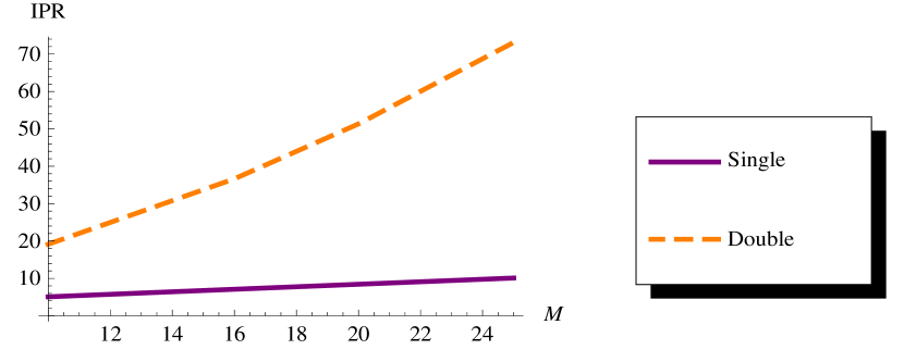
Figure 1: IPR of different states and lattice size

Equilibration, steady states and fluctuations: In order to go about understanding equilibration, we evaluate the observables $E_{N}(t),E_{M}(t),E_{N}(t)+E_{M}(t)$ as a function of time. From 2 and 3, we infer the following:

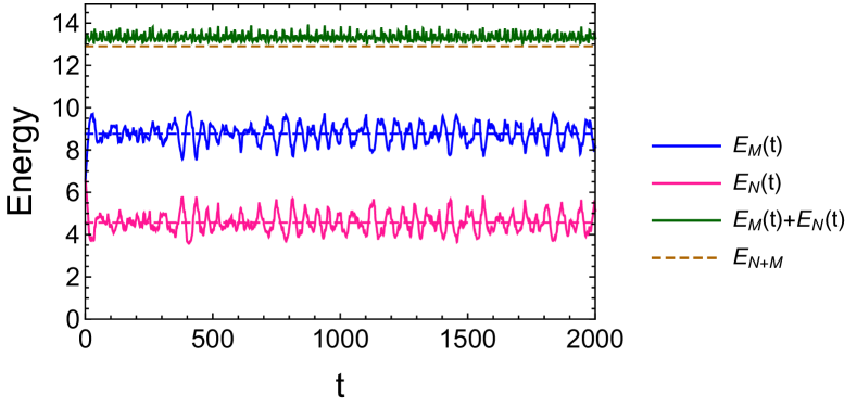
Figure 2: For the initial state $|\psi_{i}\rangle=a^{\dagger}_{3}a^{\dagger}_{4}|0\rangle_{N}\otimes|0\rangle_{M}$ with $N=5$ and $M=10$. $E_{N}(t)$ (in pink) and its long-time average, $E_{M}(t)$ (in blue) and its long time average, the total energy of the state after the quench (in green) and $E_{N}(t)+E_{M}(t)$ (in yellowish green)

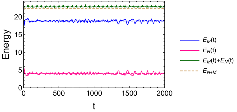
Figure 3: For the initial state $|\psi_{i}\rangle=a^{\dagger}_{3}a^{\dagger}_{4}|0\rangle_{N}\otimes|0\rangle_{M}$ with $N=5$ and $M=25$. $E_{N}(t)$ (in pink) and its long time average , $E_{M}(t)$ (in blue) and its long time average, the total energy of the state after the quench (in green) and $E_{N}(t)+E_{M}(t)$ (in yellowish green)

As we increase the lattice size and the number of excitation modes in the initial state, eigenstates are more delocalized (i.e. smaller IPR)(see 1) in the Hilbert space of the quenched Hamiltonian. As we increase the lattice size — corresponding to increase in delocalization of the initial states — the expectation value of the energy tends towards the long-time average. This is similar to the notion of equilibration in classical systems where two systems at different temperatures in contact, at late times, reach the same temperature. In this case, the two chains are in two different energy eigenstates, however, at late times, both the systems tend to a state with similar average energy per mode (as can be seen in 8 and 9) in the relaxation timescales of the system. In this sense, the equilibration (late time relaxation) is equivalent to the equipartition as well. Equilibration is associated with a late time relaxation to a steady configuration.

To further investigate, let us define,

$$\frac{||\delta E_{M}(t)||}{||\delta E_{M}(0)||}=\frac{||E_{M}(t)-\overline{E_{M}}||}{||E_{M}(0)-\overline{E_{M}}||},$$ (8)

which is the time evolution of the fluctuations of $E_{M}$ about the long time average value of observable $H_{M}$. From 4, 5, 6 and 7, we infer the following:

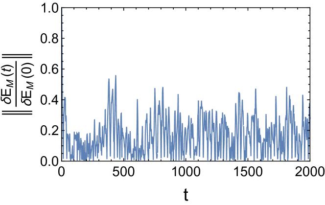
Figure 4: Plot of the fluctuations for initial state $|\psi_{i}\rangle=a^{\dagger}_{3}a^{\dagger}_{4}|0\rangle_{N}\otimes|0\rangle_{M}$ with $N=5$ and $M=10$ for t= [0,2000] for different lattice sizes.

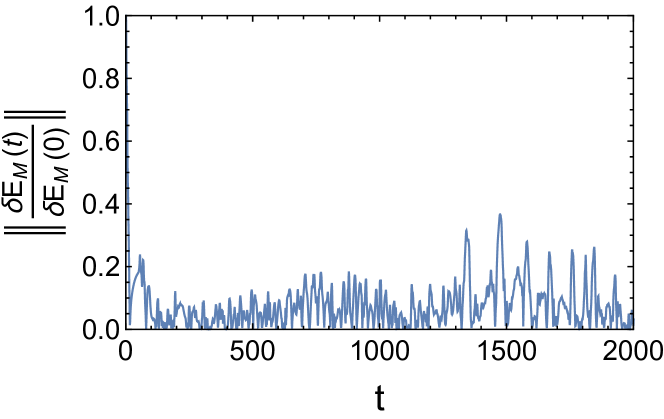
Figure 5: Plot of the fluctuations for initial state $|\psi_{i}\rangle=a^{\dagger}_{3}a^{\dagger}_{4}|0\rangle_{N}\otimes|0\rangle_{M}$ with $N=5$ and $M=25$ for t= [0,2000] for different lattice sizes.

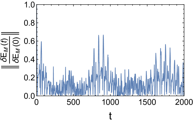
Figure 6: For lattice sizes $N=5$, $M=16$ with initial state $|\psi_{i}\rangle=a^{\dagger}_{3}|0\rangle_{N}\otimes|0\rangle_{M}$. Plot of $\frac{||\delta E_{M}(t)||}{||\delta E_{M}(0)||}$ for t=(0,2000) time steps

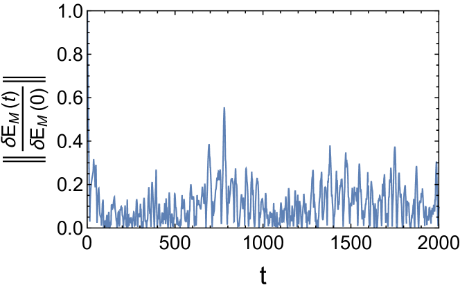
Figure 7: For lattice sizes $N=5$, $M=16$, with initial state $|\psi_{i}\rangle=a^{\dagger}_{3}a^{\dagger}_{4}|0\rangle_{N}\otimes|0\rangle_{M}$. Plot of $\frac{||\delta E_{M}(t)||}{||\delta E_{M}(0)||}$ for t=(0,2000) time steps

The fluctuations remain subdued periodically. As the lattice size increases, this recurrence is rarer. Also for the same lattice, there are smaller fluctuations with farther recurrences for initial states which have better delocalization (See 1). The quasi-periodic nature of observables in finite systems imply that there may be recurrence in long times venuti ; tot , however, the time it takes to relax to a steady state from a non-equilibrium initial condition should be much less than the recurrence timescale of the system. As seen here, the recurrence timescale grow with the system size and it is expected that it grows exponentially with the system size yukalov ; extra . Hence, recurrences become rarer in the thermodynamic limit.

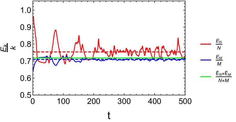
Figure 8: $E_{N}/N$ and $E_{M}/M$ along with their long time averages for t=(0,500) time steps for lattice sizes $N=5$, $M=20$ in initial state $|\psi_{i}\rangle=a^{\dagger}_{3}|0\rangle_{N}\otimes|0\rangle_{M}$

Figure 9: $E_{N}/N$ and $E_{M}/M$ along with their long time averages for t=(0,500) time steps for lattice sizes $N=5$, $M=20$ in initial state $|\psi_{i}\rangle=a^{\dagger}_{3}|0\rangle_{N}\otimes|0\rangle_{M}$

To understand this further and to know whether we can define equilibration between two quantum subsystems, in 8 and 9, we plot the evolution of the average energy per mode for the two subsystems, $E_{N}/N$ and $E_{M}/M$. We observe the following salient features:

• The longtime averages of the observables (per lattice point) relax to GGE expectation value.

• The fluctuations about the average value become smaller with increasing lattice size of the system.

• The per-point observable quantities approach a common value for a specific realization (system size).

IV Analytical Understanding

The numerical evolution of the states clearly indicates that the system relaxes to GGE. However, the numerical analysis does not provide a physical understanding as to (i) why the long time average of the observables relax to GGE? (ii) For what initial conditions, thermalization is violated? and (iii) Is there a way to identify the relation between the delocalization in the Hilbert space and equilibration of states? To go about understanding these issues, we resort to analytical methods and study the observable characteristics of the system at late times.

For the system of Harmonic chains, the normal mode analysis (see Appendix A) makes the study of the system as that of independent oscillators. For this system, prior to the quench, the ground state is a multi-mode Gaussian state. As the quench action is also “quadratic”, the time evolution keeps the state to be Gaussian although the normal modes of the system before and after quench are different. Therefore, the expectation values of any operator can be obtained from the Gaussian density matrix prior to or post quench, with appropriate Bogoliubov coefficients (See Appendix B).

In Appendices C and D, using Bogoliubov transformations, we obtain the evolution and the long time averages of these observables. Using the results in Appendices (B, C and D), we can rewrite the conserved quantities (through the average expectation of the post quench number operator) in terms of the Bogoliubov coefficients as

$$\langle\hat{n^{\prime}}_{k}\rangle=\sum_{l}|\beta_{kl}|^{2}+\sum_{j}\left(|\alpha_{kj}|^{2}n_{j}+|\beta_{kj}|^{2}n_{j}\right).$$ (9)

Physically, the first term in the RHS corresponds to the occupancy when the initial state is vacuum state. This is referred to as vacuum polarization Birrell under the quench. The remaining terms are from the occupancy of the initial states prior to quench, and is referred to as stimulated emission Muller .

Having obtained the results for a general initial state, we can go about understanding the above questions.

First, the periodicity observed in the expectation values directly stem from the beat frequencies of the normal modes. As can be seen from Appendix A, in the thermodynamic limit, the beat frequencies become smaller and the recurrences become rarer. Second, setting the initial state to be ground state, we compute the long-time average of the observables and compare them with the thermal states.

As mentioned earlier, GGE can be used to describe the steady states for integrable systems evolving from a non-equilibrium initial state. With such a description one can generalize the concept of thermalization for integrable systems to relaxation into GGE. We would like to, therefore, compute GGE expectation values of the observables mentioned above and thereby verify the validity of such a description for these states.

GGE is completely described in terms of conserved quantities of the system. Therefore, for our system, we need to find them post quench. The energies (and hence occupation number) of each normal mode in the joint system (after the quench) are conserved as there will be no interactions between these modes and the system is similar to a system of $N+M$ independent harmonic oscillators, with the independent conserved quantities $\hat{n^{\prime}}_{k}=\hat{c}^{\dagger}_{k}\hat{c}_{k},\ k=1,2,\ldots,(N+M)$. Thus, the density matrix of GGE is,

$$\hat{\rho}_{GGE}=\frac{e^{-\sum_{m=1}^{N+M}\lambda_{m}\hat{n^{\prime}}_{m}}}{Tr(e^{-\sum_{m=1}^{N+M}\lambda_{m}\hat{n^{\prime}}_{m}})}$$ (10)

where $\{\lambda_{m}\}$ are Lagrange multipliers.

We can find the Lagrange multipliers, using the initial conditions of the conserved quantities,

$$Tr(\hat{\rho}_{GGE}\hat{n^{\prime}}_{k})=\langle\hat{n^{\prime}}_{k}(0)\rangle$$ (11)

to be

$$\lambda_{k}=\ln\left(\frac{1+\langle\hat{n^{\prime}}_{k}(0)\rangle}{\langle\hat{n^{\prime}}_{k}(0)\rangle}\right)$$ (12)

for $k=1,2\ldots(N+M)$. Therefore, the Lagrange’s multipliers are obtained from the Bogoliubov coefficients. Also, once the state $|\psi_{i}\rangle$ is known in terms of 5, the conserved quantities are known and the Lagrange multipliers are fixed based on the initial state. Vice versa, one can try to obtain the information regarding the initial state through the GGE parameter at late time equilibrium.

This feature is reminiscent of the integrability of the system both pre and post-quench. The late time configuration has to respect the conservation of charges, however, as we will see below if the transformation between the pre quench integrable configuration and post-quench integrable configuration are linearly related aka related through Bogoliubov transformations, the late time conserved charges are totally expressible in terms of early time conserved quantities the state dependency survives for non vacuum initial states Lochan2016 . However, as we can see that with divergent conserved charges $\langle\hat{n^{\prime}}_{k}(0)\rangle$, the appearance of $\lambda$ in the GGE gets weaker.

In a quantum field theoretic generalization Mussardo1 ; *Mussardo2; Doyon:2012bg ; Doyon:2014qsa of the idea of quenching, it will be interesting to see the differentiability of the GGE equilibration with thermalization. Further, in interacting field theories, such differentiability can be dynamically studied 1703.09516 .

Operators $\hat{c}$ and $\hat{c}^{\dagger}$ are traceless matrices in the energy eigenbasis and the trace of a tensor product will be a product of the traces of the individual components. This implies that the correlation matrices $\langle\hat{c}_{i}\hat{c}^{\dagger}_{j}\rangle_{GGE}=\delta_{i,j}\langle\hat{c}_{j}c^{\dagger}_{j}(0)\rangle$ and $\langle c^{\dagger}_{i}c_{j}\rangle_{GGE}=\delta_{i,j}\langle\hat{c}^{\dagger}_{j}\hat{c}_{j}(0)\rangle$ will be diagonal and $\langle\hat{c}_{i}\hat{c}_{j}\rangle_{GGE}=\langle\hat{c}^{\dagger}_{i}\hat{c}^{\dagger}_{j}\rangle_{GGE}=0$. Hence, using this and 11,

$$\langle\hat{n}_{m}(t)\rangle_{GGE}= \frac{4}{(N+M+1)(N+1)}\sum_{i=1}^{N}\sum_{j=1}^{N}\sum_{k=1}^{N+M}\bigg{[}\cosh^{2}(\gamma_{{}_{mk}})\langle\hat{c}^{\dagger}_{k}\hat{c}_{k}(0)\rangle+\sinh^{2}(\gamma_{{}_{mk}})\langle\hat{c}_{k}\hat{c}^{\dagger}_{k}(0)\rangle\bigg{]}$$ (13)

$$\times\sin(\frac{\pi jk}{N+M+1})\sin(\frac{\pi jm}{N+1})\sin(\frac{\pi ik}{N+M+1})\sin(\frac{\pi im}{N+1})$$

$$\langle\hat{n}_{N+m}(t)\rangle_{GGE}= \frac{4}{(N+M+1)(M+1)}\sum_{i=1}^{M}\sum_{j=1}^{M}\sum_{k=1}^{N+M}\bigg{[}\cosh^{2}(\gamma_{{}_{N+m,k}})\langle\hat{c}^{\dagger}_{k}c_{k}(0)\rangle$$ (14)

$$+\sinh^{2}(\gamma_{{}_{N+m,k}})\langle\hat{c}_{k}\hat{c}^{\dagger}_{k}(0)\rangle\bigg{]}\times\sin(\frac{\pi(N+j)k}{N+M+1})$$

$$\times\sin(\frac{\pi jm}{M+1})\sin(\frac{\pi(N+i)k}{N+M+1})\sin(\frac{\pi im}{M+1})$$

Since, $\hat{c}^{\dagger}_{i}\hat{c}_{j}$ (and so $\hat{c}_{i}\hat{c}^{\dagger}_{j}$ ) are conserved quantities and do not evolve in time we can immediately conclude that long time averages computed in Appendix D match the expectation values from the Gibbs Generalized Ensemble.

For thermal states, the evolution in phase space can be described (by virtue of Gaussianity of the density matrix or Wigner function) by the mean and the second moments. Furthermore, the form of the thermal covariance matrix is tightly constrained. Not only it should be diagonal, but the diagonal entries tell us about the Gibbs conserved charges Olivares , that can be used to compare against the numerical relaxation values. The analysis shows that the Gaussian state indeed relaxes to GGE. In Appendix (E), we verify the same using the covariance matrix analysis.

Third, covariance matrix analysis is not sufficient in dealing with non-vacuum energy eigenstates, as these states are not Gaussian. In the case of non-vacuum initial states, as seen from 9, the observables will receive correction over the GGE description. These corrections can be characterized as arising from stimulated emissions. In Appendix (F), we do a detailed analysis on such stimulated emission induced corrections. We observe that for larger lattice size, these corrections are suppressed as $1/N$, where $N$ is the lattice size. In order to verify the description of the system post quench at higher orders of operator expectation, we verify the lattice correlation against its anticipated GGE description in Appendix (G). Further, lower the initial excitation is, smaller is the deviation from GGE. In the thermodynamic limit, the per-point observable quantities get effectively described by GGE (vacuum description), albeit with different values of the parameters in the vacuum state (due to the $N$ dependence). Again, we can identify the generic states which will show significant departures from GGE description. We show that there exists set of well-delocalized states which have the tendency to disobey the GGE description. This behaviour can be understood through divergent conserved charges (in the limit of $\langle\hat{n}^{\prime}_{k}(0)\rangle\to 0)$ which make (some of) the Lagrange multipliers 12 vanish thus letting the description handicapped with the insufficient number of parameters to capture the conservation.

V CONCLUSIONS AND DISCUSSION

While the mechanism and validity of generalized thermalization in integrable systems — where ETH is not valid is still not well understood — many numerical studies have been done with spin systems to verify the validity of the GGE description of their steady states nat ; sys2 ; 1db ; extra . There have been studies investigating whether a sudden change in parameters of the Hamiltonian of an integrable system to another leads to GGE. These studies, however, are mostly done for finite dimensional Hilbert space systems. The harmonic oscillator chain with a finite lattice size, that we have considered, is an infinite dimensional Hilbert space system. So a non-equilibrium initial state can delocalize (i.e. larger IPR values) into infinitely many possible combinations of independent states when we take it into an out of equilibrium condition. Our system also quenches between two integrable configurations in a linear fashion. Therefore, we can utilize the techniques of Bogoliubov transformations for our study. We have investigated the relaxation of eigenstates of such a system.

We have verified the validity of the GGE to describe the long-time average values starting from a non-equilibrium initial state. We also explicitly showed the fluctuations about the steady state with the time evolution of this system. For this system, the longtime averages match the GGE expectation values, yet the fluctuations about this long time average value, although small in the relaxation timescales, are still not negligible.

We were also able to see a form of equilibration between the subsystems for our system. It appears as though the two subsystems are approaching a limit in which the average energy per excitation modes are the same within the relaxation time scales, similar to classical systems. If for a given initial eigenstate, the system indeed evolves to GGE description, the characteristics describing system should be identified and compared against those of GGE. Under general arguments of stimulated emission between integrable systems and thermodynamic limit, we obtained GGE description for finite excitations as well. Using covariance matrix and methods of stimulated emission, we showed that the evolution of the general state (not only eigenstates) to a GGE form in the thermodynamic limit. By corollary, we have obtained the states which may potentially not evolve into a GGE form.

The measure of such states in the Hilbert space is an interesting quantity in order to comment on the generic feature of equilibrium relaxation. The results obtained here can also be attempted for scenarios where the system evolves from one integrable configuration to another post quench, gradually in an asymptotic way, which makes the study interesting from many quantum field theoretic scenarios. We will pursue these issues in a subsequent work.

VI Acknowledgement

Computaions are done using Quantum Package in Mathematica. The authors wish to thank Arul Lakshminarayan, Krishnanand Mallaya and Sandra B for useful discussions. The work is supported under DST-Max Planck Partner Group on Cosmology and Gravity. SM was supported by Inspire fellowship of DST, Government of India. Research of KL is supported by DST-INSPIRE Faculty Fellowship of the Government of India. The authors thank the referees for their constructive suggestions which helped improving the manuscript substantially.

Appendix A The Harmonic chain

A harmonic oscillator chain is a well known integrable system. With periodic boundary conditions, this Hamiltonian in the thermodynamic limit would correspond to a free field theory. The Hamiltonian of a N body harmonic oscillator lattice with nearest neighbor interactions can be written as,

$$H=\sum_{i=1}^{N}\frac{p_{i}^{2}}{2m}+\frac{1}{2}m\omega_{0}^{2}(q_{i+1}-q_{i})^{2}$$ (15)

where $\omega_{0}$ is the natural frequency of the individual oscillator, $p_{i}$ and $q_{i}$ are the respective momentum and position coordinates for a harmonic oscillator on the $i^{th}$ lattice site with a lattice distance of $a$. In this work we use static boundary conditions, which means $q_{1}=q_{N+1}=0$. For large $N$, the results are independent of the choice of the boundary condition.

Rewriting the Hamiltonian in terms of the normal modes leads to a system of N uncoupled harmonic oscillators:

$$\hat{H}=\sum_{k=1}^{N}\hbar\ \omega_{k}(\hat{a}^{\dagger}_{k}\hat{a}_{k}+\frac{1}{2})$$ (16)

where $\hat{a}^{\dagger}_{k}$ and $\hat{a}_{k}$ are the creation and annihilation operators with normal mode frequencies,

$$\omega_{k}=2\omega_{0}\left|\sin\left(\frac{\pi k}{2(N+1)}\right)\right|.$$ (17)

As we will explicitly calculate in other sections of the appendix, the beat frequencies appearing in the various expectations are determined by

$$\left|\omega_{k}-\omega_{j}\right| = 2\omega_{0}\left|\sin\left(\frac{\pi k}{2(N+1)}\right)-\sin\left(\frac{\pi j}{2(N+1)}\right)\right|$$ (18)

$$= 4\omega_{0}\left|\sin\left(\frac{\pi(k-j)}{2(N+1)}\right)\cos\left(\frac{\pi(k+j)}{2(N+1)}\right)\right|.$$

The $(k-j)$ takes values $N+1-m$ with $m\in 2,3,..$. Therefore, in the thermodynamic limit, most of the beat frequencies become smaller and therefore the recurrences occur lately. For smaller lattice sizes, two normal mode frequencies can easily be separate enough to show periodicity effectively, while for the larger systems, the probability of finding separate enough normal modes will be rarer, hence the oscillatory terms get suppressed in overall contribution.

Appendix B Bogoliubov Transformations

As mentioned earlier, the normal modes of the system before and after the quench are different. In order to obtain the relation between the creation and annihilation operators before and after the quench, we need to diagonalize the Hamiltonian by applying the Bogoliubov transformations. Using the definitions for normal mode coordinates before and after the quench ($Q_{k}$ and $Q^{\prime}_{k}$ respectively), we have,

$$Q_{l} = \sqrt{\frac{2}{N+1}}\sum_{m=1}^{N}q_{m}\sin\left(\frac{\pi lm}{N+1}\right)=\sqrt{\frac{4}{(N+1)(N+M+1)}}$$ (19)

$$\times \sum_{m=1}^{N}\sum_{k=1}^{N+M}Q^{\prime}_{k}\sin\left(\frac{\pi mk}{N+M+1}\right)\sin\left(\frac{\pi lm}{N+1}\right),$$

where $q_{k}$ is real space variable. We can use the relationship of the creation and annihilation operators before and after the quench to get,

$$\hat{a}_{l}+\hat{a}^{\dagger}_{l} = \sqrt{\frac{2}{N+1}}\sqrt{\frac{2}{N+M+1}}\sum_{m=1}^{N}\sum_{k=1}^{N+M}$$

$$\times e^{\gamma_{{}_{l,k}}}(\hat{c}_{k}+\hat{c}^{\dagger}_{k})\sin\left(\frac{\pi mk}{N+M+1}\right)\sin\left(\frac{\pi lm}{N+1}\right)$$

where $e^{\gamma_{{}_{l,k}}}=\sqrt{\frac{\omega_{l}}{\omega^{\prime}_{k}}}$.

Similarly we can use $P^{\prime}_{l}$ to get an expression for $\hat{a}_{l}-\hat{a}^{\dagger}_{l}$ and adding these to expressions lead to:

$$\hat{a}_{l}=\sqrt{\frac{2}{N+1}}\sqrt{\frac{2}{N+M+1}}\sum_{m=1}^{N}\sum_{k=1}^{N+M}\left(\cosh(\gamma_{{}_{l,k}})\hat{c}_{k}+\sinh(\gamma_{{}_{l,k}})\hat{c}^{\dagger}_{k}\right)\sin\left(\frac{\pi mk}{N+M+1}\right)\sin\left(\frac{\pi lm}{N+1}\right)$$ (21)

The Hermitian conjugate of 21 lead to the expansion for $\hat{a}^{\dagger}_{l}$. Similarly for $\hat{a}_{N+l}$ we get,

$$\hat{a}_{N+l}=\sqrt{\frac{2}{M+1}}\sqrt{\frac{2}{N+M+1}}\sum_{i=1}^{M}\sum_{k=1}^{N+M}\left(\cosh(\gamma_{{}_{N+l,k}})\hat{c}_{k}+\sinh(\gamma_{{}_{N+l,k}})\hat{c}^{\dagger}_{k}\right)\sin\left(\frac{\pi(N+i)k}{N+M+1}\right)\sin\left(\frac{\pi li}{M+1}\right)$$ (22)

Thus, we obtain the Bogoliubov transformations that relate the creation and annihilation operators of the system before and after the quench as

$$\alpha_{lk} = \sqrt{\frac{2}{N+1}}\sqrt{\frac{2}{N+M+1}}\sum_{m=1}^{N}\cosh(\gamma_{{}_{l,k}})\sin\left(\frac{\pi mk}{N+M+1}\right)\sin\left(\frac{\pi lm}{N+1}\right),$$ (23)

$$\beta_{lk} = \sqrt{\frac{2}{N+1}}\sqrt{\frac{2}{N+M+1}}\sum_{m=1}^{N}\sinh(\gamma_{{}_{l,k}})\sin\left(\frac{\pi mk}{N+M+1}\right)\sin\left(\frac{\pi lm}{N+1}\right)$$ (24)

for $l:1\rightarrow N$, and

$$\alpha_{lk} = \sqrt{\frac{2}{M+1}}\sqrt{\frac{2}{N+M+1}}\sum_{i=1}^{M}\cosh(\gamma_{{}_{N+l,k}})\sin\left(\frac{\pi(N+i)k}{N+M+1}\right)\sin\left(\frac{\pi li}{M+1}\right),$$ (25)

$$\beta_{lk} = \sqrt{\frac{2}{M+1}}\sqrt{\frac{2}{N+M+1}}\sum_{i=1}^{M}\sinh(\gamma_{{}_{N+l,k}})\sin\left(\frac{\pi(N+i)k}{N+M+1}\right)\sin\left(\frac{\pi li}{M+1}\right),$$ (26)

for $l:N+1\rightarrow N+M$. The transformations 19 can similarly be inverted to obtain the inverse Bogoliubov coefficients $\tilde{\alpha}_{lk},\tilde{\beta}_{lk}$, which by the property of real, symmetric, orthogonal transformation between real space and normal mode, are easy to compute.

Appendix C Observables

To study equilibrium relaxation in this system we consider some observables to probe the system. In this case, we use the occupation number of the modes of the disjoint system, i. e.,

$$\hat{n}_{m}=\hat{a}^{\dagger}_{m}\hat{a}_{m},\ m=1,2\ldots,(N+M)$$ (27)

Since these operators do not commute with the Hamiltonian ($\hat{H}$) after the quench, the time evolution is expected to be non-trivial. Using the Bogoliubov transformations and the evolution properties of $\hat{c}^{\dagger}$ and $\hat{c}$ operators, the time evolution of the occupation numbers is given by,

$$\langle\hat{n}_{m}(t)\rangle= \frac{4}{(N+M+1)(N+1)}\sum_{i,j=1}^{N}\sum_{k,l=1}^{N+M}\bigg{[}\cosh\gamma_{{}_{m,k}}\,\cosh\gamma_{{}_{m,l}}e^{\frac{i(\omega^{\prime}_{l}-\omega^{\prime}_{k})t}{\hbar}}\langle\hat{c}^{\dagger}_{l}\hat{c}_{k}\rangle+\sinh\gamma_{{}_{m,k}}\cosh\gamma_{{}_{m,l}}e^{\frac{i(\omega^{\prime}_{l}+\omega^{\prime}_{k})t}{\hbar}}\langle\hat{c}^{\dagger}_{l}\hat{c}^{\dagger}_{k}\rangle$$ (28)

$$+\cosh\gamma_{{}_{m,k}}\sinh\gamma_{{}_{m,l}}\,e^{\frac{i(-\omega^{\prime}_{l}-\omega^{\prime}_{k})t}{\hbar}}\langle\hat{c}_{l}\hat{c}_{k}\rangle$$

$$+\sinh\gamma_{{}_{m,k}}\sinh\gamma_{{}_{m,l}}e^{\frac{i(-\omega^{\prime}_{l}-\omega^{\prime}_{k})t}{\hbar}}\langle\hat{c}_{l}\hat{c}^{\dagger}_{k}\rangle\bigg{]}\sin(\frac{\pi jl}{N+M+1})\sin(\frac{\pi jm}{N+1})\sin(\frac{\pi ik}{N+M+1})\sin(\frac{\pi im}{N+1})$$

for $m:1\rightarrow N$, and

$$\langle\hat{n}_{N+m}(t)\rangle= \frac{4}{(N+M+1)(M+1)}\sum_{i=1}^{M}\sum_{j=1}^{M}\sum_{k=1}^{N+M}\sum_{l=1}^{N+M}\bigg{[}\cosh(\gamma_{{}_{N+m,k}})\cosh(\gamma_{{}_{N+m,l}})e^{\frac{i(\omega^{\prime}_{l}-\omega^{\prime}_{k})t}{\hbar}}\langle\hat{c}^{\dagger}_{l}\hat{c}_{k}\rangle$$ (29)

$$+\sinh(\gamma_{{}_{N+m,k}})\cosh(\gamma_{{}_{N+m,l}})e^{\frac{i(\omega^{\prime}_{l}+\omega^{\prime}_{k})t}{\hbar}}\langle\hat{c}^{\dagger}_{l}\hat{c}^{\dagger}_{k}\rangle+\cosh(\gamma_{{}_{N+m,k}})\sinh(\gamma_{{}_{N+m,l}})e^{\frac{i(-\omega^{\prime}_{l}-\omega^{\prime}_{k})t}{\hbar}}\langle\hat{c}_{l}\hat{c}_{k}\rangle$$

$$+\sinh(\gamma_{{}_{N+m,k}})\sinh(\gamma_{{}_{N+m,l}})e^{\frac{i(-\omega^{\prime}_{l}-\omega^{\prime}_{k})t}{\hbar}}\langle\hat{c}_{l}\hat{c}^{\dagger}_{k}\rangle\bigg{]}\times\sin(\frac{\pi(N+j)l}{N+M+1}\times\sin(\frac{\pi jm}{M+1})\sin(\frac{\pi(N+i)k}{N+M+1})\sin(\frac{\pi im}{M+1})$$

for $m:1\rightarrow M$. In order to evaluate the quantum expectation of the number operator at any instant of time $t$, we need to obtain the correlation matrices $\langle\hat{c}^{\dagger}_{i}\hat{c}^{\dagger}_{j}\rangle$,$\langle\hat{c}_{i}\hat{c}^{\dagger}_{j}\rangle$, $\langle\hat{c}^{\dagger}_{i}\hat{c}_{j}\rangle$ and $\langle\hat{c}_{i}\hat{c}_{j}\rangle$.

Once we obtain the average occupation numbers, it possible to obtain the evolution of the energies of the disjoint modes as, $\langle\hat{H}_{N}(t)\rangle=E_{N}(t)=\sum_{i=1}^{N}(\hat{n}_{i}(t)+1/2)\hbar\omega_{i}$ and $\langle\hat{H}_{M}(t)\rangle=E_{M}(t)=\sum_{i=1}^{M}(\hat{n}_{N+i}(t)+1/2)\hbar\omega_{N+i}$ using the occupation numbers we have computed above.

Appendix D Long time averages

From 28 and 29, it is easy to see that that the long time average will include only the diagonal elements as only for the those values will the exponential factor vanish.

Hence, the long time average of the expectation value of the number operator is given by

$$\overline{\langle\hat{n}_{m}(t)}\rangle= \frac{4}{(N+M+1)(N+1)}\sum_{i=1}^{N}\sum_{j=1}^{N}\sum_{k=1}^{N+M}\bigg{[}\cosh^{2}(\gamma_{{}_{mk}})\langle\hat{c}^{\dagger}_{k}\hat{c}_{k}\rangle+\sinh^{2}(\gamma_{{}_{mk}})\langle\hat{c}_{k}\hat{c}^{\dagger}_{k}\rangle\bigg{]}$$ (30)

$$\times\sin(\frac{\pi jk}{N+M+1})\sin(\frac{\pi jm}{N+1})\sin(\frac{\pi ik}{N+M+1})\sin(\frac{\pi im}{N+1})$$

for $m:1\rightarrow N$, and

$$\overline{\langle\hat{n}_{N+m}(t)}\rangle= \frac{4}{(N+M+1)(M+1)}\sum_{i=1}^{M}\sum_{j=1}^{M}\sum_{k=1}^{N+M}\bigg{[}\cosh^{2}(\gamma_{{}_{N+m,k}})\langle\hat{c}^{\dagger}_{k}\hat{c}_{k}\rangle+\sinh^{2}(\gamma_{{}_{N+m,k}})\langle\hat{c}_{k}\hat{c}^{\dagger}_{k}\rangle\bigg{]}$$ (31)

$$\times\sin(\frac{\pi(N+j)k}{N+M+1})\sin(\frac{\pi jm}{M+1})\sin(\frac{\pi(N+i)k}{N+M+1})\sin(\frac{\pi im}{M+1})$$

for $m:1\rightarrow M$.

Appendix E Covariance Matrix

For Gaussian states, the information is encoded in the second moment which is also encoded in the covariance matrix in the phase space. Structurally, the covariance matrix is given as

$$\sigma_{NM}=\left(\begin{array}[]{ll}\sigma_{xx}&\sigma_{xp}\\ \sigma_{xp}&\sigma_{pp}\end{array}\right)$$ (34)

The covariance matrix before the quench, in the normal modes of the ‘non-quenched’ Hamiltonian, is given as

$$\sigma_{NM}=\left(\begin{array}[]{llllll}a_{11}&..&a_{1n}&b_{11}&..&b_{1n}\\ ..&..&..&..&..&..\\ a_{n1}&..&a_{nn}&b_{n1}&..&b_{nn}\\ b_{11}&..&b_{1n}&\tilde{a}_{11}&..&\tilde{a}_{1n}\\ ..&..&..&..&..&..\\ b_{n1}&..&b_{nn}&\tilde{a}_{n1}&..&\tilde{a}_{nn}\end{array}\right)$$ (41)

If we go to the phase space corresponding to the configuration space variables of the system, the covariance matrix becomes

$$\sigma=S^{T}\sigma_{NM}S,$$ (42)

where $S$ is given by

$$S=\left(\begin{array}[]{llll}S_{N}&0&0&0\\ 0&S_{M}&0&0\\ 0&0&S_{N}&0\\ 0&0&0&S_{M}\\ \end{array}\right)$$ (47)

which is a similarity transformation from the configuration space to the normal modes and

$$S_{K}=\sqrt{\frac{2}{K+1}}\left(\begin{array}[]{lll}\sin{\frac{\pi}{K+1}}&..&\sin{\frac{K\pi}{K+1}}\\ ..&..&..\\ \sin{\frac{K\pi}{K+1}}&..&\sin{\frac{K^{2}\pi}{K+1}}\\ \end{array}\right).$$ (51)

$K$ takes values $N,M$. Clearly, being a symmetric orthogonal matrix $S$ is its inverse as well. Since it is easier to go to the normal modes of quenched system from the configuration space we cast the covariance matrix in the configuration space through 42.

Post quenching, the system can be expressed in terms of normal modes of the quenched system and we cast the covariance matrix in the new normal mode basis of the quenched system to study its time evolution. The recasting in the normal mode basis is done again by an orthogonal transformation

$$\tilde{S}_{N+M}=\sqrt{\frac{2}{N+M+1}}\left(\begin{array}[]{llllll}\sin{\frac{\pi}{N+M+1}}&..&\sin{\frac{(N+M)\pi}{N+M+1}}&0&..&0\\ ..&..&..&..&..&..\\ \sin{\frac{(N+M)\pi}{N+M+1}}&..&\sin{\frac{(N+M)^{2}\pi}{N+M+1}}&0&..&0\\ 0&..&0&\sin{\frac{\pi}{N+M+1}}&..&\sin{\frac{(N+M)\pi}{N+M+1}}\\ ..&..&..&..&..&..\\ 0&..&0&\sin{\frac{(N+M)\pi}{N+M+1}}&..&\sin{\frac{(N+M)^{2}\pi}{N+M+1}}\end{array}\right).$$ (58)

Therefore, the covariance matrix post quenching is given as

$$\sigma_{PQ}=\tilde{S}_{N+M}(S^{T}\sigma_{NM}S)\tilde{S}_{N+M}^{T}.$$ (59)

Let us call

$$\sigma_{PQ}=\left(\begin{array}[]{llllll}a^{\prime}_{11}&..&a^{\prime}_{1n}&b^{\prime}_{11}&..&b^{\prime}_{1n}\\ ..&..&..&..&..&..\\ a^{\prime}_{n1}&..&a^{\prime}_{nn}&b^{\prime}_{n1}&..&b^{\prime}_{nn}\\ b^{\prime}_{11}&..&b^{\prime}_{1n}&\tilde{a}^{\prime}_{11}&..&\tilde{a}^{\prime}_{1n}\\ ..&..&..&..&..&..\\ b^{\prime}_{n1}&..&b^{\prime}_{nn}&\tilde{a}^{\prime}_{n1}&..&\tilde{a}^{\prime}_{nn}\end{array}\right).$$ (66)

Further, in the normal modes basis, we have $N+M$ decoupled harmonic oscillators whose time evolution is obtained as a transformation given by matrix

$$U_{t}=\left(\begin{array}[]{llllll}\cos{\omega_{1}t}&..&0&\frac{\sin{\omega_{1}t}}{\omega_{1}}&..&0\\ ..&..&..&..&..&..\\ 0&..&\cos{\omega_{{}_{N+M}}t}&0&..&\frac{\sin{\omega_{{}_{N+M}}t}}{\omega_{{}_{N+M}}}\\ -\omega_{1}\sin{\omega_{1}t}&..&0&\cos{\omega_{1}t}&..&0\\ ..&..&..&..&..&..\\ 0&..&-\omega_{{}_{N+M}}\sin{\omega_{{}_{N+M}}t}&0&..&\cos{\omega_{{}_{N+M}}t}\\ \end{array}\right),$$ (73)

It is important to note that this is not unitary in the phase space. Thus the time evolution drives the covariance matrix to

$$\sigma_{PQ}(t)=U_{t}^{T}\sigma_{PQ}U_{t}=\chi^{T}\sigma_{NM}\chi,$$ (74)

with

$$\chi=S\tilde{S}_{N+M}^{T}U_{t}.$$ (75)

The generic form of the off-diagonal terms in the covariance matrix post quench are given as

$$(\sigma_{PQ;xx})_{ij} = a^{\prime}_{ij}\cos{\omega_{j}t}\cos{\omega_{i}t}-b^{\prime}_{ij}\omega_{j}\sin{\omega_{j}t}\cos{\omega_{i}t}-b^{\prime}_{ij}\omega_{i}\cos{\omega_{j}t}\sin{\omega_{i}t}+\tilde{a}^{\prime}_{ij}\omega_{i}\omega_{j}\sin{\omega_{j}t}\sin{\omega_{i}t}$$

$$(\sigma_{PQ;xp})_{ij} = \omega_{j}^{-1}a^{\prime}_{ij}\sin{\omega_{j}t}\cos{\omega_{i}t}+b^{\prime}_{ij}\cos{\omega_{i}t}\cos{\omega_{j}t}-\frac{\omega_{i}}{\omega_{j}}b^{\prime}_{ij}\sin{\omega_{i}t}\sin{\omega_{j}t}-\tilde{a}^{\prime}_{ij}\omega_{i}\sin{\omega_{i}t}\cos{\omega_{j}t}.$$ (76)

For the vacuum state, evidently $a_{ij}|_{i\neq j}=0,b_{ij}=0\Rightarrow b^{\prime}_{ij}=0$. Therefore, the off-diagonal elements of the quenched covariance matrix become purely oscillatory in nature. The long-time averages over such covariance matrices can be effectively replaced by a diagonal Gaussian covariance matrix, which acquire GGE form. The diagonal elements, obtained from 59 and 66, give the occupancy across different modes, which is exactly the first term on the RHS of 9. Similar exercise for any pre-quenching initial eigenstate reproduces 9.

Appendix F Fate of a general Fock basis state under quench

As discussed previously, any non-vacuum eigenstates will bring corrections as depicted in 9. If the initial state is taken to be an eigenstate of the pre-quenched Hamiltonian, i.e.

$$|\Psi_{in}\rangle=|n_{1},n_{2},...\rangle_{M}\otimes|n_{N+1},n_{N+2},..\rangle_{N}$$ (77)

the off diagonal parts of the initial covariance matrix are given as (by writing the individual $x_{i}$ and $p_{j}$’s in terms of the creation and annihilation operators)

$$\sigma_{x_{i}x_{j}} = \langle\Psi|\frac{\hat{x}_{i}\hat{x}_{j}+\hat{x}_{j}\hat{x}_{i}}{2}|\Psi\rangle\big{|}_{i\neq j}=0,$$ (78)

$$\sigma_{x_{i}p_{j}} = \langle\Psi|\frac{\hat{x}_{i}\hat{p}_{j}+\hat{p}_{j}\hat{x}_{i}}{2}|\Psi\rangle=0.$$ (79)

owing to $b_{ij}=0$ in 76 for the energy eigenstates 77. We note the following points: The initial states, for which $b_{ij}=0$, the long time average of the covariance matrix will lead to thermal form. Clearly these states satisfy the necessary criterion of a diagonal covariance matrix. It is also evident from the oscillatory behaviour of the $b^{\prime}_{ij}$ that for any initial finite $b_{ij}$ the late time $b^{\prime}_{ij}\rightarrow 0$. However, for the initial states, which have $b_{ij}\nless\infty$ may potentially violate thermalization. A simple example of such states in the Hilbert space may be the class of separable states of the kind

$$|\Psi\rangle=\sum_{n_{1},n_{2},..,n_{M},..n_{N+M}}\!\!\!\!\!\!\!\!\!\!\!\!\!\!\!c_{n_{1}}....c_{n_{N+M}}|n_{1}..n_{M},...n_{N+M}\rangle,$$ (80)

where for at least one $c_{n_{m}},$ we should have $|c_{n_{m}}|^{2}\sim\frac{1}{(n_{m})^{1/2-\epsilon}}$, at least for $n_{m}\gg 1$. This condition is sufficient to ensure the normalization of the state, however, for such states $\langle x_{m}\rangle=\sum_{n_{m}}c_{n_{m}}(\sqrt{n_{m}}c^{*}_{n_{m}-1}+\sqrt{n_{m}+1}c^{*}_{n_{m}+1})\rightarrow\infty$. Therefore, the late time $b^{\prime}_{ij}$ in the covariance matrix can still survive, forbidding the system to land up in a GGE configuration. Such states may well be very delocalized as we just require one of the $c_{n_{m}}$ to have the above mentioned property. Therefore a fine distribution of over various energy eigenstates is permissible rendering localization inefficient. These states have the property that some of the conserved charges are divergent, for which already failure of GGE has been argued Kormos . Such states are highly energetic ones, but definitely physical, as they belong to square integrable class. The analysis of measure of such states in the Hilbert space is an interesting topic, which we will pursue in a subsequent work. These kind of states may also be relevant in the case of black hole physics, where non-thermality of the configuration may be related to memory of the in- state, while the energetics of such states may shed some light on the firewall proposal Almheiri .

Coming back to the eigenstates, the comparison of the diagonal elements of the time averaged covariance matrix expectedly recovers 13,14, which supports the GGE description. We now further probe the excited eigenstates with their long time average expectation values.

Clearly, in the free harmonic oscillator system, all observables are described by the correlators $\langle\hat{c}_{k}(t)\hat{c}^{\dagger}_{k^{\prime}}(t)\rangle$. As discussed in the previous appendices, the long time average for any observable will be solely determined by $\langle\hat{c}_{k}(0)\hat{c}^{\dagger}_{k}(0)\rangle$. Therefore, we can use 9 for determining such quantities per unit lattice. Clearly, for initial excited states, the Gaussian (GGE) description will be corrected. The deviation from such a description is characterized by

$$\Delta_{G}=\frac{\sum_{j}\left(|\tilde{\alpha}_{kj}|^{2}n_{j}+|\tilde{\beta}_{kj}|^{2}n_{j}\right)/N}{\sum_{l}|\tilde{\beta}_{kl}|^{2}/N}$$ (81)

In the limit $N\rightarrow\infty$,

$$\Delta_{G} \rightarrow {\cal O}\left(\frac{\sum_{j}n_{j}}{N}\right).$$ (82)

Therefore, in the thermodynamic limit, for any finitely excited state (sub-part of the full system) the effective description is essentially GGE. Also, we note that quantum states for which $\Delta_{G}\sim{\cal O}\left(1\right)$ will not relax to a generalized thermal setting effectively.

Appendix G Correlation between the lattice sites

In order to check the effectiveness of GGE relaxation, we explore the correlation between different lattice sites, post quenching. Therefore, the operator to explore would be

$$\langle\psi|\hat{n}_{k_{1}}^{\prime}\hat{n}_{k_{2}}^{\prime}|\psi\rangle={}_{M}\langle 0|{}_{N}\langle 0|\hat{c}_{k_{1}}^{\dagger}\hat{c}_{k_{1}}\hat{c}_{k_{2}}^{\dagger}\hat{c}_{k_{2}}|0\rangle_{M}|0\rangle_{N},$$ (83)

which measures the correlation between $k_{1}-$th and $k_{2}-$th site. Writing

$$\hat{c}_{k}=\sum_{k^{\prime}}\tilde{\alpha}_{kk^{\prime}}\hat{a}_{k^{\prime}}+\tilde{\beta}_{kk^{\prime}}\hat{a}_{k}^{\dagger},$$ (84)

we obtain,

$$\langle\psi|\hat{n}_{k_{1}}^{\prime}\hat{n}_{k_{2}}^{\prime}|\psi\rangle=\sum_{lm}\left(\tilde{\beta}_{k_{1}l}\tilde{\beta}_{k_{2}m}^{*}\tilde{\alpha}_{k_{1}m}\tilde{\alpha}_{k_{2}l}^{*}+\tilde{\beta}_{k_{1}l}\tilde{\beta}_{k_{2}l}^{*}\tilde{\alpha}_{k_{1}m}\tilde{\alpha}_{k_{2}m}^{*}+|\tilde{\beta}_{k_{1}l}\tilde{\beta}_{k_{2}m}|^{2}\right)\,.$$ (85)

Owing to the real character of the Bogoliubov coefficients along with 24, 26 and the relation (for the Bogoliubov coefficients to yield the correct commutation relations)

$$\sum_{k^{\prime}}\tilde{\alpha}_{kk^{\prime}}\tilde{\beta}_{lk^{\prime}}-\tilde{\alpha}_{lk^{\prime}}\tilde{\beta}_{kk^{\prime}}=0,$$ (86)

we obtain in that the first two terms in the RHS of 85 are measure to the ($Q_{k_{1}}Q_{k_{2}}$, $Q_{k_{1}}P_{k_{2}}$, etc.) correlations post quench, which vanish. Therefore, only the third term survives and we have

$$\langle\psi|\hat{n}_{k_{1}}^{\prime}\hat{n}_{k_{2}}^{\prime}|\psi\rangle=\sum_{lm}|\tilde{\beta}_{k_{1}l}\tilde{\beta}_{k_{2}m}|^{2}=\langle n_{k_{1}}^{\prime}\rangle\langle n_{k_{2}}^{\prime}\rangle,$$ (87)

which is obtained for the initial vacuum state pre quenching, i.e. $n_{i}=0,\hskip 2.84544pt\forall i$ in 9. Therefore, post quench the system lands up in a configuration in which there is no real quantum correlation between different lattice sites, as suited for a Gibbs Generalized ensemble. If the density matrix description of this state post quench is indeed that of a Gibbs Generalized Ensemble, then the two point correlation can be obtained as

$$\langle\hat{n}_{k_{1}}^{\prime}\hat{n}_{k_{2}}^{\prime}\rangle=\frac{Tr[n_{k_{1}}^{\prime}n_{k_{2}}^{\prime}\rho_{GGE}]}{Tr[\rho_{GGE}]}.$$ (88)

Since $n_{K}$s are conserved charges of the system post quench,

$$\rho_{GGE}=e^{-\sum_{k}\lambda_{k}n_{k}^{\prime}}.$$ (89)

A simple computation yields,

$$\langle\hat{n}_{k_{1}}^{\prime}\hat{n}_{k_{2}}^{\prime}\rangle=\frac{e^{-\lambda_{k_{1}}}}{(1-e^{-\lambda_{k_{1}}})}\frac{e^{-\lambda_{k_{2}}}}{(1-e^{-\lambda_{k_{2}}})}.$$ (90)

Since previously we obtained,

$$e^{\lambda_{k}}=1+\frac{1}{\langle n_{k}(0)^{\prime}\rangle},$$ (91)

we finally have,

$$\langle\hat{n}_{k_{1}}^{\prime}\hat{n}_{k_{2}}^{\prime}\rangle=\langle n_{k_{1}}^{\prime}\rangle\langle n_{k_{2}}^{\prime}\rangle,$$ (92)

relating the two-point correlation post quench to that of classical correlation i.e.

$$\langle n_{k_{1}}^{\prime}n_{k_{2}}^{\prime}\rangle-\langle n_{k_{1}}^{\prime}\rangle\langle n_{k_{2}}^{\prime}\rangle=0,$$

as in 87.

References

- (1) P. P. V. McClintock, Contemporary Physics 51, 186 (2010)
- (2) C. Gogolin and J. Eisert, Reports on Progress in Physics 79, 056001 (May 2016), arXiv:1503.07538 [quant-ph]
- (3) M. Gring, M. Kuhnert, T. Langen, T. Kitagawa, B. Rauer, M. Schreitl, I. Mazets, D. A. Smith, E. Demler, and J. Schmiedmayer, Science 337, 1318 (2012), ISSN 0036-8075
- (4) A. Polkovnikov, K. Sengupta, A. Silva, and M. Vengalattore, Rev. Mod. Phys. 83, 863 (Aug 2011), https://link.aps.org/doi/10.1103/RevModPhys.83.863
- (5) J. von Neumann, The European Physical Journal H 35, 201 (Nov 2010), ISSN 2102-6467, https://doi.org/10.1140/epjh/e2010-00008-5
- (6) J. M. Deutsch, Phys. Rev. A 43, 2046 (Feb 1991), http://link.aps.org/doi/10.1103/PhysRevA.43.2046
- (7) M. Srednicki, Physical Review E 50, 888 (1994)
- (8) M. Rigol and M. Srednicki, Phys. Rev. Lett. 108, 110601 (Mar 2012), ISSN 00319007, arXiv:1108.0928, http://link.aps.org/doi/10.1103/PhysRevLett.108.110601
- (9) T. Langen, R. Geiger, and J. Schmiedmayer, Annual Review of Condensed Matter Physics 6, 201 (2015), https://doi.org/10.1146/annurev-conmatphys-031214-014548, https://doi.org/10.1146/annurev-conmatphys-031214-014548
-
(10)
M. Rigol, V. Dunjko, and M. Olshanii, Nature 452, 854 (04 2008), http://dx.doi.org/10.1038/nature06838.
Key: nat
Annotation: 10.1038/nature06838. - (11) M. Rigol, V. Dunjko, V. Yurovsky, and M. Olshanii, Phys. Rev. Lett. 98, 050405 (Feb 2007), http://link.aps.org/doi/10.1103/PhysRevLett.98.050405
- (12) L. D. Alessioa, Y. Kafric, A. Polkovnikov, and M. Rigol, arXiv:1509.06411(2015)
- (13) A. C. Cassidy, C. W. Clark, and M. Rigol, Phys. Rev. Lett. 106, 140405 (Apr 2011), http://link.aps.org/doi/10.1103/PhysRevLett.106.140405
- (14) A. Iucci and M. A. Cazalilla, Phys. Rev. A 80, 063619 (Dec 2009), https://link.aps.org/doi/10.1103/PhysRevA.80.063619
- (15) X.-W. Guan, M. T. Batchelor, and C. Lee, Rev. Mod. Phys. 85, 1633 (Nov 2013), https://link.aps.org/doi/10.1103/RevModPhys.85.1633
- (16) F. H. L. Essler and M. Fagotti, Journal of Statistical Mechanics: Theory and Experiment 2016, 064002 (2016), http://stacks.iop.org/1742-5468/2016/i=6/a=064002
- (17) L. Vidmar and M. Rigol, Journal of Statistical Mechanics: Theory and Experiment 2016, 064007 (2016), http://stacks.iop.org/1742-5468/2016/i=6/a=064007
- (18) B. Pozsgay, Journal of Statistical Mechanics: Theory and Experiment 2013, P07003 (2013), http://stacks.iop.org/1742-5468/2013/i=07/a=P07003
- (19) M. Fagotti and F. H. L. Essler, Journal of Statistical Mechanics: Theory and Experiment 2013, P07012 (2013), http://stacks.iop.org/1742-5468/2013/i=07/a=P07012
- (20) M. Fagotti, M. Collura, F. H. L. Essler, and P. Calabrese, Phys. Rev. B 89, 125101 (Mar 2014), https://link.aps.org/doi/10.1103/PhysRevB.89.125101
- (21) B. Pozsgay, M. Mestyán, M. A. Werner, M. Kormos, G. Zaránd, and G. Takács, Phys. Rev. Lett. 113, 117203 (Sep 2014), https://link.aps.org/doi/10.1103/PhysRevLett.113.117203
- (22) K. K. Kozlowski and B. Pozsgay, Journal of Statistical Mechanics: Theory and Experiment 2012, P05021 (2012), http://stacks.iop.org/1742-5468/2012/i=05/a=P05021
- (23) A. De Luca, M. Collura, and J. De Nardis, Phys. Rev. B 96, 020403 (Jul 2017), https://link.aps.org/doi/10.1103/PhysRevB.96.020403
- (24) W. H. Aschbacher and C.-A. Pillet, Journal of Statistical Physics 112, 1153 (Sep 2003), ISSN 1572-9613, https://doi.org/10.1023/A:1024619726273
- (25) W. H. Aschbacher and J.-M. Barbaroux, Letters in Mathematical Physics 77, 11 (Jul 2006), ISSN 1573-0530, https://doi.org/10.1007/s11005-006-0049-7
- (26) A. De Luca, G. Martelloni, and J. Viti, Phys. Rev. A 91, 021603 (Feb 2015), https://link.aps.org/doi/10.1103/PhysRevA.91.021603
- (27) M. Rigol, A. Muramatsu, and M. Olshanii, Phys. Rev. A 74, 053616 (Nov 2006), https://link.aps.org/doi/10.1103/PhysRevA.74.053616
- (28) T. Caneva, E. Canovi, D. Rossini, G. E. Santoro, and A. Silva, Journal of Statistical Mechanics: Theory and Experiment 2011, P07015 (2011), ISSN 1742-5468, arXiv:1105.3176, http://stacks.iop.org/1742-5468/2011/i=07/a=P07015
- (29) C. Gramsch and M. Rigol, Phys. Rev. A 86, 053615 (Nov 2012), https://link.aps.org/doi/10.1103/PhysRevA.86.053615
- (30) B. Pozsgay, Journal of Statistical Mechanics: Theory and Experiment 2014, P06011 (2014), http://stacks.iop.org/1742-5468/2014/i=6/a=P06011
- (31) M. Brockmann, J. D. Nardis, B. Wouters, and J.-S. Caux, Journal of Physics A: Mathematical and Theoretical 47, 145003 (2014), http://stacks.iop.org/1751-8121/47/i=14/a=145003
- (32) Y. Ogata, Phys. Rev. E 66, 066123 (Dec 2002), https://link.aps.org/doi/10.1103/PhysRevE.66.066123
- (33) A. De Luca, J. Viti, D. Bernard, and B. Doyon, Phys. Rev. B 88, 134301 (Oct 2013), https://link.aps.org/doi/10.1103/PhysRevB.88.134301
- (34) C. Karrasch, R. Ilan, and J. E. Moore, Phys. Rev. B 88, 195129 (Nov 2013), https://link.aps.org/doi/10.1103/PhysRevB.88.195129
- (35) A. De Luca, J. Viti, L. Mazza, and D. Rossini, Phys. Rev. B 90, 161101 (Oct 2014), https://link.aps.org/doi/10.1103/PhysRevB.90.161101
- (36) M. Medenjak, C. Karrasch, and T. c. v. Prosen, Phys. Rev. Lett. 119, 080602 (Aug 2017), https://link.aps.org/doi/10.1103/PhysRevLett.119.080602
- (37) B. Pozsgay, E. Vernier, and M. A. Werner, Journal of Statistical Mechanics: Theory and Experiment 9, 093103 (Sep. 2017), arXiv:1703.09516 [cond-mat.stat-mech]
- (38) J.-S. Caux and R. M. Konik, Phys. Rev. Lett. 109, 175301 (Oct 2012), https://link.aps.org/doi/10.1103/PhysRevLett.109.175301
- (39) G. Mussardo, Phys. Rev. Lett. 111, 100401 (Sep 2013), https://link.aps.org/doi/10.1103/PhysRevLett.111.100401
- (40) S. Sotiriadis, G. Takacs, and G. Mussardo, Phys. Lett. B734, 52 (2014), arXiv:1311.4418 [cond-mat.stat-mech]
- (41) B. Doyon, arXiv 1212.1077(2012)
- (42) B. Doyon, A. Lucas, K. Schalm, and M. J. Bhaseen, J. Phys. A48, 095002 (2015), arXiv:1409.6660 [cond-mat.stat-mech]
- (43) B. Pozsgay, Journal of Statistical Mechanics: Theory and Experiment 2014, P10045 (2014), http://stacks.iop.org/1742-5468/2014/i=10/a=P10045
- (44) B. Pozsgay and V. Eisler, Journal of Statistical Mechanics: Theory and Experiment 2016, 053107 (2016), http://stacks.iop.org/1742-5468/2016/i=5/a=053107
- (45) M. Rigol, Phys. Rev. Lett. 116, 100601 (Mar 2016), http://link.aps.org/doi/10.1103/PhysRevLett.116.100601
- (46) J. Doukas, E. G. Brown, A. Dragan, and R. B. Mann, Phys. Rev. A 87, 012306 (Jan 2013), http://link.aps.org/doi/10.1103/PhysRevA.87.012306
- (47) M. Ahmadi, A. Lorek, A. Krzysztof, Lorek, A. Chciska, A. R. H. Smith, R. B. Mann, and A. Dragan, Phys. Rev. D 93, 124031 (Jun 2016), http://link.aps.org/doi/10.1103/PhysRevD.93.124031
- (48) G. Salton, R. B. Mann, and N. C. Menicucci, New Journal of Physics 17, 035001 (2015), http://stacks.iop.org/1367-2630/17/i=3/a=035001
- (49) T. Antal, Z. Rácz, A. Rákos, and G. M. Schütz, Phys. Rev. E 59, 4912 (May 1999), https://link.aps.org/doi/10.1103/PhysRevE.59.4912
- (50) O. A. Castro-Alvaredo, B. Doyon, and T. Yoshimura, Phys. Rev. X 6, 041065 (Dec 2016), https://link.aps.org/doi/10.1103/PhysRevX.6.041065
- (51) B. Bertini, M. Collura, J. De Nardis, and M. Fagotti, Phys. Rev. Lett. 117, 207201 (Nov 2016), https://link.aps.org/doi/10.1103/PhysRevLett.117.207201
- (52) I. Peschel and V. Eisler, Journal of Physics A Mathematical General 42, 504003 (Dec. 2009), arXiv:0906.1663 [cond-mat.stat-mech]
- (53) eisler, Journal of Statistical Mechanics: Theory and Experiment 2007, P06005 (2007), http://stacks.iop.org/1742-5468/2007/i=06/a=P06005
- (54) V. Eisler, D. Karevski, T. Platini, and I. Peschel, Journal of Statistical Mechanics: Theory and Experiment 2008, P01023 (2008), http://stacks.iop.org/1742-5468/2008/i=01/a=P01023
- (55) J.-S. Caux and F. H. L. Essler, Phys. Rev. Lett. 110, 257203 (Jun 2013), https://link.aps.org/doi/10.1103/PhysRevLett.110.257203
- (56) J. Viti, J.-M. Stéphan, J. Dubail, and M. Haque, EPL (Europhysics Letters) 115, 40011 (2016), http://stacks.iop.org/0295-5075/115/i=4/a=40011
- (57) J. Rentrop, D. Schuricht, and V. Meden, New Journal of Physics 14, 075001 (2012), http://stacks.iop.org/1367-2630/14/i=7/a=075001
- (58) J. De Nardis, B. Wouters, M. Brockmann, and J.-S. Caux, Phys. Rev. A 89, 033601 (Mar 2014), https://link.aps.org/doi/10.1103/PhysRevA.89.033601
- (59) T. Langen, S. Erne, R. Geiger, B. Rauer, T. Schweigler, M. Kuhnert, W. Rohringer, I. E. Mazets, T. Gasenzer, and J. Schmiedmayer, Science 348, 207 (2015), ISSN 0036-8075, http://science.sciencemag.org/content/348/6231/207
- (60) P. Calabrese and J. Cardy, Phys. Rev. Lett. 96, 136801 (Apr 2006), https://link.aps.org/doi/10.1103/PhysRevLett.96.136801
- (61) B. Wouters, J. De Nardis, M. Brockmann, D. Fioretto, M. Rigol, and J.-S. Caux, Phys. Rev. Lett. 113, 117202 (Sep 2014), https://link.aps.org/doi/10.1103/PhysRevLett.113.117202
- (62) M. Kormos, SciPost Phys. 3, 020 (2017), https://scipost.org/10.21468/SciPostPhys.3.3.020
- (63) E. Ilievski, J. De Nardis, B. Wouters, J.-S. Caux, F. H. L. Essler, and T. Prosen, Phys. Rev. Lett. 115, 157201 (Oct 2015), https://link.aps.org/doi/10.1103/PhysRevLett.115.157201
- (64) M. Kormos, A. Shashi, Y.-Z. Chou, J.-S. Caux, and A. Imambekov, Phys. Rev. B 88, 205131 (Nov 2013), https://link.aps.org/doi/10.1103/PhysRevB.88.205131
- (65) D. Bernard and B. Doyon, Journal of Physics A: Mathematical and Theoretical 45, 362001 (2012), http://stacks.iop.org/1751-8121/45/i=36/a=362001
- (66) D. Bernard and B. Doyon, Annales Henri Poincaré 16, 113 (Jan 2015), ISSN 1424-0661, https://doi.org/10.1007/s00023-014-0314-8
- (67) D. Bernard and B. Doyon, Journal of Statistical Mechanics: Theory and Experiment 2016, 033104 (2016), http://stacks.iop.org/1742-5468/2016/i=3/a=033104
- (68) C. Neuenhahn and F. Marquardt, Phys. Rev. E 85, 060101 (Jun 2012), http://link.aps.org/doi/10.1103/PhysRevE.85.060101
- (69) N. C. Murphy, R. Wortis, and W. A. Atkinson, Phys. Rev. B 83, 184206 (May 2011), arXiv:1011.0659 [cond-mat.dis-nn]
- (70) L. Campos Venuti and P. Zanardi, Phys. Rev. A 81, 022113 (Feb 2010), http://link.aps.org/doi/10.1103/PhysRevA.81.022113
- (71) V. I. Yukalov, Laser Physics Letters 8, 485 (2011), http://stacks.iop.org/1612-202X/8/i=7/a=001
- (72) M. Cramer, C. M. Dawson, J. Eisert, and T. J. Osborne, Phys. Rev. Lett. 100, 030602 (Jan 2008), http://link.aps.org/doi/10.1103/PhysRevLett.100.030602
- (73) N. D. Birrell and P. C. W. Davies, Quantum Fields in Curved Space, Cambridge Monographs on Mathematical Physics (Cambridge Univ. Press, Cambridge, UK, 1984) ISBN 0521278589, 9780521278584, 9780521278584, http://www.cambridge.org/mw/academic/subjects/physics/theoretical-physi%cs-and-mathematical-physics/quantum-fields-curved-space?format=PB
- (74) R. Müller and C. O. Lousto, Phys. Rev. D 49, 1922 (Feb 1994), http://link.aps.org/doi/10.1103/PhysRevD.49.1922
- (75) K. Lochan and T. Padmanabhan, Phys. Rev. Lett. 116, 051301 (Feb 2016), https://link.aps.org/doi/10.1103/PhysRevLett.116.051301
- (76) S. Olivares, The European Physical Journal Special Topics 203, 3 (2012), ISSN 1951-6401, http://dx.doi.org/10.1140/epjst/e2012-01532-4
- (77) A. Almheiri, D. Marolf, J. Polchinski, and J. Sully, Journal of High Energy Physics 2013, 62 (Feb 2013), ISSN 1029-8479, https://doi.org/10.1007/JHEP02(2013)062