Universal Hinge Patterns for Folding Strips
Efficiently into Any Grid Polyhedron

Abstract

We present two universal hinge patterns that enable a strip of material to fold into any connected surface made up of unit squares on the 3D cube grid—for example, the surface of any polycube. The folding is efficient: for target surfaces topologically equivalent to a sphere, the strip needs to have only twice the target surface area, and the folding stacks at most two layers of material anywhere. These geometric results offer a new way to build programmable matter that is substantially more efficient than what is possible with a square $N\times N$ sheet of material, which can fold into all polycubes only of surface area $O(N)$ and may stack $\Theta(N^{2})$ layers at one point. We also show how our strip foldings can be executed by a rigid motion without collisions (albeit assuming zero thickness), which is not possible in general with 2D sheet folding.

To achieve these results, we develop new approximation algorithms for milling the surface of a grid polyhedron, which simultaneously give a $2$-approximation in tour length and an $8/3$-approximation in the number of turns. Both length and turns consume area when folding a strip, so we build on past approximation algorithms for these two objectives from 2D milling.

1 Introduction

In computational origami design, the goal is generally to develop an algorithm that, given a desired shape or property, produces a crease pattern that folds into an origami with that shape or property. Examples include folding any shape [DDM00], folding approximately any shape while being watertight [DT17], and optimally folding a shape whose projection is a desired metric tree [Lan96, LD06]. In all of these results, every different shape or tree results in a completely different crease pattern; two shapes rarely share many (or even any) creases.

The idea of a universal hinge pattern [BDDO10] is that a finite set of hinges (possible creases) suffice to make exponentially many different shapes. The main result along these lines is that an $N\times N$ “box-pleat” grid suffices to make any polycube made of $O(N)$ cubes [BDDO10]. The box-pleat grid is a square grid plus alternating diagonals in the squares, also known as the “tetrakis tiling”. For each target polycube, a subset of the hinges in the grid serve as the crease pattern for that shape. Polycubes form a universal set of shapes in that they can arbitrarily closely approximate (in the sense of Hausdorff metric) any desired volume.

The motivation for universal hinge patterns is the implementation of programmable matter—material whose shape can be externally programmed. One approach to programmable matter, developed by an MIT–Harvard collaboration, is a self-folding sheet—a sheet of material that can fold itself into several different origami designs, without manipulation by a human origamist [HAB⁺10, ABDR11]. For practicality, the sheet must consist of a fixed pattern of hinges, each with an embedded actuator that can be programmed to fold or not. Thus for the programmable matter to be able to form a universal set of shapes, we need a universal hinge pattern.

The box-pleated polycube result [BDDO10], however, has some practical limitations that prevent direct application to programmable matter. Specifically, using a sheet of area $\Theta(N^{2})$ to fold $N$ cubes means that all but a $\Theta(1/N)$ fraction of the surface area is wasted. Unfortunately, this reduction in surface area is necessary for a roughly square sheet, as folding a $1\times 1\times N$ tube requires a sheet of diameter $\Omega(N)$. Furthermore, a polycube made from $N$ cubes can have surface area as low as $\Theta(N^{2/3})$, resulting in further wastage of surface area in the worst case. Given the factor-$\Omega(N)$ reduction in surface area, an average of $\Omega(N)$ layers of material come together on the polycube surface. Indeed, the current approach can have up to $\Theta(N^{2})$ layers coming together at a single point [BDDO10]. Real-world robotic materials have significant thickness, given the embedded actuation and electronics, meaning that only a few overlapping layers are really practical [HAB⁺10].

Our results: strip folding.

In this paper, we introduce two new universal hinge patterns that avoid these inefficiencies, by using sheets of material that are long only in one dimension (“strips”). Specifically, Figure 1 shows the two hinge patterns: the canonical strip is a $1\times N$ strip with hinges at integer grid lines and same-oriented diagonals, while the zig-zag strip is an $N$-square zig-zag with hinges at just integer grid lines. We show in Section 2 that any grid surface—any connected surface made up of unit squares on the 3D cube grid—can be folded from either strip. The strip length only needs to be a constant factor larger than the surface area, and the number of layers is at most a constant throughout the folding. Most of our analysis concerns (genus-0) grid polyhedra, that is, when the surface is topologically equivalent to a sphere (a manifold without boundary, so that every edge is incident to exactly two grid squares, and without handles, unlike a torus). We show in Section 4 that a grid polyhedron of surface area $N$ can be folded from a canonical strip of length $2N$ with at most two layers everywhere, or from a zig-zag strip of length $4N$ with at most four layers everywhere.

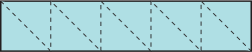
(a)

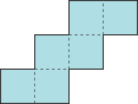
(b)

Figure 1: Two universal hinge patterns in strips. (a) A canonical strip of length $5$. (b) A zig-zag strip of length $6$. The dashed lines are hinges.

The improved surface efficiency and reduced layering of these strip results seem more practical for programmable matter. In addition, the panels of either strip (the facets delineated by hinges) are connected acyclically into a path, making them potentially easier to control. One potential drawback is that the reduced connectivity makes for a flimsier device; this issue can be mitigated by adding tabs to the edges of the strips to make full two-dimensional contacts across seams and thereby increase strength.

We also show in Section 5 an important practical result for our strip foldings: assuming a small lower bound on feature size, we give an algorithm for actually folding the strip into the desired shape, while keeping the panels rigid (flat) and avoiding self-intersection throughout the motion. Such a rigid folding process is important given current fabrication materials, which put flexibility only in the creases between panels [HAB⁺10]. An important limitation, however, is that we assume zero thickness of the material, which would need to be avoided before this method becomes practical.

Our approach is also related to the 1D chain robots of [CDBG11], but based on thin material instead of thick solid chains. Most notably, working with thin material enables us to use a few overlapping layers to make any desired surface without scaling, and still with high efficiency. Essentially, folding long thin strips of sheet material is like a fusion between 1D chains of [CDBG11] and the square sheet folding of [BDDO10, HAB⁺10, ABDR11].

Milling tours.

At the core of our efficient strip foldings are efficient approximation algorithms for milling a grid polyhedron. Motivated by rapid-fabrication CNC milling/cutting tools, milling problems are typically stated in terms of a 2D region called a “pocket” and a cutting tool called a “cutter”, with the goal being to find a path or tour for the cutter that covers the entire pocket. In our situation, the “pocket” is the surface of the grid polyhedron, and the “cutter” is a unit square constrained to move from one grid square of the surface to an (intrinsically) adjacent grid square.

The typical goals in milling problems are to minimize the length of the tour [AFM00] or to minimize the number of turns in the tour [ABD⁺05]. Both versions are known to be strongly NP-hard, even when the pocket is an integral orthogonal polygon and the cutter is a unit square. We conjecture that the minimum-turn problem remains strongly NP-hard when the pocket is a grid polyhedron, but the minimum-length problem turns out to be polynomial: the dual graph is planar and 4-connected and thus Hamiltonian [BL06], so there is an ideal tour visiting each square exactly once, which can be found in linear time [CN89]. (This result also implies a 2-approximation for the metric of length plus turns.)

In our situation, both length and number of turns are important, as both influence the required length of a strip to cover the surface. Thus we develop one algorithm that simultaneously approximates both measures. Such results have also been achieved for 2D pockets [ABD⁺05]; our results are the first we know for surfaces in 3D. Specifically, we develop in Section 3 an approximation algorithm for computing a milling tour of a given grid polyhedron, achieving both a $2$-approximation in length and an $8/3$-approximation in number of turns.

Fonts.

To illustrate the power of strip folding, we designed a typeface, representing each letter of the alphabet by a folding of a $1\times x$ strip for some $x$, as shown in Figure 2. The individual-letters typeface consists of two fonts: the unfolded font is a puzzle to figure out each letter, while the folded font is easy to read. These crease patterns adhere to an integer grid with orthogonal and/or diagonal creases, but are not necessarily subpatterns of the canonical hinge pattern. This extra flexibility gives us control to produce folded half-squares as desired, increasing the font’s fidelity.

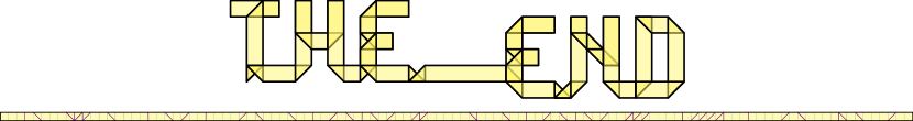
Figure 18: An example of joining together a few letters from our typeface in Figure 2. Unfolding (bottom) not to scale with folding (top).

We have developed a web app that visualizes the font, and chains letters together into one long strip folding. Figure 3, and Figure 18 at the end of the paper, show some examples.

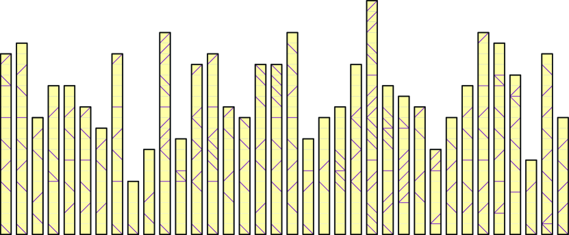
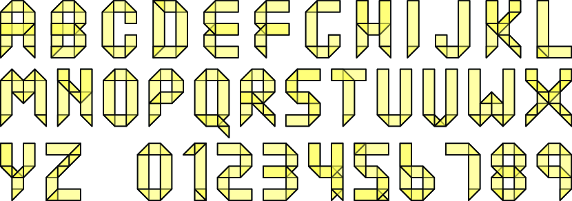
Figure 2: Strip folding of individual letters typeface, A–Z and 0–9: unfolded font (top) and folded font (bottom), where the face incident to the bottom edge remains face-up.

Figure 3: The paper title rendered with our web app, http://erikdemaine.org/fonts/strip/.

2 Universality

In this section, we prove that both the canonical strip and zig-zag strip of Figure 1, of sufficient length, can fold into any grid surface. We begin with milling tours which provide an abstract plan for routing the strip, and then turn to the details of how to manipulate each type of strip.

Dual graph.

Recall that a grid surface consists of one or more grid squares—that is, squares of the 3D cube grid—glued edge-to-edge to form a connected surface (ignoring vertex connections). Define the dual graph to have a dual vertex for each such grid square, and a dual edge between the two dual vertices corresponding to any two grid squares sharing an edge. Our assumption of the grid surface being connected is equivalent to the dual graph being connected.

Milling tours.

A milling tour is a (not necessarily simple) spanning cycle in the dual graph, that is, a cycle that visits every dual vertex at least once (but possibly more than once). Equivalently, we can think of a milling tour as the path traced by the center of a moving square that must cover the entire surface while remaining on the surface, and return to its starting point. Milling tours always exist: for example, we can double a spanning tree of the dual graph to obtain a milling tour of length less than double the given surface area.

At each grid square, we can characterize a milling tour as going straight, turning, or U-turning—intrinsically on the surface—according to which two sides of the grid square the tour enters and exits. If the sides are opposite, the tour is straight; if the sides are incident, the tour turns; and if the sides are the same, the tour U-turns. Intuitively, we can imagine unfolding the surface and developing the tour into the plane, and measuring the resulting planar turn angle at the center of the grid square.

Strip folding.

To prove universality, it suffices to show that a canonical strip or zig-zag strip can follow any milling tour and thus make any grid polyhedron. In particular, it suffices to show how the strip can go straight, turn left, turn right, and U-turn. Then, in 3D, the strip would be further folded at each traversed edge of the grid surface, to stay on the surface. Indeed, U-turns can be viewed as folding onto the opposite side of the same surface, and thus are intrinsically equivalent to going straight; hence we can focus on going straight and making left/right turns.

Canonical strip.

Figure 4 shows how a canonical strip can turn left or right; it goes straight without any folding. Each turn adds $1$ to the length of the strip, and adds $2$ layers to part of the grid square where the turn is made. Therefore a milling tour of length $L$ with $t$ turns of a grid surface can be followed by a canonical strip of length $L+t$. Furthermore, if the milling tour visits each grid square at most $c$ times, then the strip folding has at most $3c$ layers covering any point of the surface.

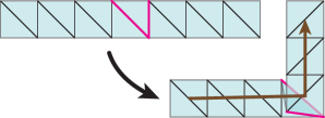
(a)

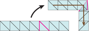
(b)

Figure 4: (a) Left and (b) right turn with a canonical strip.

Zig-zag strip.

Figure 5 shows how to fold a zig-zag strip in order to go straight. In this straight portion, each square of the surface is covered by two squares of the strip. Figure 6 shows left and right turns. Observe that turns require either one or three squares of the strip. Therefore a milling tour of length $L$ with $t$ turns can be followed by a zig-zag strip of length at most $2L+t$. Furthermore, if the milling tour visits each grid square at most $c$ times, then the strip folding has at most $3c$ layers covering any point of the surface.

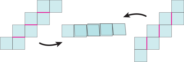
Figure 5: Going straight with a zig-zag strip requires at most two unit squares per grid square. Left and right crease patterns show two possible different parities along the strip.

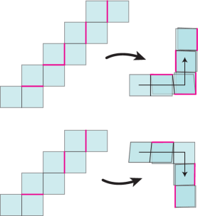
(a)

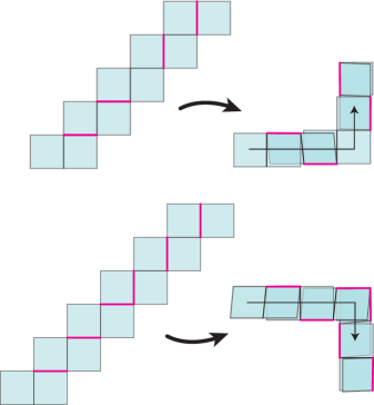
(b)

Figure 6: Turning with a zig-zag strip has two cases because of parity. (a) Turning left at an odd position requires three grid squares, whereas turning right requires one grid square. (b) Turning left at an even position requires one grid square, whereas turning right requires three grid squares.

Proposition 1.

Every grid surface of area $N$ can be folded from a canonical strip of length $4N$, with at most eight layers stacked anywhere, and from a zig-zag strip of length $6N$, with at most twelve layers stacked anywhere.

Proof.

The doubled-spanning-tree milling tour has length $L<2N$, and in the worst case turns at every square visited, i.e., $t<2N$ (counting U-turns at the leaves of the spanning tree). Each square gets visited by the tour at most four times (once per side). The bounds then follow from the analysis above. ∎

The goal in the rest of this paper is to achieve better bounds for grid polyhedra, using more carefully chosen milling tours. For comparison, the best approximation algorithm for milling tours in polygons (not grid surfaces) [AFM00] achieves a bound of $L\leq 1.325\,N$ which, combined with the trivial $t\leq L$ bound, achieves a canonical-strip bound of $t+L\leq 2.65\,N$. We will beat this bound for grid surfaces, reducing to $2N$.

3 Milling Tour Approximation

This section presents a constant-factor approximation algorithm for milling a (genus-0) grid polyhedron $P$ with respect to both length and turns. Specifically, our algorithm is a $2$-approximation in length and an $8/3$-approximation in turns. Our milling tours also have special properties that make them more amenable to strip folding.

Our approach is to reduce the milling problem to vertex cover in a tripartite graph. Then it follows that our algorithm is a $2\alpha$-approximation in turns, where $\alpha$ is the best approximation factor for vertex cover in tripartite graphs. The best known bounds on $\alpha$ are $34/33\leq\alpha\leq 4/3$. Clementi et al. [CCR99] proved that minimum vertex cover in tripartite graphs is not approximable within a factor smaller than $34/33=1.\overline{03}$ unless $\text{P}=\text{NP}$. Theorem 1 of [Hoc83] implies a $4/3$-approximation for minimum weighted vertex cover for tripartite graphs (assuming we are given the 3-partition of the vertex set, which we know in our case). Thus we use $\alpha=4/3$ below. An improved approximation ratio $\alpha$ would improve our approximation ratios, but may also affect the stated running times, which currently assume use of [Hoc83].

3.1 Bands

(a) A grid polyhedron from [CDBG11]	(b) $x$-bands
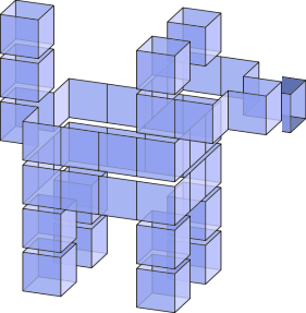
(c) $y$-bands	(d) $z$-bands

Figure 7: Illustration of bands.

The basis for our approximation algorithms is the notion of “bands” for a grid polyhedron $P$; refer to Figure 7. Let $x_{\text{min}}$ and $x_{\text{max}}$ respectively be the minimum and maximum $x$ coordinates of $P$; define $y_{\text{min}},y_{\text{max}},$ $z_{\text{min}},z_{\text{max}}$ analogously. These minima and maxima have integer values because the vertices of $P$ lie on the integer grid. Define the $i$th $x$-slab $S_{x}(i)$ to be the slab bounded by parallel planes $x=x_{\text{min}}+i$ and $x=x_{\text{min}}+i+1$, for each $i\in\{0,1,\dots,x_{\text{max}}-x_{\text{min}}-1\}$. The intersection of $P$ with the $i$th $x$-slab $S_{x}(i)$ (assuming $i$ is in the specified range) is either a single band (i.e., a simple cycle of grid squares in that slab), or a collection of such bands, which we refer to as $x$-bands. Define $y$-bands and $z$-bands analogously.

Two bands overlap if there is a grid square contained in both bands. Each grid square of $P$ is contained in precisely two bands (e.g., if a grid square’s outward normal were in the $+z$-direction, then it would be contained in one $x$-band and one $y$-band). Two bands $B_{1}$ and $B_{2}$ are adjacent if they do not overlap, and a grid square of $B_{1}$ shares an edge with a grid square of $B_{2}$. A band cover for $P$ is a collection of $x$-, $y$-, and $z$-bands that collectively cover the entire surface of $P$. The size of a band cover is the number of its bands.

3.2 Cover Bands

The starting point for the milling approximation algorithm is to find an approximately minimum band cover, as the minimum band cover is a lower bound on the number of turns in any milling tour:

Proposition 2.

[ABD⁺05, Lemma 4.9] The size of a minimum band cover of a grid polyhedron $P$ is a lower bound on the number of turns in any milling tour of $P$.

Proof.

Consider a milling tour of $P$ with $t$ turns. Extend the edges of the tour of $P$ into bands. This yields a band cover of size at most $t$. ∎

Next we describe how to find a near-optimal band cover. Consider the graph $G_{P}$ with one vertex per band of a grid polyhedron $P$, connecting two vertices by an edge if their corresponding bands overlap. It turns out that an (approximately minimum) vertex cover in $G_{P}$ will give us an (approximately minimum) band cover in $P$:

Proposition 3.

A vertex cover for $G_{P}$ induces a band cover of the same size and vice versa.

Proof.

Because the vertices of $G_{P}$ correspond to bands, it suffices to show that a set of bands $S$ covers all the grid squares of $P$ if and only if the corresponding vertex set $V_{S}$ covers all the edges of $G_{P}$. First suppose that $V_{S}$ covers the edges of $G_{P}$. Observe that a grid square is contained in two bands and those bands overlap, so there is a corresponding edge in $G_{P}$. Because $V_{S}$ covers the edge in $G_{P}$, $S$ must cover the grid square.

Conversely, suppose $S$ covers all the grid squares of $P$. Any edge of $G_{P}$ corresponds to two overlapping bands, which overlap in a grid square (in fact, they overlap in at least two grid squares because $P$ has genus $0$). Because the grid square is in exactly two bands, and $S$ covers the grid square, then $V_{S}$ covers the corresponding edge in $G_{P}$. ∎

Because the bands fall into three classes ($x$-, $y$-, and $z$-), with no overlapping bands within a single class, $G_{P}$ is tripartite. Hence we can use an $\alpha$-approximation algorithm for vertex cover in tripartite graphs to find an $\alpha$-approximate vertex cover in $G_{P}$ and thus an $\alpha$-approximate band cover of $P$.

3.3 Connected Bands

Our next goal will be to efficiently tour the bands in the cover. Given a band cover $S$ for a grid polyhedron $P$, define the band graph $G_{S}$ to be the subgraph of $G_{P}$ induced by the subset of vertices corresponding to $S$. We will construct a tour of the bands $S$ based on a spanning tree of $G_{S}$. Our first step is thus to show that $G_{S}$ is connected (Lemma 5 below). We do so by showing that adjacent bands (as defined in Section 3.1) are in the same connected component of $G_{S}$, using the following lemma of Genc [Gen08]:

Lemma 4.

[Gen08] For any band $B$ in a grid polyhedron $P$, let $N_{B}$ be the bands of $P$ overlapping $B$. (Equivalently, $N_{B}$ is the set of neighbors of $B$ in $G_{P}$). Then the subgraph of $G_{P}$ induced by $N_{B}$ is connected.

Lemma 5.

If $S$ is a band cover for a grid polyhedron $P$, then the graph $G_{S}$ is connected.

Proof.

First define an auxiliary graph $H_{S}$ which has edges between adjacent bands in addition to edges between overlapping bands. Because the surface of $P$ is connected, $H_{S}$ is connected, because there is an (orthogonal) path on the surface of $P$ between any two bands and this path induces a sequence of edges in $H_{S}$. We will argue that $G_{S}$ has the same connectivity as $H_{S}$, and thus is connected.

Now consider any pair of adjacent bands $B_{1}$ and $B_{2}$ in $S$, forming an edge in $H_{S}$ but not $G_{S}$. Refer to Figure 8. Because $B_{1}$ and $B_{2}$ are adjacent, there exists grid squares $g_{1}\in B_{1}$ and $g_{2}\in B_{2}$ which share an edge $e$. Let $B_{3}$ be the band through grid squares $g_{1}$ and $g_{2}$. If $B_{3}$ is in the band cover, then the vertices corresponding to $B_{1}$ and $B_{2}$ are in the same connected component of $G_{S}$ because $B_{3}$ overlaps both $B_{1}$ and $B_{2}$. Thus suppose that $B_{3}$ is not in $S$. Then each of the bands overlapping $B_{3}$ (excluding $B_{3}$ itself) must be in $S$; otherwise there would be an uncovered grid square of $B_{3}$. Let $N_{3}$ denote this set of bands. By Lemma 4, the subgraph $G_{P}[N_{3}]$ of $G_{P}$ induced by $N_{3}$ is connected. Now because $G_{P}[N_{3}]$ is also a subgraph of $G_{S}$, we have that the vertices corresponding to $B_{1}$ and $B_{2}$ are in the same connected component of $G_{S}$. ∎

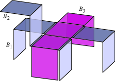
Figure 8: Bands $B_{1}$, $B_{2}$, and $B_{3}$ in the proof of Lemma 5.

3.4 Band Tour

Now we can present our algorithm for transforming a band cover into an efficient milling tour.

Theorem 6.

Let $P$ be a grid polyhedron with $N$ grid squares. In $O(N^{2}\log N)$ time, we can find a milling tour of $P$ that is a $2$-approximation in length and an $8/3$-approximation (or more generally, a $2\alpha$-approximation) in turns.

Proof.

We start with an $\alpha$-approximation to the minimum vertex cover of $G_{P}$, such as the $\alpha=4/3$ algorithm of [Hoc83]. Then we convert this vertex cover into a band cover $S$. By Proposition 3, $S$ is an $\alpha$-approximation for the minimum band cover for $P$. Construct the band graph $G_{S}$, and construct a spanning tree $T$ of $G_{S}$, which exists as $G_{S}$ is connected by Lemma 5. We now describe how to obtain a milling tour by touring $T$. (Note that we will use “nodes of the tree” and “bands of $S$” interchangeably.)

Consider the band $r$ which is the root of $T$. Pick an arbitrary starting grid square $p_{r}$ on $r$, as well as a starting direction along band $r$. Now order the children of $r$ based on the order in which they are first encountered as we walk along $r$ starting at $p_{r}$. We will visit the children of $r$ in this order when we follow the tour. Let the ordered children of $r$ be denoted by $u_{1},\dots,u_{k}$. Walking along $r$, when we hit a child $u_{i}$ (say at grid square $p_{i}$) which has not yet been visited, we turn right (or left, it doesn’t matter) onto band $u_{i}$ and recursively visit the children of $u_{i}$ as we are walking, until we eventually return back to $r$ which requires an additional turn (in the opposite direction of the turn onto $u_{i}$) to get back onto $r$ and resume walking along $r$. Because turns only ever occur between parent and child pairs, we can bound the number of turns in terms of the number of edges of $T$. In particular, there are two turns per edge of $T$, one turn from the parent band onto the child band, and one turn from the child band back onto the parent band. Thus the total number of turns is

$$2\,|E(T)|=2\cdot(|S|-1)\leq 2\,\alpha\cdot\text{OPT}_{BC},$$

where $\text{OPT}_{BC}$ is the size of the minimum band cover for $P$. Now by Proposition 2, $\text{OPT}_{BC}$ is a lower bound on the number of turns necessary, so this yields a $2\alpha$-approximation in turns.

Next we argue that each grid square is visited at most twice, implying a $2$-approximation in length. Each grid square is contained in exactly two bands of $P$, at least one of which must be in $S$ because $S$ is a band cover. Let $g$ be a grid square of $P$. If $g$ is contained in just one band of $S$, then it is visited only once, namely when that band is traversed by the milling tour. Thus suppose $g$ is contained in two bands, $S_{1}$ and $S_{2}$, of $S$. There are two cases to consider. In the first case, neither band is a parent of the other band. So $g$ will be visited exactly two times, once when $S_{1}$ is traversed, and a second time when $S_{2}$ is traversed. (We call such a $g$ a straight junction due to the way in which it is traversed, as Figure 9(a) depicts.) The second case to consider is when one of the bands is a parent of the other band. Without loss of generality, assume $S_{1}$ is a parent of $S_{2}$. Then $g$ will be visited twice, once when turning from $S_{1}$ onto $S_{2}$, and a second time when turning from $S_{2}$ back onto $S_{1}$. (We call $g$ a turn junction in this case, as Figure 9(b) depicts. Notice that the turn from $S_{1}$ onto $S_{2}$ is in the opposite direction of the turn from $S_{2}$ onto $S_{1}$. This fact will be useful when we explore applications of this algorithm to strip folding, although it is not immediately of use.) Hence each grid square is visited at most twice.

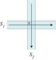
(a)

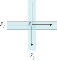
(b)

Figure 9: (a) A straight junction, and (b) a turn junction.

Finally we analyze the running time of this algorithm. The time to compute an $\alpha$-approximation for the minimum band cover of $P$ is the same as the time to compute an $\alpha$-approximation for the minimum vertex cover for $G_{P}$. Because each grid square corresponds to an edge of $G_{P}$ and each edge of $G_{P}$ corresponds to two unique grid squares, the number of edges $|E(G_{P})|=N/2$. The number of vertices $|V(G_{P})|$ is the number of unit bands of $P$, which is at most $N$. By Theorem 1 of [Hoc83], the time to compute a $4/3$-approximation for the minimum vertex cover for $G_{P}$ is $O(|V(G_{P})||E(G_{P})|\log\,|V(G_{P})|)$, which is thus $O(N^{2}\log\,N)$. This term is dominant in the running time for computing the milling tour, establishing the theorem. ∎

We now state some additional properties of any milling tour produced by the approximation algorithm of Theorem 6, which will be useful for later applications to strip folding in Section 4.

Proposition 7.

Let $P$ be a grid polyhedron, and consider a milling tour of $P$ obtained from the approximation algorithm of Theorem 6. Then the following properties hold:

1. A grid square of $P$ is either visited once, in which case it is visited by a straight part of the tour; or it is visited twice, in one of the two configurations of Figure 9 (a straight junction or a turn junction—in particular, never a U-turn).

2. In the case of a turn junction, the length of the milling tour between the two visits to the grid square (counting only one of the two visits to the grid square in the length measurement) is even.

3. The tour can be modified to alternate between left and right turns (without changing its length or the number of turns).

Proof.

Property (1) has already been established in the proof of Theorem 6 (see the paragraph on the length calculation which bounds the number of times each grid square is visited and how a grid square can be visited).

The proof of Property (2) follows by induction on the number of bands in the spanning tree from which the milling tour was constructed. The base case of one band is trivial as a band has an even number of grid squares. Thus suppose Property (2) holds for all such trees with fewer than $k$ bands for some $k>1$. Assume we have a tree $T$ with $k$ bands. Consider a leaf of $T$. Let $B_{2}$ be the band corresponding to the leaf, and let $B_{1}$ be the band corresponding to the parent of $B_{2}$. If we remove $B_{2}$ from $T$ we get a tree $T^{\prime}$ with $k-1$ bands, so by induction Property (2) holds. Adding $B_{2}$ back, the length of the milling tour between the two visits to a grid square will either be unaffected (in the case where the subtree rooted at the child band corresponding to the grid square does not contain $B_{2}$) or it will increase by $|B_{2}|$ (i.e., the number of grid squares in $B_{2}$) which is even. Thus Property (2) still holds.

Property (3) follows by the way we constructed the milling tour as a tour of a spanning tree of bands. We had the freedom to choose whether to turn left or right from a parent band onto a child band, and then the turn direction from the child back onto the parent was forced to be the opposite turn direction. Hence we can choose the turn directions from parent bands onto child bands in such a way that maintains alternation between left and right turns. ∎

3.5 Polynomial Time

The algorithm described above is polynomial in the surface area $N$ of the grid polyhedron, or equivalently, polynomial in the number of unit cubes making up the polyomino solid. For our application to strip folding, this is polynomial in the length of the strip, and thus sufficient for most purposes. On the other hand, polyhedra are often encoded as a collection of $n$ vertices and faces, with faces possibly much larger than a unit square. In this case, the algorithm runs in pseudopolynomial time.

Although we do not detail the approach here, our algorithm can be modified to run in polynomial time. To achieve this result, we can no longer afford to deal with unit bands directly, because their number is polynomially related to the number $N$ of grid squares, not the number $n$ of vertices. To achieve polynomial time in $n$, we concisely encode the output milling tour using “fat” bands rather than unit bands, which can then be easily decoded into a tour of unit bands. By making each band as wide as possible, their number is polynomially related to $n$ instead of $N$. Details of an $O(n^{3}\log n)$-time milling approximation algorithm (with the same approximation bounds as above) can be found in [Ben11].

4 Strip Foldings of Grid Polyhedra

In this section, we show how we can use the milling tours from Section 3 to fold a canonical strip or zig-zag strip efficiently into a given (genus-0) grid polyhedron. For both strip types, define the length of a strip to be the number of grid squares it contains; refer to Figure 1. For a strip folding of a polyhedron $P$, define the number of layers covering a point $q$ on $P$ to be the number of interior points of the strip that map to $q$ in the folding, excluding crease points, that is, points lying on a hinge that gets folded by a nonzero angle. (This definition may undercount the number of layers along one-dimensional creases, but counts correctly at the remaining two-dimensional subset of $P$.) We will give bounds on the length of the strip and also on the maximum number of layers of the strip covering any point of the polyhedron.

4.1 Canonical Strips

The main idea for canonical strips is that Properties (1) and (3) of Proposition 7 allow us to make turns as shown in Figure 10, so that we do not waste an extra square of the strip per turn.

Theorem 8.

If a grid polyhedron $P$ has a milling tour $\mathcal{T}$ of length $L$ with $t$ turns, and $\mathcal{T}$ satisfies Properties (1) and (3) of Proposition 7, then $P$ can be covered by a folding of a canonical strip of length $L$ with at most two layers covering any point of $P$. Furthermore, the number of hinges folded by $180^{\circ}$ is $t$.

Proof.

Because $\mathcal{T}$ alternates between left and right turns (Property (3)), the canonical strip can follow $\mathcal{T}$ by making a single diagonal fold by $180^{\circ}$ at each turn (instead of the more complicated folds given by Figure 4). (It is the fact that the canonical strip has all the diagonal hinges in the same direction that forces alternation between left and right turns from folding only at diagonal hinges.) Furthermore, by Property (1), if $\mathcal{T}$ turns at a grid square, then the grid square is visited twice and must correspond to a turn junction as shown in Figure 9(b). Thus we can cover turn junctions with the canonical strip as shown in Figure 10. Notice that one grid square of the strip is used per turn, and there are only two layers of the strip covering a turn junction.

By Property (1), if $\mathcal{T}$ goes straight at a grid square, then it is visited at most twice by $\mathcal{T}$ (and in the case of being visited twice, it is a straight junction as shown in Figure 9(a)). Going straight along $\mathcal{T}$ uses just one grid square of the strip, so a straight junction is covered by two layers of the strip. The total length of the strip used is thus $L$, and there are at most two layers of the strip covering each point of $P$. The number of hinges folded by $180^{\circ}$ is exactly one turn in the milling tour, which is $t$; all folds made for the strip to follow the surface are by $90^{\circ}$ because, by Property (1), the tour has no U-turns. ∎

Corollary 9.

Let $P$ be a grid polyhedron, and let $N$ be the number of grid squares of $P$. Then $P$ can be covered by a folding of a canonical strip of length $2N$, and with at most two layers covering any point of $P$.

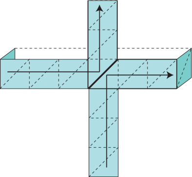
Figure 10: A turn junction for a canonical strip. The parent band is vertical and the child band is horizontal. The canonical strip starts out traveling upwards, turns right onto the child, visits the child and its subtree, and returns from the child by turning left back onto the parent band. Notice that each turn uses just one grid square of the canonical strip, and there are only two layers of paper covering the turn junction grid square.

4.2 Zig-Zag Strips

For zig-zag strips, we instead use Properties (1) and (2) of Proposition 7:

Theorem 10.

If a grid polyhedron $P$ has a milling tour $\mathcal{T}$ of length $L$ with $t$ turns, and $\mathcal{T}$ satisfies properties (1) and (2) of Proposition 7, then $P$ can be covered by a folding of a zig-zag strip of length $2L$ with at most four layers covering any point of $P$. Furthermore, the number of hinges folded by $180^{\circ}$ is $L$.

Proof.

By Property (1), $\mathcal{T}$ has no U-turns. If we follow the tour with a zig-zag strip using the turn gadgets in Figure 6, then, at even positions, left turns require one unit square of the strip and right turns require three unit squares, while at odd positions, left turns require three unit squares and right turns require one unit square. Hence the positions along $\mathcal{T}$ alternate between left turns being “easy” or being “hard” for the zig-zag strip, and similarly for right turns.

Consider a grid square $g$ corresponding to a turn junction of $\mathcal{T}$. Then $g$ is visited twice by the tour, with the first visit and second visit having opposite turn directions (i.e., if the first visit is a left turn, the second visit will be a right turn, and vice versa). Now by Property (2), the length of the milling tour between the first and second visit to $g$ (counting $g$ itself only once) is even, and so the second visit to $g$ has the same parity as the first visit to $g$. Now because the turns are in opposite directions, one of the turns costs one grid square of the zig-zag strip, while the other turn costs three grid squares of the zig-zag strip as explained above. Hence turn junctions are covered by four grid squares of the zig-zag strip.

By Property (1), the only other types of grid squares to consider are a straight junction, or a grid square which is visited exactly once by going straight. Figure 5 illustrates that going straight at a grid square requires at most two squares of the zig-zag strip. And because a straight junction is visited twice, at most four squares of the zig-zag strip cover a straight junction. Combining this with the turn junction coverage of four, we have at most four layers of the strip covering any point of $P$.

Now we are ready to measure the total length of the zig-zag strip used. The length of $\mathcal{T}$ spent going straight is $L-t$; thus we use $\leq 2(L-t)$ grid squares of the strip for going straight. The length of $\mathcal{T}$ spent on turns is $t$, and half of the turns cost $1$ grid square while the other half cost $3$ grid squares, so we spend $\leq t/2+3t/2=2t$ grid squares of the strip for turns. Thus the total number of grid squares of the strip used is at most $2(L-t)+2t=2L$.

Finally we bound the number of $180^{\circ}$ folds of the strip. At portions of the tour going straight, we use one $180^{\circ}$ fold per unit of length, and thus $L-t$ such folds are dedicated to going straight. For turns, half of the turns require two $180^{\circ}$ folds, whereas the other half require no $180^{\circ}$ folds. Hence we obtain a total of $L-t+2(t/2)=L$ $180^{\circ}$ folds. ∎

Corollary 11.

Let $P$ be a grid polyhedron, and let $N$ be the number of grid squares of $P$. Then $P$ can be covered by a folding of a zig-zag strip of length $4N$, and with at most four layers covering any point of $P$.

By coloring the two sides of the zig-zag strip differently, we can also bicolor the surface of $P$ in any pattern we wish, as long as each grid square is assigned a uniform color. We do not prove this result formally here, but mention that the bounds in length would become somewhat worse, and the rigid motions presented in Section 5 do not work in this setting.

5 Rigid Motion Avoiding Collision

So far we have focused on just specifying a final folded state for the strip, and ignored the issue of how to continuously move the strip into that folded state. In this section, we show how to achieve this using a rigid folding motion, that is, a continuous motion that keeps all polygonal faces between hinges rigid/planar, bending only at the hinges, and avoids collisions throughout the motion. Rigid folding motions are important for applications to real-world programmable matter made out of stiff material except at the hinges. Our approach may still suffer from practical issues, as it requires a large (temporary) accumulation of many layers in an accordion form.

We prove that, if the grid polyhedron $P$ has feature size at least $2$, then we can construct a rigid motion of the strip folding without collision. (By feature size at least $2$, we mean that every exterior voxel of $P$ is contained in some $2\times 2\times 2$ box with empty interior. For example, Figure 7(a) does not have this property because of the voxels between adjacent legs and ears.) If the grid polyhedron we wish to fold does not have this property, then one solution is to scale the polyhedron by a factor of $2$, and then the results here apply.

5.1 Approach

(a)

(b)

Figure 11: For both strip types, we can fold the unused portion of the strip (initially, all of it) into an accordion to avoid collision during the folding motion. (a) Canonical strip. (b) Zig-zag strip, with hinges drawn thick for increased visibility.

Our approach is to keep the yet-unused portion of the strip folded up into an accordion and then to unfold only what is needed for the current move: straight, left, or right. Figure 11 shows the accordion state for the canonical strip and for the zig-zag strip. We will perform the strip folding in such a way that the strip never penetrates the interior of the polyhedron $P$, and it never weaves under previous portions of the strip. Thus, we could wrap the strip around $P$’s surface even if $P$’s interior were already a filled solid. This restriction helps us think about folding the strip locally, because some of $P$’s surface may have already been folded (and it thus should not be penetrated) by earlier parts of the strip.

It suffices to show, regardless of the local geometry of the polyhedron at the grid square where the milling tour either goes straight or turns, and regardless of whether the accordion faces up or down relative to the grid square it is covering (see Figure 12), that we can maneuver the accordion in a way that allows us to unroll as many squares as necessary to perform the milling-tour move. A naïve enumeration of the combinations of local geometry, accordion facing up or down, tour move (left turn, right turn, or straight), and the type of strip being folded, would lead to a large number of cases, but fortunately we can narrow this space down to a small number of essential cases.

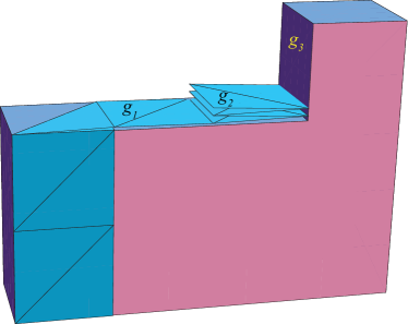
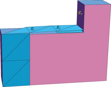
Figure 12: The accordion covering grid square $g_{2}$ (a) face up, and (b) face down.

We use the following notation to describe such a local case. Let $g_{1}$, $g_{2}$, and $g_{3}$ denote the grid square previously visited by the strip, the current grid square, and the next grid square the strip will visit, respectively. Let $e_{12}$ refer to the edge shared by $g_{1}$ and $g_{2}$, and let $e_{23}$ refer to the edge shared by $g_{2}$ and $g_{3}$. The local geometry of $P$ at $g_{2}$ is determined entirely by the position of $e_{12}$ relative to $e_{23}$ (if they are adjacent edges of $g_{2}$, then we have a turn, and if they opposite edges, then we have a straight) and whether each of those edges is reflex ($270^{\circ}$ dihedral angle), flat ($180^{\circ}$ dihedral angle), or convex ($90^{\circ}$ dihedral angle), respectively.

Next we reduce the number of cases we need to consider. First, left and right turns are symmetric, so we consider only right turns. Second, when the accordion is facing up, going straight or turning is relatively straightforward. Figure 13 shows the moves for a canonical strip going straight (an extrinsic rotation of some multiple of $90^{\circ}$), and one case of turning (when $e_{23}$ is flat or convex); we omit the remaining turning case (when $e_{23}$ is reflex) as it is similar to the F–R turn case below. The same strategy for going straight can be applied to the zig-zag strip, unfolding the appropriate crease to go left, straight, or right. Thus we focus our case analysis on cases where the accordion is facing down. Maneuvering the strip is more difficult in this case, because the accordion naturally wants to unfold into the interior of $P$, which we forbid (and which could be a real problem because the surface of $P$ may have already been covered by previous portions of the strip).

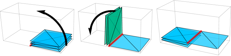
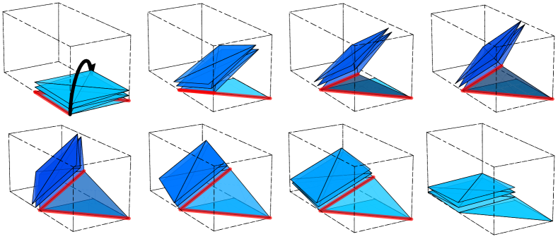
Figure 13: Continuous folding motion within a $1\times 1\times 2$ box for canonical strip, face-up cases. (a) Straight. (b) Turn where $e_{23}$ is flat.

5.2 Canonical Strip

For the canonical strip, there are two turn cases and one straight case.

Turns.

In the F–R turn case, $e_{12}$ is a flat edge and $e_{23}$ is a reflex edge, as illustrated in Figure 14(a). The moves we present for this case also work for any combination of $e_{12}$ being convex or flat and $e_{23}$ being reflex, flat, or convex. Hence these moves cover all turn cases except for the R–R case where $e_{12}$ and $e_{23}$ are both reflex; see Figure 15(a).

Figures 14(b) and 15(b) illustrate the moves for the F–R and R–R turn cases, respectively. The F–R turn case does not exploit feature size, which is why the moves here still work for any combination of $e_{12}$ being convex or flat and $e_{23}$ being reflex, flat, or convex. The R–R turn case uses that the dashed voxel in Figure 15 one unit away from $g_{1}$ must be empty because we assumed feature size at least $2$, and so the moves here rely on the specific position of $g_{1}$ relative to $g_{2}$ (i.e., they rely on $e_{12}$ being a reflex edge).

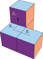
(a)

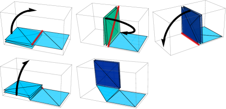
(b)

Figure 14: Continuous folding motion for canonical strip, F–R turn case. (a) Local geometry. (b) Moves within a $1\times 1\times 2$ box for a face-down canonical accordion.

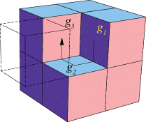
(a)

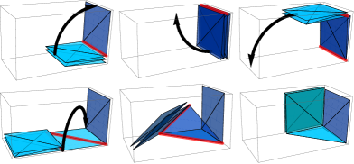
(b)

Figure 15: Continuous folding motion for canonical strip, R–R turn case. (a) Local geometry. The dashed voxel beginning one unit away from $g_{1}$ must be empty because we assumed feature size at least $2$. (b) Moves within a $1\times 1\times 2$ box for a face-down canonical accordion.

Straight.

In the R–C straight case, $e_{12}$ is a reflex edge and $e_{23}$ is a convex edge; see Figure 16(a). Figure 16(b) shows the moves for this straight case where the canonical accordion lies face-down on $g_{2}$. The moves for this case can be modified for any straight case (i.e., any combination of edge types for $e_{12}$ and $e_{23}$) except the R–R case when both $e_{12}$ and $e_{23}$ are reflex, but this case is impossible while having the exterior voxel adjacent to $g_{2}$ in an empty $2\times 2\times 2$ box.

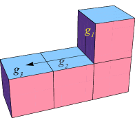
(a)

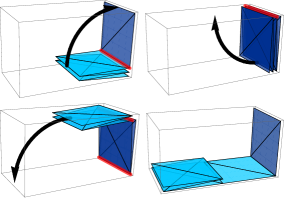
(b)

Figure 16: Continuous folding motion for canonical strip, R–C straight case. (a) Local geometry. (b) Moves within a $1\times 1\times 2$ box for a face-down canonical accordion.

5.3 Zig-Zag Strip

The analysis for the zig-zag strip accordion moves is slightly more complicated because we now also have to consider whether a turn costs $1$ unit or $3$ units, as the moves can be different depending upon which turn-cost case we are in.

Turns.

There are four turn cases for the zig-zag gadget that need to be considered:

F–R–$1$:

$e_{12}$ is flat, $e_{23}$ is reflex, and the turn costs $1$;

R–F–$*$:

$e_{12}$ is reflex, $e_{23}$ is flat, and the turn costs $1$ or $3$ (the moves work regardless of the turn cost);

R–R–$1$:

$e_{12}$ and $e_{23}$ are reflex, and the turn costs $1$; and

R–R–$3$:

$e_{12}$ and $e_{23}$ are reflex, and the turn costs $3$.

We explain briefly why these are the only turn cases that need to be considered. The moves for case F–R–1 also work when $e_{12}$ is convex and $e_{23}$ is reflex with turn cost $1$. The moves for case R–F–$*$ also work for any combination of edge types for $e_{12}$ and $e_{23}$ where $e_{23}$ is not reflex. The moves for case R–R–3 work when $e_{12}$ is flat or convex and $e_{23}$ is reflex with turn cost $3$. Thus these cases collectively cover all possible cases we need to consider for the zig-zag strip.

For brevity, we show the moves for just one of the turn cases, R–F–$*$. Figure 17 illustrates turn case R–F–$1$. The same moves also work for turn cost $3$.

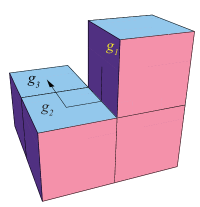
(a)

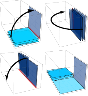
(b)

Figure 17: Continuous folding motion for zig-zag strip, R–F–$1$ turn case. (a) Local geometry. (b) Moves within a $1\times 1\times 2$ box for a face-down zig-zag accordion where the turn costs $1$. These moves also work for turn cost $3$, and for any combination of edge types for $e_{12}$ and $e_{23}$ not having $e_{23}$ reflex.

Straight.

As with the canonical strip, it suffices to consider the R–C straight case where $e_{12}$ is a reflex edge and $e_{23}$ is a convex edge. The moves for this case with the zig-zag strip are analogous to those in Figure 16 presented for the canonical strip, so we do not repeat them.

References

- [ABD+05] Esther M. Arkin, Michael A. Bender, Erik D. Demaine, Sándor P. Fekete, Joseph S. B. Mitchell, and Saurabh Sethia. Optimal covering tours with turn costs. SIAM Journal on Computing, 35(3):531–566, 2005.
- [ABDR11] Byoungkwon An, Nadia Benbernou, Erik D. Demaine, and Daniela Rus. Planning to fold multiple objects from a single self-folding sheet. Robotica, 29(1):87–102, 2011. Special issue on Robotic Self-X Systems.
- [AFM00] Esther M. Arkin, Sándor P. Fekete, and Joseph S. B. Mitchell. Approximation algorithms for lawn mowing and milling. Computational Geometry: Theory and Applications, 17(1–2):25–50, 2000.
- [BDDO10] Nadia M. Benbernou, Erik D. Demaine, Martin L. Demaine, and Aviv Ovadya. Universal hinge patterns to fold orthogonal shapes. In Origami5: Proceedings of the 5th International Conference on Origami in Science, Mathematics and Education, pages 405–420. A K Peters, Singapore, 2010.
- [Ben11] Nadia M. Benbernou. Geometric Algorithms for Reconfigurable Structures. PhD thesis, Massachusetts Institute of Technology, September 2011.
- [BL06] Olivier Bodini and Sandrine Lefranc. How to tile by dominoes the boundary of a polycube. In Attila Kuba, László G. Nyúl, and Kálmán Palágyi, editors, Proceedings of the 13th International Conference on Discrete Geometry for Computer Imagery, pages 630–638, Szeged, Hungary, October 2006.
- [CCR99] Andrea E. F. Clementi, Pierluigi Crescenzi, and Gianluca Rossi. On the complexity of approximating colored-graph problems. In Proceedings of the 5th Annual International Conference on Computing and Combinatorics, volume 1627 of Lecture Notes in Computer Science, pages 281–290, 1999.
- [CDBG11] Kenneth C. Cheung, Erik D. Demaine, Jonathan Bachrach, and Saul Griffith. Programmable assembly with universally foldable strings (moteins). IEEE Transactions on Robotics, 27(4):718–729, 2011.
- [CN89] Norishige Chiba and Takao Nishizeki. The Hamiltonian cycle problem is linear-time solvable for 4-connected planar graphs. Journal of Algorithms, 10(2):187–211, 1989.
- [DDM00] Erik D. Demaine, Martin L. Demaine, and Joseph S. B. Mitchell. Folding flat silhouettes and wrapping polyhedral packages: New results in computational origami. Computational Geometry: Theory and Applications, 16(1):3–21, 2000.
- [DT17] Erik D. Demaine and Tomohiro Tachi. Origamizer: A practical algorithm for folding any polyhedron. In Proceedings of the 33rd International Symposium on Computational Geometry, pages 34:1–34:15, Brisbane, Australia, July 2017.
- [Gen08] Burkay Genc. Reconstruction of Orthogonal Polyhedra. PhD thesis, University of Waterloo, 2008.
- [HAB+10] E. Hawkes, B. An, N. M. Benbernou, H. Tanaka, S. Kim, E. D. Demaine, D. Rus, and R. J. Wood. Programmable matter by folding. Proceedings of the National Academy of Sciences of the United States of America, 107(28):12441–12445, 2010.
- [Hoc83] Dorit S. Hochbaum. Efficient bounds for the stable set, vertex cover and set packing problems. Discrete Applied Mathematics, 6(3):243–254, 1983.
- [Lan96] Robert J. Lang. A computational algorithm for origami design. In Proceedings of the 12th Annual ACM Symposium on Computational Geometry, pages 98–105, Philadelphia, PA, May 1996.
- [LD06] Robert J. Lang and Erik D. Demaine. Facet ordering and crease assignment in uniaxial bases. In Origami4: Proceedings of the 4th International Conference on Origami in Science, Mathematics, and Education, pages 189–205, Pasadena, California, September 2006. A K Peters.