Typical length scales in conducting disorderless networks

Abstract

We take advantage of a recently established equivalence, between the intermittent dynamics of a deterministic nonlinear map and the scattering matrix properties of a disorderless double Cayley tree lattice of connectivity $K$, to obtain general electronic transport expressions and expand our knowledge of the scattering properties at the mobility edge. From this we provide a physical interpretation of the generalized localization length.

I Introduction

Very recently, it has been found that the electronic scattering properties of a layered linear periodic structure and those of a regular nonlinear network model are described exactly by the dynamics of intermittent low-dimensional nonlinear maps MM-R ; Jiang ; Victor2013 . The presence of these maps is a consequence of the combination rule of scattering matrices when the scattering systems are built via consecutive replication of an element or motif. This new insight implies an equivalence between wave transport phenomena in classical wave systems, or electronic transport through quantum systems, and the dynamical properties of low-dimensional nonlinear maps, specially at the onset of chaos. This is a remarkable property in that a system with many degrees of freedom experiences a radical reduction of these, so that its description is completely provided by only a few variables.

In particular, the band structure associated with scatterers arranged as a regular double Cayley tree (see Fig.1) corresponds to dynamical properties of attractors of dissipative low-dimensional nonlinear maps MM-R . The properties of the dimensionless conductance in the crystalline limit reflect the periodic or chaotic nature of the attractors. The transition between the insulating to conducting phases can be seen as the transition along one of the known routes to (or out of) chaos, the tangent bifurcation that exhibits intermittent dynamics in its vicinity Schuster . While the conductance displays an exponential decay with size in the evolution towards the crystalline limit, it obeys instead a $q$-exponential form at the transition. A similar behavior can be found for a locally periodic structure where the wave function also decays exponentially in a regular band (or regular attractor) and a $q$-exponential decay with system size at the mobility edge (or onset of chaos) Victor2013 . In the latter model, the typical decay length is related to the mean free path. It is expected that the same occurs for the former model.

In the present paper we generalize our treatment for the scattering properties across a double Cayley tree of arbitrary connectivity $K$. We focus on the conductance. Our purpose is to find the most general expressions for the band edges at the borderline behavior of the conductance toward the crystalline limit. We also determine a general expression for the length scale at the transition. In the next section we establish the recurrence relation for the scattering matrices of double Cayley trees of consecutive sizes. Next, we diagonalize this relation in order to reduce the matrix expression to two equivalent nonlinear maps for their eigenphases. This allows us to analize the system size dependence of the sensitivity to initial conditions for the different types of attractors of the map, including that at the transition. In Section III we consider the implications for electronic transport. We conclude in Section IV.

II Scattering and deterministic maps

II.1 Recurrence relation for the scattering matrix of a double Cayley tree

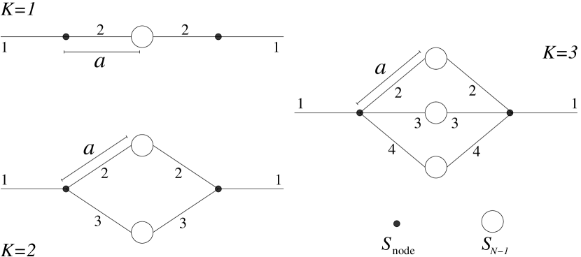
Figure 1: Scheme of double Cayley trees of connectivity $K=1$, $K=2$ and $K=3$ at generation $N$. The leads indexed by 1 are coupled by the nodes, each described by the scattering matrix $S_{\rm{node}}$. $S_{N-1}$ is the scattering matrix at generation $N-1$.

We consider an ordered double Cayley tree of connectivity $K\geq 1$. In Fig. 1 we show the double Cayley trees for $K=1$, $K=2$ and $K=3$. We assume that the leads which connect two adjacent nodes, separated by a lattice constant $a$ (they are indexed by 2, 3, $\ldots K+1$ in the figure), are one-dimensional perfect wires. Also, we assume that each node is described by the same symmetric scattering matrix, which is of dimension $K+1$ and of the form

$$S_{\rm{node}}=\left(\begin{array}[]{c|ccccc}S_{11}&S_{12}&S_{12}&\cdots&S_{12}&S_{12}\\ \hline\cr S_{12}&S_{22}&S_{23}&\cdots&S_{23}&S_{23}\\ S_{12}&S_{23}&S_{22}&\cdots&S_{23}&S_{23}\\ \vdots&\vdots&\vdots&\ddots&\vdots&\vdots\\ S_{12}&S_{23}&S_{23}&\cdots&S_{22}&S_{23}\\ S_{12}&S_{23}&S_{23}&\cdots&S_{23}&S_{22}\\ \end{array}\right).$$ (1)

The matrix $S_{\rm{node}}$ couples symmetrically the incoming lead 1 to the leads 2, 3, $\ldots K+1$, which are assumed to be equivalent. Flux conservation restricts $S_{\rm{node}}$ to be a unitary matrix; this condition is expressed by the three equations

$$|S_{11}|^{2}+K|S_{12}|^{2} = 1,$$ (2)

$$S^{*}_{11}S_{12}+S^{*}_{12}\left[S_{22}+(K-1)S_{23}\right] = 0,$$ (3)

$$|S_{12}|^{2}+|S_{22}|^{2}+(K-1)|S_{23}|^{2} = 1.$$ (4)

Eq. (2) restricts $S_{12}$ to $|S_{12}|\leq 1/\sqrt{K}$. Also, this equation can be written in terms of the reflection and transmission coefficients of the node, $R_{\rm{node}}$ and $T_{\rm{node}}$, respectively, as

$$R_{\rm{node}}+T_{\rm{node}}=1,\quad\mbox{with}\quad R_{\rm{node}}=|S_{11}|^{2}\quad\mbox{and}\quad T_{\rm{node}}=K|S_{12}|^{2}.$$ (5)

A recursion relation for the scattering matrix can be found using the combination rule of scattering matrices. We obtain the $2\times 2$ scattering matrix at a given generation $N$, $S_{N}$, by coupling $K$ scattering matrices $S_{N-1}$, at the previous generation, by means of the $K+1$-dimensional scattering matrices of the nodes. The result is

$$S_{N}=S_{PP}+S_{PQ}\frac{1}{I_{2K}-\mathrm{e}^{2\mathrm{i}ka}\mathbf{S}_{N-1}S_{QQ}}\mathrm{e}^{2\mathrm{i}ka}\mathbf{S}_{N-1}S_{QP},$$ (6)

where $I_{n}$ denotes the $n\times n$ identity matrix and $\mathbf{S}_{N-1}$ is the $2K\times 2K$ matrix

$$\mathbf{S}_{N-1}=\left(\begin{array}[]{cccc}S_{N-1}&0_{2}&\cdots&0_{2}\\ 0_{2}&S_{N-1}&\cdots&0_{2}\\ \vdots&\vdots&\ddots&\vdots\\ 0_{2}&0_{2}&\cdots&S_{N-1}\end{array}\right),$$ (7)

where $0_{n}$ denotes the $n\times n$ null matrix. Here, $S_{PP}=S_{11}I_{2}$, it is a $2\times 2$ matrix that gives the reflection to the outside of the system, while $S_{QQ}$ is a $2K\times 2K$ matrix, responsible for the multiple scattering inside the system, which is given by

$$S_{QQ}=\left(\begin{array}[]{cccc}S_{22}I_{2}&S_{23}I_{2}&\cdots&S_{23}I_{2}\\ S_{23}I_{2}&S_{22}I_{2}&\cdots&S_{23}I_{2}\\ \vdots&\vdots&\ddots&\vdots\\ S_{23}I_{2}&S_{23}I_{2}&\cdots&S_{22}I_{2}\end{array}\right);$$ (8)

$S_{PQ}$ and $S_{QP}$ gives the transmission from the outside to inside of the system and viceversa, respectively. They are the $2\times 2K$ and $2K\times 2$ matrices

$$S_{PQ}=S_{12}\left(\begin{array}[]{cc}I_{2}&I_{2}\end{array}\right)\quad\mbox{and}\quad S_{QP}=S_{12}\left(\begin{array}[]{c}I_{2}\\ I_{2}\end{array}\right),$$ (9)

respectively. Therefore, Eq. (6) is simplified to the expression

$$S_{N}=S_{11}I_{2}+\frac{K\left(S_{12}\mathrm{e}^{\mathrm{i}ka}\right)^{2}}{I_{2}-\mathrm{e}^{2\mathrm{i}ka}[S_{22}+(K-1)S_{23}]S_{N-1}}S_{N-1},$$ (10)

whose physical interpretation is clear and the same as in Eq. (6). The factor $K$ in front of the second term on the right hand side of Eq. (10) is due to the identical couplings of lead 1 to leads 2, 3, $\ldots K$.

II.2 Reduction to nonlinear iterated maps

The structure of the matrix $S_{\rm{node}}$ in Eq. (1) leads us to a left-right symmetric system in the presence of time reversal invariance. In that case, $S_{N}$ has a block symmetric structure, namely

$$S_{N}=\left(\begin{array}[]{cc}r_{N}&t_{N}\\ t_{N}&r_{N}\end{array}\right),$$ (11)

which is easily diagonalized by a $\pi/4$-rotation,

$$\left(\begin{array}[]{cc}\textrm{e}^{\textrm{i}\theta_{N}}&0\\ 0&\textrm{e}^{\textrm{i}\theta^{\prime}_{N}}\end{array}\right)=R_{0}S_{N}R_{0}^{T},\quad R_{0}=\frac{1}{\sqrt{2}}\left(\begin{array}[]{cc}1&1\\ -1&1\end{array}\right),$$ (12)

with $R_{0}^{T}$ the transpose of $R_{0}$. Here, the eigenphases $\theta_{N}$ and $\theta^{\prime}_{N}$ are given by $\textrm{e}^{\textrm{i}\theta_{N}}=r_{N}+t_{N}$ and $\textrm{e}^{\textrm{i}\theta^{\prime}_{N}}=r_{N}-t_{N}$. The diagonal form of the recursion relation (10) lead to a nonlinear map satisfied by both eigenphases. For instance, $\theta_{N}=f(\theta_{N-1})$, where

$$f(\theta_{N-1})=-\theta_{N-1}+2\arctan\frac{\mathrm{Im}\left(S_{11}S^{*}_{12}\mathrm{e}^{-\mathrm{i}ka}+S_{12}\mathrm{e}^{\mathrm{i}ka}\mathrm{e}^{\mathrm{i}\theta_{N-1}}\right)}{\mathrm{Re}\left(S_{11}S^{*}_{12}\mathrm{e}^{-\mathrm{i}ka}+S_{12}\mathrm{e}^{\mathrm{i}ka}\mathrm{e}^{\mathrm{i}\theta_{N-1}}\right)}.$$ (13)

Here, we used the unitarity condition of $S_{\rm{node}}$ through Eqs. (2) and (3). We note that this map depends on $S_{12}$ and on the phase of $S_{11}$ through Eq. (3). The dependence on $K$ is implicit through Eq. (2). If we assume that at the two branches of the double Cayley tree are perfectly joined at the middle. The initial conditions for both maps at $N=0$ are $\theta_{0}=0$ and $\theta^{\prime}_{0}=\pi$.

The bifurcation diagrams corresponding to $K=1,\,2$ and 3 are shown in the upper panels of Fig. 2 for $S_{11}=-\sqrt{1-K|S_{12}|^{2}}$ with $S_{12}=1/2$ and an initial condition $\theta_{0}=0$. We can observe that the map (13) presents ergodic windows (we show only one on each panel) between windows of periodicity 1. This figure suggests that $\theta_{N}$ reaches a fixed point solution. Looking for those fixed point solutions of Eq. (13), we find that

$$\mathrm{e}^{\mathrm{i}\theta_{\infty}(ka)}=\left\{\begin{array}[]{ccc}\textrm{e}^{\textrm{i}\theta_{\pm}(ka)}&\mbox{for}&|\mathrm{Re}(S_{12}\mathrm{e}^{\mathrm{i}ka})|>\sqrt{K}|S_{12}|^{2}\\ w_{\pm}(ka)&\mbox{for}&|\mathrm{Re}(S_{12}\mathrm{e}^{\mathrm{i}ka})|\leq\sqrt{K}|S_{12}|^{2}\end{array}\right.,$$ (14)

where

$$\mathrm{e}^{\mathrm{i}\theta_{\pm}(ka)} = \frac{\pm\sqrt{\left[\mathrm{Re}\left(S_{12}\mathrm{e}^{\mathrm{i}ka}\right)\right]^{2}-K|S_{12}|^{4}}+\mathrm{i}\,\mathrm{Im}\left(S_{12}\mathrm{e}^{\mathrm{i}ka}\right)}{S^{*}_{11}S_{12}\mathrm{e}^{\mathrm{i}ka}},$$ (15)

$$w_{\pm}(ka) = -\frac{\pm\sqrt{\left[\mathrm{Re}\left(S_{12}\mathrm{e}^{\mathrm{i}ka}\right)\right]^{2}-K|S_{12}|^{4}}+\mathrm{Im}\left(S_{12}\mathrm{e}^{\mathrm{i}ka}\right)}{\mathrm{i}\,S^{*}_{11}S_{12}\mathrm{e}^{\mathrm{i}ka}}.$$ (16)

Note that for each value of $ka$ there are two solutions. In the windows of periodicity 1, one of these solutions coincide with the result from the iteration shown in Fig. 2. This limiting value $\theta_{\infty}(ka)$ of $\theta_{N}(ka)$ corresponds to an attractor. The second solution that does not appear in Fig. 2 corresponds to a repulsor. If an initial condition $\theta_{0}$ is just the value of the repulsor, that is $\theta_{0}=\theta_{\rm{rep}}$, the solution will remain there forever. Any other initial condition will converge to the attractor. In these windows the fixed point solutions are of the form $\mathrm{e}^{\mathrm{i}\theta_{\pm}(ka)}$, as expected for an eigenphase. However, in an ergodic window the fixed point solutions of Eq. (13) do not have modulus 1, but they are of the form $w_{\pm}(ka)=|w_{\pm}(ka)|\textrm{e}^{\mathrm{i}\theta(ka)}$, with $\theta(ka)$ being the value around which $\theta_{N}(ka)$ fluctuates with an invariant density. These solutions are marginally stable Wolf . From Eq. (14) we see that the critical values $k_{c}$ of $k$ that separates the ergodic and periodic windows, critical attractors, satisfy that

$$\left|\mathrm{Re}\left(S_{12}\mathrm{e}^{\mathrm{i}k_{c}a}\right)\right|=\sqrt{K}\left|S_{12}\right|^{2}.$$ (17)

At these critical attractors, $\theta(k_{c}a)\equiv\theta_{c}$, where $\theta_{c}$ are the points of tangency given by

$$\tan{\theta_{c}}=\frac{\mathrm{Im}\left(\mathrm{i}\,S_{11}S^{*}_{12}\mathrm{e}^{-\mathrm{i}k_{c}a}\right)}{\mathrm{Re}\left(\mathrm{i}\,S_{11}S^{*}_{12}\mathrm{e}^{-\mathrm{i}k_{c}a}\right)}.$$ (18)

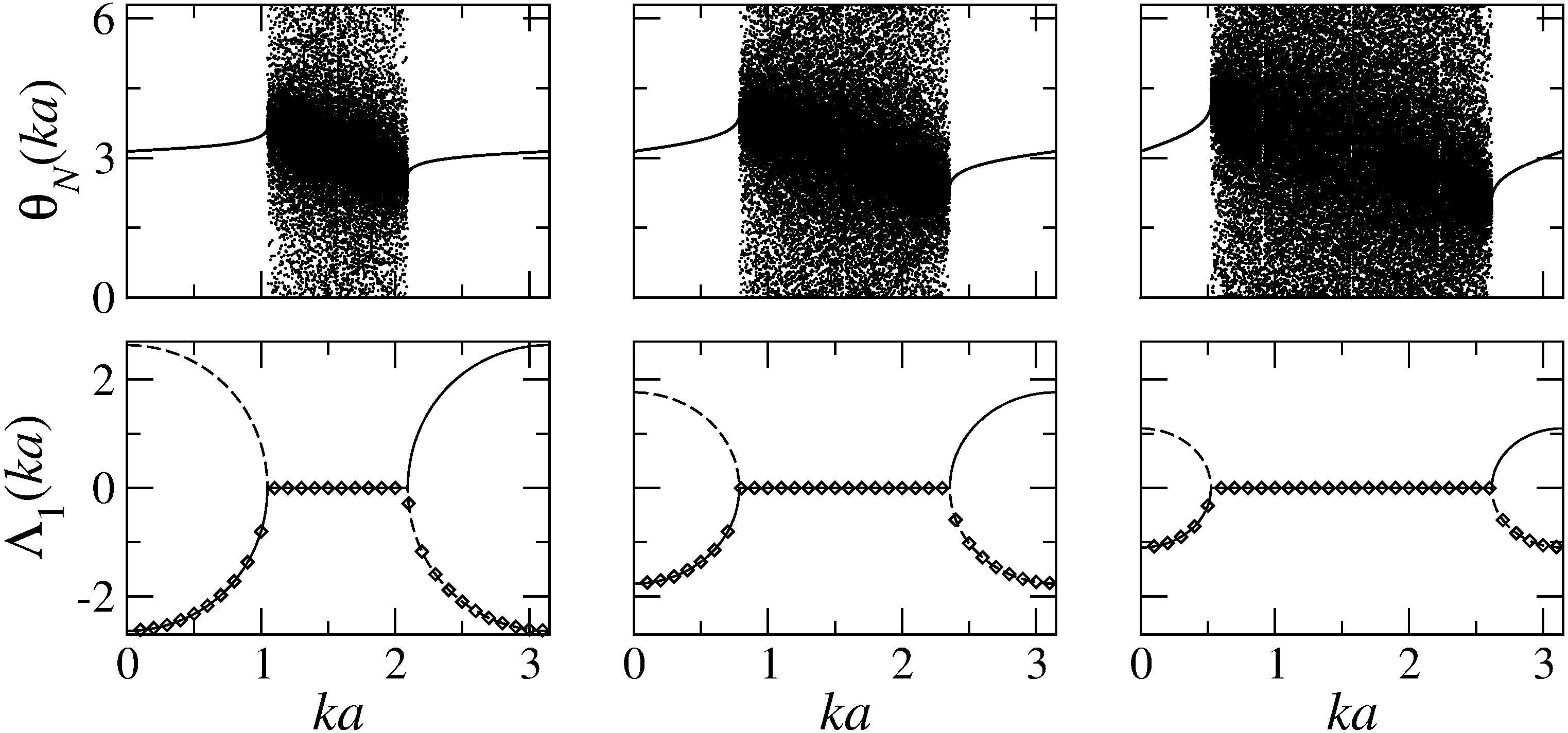
Figure 2: Upper panels: Bifurcation diagrams for a double Cayley tree of connectivity $K=1$ (left), $K=2$ (middle) and $K=3$ (right). For each value of $ka$ we plot only the last 50 iterations of $N=1000$ starting with an initial condition $\theta_{0}=0$. Lower panels: Finite $N$ Lyapunov coefficient. The diamonds correspond to the iteration $N=1000$ of Eq. (20), with an initial condition $\theta_{0}=0$. Continuous and dashed lines represent the Lyapunov coefficient (22) for the two roots of Eq. (14). For all cases $S_{12}=1/2$ and $S_{11}=-\sqrt{1-K/4}$.

II.3 Sensitivity to initial conditions

The dynamics of the map (13) is characterized by the sensitivity to initial conditions. For finite $N$, it is defined by MM-R

$$\Xi_{N}\equiv\mathrm{e}^{N\Lambda_{1}(N)}\equiv\left|\frac{\mathrm{d}\theta_{N}}{\mathrm{d}\theta_{0}}\right|,$$ (19)

where $\theta_{0}$ is the initial condition and $\Lambda_{1}(N)$ is the finite $N$ Lyapunov exponent. From Eq. (13), we find the following recursive relation for $\Xi_{N}$,

$$\Xi_{N}(ka)=\frac{K|S_{12}|^{4}}{\left|S^{*}_{12}\mathrm{e}^{-\mathrm{i}ka}+S^{*}_{11}S_{12}\mathrm{e}^{\mathrm{i}ka}\mathrm{e}^{\mathrm{i}\theta_{N-1}(ka)}\right|^{2}}\,\Xi_{N-1}(ka).$$ (20)

In the limit $N\to\infty$, $\Xi_{N}\to\xi_{N}$ with $\xi_{N}$ being the sensitivity to initial conditions, defined by

$$\xi_{N}(ka)=\mathrm{e}^{N\lambda_{1}(ka)},N\gg 1,$$ (21)

with $\lambda_{1}(ka)$ the Lyapunov exponent

$$\lambda_{1}(ka)=\ln\frac{K|S_{12}|^{4}}{\left|S^{*}_{12}\mathrm{e}^{-\mathrm{i}ka}+S^{*}_{11}S_{12}\mathrm{e}^{\mathrm{i}ka}\mathrm{e}^{\mathrm{i}\theta_{\infty}(ka)}\right|^{2}}.$$ (22)

In the lower panels of Fig. 2 we show the behavior of $\lambda_{1}(ka)$ (or $\Lambda_{1}(ka)$ in the limit $N\gg 1$) for the three cases: $K=1$, 2 and 3. We observe that in the windows of periodicity 1 the theoretical result $\lambda_{1}(ka)$ of Eq. (22) shows two values for a given $ka$, which correspond to both roots expressed in Eq. (14). For the repulsor, $\lambda_{1}(ka)>0$ indicating that $\xi_{N}(ka)$ diverges exponentially, while at the attractor $\lambda_{1}(ka)<0$ and $\xi_{N}(ka)$ decays exponentially with a typical length scale given by

$$\zeta_{1}(ka)=\frac{a}{|\lambda_{1}(ka)|}.$$ (23)

As it happens for the fixed-point solutions, only the solution for the attractor agrees with the $\Lambda_{1}(ka)$ obtained from the iteration of Eq. (20). For the ergodic windows we have $\lambda_{1}(ka)=0$, so nothing we can say about the $N$-dependence of $\xi_{N}(ka)$. However, in those windows $\Xi_{N}(ka)$ oscillates (not shown here) with $N$.

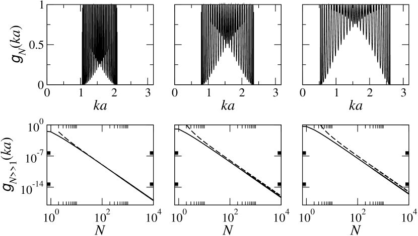
Figure 3: Upper panels: Bands of the dimensionless conductance for a double Cayley tree of connectivity $K=1$ (left), $K=2$ (middle), and $K=3$ (right), for $N=30$ and initial conditions $\theta_{0}=0$ and $\theta^{\prime}_{0}=\pi$. Lower panels: Dimensionless conductance at the critical attractors for $N\gg 1$ at $k_{c}a=\pi/3$ for $K=1$, $k_{c}a=\pi/4$ for $K=2$, and $k_{c}a=\pi/6$ for $K=3$. Dashed lines represent the theoretical result of Eq. (30) with $S_{12}=1/2$ and $S_{11}=-\sqrt{1-K/4}$.

At the critical attractors (those for the tangent bifurcations) we find that

$$\theta_{N}-\theta_{c}=(\theta_{N-1}-\theta_{c})\pm\sqrt{\frac{R_{\rm{node}}}{T_{\rm{node}}}}\left|\theta_{N-1}-\theta_{c}\right|^{2}+\cdots.$$ (24)

This local nonlinearity leads, via the functional composition renormalization group fixed-point map Schuster , to a $q$-exponential expression for the sensitivity for any $N$, namely Baldovin

$$\xi_{N}=\left(1-\frac{1}{2}\lambda_{3/2}N\right)^{-2},$$ (25)

where $\lambda_{3/2}$ is the $q$-generalized Lyapunov coefficient for $q=3/2$, which is given by $\lambda_{3/2}=\pm 2\sqrt{R_{\rm{node}}/T_{\rm{node}}}$. The plus and minus signs corresponds to trajectories at the left and right of the point of tangency $\theta_{c}$. When $\theta_{N}-\theta_{c}>0$, $\xi_{N}$ grows with $N$ faster than exponential and when $\theta_{N-1}-\theta_{c}<0$, $\xi_{N}$ decays with $N$ with a power-law behaviour, the typical decay length being given by

$$\zeta_{3/2}=\frac{a}{|\lambda_{3/2}|}=\frac{a}{2}\sqrt{\frac{T_{\rm{node}}}{R_{\rm{node}}}}.$$ (26)

This result on diverging duration of the laminar episodes of intermittency and large $N$ intervals of vanishing $\Xi_{N}$ between increasingly large spike oscillations.

III Consequences for the electronic transport

According to the Landauer formula, the dimensionless conductance $g_{{}_{N}}$ at the generation $N$ (conductance $G_{N}$ in units of $2e^{2}/h$) is just the transmission coefficient $|t_{N}|^{2}$ Buttiker . Using Eqs. (11) and (12) we find a recursion relation for the conductance, namely

$$g_{{}_{N}}(ka)=g_{{}_{N-1}}(ka)\,\frac{\Xi_{N}(ka)}{\Xi_{N-1}(ka)}\,\frac{\Xi^{\prime}_{N}(ka)}{\Xi^{\prime}_{N-1}(ka)}.$$ (27)

By iteration of this recursion relation we obtain

$$g_{{}_{N}}(ka)=\Xi_{N}(ka)\,\Xi^{\prime}_{N}(ka).$$ (28)

For the initial conditions $\theta_{0}=0$ and $\theta^{\prime}_{0}=\pi$, $\Lambda_{1}\to\lambda_{1}$ and $\Lambda^{\prime}_{1}\to\lambda_{1}$ for $N\gg 1$, therefore

$$g_{{}_{N}}(ka)=\mathrm{e}^{2N\lambda_{1}(ka)}.$$ (29)

This means that in the ergodic windows, where $\lambda_{1}(ka)=0$, the conductance does not decay but oscillates with $N$. However, in the windows of periodicity 1 $\lambda_{1}(ka)<0$ and $g_{{}_{N}}(ka)$ shows an exponential decay with $N$, whose typical length scale is $\zeta_{1}(ka)$ of Eq. (23). In analogy to the scaling behaviour of the conductance with the size of a disordered system Lee ; Beenakker , we name $\zeta_{1}(ka)$ localization length. In the upper panels of Fig. 3 we observe the bands of the dimensionless conductance, where the windows of periodicity 1 correspond to forbidden bands, while the chaotic windows relate to allowed bands. Critical attractors also correspond to the band edges, at which we expect that

$$g_{{}_{N}}=\xi_{N}^{2}=\left(1-\frac{1}{2}\lambda_{3/2}N\right)^{-4}.$$ (30)

That is, the conductance shows a power law decay, such that $\zeta_{3/2}$, in Eq. (26), is the typical decay length over large $N$ intervals located between increasingly large spike oscillations. In analogy with $\zeta_{1}$ we define $\zeta_{3/2}$ to be a localization length too. What is interesting about this length scale is its relation with the mean free path $\ell$ defined as Mello

$$\frac{1}{\ell}=\frac{1}{a}\,\cdot\,\frac{R_{\rm{node}}}{1-R_{\rm{node}}}.$$ (31)

This implies that the localization length at the critical attractors is one half of the geometric mean of the mean free path and the lattice constant,

$$\zeta_{3/2}=\frac{1}{2}\,\sqrt{\ell\,a},$$ (32)

which can be interpreted as the distance traveled by an electron before scattering. In the lower panels of Fig. 3 we observe that the power law decay fits very well with the scaling behavior with $N$ of the conductance.

IV Conclusions

We presented a generalized approach for the determination the dimensionless conductance of a double Cayley tree of charge scatterers of arbitrary connectivity. This is done by studying its scattering properties, as a function of the system size (generation), through the sensitivity to initial conditions of the nonlinear map satisfied by the eigenphases of the scattering matrix associated with the system. In the limit of a very large system the conducting and insulating bands correspond, respectively, to marginally chaotic windows and windows of periodicity 1. While in the conducting bands the conductance oscillates with the system size, in the insulating phase it displays an exponential decay with the system size, with a typical length scale, as in the scaling theory of localization. However, at the transition, on a band edge, when the conductance decays as a power law, the typical length scale is a $q$-generalized localization length, which is the geometric mean of the mean free path and the lattice constant.

The insulator to conductor transition in electronic transport systems is a condensed-matter phenomenon that still poses significant challenges before unabridged understanding is attained. The occurrence of a robust analogy between the size-dependent properties of an idealized network model of electron scatterers and the dynamical properties of a low-dimensional nonlinear map displaying tangent bifurcations is a remarkable finding. On the one hand this connection makes possible an exact determination of the conductance at the transition, while on the other hand reveals how a system composed of many degrees of freedom can undergo a drastic simplification.

V Acknowledgement

V. Domínguez-Rocha thanks DGAPA, UNAM, Mexico, for financial support. M. Martínez-Mares is grateful to the Sistema Nacional de Investigadores, Mexico. A. Robledo acknowledges support from DGAPA-UNAM-IN103814 and CONACyT-CB-2011-167978 (Mexican Agencies).

References

- (1) M. Martínez-Mares, A. Robledo, Phys. Rev. E 80, 045201(R) (2009).
- (2) Y. Jiang, M. Martínez-Mares, E. Castaño, A. Robledo, Phys. Rev. E 85, 057202 (2012).
- (3) V. Domínguez-Rocha, M. Martínez-Mares, J. Phys. A: Math. Theor. 46, 235101 (2013).
- (4) H.G. Schuster, Deterministic Chaos. An Introduction (VCH Publishers, Weinheim, 1988).
- (5) A. Wolf, J.B. Swift, H.L. Swinney, J.A. Vastano, Physica D 16, 285 (1985).
- (6) F. Baldovin, A. Robledo, Europhys. Lett. 60, 518 (2002).
- (7) M. Büttiker, IBM J. Res. Dev. 32, 317 (1988).
- (8) P.A. Lee, T.V. Ramakrishnan, Rev. Mod. Phys. 57, 287 (1985).
- (9) C.W.J. Beenakker, Rev. Mod. Phys. 69, 731 (1997).
- (10) P.A. Mello, N. Kumar, Quantum Transport in Mesoscopic Systems. Complexity and Statistical Fluctuations (Oxford University Press, New York, 2004) p. 289