Using Neural Networks to Compute Approximate and Guaranteed Feasible Hamilton-Jacobi-Bellman PDE Solutions

Abstract

To sidestep the curse of dimensionality when computing solutions to Hamilton-Jacobi-Bellman partial differential equations (HJB PDE), we propose an algorithm that leverages a neural network to approximate the value function. We show that our final approximation of the value function generates near optimal controls which are guaranteed to successfully drive the system to a target state. Our framework is not dependent on state space discretization, leading to a significant reduction in computation time and space complexity in comparison with dynamic programming-based approaches. Using this grid-free approach also enables us to plan over longer time horizons with relatively little additional computation overhead. Unlike many previous neural network HJB PDE approximating formulations, our approximation is strictly conservative and hence any trajectories we generate will be strictly feasible. For demonstration, we specialize our new general framework to the Dubins car model and discuss how the framework can be applied to other models with higher-dimensional state spaces.

I Introduction

In recent years, rapid progress in robotics and artificial intelligence has accelerated the need for efficient path-planning algorithms in high-dimensional spaces. In particular, there has been vast interest in the development of autonomous cars and unmanned aerial vehicles (UAVs) for civilian purposes [1, 2, 3, 4, 5, 6]. As such systems grow in complexity, development of algorithms that can tractably control them in high-dimensional state spaces are becoming necessary.

Many path planning problems can be cast as optimal control problems with initial and final state constraints. Dynamic programming-based methods for optimal control recursively compute controls using the Hamilton-Jacobi-Bellman (HJB) partial differential equation (PDE). Such methods suffer from space and time complexities that scale exponentially with the system dimension. Dynamic programming is also the backbone for Hamilton-Jacobi (HJ) reachability analysis, which solves a specific type of optimal control problem and is a theoretically important and practically powerful tool for analyzing a large range of systems. It has been extensively studied in [7, 8, 9, 10, 11, 12, 13, 14], and successfully applied to many low-dimensional real world systems [15, 16, 11]. We use the reachability framework to validate our method.

To alleviate the curse of dimensionality, many proposed dynamic programming-based methods heavily restrict the system at hand [17, 18, 19]. Other less restrictive methods use projections, approximate dynamic programming, and approximate systems decoupling [20, 21, 22], each limited in flexibility, scalability, and degree of conservatism. There are also several approaches towards scalable verification [23, 24, 25, 26]; however, to the best of our knowledge, these methods do not extend easily to control synthesis. Direct and indirect methods for optimal control, such as nonlinear model predictive control [27], the calculus of variations [28], and shooting methods [29], avoid dynamic programming altogether but bring about other issues such as nonlinearity, instability, and sensitivity to initial conditions.

One primary drawback of dynamic programming-based approaches is the need to compute a value function over a large portion of the state space. This is computationally wasteful since the value function, from which the optimal controller is derived, is only needed along a trajectory from the system’s initial state to the target set. A more efficient approach would be to only compute the value function local to the trajectory from the initial state to the target set. However, there is no way of knowing where such a trajectory will lie before thoroughly computing the value function.

Methods that exploit machine learning have great potential because they are state discretization-free and do not depend on the dynamic programming principle. Unfortunately, many machine learning techniques cannot make the guarantees provided by reachability analysis. For instance, [30] and [31] use neural networks (NNs) as nonlinear optimizers to synthesize trajectories which may not be dynamically feasible. The authors in [32] propose a supervised learning-based algorithm that depends heavily on feature tuning and design, making its application to high-dimensional problems cumbersome. In [33] and [34], the authors successfully use NNs for approximating the value function, but the approximation is not guaranteed to be conservative.

In this paper, we attempt to combine the best features of both dynamic programming-based optimal control and machine learning using an NN-based algorithm. Our proposed grid-free method conservatively approximates the value function in only a region around a feasible trajectory. Unlike previous machine learning techniques, our technique guarantees a direction of conservatism, and unlike previous dynamic programming-based methods, our approach involves an NN that effectively finds the relevant region that requires a value function. Our contributions will be presented as follows:

• In Section II, we summarize optimal control and the formalisms used for this work.

• In Section III, we provide an overview of the full method and the core ideas behind each stage, as well as highlight the conservative guarantees of the method.

• In Sections IV and V, we present the two phases of our proposed algorithm and the underlying design choices.

• In Section VI, we illustrate our guaranteed-conservative approximation of the value function, and the resulting near-optimal trajectories for the Dubins Car.

• In Section VII, we conclude and discuss future directions.

II Problem Formulation

In this section, we will provide some definitions essential to express our main results. Afterwards, we will briefly discuss the goals of this paper.

II-A Optimal Control Problem

Consider a dynamical system governed by the following ordinary differential equation (ODE):

$$\dot{x}=f(x,u),t\in[t_{0},0]$$ (1)

$$x(t_{0})=\bar{x},\quad u\in\mathcal{U}$$

Note that since the system dynamics (1) is time-invariant, we assume without loss of generality that the final time is $0$.

Here, $x\in\mathbb{R}^{n}$ is the state of the system and the control function $u(\cdot)$ is assumed to be drawn from the set of measurable functions. Let us further assume that the system dynamics $f:\mathbb{R}^{n}\times\mathcal{U}\rightarrow\mathbb{R}^{n}$ are uniformly continuous, bounded, and Lipschitz continuous in $x$ for fixed $u$. Denote the function space from which $f$ is drawn as $\mathbb{F}$.

With these assumptions, given some initial state $x$, initial time $t_{0}$, and control function $u(\cdot)\in\mathbb{U}$, there exists a unique trajectory solving (1). We refer to trajectories of (1) starting from state $x_{1}$ and time $t_{1}$ as $\xi^{f}(t;x_{1},t_{1},u(\cdot))$, with $x_{1}\in\mathbb{R}^{n}$ and $t_{0}\leq t,t_{1}\leq 0$. Trajectories satisfy an initial condition and (1) almost everywhere:

$$\frac{d}{dt}\xi^{f}(t;x_{1},t_{1},u(\cdot))=f(\xi^{f}(t;x_{1},t_{1},u(\cdot)),u(t))$$ (2)

$$\xi^{f}(t_{1};x_{1},t_{1},u(\cdot))=x_{1}$$

Note that we can use the trajectory notation to specify states that satisfy a final condition if $t\leq t_{1}$. In this paper this will often be the case, since our NN will be producing backward-time trajectories.

Consider the following optimal control problem with final state constraint:

$$V(x,t)=\min_{u(\cdot),t_{0}}\int_{t}^{0}C(u(\tau))d\tau$$ (3)

$$\text{subject to }x(t_{0})=\bar{x},x(0)=x_{\mathcal{L}}$$

The value function $V(x,t)$ is typically obtained via dynamic programming-based approaches such as [35, 11, 13, 14, 36, 37, 38, 39], and an appropriate HJB partial differential equation is solved backwards in time on a grid representing the discretization of states. Once $V(x,t)$ is found, the optimal control, which we denote $u^{*}(x,t)$, can be computed based on the gradient of $V(x,t)$:

$$u^{*}(x,t)=\arg\min_{u\in\mathcal{U}}\nabla V(x,t)\cdot f(x,u)$$ (4)

Unfortunately, the computational complexity of these methods scales exponentially with the state space dimension.

II-B Goal

In this paper, we seek to overcome the exponentially scaling computational complexity. Our approach is inspired by two inherent challenges that dynamic programming-based methods face. First, since only relatively mild assumptions are placed on the system dynamics (1), optimal trajectories are a priori unknown and could essentially trace out any arbitrary path in the state space. Dynamic programming ignores this issue by considering all possible trajectories. Second, in a practical setting, the system starts at some particular state $x_{0}$. Thus, the optimal control, and in particular $\nabla V(x,t)$ in (4), is needed only in a “corridor” along the optimal trajectory. However, since the optimal trajectory is a priori unknown, dynamic programming-based approaches resort to computing $V(x,t)$ over a very large portion of the state space so that the $\nabla V(x,t)$ is available regardless of where the optimal trajectory happens to be.

In this paper, we propose a method that, in contrast to dynamic programming-based methods,

1. has a substantially faster computation time and smaller memory-usage;

2. is a flexible and general framework that can be applied to higher-order systems with just hyperparameter tuning;

3. generates an approximate value function $\hat{V}(x,t)$ from which a controller that drives the system to the target can be synthesized;

4. guarantees that $\hat{V}(x,t)\geq V(x,t)~{}\forall x,t$, so that a direction of conservatism can be maintained despite the use of an NN.

We enforce 1) by avoiding operations that exhaustively search the state space. As seen in Section IV-B, the training and final data sets are either generated randomly or outputted by the NN, both constant time operations. Furthermore, we rely on NNs being universal function approximators [40] to make our method general to the system dynamics, thus satisfying 2). While our method does have some limitations, as discussed at the end of Section IV-A, we do not believe that these limitations are restrictive in the context of optimal control. Our post-processing of the NN outputs outlined in Section V satisfies 3). Finally, we use the dynamics of the system to ensure our final output satisfies 4); this is detailed in Section IV-B.

Our method overcomes the challenges faced by dynamic programming-based methods in two phases: the NN training phase, which allows the NN to learn the inverse backward system dynamics while also generating a dataset from which we can obtain a conservative approximation of the value function; and the controller synthesis phase, which uses the approximation to synthesize a controller to drive the system from its initial state to its target.

III Overview

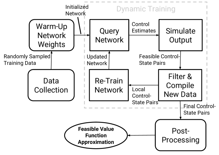
Figure 1: Stages of proposed method

In this section we will briefly describe the different stages of our computational framework (depicted in Fig. 1). We leave the details of each stage to subsections of Section IV and V.

III-A Pre-Training

In the pre-training phase (detailed in Section IV-B1), we produce some initial datasets to prepare the NN for the dynamic training procedure. The dynamic training procedure is already designed to help the NN improve its performance iteratively; however, the pre-training phase speeds up the convergence by warming up the NN with sampled data of the system dynamics, $f$.

III-B Dynamic Training

Our proposed dynamic training loop is tasked with both improving the approximation of the NN and producing the necessary data from which we extract our value function approximation. Fortunately, these two tasks are inherently tied to one another.

We pose our NN as an approximation of the inverse dynamics of the system (this is formally clarified in Section IV). In other words, if we query our NN with a set of states to check its approximation, then the NN will predict a set of controls to drive the system to those states (detailed in Section IV-B2). We can check the correctness of this prediction by simulating the controls through $f$ (detailed in Section IV-B3). Even if this prediction is inaccurate, we can recycle the new data the NN produced through an attempted prediction, and add the data into our training set to re-train the NN. Since we simulated the NN’s prediction to get the actual states the predicted control drives the system to, we now have corrective data with which we can re-train our NN. By doing this repeatedly, we iteratively train the NN with feedback. The data produced by the NN can be used to evaluate an approximate value of the value function using (3). Thus, with this dynamic training loop, we are able to produce data to construct an approximate value function while iteratively improving our NN’s prediction capabilities. Furthermore, as the NN improves, the relevance of the data also improves.

To further encourage the process, in every iteration we additionally apply stochastic filters to our dataset that favor more local and optimal data (detailed in Section IV-B4). This way, we can ensure the NN will not saturate or keep any unnecessary data for our final value function approximation.

III-C Post-Training

Once dynamic training is complete, the NN will be able to make accurate predictions and our dataset will encompass the region over which an approximate value function is needed. After some post-processing over the dataset (detailed in Section IV-C), we will show that we can successfully extract a value function approximation from which we synthesize control to drive our system from our initial state to our goal state.

IV Neural Network Training Phase

Given a target state $x_{\mathcal{L}}$ and assuming the system starts at some initial state $\bar{x}$, we want to design an NN that can produce a control function $u(\cdot)$ that drives the backward-time system from $x_{\mathcal{L}}$ to $\bar{x}$. More concretely, consider the inverse backward dynamics of the system, denoted $g_{{x_{\mathcal{L}}}}:\mathbb{R}^{n}\times\mathbb{F}\rightarrow\mathbb{U}$, and defined to be

$$g_{x_{\mathcal{L}}}(\bar{x};-f(\cdot,\cdot))=u^{*}(\cdot)\\$$ (5)

where the optimal control $u^{*}(\cdot)$ is defined for $t\leq 0$. For simplicity, we will write $g_{x_{\mathcal{L}}}$ as $g$ from now on. Given some $u^{*}(\cdot)$ defined in the time interval $[t,0]$, we have $\bar{x}=\xi^{f}(0;x_{\mathcal{L}},t,u^{*}(\cdot))$.

Our NN is an approximation of $g$, and we will denote the NN as $\hat{g}$. Let $\hat{u}(\cdot)$ be the control produced by $\hat{g}$, and let the time interval for which $\hat{u}(\cdot)$ is defined be denoted $[-\hat{T},0]$. The primary tasks of our training procedure will be to:

1. iteratively improve our NN’s training set so $\hat{g}$ approaches $g$ in the region local to the path given by $\xi^{f}(0;x_{\mathcal{L}},t,u^{*}(\cdot)),t\leq 0$; and

2. produce a dataset of states, their corresponding control and, in turn, the corresponding value approximation, which will be used for control synthesis.

IV-A Neural Network Architecture

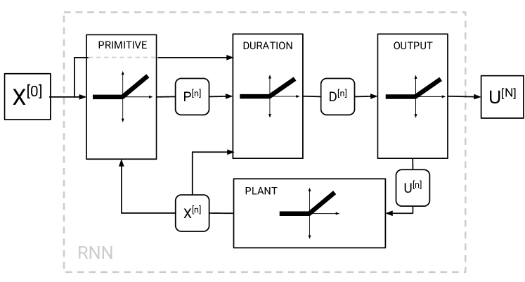
Figure 2: Four-layer RNN which takes input states and outputs discretized control.

Denote the maximum time horizon as $\bar{T}$. To reduce the space in which the NN needs to look for candidate control functions, we assume that $\hat{u}(\cdot)$ returned by the NN is composed of two finite sequences $\{u^{j}\}_{j=1}^{K},\{\tau^{j}\}_{j=1}^{K}$ called the sequence of control primitives and the sequence of time durations respectively. Mathematically, the control function $\hat{u}(\cdot)$ is of the form

$$\hat{u}(t)=\begin{cases}u^{1},&\quad t\in[-\sum_{j=1}^{K}\tau^{j},-\sum_{j=2}^{K}\tau^{j}]\\ u^{2},&\quad t\in(-\sum_{j=2}^{K}\tau^{j},-\sum_{j=3}^{K}\tau^{j}]\\ \cdots&\\ u^{K-1},&\quad t\in\left(-\tau^{K}-\tau^{K-1},-\tau^{K}\right]\\ u^{K},&\quad t\in\left(-\tau^{K},0\right]\\ \end{cases}$$ (6)

where we implicitly define $\hat{T}=\sum_{j=1}^{K}\tau^{j}$. Since we will only use the control to obtain the approximation $\hat{V}(\cdot,\cdot)$ and not for actually controlling the system, we do not need the generated controls to be extremely accurate or continuous, as we will explain in Sections IV-B and V.

We propose a rectified linear unit recurrent NN (RNN) with the following structure:

Primitive Layer: $$P^{[n]}=\psi(W_{P}\cdot X^{[n]}+b_{P})$$

Duration Layer: $$D^{[n]}=\psi(W_{D_{1}}\cdot P^{[n]}+W_{D_{2}}\cdot X^{[n]}+b_{D})$$

Control Layer: $$U^{[n]}=W_{L}\cdot D^{[n]}+b_{L}$$

Plant Layer: $$X^{[n+1]}=\psi(W_{X}\cdot U^{[n]}+b_{X})$$

where $\psi$ is the positive rectifying function defined as $\psi(a)=\max(0,a)$ and $n=0,1,\ldots,N$. The input of the RNN is $\bar{x}$ ($X^{[0]}=\bar{x}$), and the output is some $\hat{u}(\cdot)$ ($U^{[N]}=\hat{u}(\cdot)$), that approximately brings the system from $\bar{x}$ to $x_{\mathcal{L}}$. The parameters we learn through training are the weights $W_{P}$, $W_{D_{1}}$, $W_{D_{2}}$, $W_{L}$, $W_{X}$ and biases $b_{P},b_{D},b_{L},b_{X}$. All weights and biases will be collectively denoted $\mathbb{W}$. For prediction, $\hat{u}(\cdot)$ and training example, $u(\cdot)$, we discretize both controls using (6), then the training is performed with mean-squared error (MSE), or

$$MSE=\frac{1}{n}\sum_{n=1}^{N}(\hat{u}^{n}-u^{n})^{2}$$ (7)

as the cost function, where $u(\cdot)$ is our training example output.

As already mentioned, the primitive layer takes a state as input and computes a control primitive. The duration layer takes in the primitive layer’s output and the same input state, and outputs a time duration. This time duration is then passed through the control (also called output) linear layer, which outputs the sequences $\{u^{j}\},\{\tau^{j}\}$ representing the control function $\hat{u}(\cdot)$. Afterwards, the control function is fed into the plant layer, which attempts to encode the backward dynamics $-f$. The plant’s output state, $X^{[n+1]}$, is then fed back to the primitive layer.

Explicitly, the RNN can be written as

$$\hat{g}(\bar{x},x_{\mathcal{L}};-f(\cdot,\cdot),\mathbb{W})=\hat{u}(\cdot)=U^{[N]}$$ (8)

where $\hat{u}(\cdot)$ is given in the form of the sequences $\{u^{j}\},\{\tau^{j}\}$.

In the next section, we discuss the dynamic training procedure for this RNN.

IV-B Detailed Dynamic Training

IV-B1 Warm-up and Initial Training

We first train the RNN without knowledge of $\bar{x}$. For starters, we will require training examples in the form of $\{\hat{x}_{i},\hat{u}_{i}(\cdot)\}$ that sufficiently capture the basic behaviors of the system dynamics. To do this, we randomly generate $\{\hat{x}_{i}\}$ using an accept-reject algorithm similar to the one in [33], which is described in Alg. 1.

Algorithm 1 Exponential Filter

1:  Result: $A$

2:  Inputs: $x$, $\mathcal{R}$, $\lambda$

3:  compute $x_{\text{proj}}$ via (9)

4:  generate $\beta$ uniformly from $[0,\lambda]$ 

5:  if $x\in\mathcal{R}$ then

6:     $A$ = true 

7:  else

8:     if $\beta\leq\lambda e^{-\lambda\|x-x_{\textrm{proj}}\|_{2}}$  then

9:        $A=$ true 

10:     else

11:        $A=$ false 

12:     end if

13:  end if

Algorithm 2 Length Filter

1:  Result: $\mathcal{\mathcal{X}}$

2:  Inputs: $\mathcal{X}$, $\lambda_{C}$, $\hat{C}(\mathcal{X})$, $D$

3:  generate $\beta$ uniformly from $[0,\lambda]$ 

4:  for $x_{i}\in\mathcal{X}$ do

5:     $\mathcal{X}_{C}\leftarrow\emptyset$ 

6:     for $x_{j}\neq x_{i}\in\mathcal{X}:||x_{i}-x_{j}||_{2}\leq D$ do

7:        if $\beta>\lambda_{C}e^{-\lambda_{C}\hat{C}(x_{j})}$  then

8:           $\mathcal{X}_{C}\leftarrow\mathcal{X}_{C}\cup x_{j}$ 

9:        end if

10:     end for

11:     $\mathcal{X}\leftarrow\mathcal{X}\setminus\mathcal{X}_{C}$  

12:  end for

Alg. 1 takes a state $x$, an accept region $\mathcal{R}$, and a decay rate $\lambda$ as inputs. To use Alg. 1, we first compute $x_{\text{proj}}$, the Euclidean projection of the state $x$ onto the set $\mathcal{R}$ as follows:

$$x_{\text{proj}}=\arg\min_{x^{\prime}}\|x^{\prime}-x\|_{2}:x^{\prime}\in\mathcal{R}$$ (9)

Using Alg. 1, we generate two training sets: one large dataset $\mathcal{D}_{1}$ and one small dataset $\mathcal{D}_{2}$. The large data set $\mathcal{D}_{1}$, used for supervised training of the plant layer (the weights $W_{X}$), is generated with a large accept region with a large number of accepted points. The smaller dataset $\mathcal{D}_{2}$, used to initialize the full RNN after the plant layer has been warmed up with $\mathcal{D}_{1}$, is generated with a smaller accept region and a relatively small number of accepted points.

Once the RNN’s plant layer is warmed up with $\mathcal{D}_{1}$ and the full network has been trained on $\mathcal{D}_{2}$, the RNN is ready to be queried, setting the dynamic training loop into motion.

IV-B2 Neural Network Query

At the start of every training loop, the RNN is used to predict controls, $\{\hat{u}_{i}(\cdot)\}_{i=1}^{N}$, from a set of states $\{\bar{x}_{i}\}_{i=1}^{N}$.

For our training loop’s first query, we uniformly sample $M_{\epsilon}$ states within a distance of $\epsilon$ to $\bar{x}$ to produce a set of states denoted $\mathcal{X}_{\epsilon}=\{\bar{x}_{i}\}_{i=1}^{M_{\epsilon}}$. Then, for all of the network queries, we query the RNN with the same $\mathcal{X}_{\epsilon}$ to get its current set of predictions, $\mathcal{V}_{\epsilon}=\{\hat{u}_{i}(\cdot)\}_{i=1}^{M_{\epsilon}}$. By using a set of states, $\mathcal{X}_{\epsilon}$, as opposed to using just a singular state, we capture more local trajectories and relax the need for every trajectory to lead exactly to a point location in the state space.

IV-B3 Simulate Output and Feasibility

In general, applying a control in $\mathcal{V}_{\epsilon}$ brings the backward system from $x_{\mathcal{L}}$ to some $\hat{x}\not\in\mathcal{X}_{\epsilon}$. Thus, to find $\mathcal{V}_{\epsilon}$’s true set of resultant states, we simply apply each control in $\mathcal{V}\epsilon$ to $f$ with $x_{\mathcal{L}}$ as the initial condition. This will yield $\mathcal{V}_{\epsilon}$’s true set of resultant states, which we denote as $\mathcal{X}_{\epsilon}^{\prime}$.

This key step is what gives us our feasibilty guarantee. Since all of the data in our final output is a compilation of filtered data drawn from $(\mathcal{X}_{\epsilon}^{\prime},\mathcal{V}_{\epsilon})$ at each training cycle, we know we have a dynamically feasible control for each state. In addition, since the controls are feasible, they must also be either optimal or suboptimal. Therefore, when we compute values from our final set of controls using (3), these values must be strictly conservative.

IV-B4 Filtering

Often the RNN will predict a $\mathcal{V}_{\epsilon}$ that lead to states far from our target. Since our method is intended to produce a value function approximation local to a relevant region of the state space, we apply an exponential accept-reject filter (Alg. 1) to $\mathcal{X}^{\prime}_{\epsilon}$, with accept region $\mathcal{R}_{\epsilon}$ and decay rate $\lambda_{\epsilon}$, to stochastically remove states that are not nearby. We let the remaining states and their corresponding controls be $(\mathcal{X}_{\text{new}},\mathcal{V}_{\text{new}})$.

We choose the input accept region $\mathcal{R}_{\epsilon}$ and decay rate $\lambda_{\epsilon}$ provided to Alg. 1 such that the filter will generously accept states that could lie near a feasible path from $\bar{x}$ to $x_{\mathcal{L}}$. Though choosing a reasonable $\mathcal{R}_{\epsilon}$ for general high-dimensional systems with complicated dynamics before training could be difficult since we may be unable to provide even a generous guess of where in the state space optimal trajectories might lie, we can instead adjust the size or shape of $\mathcal{R}_{\epsilon}$ until the region begins accepting predictions from the RNN.

After finding $(\mathcal{X}_{\text{new}},\mathcal{V}_{\text{new}})$, we can update our full training set on which we will train our RNN, for the next training iteration. We first improve our current training set, denoted as $(\mathcal{X},\mathcal{V})$, by once again applying Alg. 1 with accept region $\mathcal{R}$ and decay rate $\lambda$. Then, we apply a second filter to all of our remaining data that favors controls with relatively low costs, this is detailed in Alg. 2 with inputs $\mathcal{X}$, the costs $\hat{C}(\mathcal{X})$, and decay rate $\lambda_{C}$ and search radius $D$. We let the remaining data set from filtering $(\mathcal{X},\mathcal{V})$ be called $(\mathcal{X}_{\text{old}},\mathcal{V}_{\text{old}})$. Then, we compile our new training set for the next training cycle as $(\mathcal{X},\mathcal{V})=(\{\mathcal{X}_{\text{old}},\mathcal{X}_{\text{new}}\},\{\mathcal{V}_{\text{old}},\mathcal{V}_{\text{new}}\})$.

IV-C Post-processing

In order to drive the system from $\bar{x}$ to $x_{\mathcal{L}}$, the value function, and in particular its gradient, is necessary at points between $\bar{x}$ and $x_{\mathcal{L}}$ along a dynamically feasible trajectory. Fortunately, this information can be computed from $\mathcal{X}$ and $\mathcal{V}$. Specifically, $\hat{x}_{i}\in\mathcal{X}$ and $\hat{u}_{i}(\cdot)\in\mathcal{V}$ produce a trajectory $\xi^{f}_{i}(0;\hat{x}_{i},t,\hat{u}_{i}(\cdot)),t\in[\hat{T},0]$. From the trajectories, we can obtain $M_{i}$ states on the trajectory by discretizing the time $t$ into $M_{i}$ points. We denote these states $x_{(i,j)}$, where the index $i$ comes from the index of $\hat{x}_{i}\in\mathcal{X}$, and the index $j\in\{0,\ldots,M_{i}-1\}$ indicates that the state is computed from the $j$th time point on the trajectory $\xi^{f}_{i}$. Mathematically, $\hat{x}_{(i,j)}$ is given as follows:

$$\hat{x}_{(i,j)}=\xi_{i}^{f}(0;\hat{x}_{i},t_{j},\hat{u}_{i}(\cdot)),$$ (10)

$$t_{j}=-\frac{j\hat{T}_{i}}{M_{i}-1},j=0,1,\ldots,M_{i}-1$$

Once we have explicitly added data along the trajectories from our dataset, we now have a dataset that spans the local state space around and between $\bar{x}$ and $x_{\mathcal{L}}$. To get our value function approximation across our dataset, we can simply use (3). Explicitly, for state-control pair, $(\hat{x}_{i},\hat{u}_{i}(\cdot))\in\mathcal{X}\times\mathcal{V}$, and $t_{j}$, we have the approximate value function at states $x_{(i,j))}$ and times $t_{j}$:

$$\hat{V}(x_{(i,j)},t_{j})=\int_{t_{j}}^{0}C(\hat{u}_{i}(t))dt$$ (11)

V Controller Synthesis Phase

After we obtain our value function approximation, we can synthesize control to drive our system from $\bar{x}$ to $x_{\mathcal{L}}$ using (4) with the appropriate gradient components of the value function. However, since our value function approximation is irregular and based in a point set, we will first define a special computation for obtaining the gradient.

To compute $(\nabla V)_{i}$, the $i$th component of the gradient at a given state $x$, we search above and below in the $\hat{i}$ direction for states in $\mathcal{X}$ within a hyper-cylinder of tunable radius $r$. We define the closest point within the hyper-cylinder above $x$ as $x_{a}$ and below as $x_{b}$. If some $x_{a}$ and $x_{b}$ exist, we compute the gradient at $x$ as:

$$(\nabla V(x))_{i}=\frac{V(x_{a})-V(x_{b})}{(x_{a})_{i}-x_{b})_{i}}$$ (12)

If we have multiple states above but none below, we approximate the gradient using (12), with $x_{a}$ being the closest state above and $x_{b}$ being the second closest state above. A similar procedure holds if we have multiple states below but none above.

In general, we can use a finite element method to compute gradient values for a non-regular grid, which involves using shape functions as basis functions to interpolate the gradient values between nodes.

VI Dubins Car Example

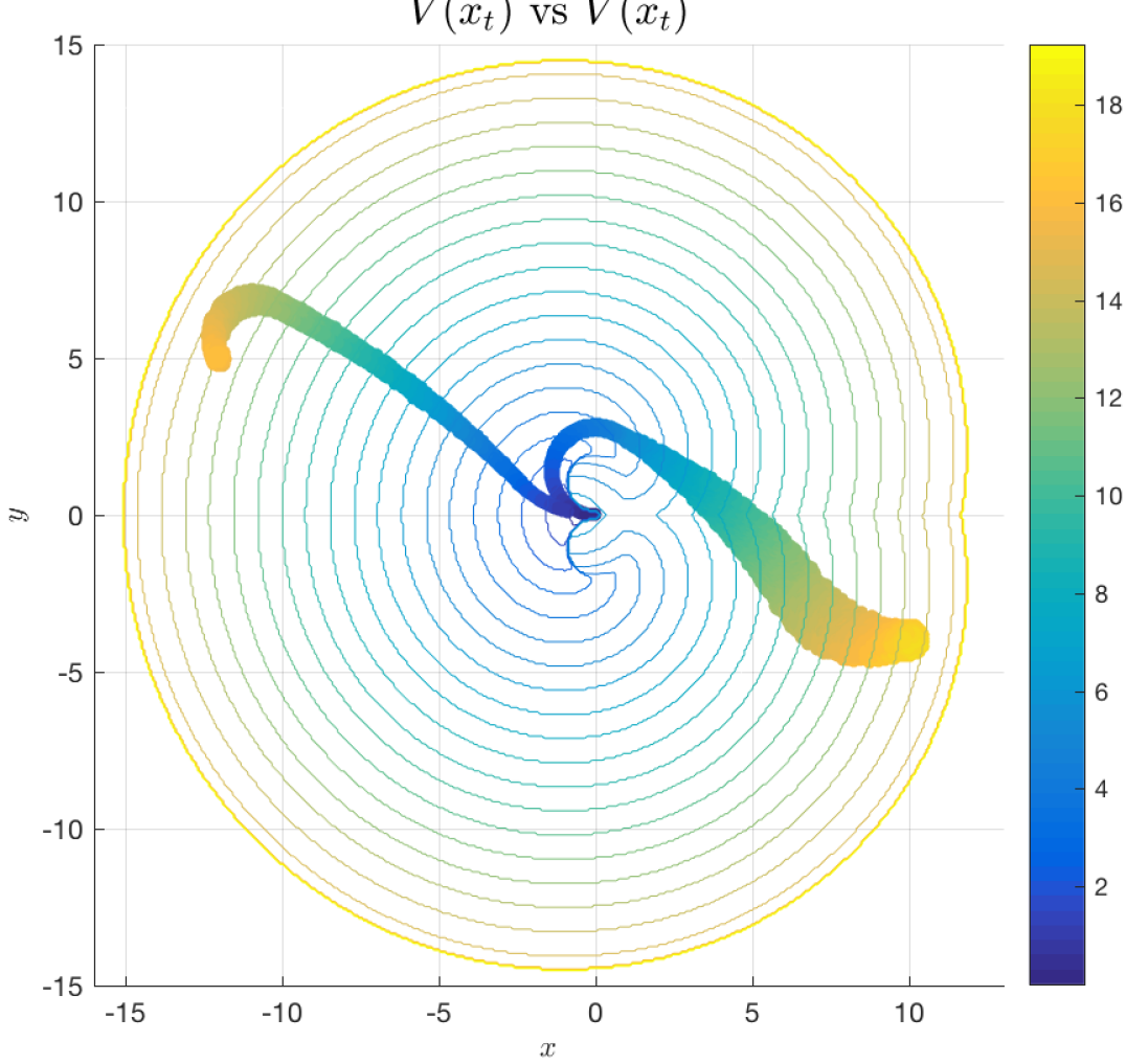
Figure 3: Comparison of the true value function $V(x,t_{0}^{*})$ computed over a large portion of the state space, and the approximate value function from our NN-based approach $\hat{V}(x_{(i,j)},t_{j})$ on two different corridors containing the initial state $\bar{x}$, the target set $x_{\mathcal{L}}$, and a dynamically feasible trajectory. The contours are level sets of $V(x,t_{0}^{*})$. Two different corridors in which $\hat{V}$ is computed resulting from two different values of $\bar{x}$ ($(10,-4,-3),(-12,5,2)$) are also plotted using the same colormap.

VI-A Vehicle Dynamics

Consider the Dubins Car [41], with state $x=(p_{x},p_{y},\theta)$. $(p_{x},p_{y})$ are the $x$ and $y$ positions of the vehicle, and $\theta$ is the heading of the vehicle. The system dynamics, assuming unit longitudinal speed, are

$$\dot{p}_{x}=\cos\theta, \ \dot{p}_{y}=\sin\theta$$ (13)

$$\dot{\theta} =u,\qquad|u|\leq 1$$

The control of the Dubins car is denoted $u$, and is constrained to lie in the interval $[-1,1]$, the interpretation of which is that the vehicle has a maximum turn rate of $1$ rad/s. In addition, we only accrue cost on our control with the duration of the control. Formally, this means that $C(u(t))=1$. We choose the Dubins car to illustrate our method because of the simple structure of the optimal controls. In addition, since the model is only 3D, we are able to verify our results by comparing them to the those obtained via HJ reachability.

For our example, we choose many different initial states $\bar{x}$ for the system. The target state $x_{\mathcal{L}}$ is chosen as the origin.

VI-B Control Primitives

In [41], Dubins shows that all optimal trajectories of this system utilize controls that represent going straight or turning maximally left or right. Thus, the set of controls that are valid for generating optimal trajectories can be reduced down to three motion primitives, {‘L’, ‘S’, ‘R’}, encoding the controls $u=1$ (max left), $u=0$ (straight), and $u=-1$ (max right) respectively. Though [41] additionally provides an algebraic solution to the optimal control problem, we purposefully do not leverage this result, as many interesting systems do not have such a simple method of deriving optimal control. Instead, we use five motion primitives, encoding the controls $u=2$, $u=1$, $u=0$, $u=-1$, $u=-2$.

Following our notation in Section IV, we write a $n$ length control sequence as $\{u^{1},u^{2},\ldots,u^{n}\},\{\tau^{1},\tau^{2},\ldots,\tau^{n}\}$ where $u^{i}$ denotes the $i$th control primitive and $\tau^{i}$ denotes the duration of $i$th control primitive.

VI-C Neural Network

Using the RNN architecture described in Section IV-A, we let $N=3$, since we only need at most three control primitives. Since the controls and dynamics of Dubins car are simple, we have chosen the number of neurons in layers $P,D,U,X$ to be $[10,10,6,75]$, respectively. The NN is trained with the training functionality of the MATLAB Neural Network ToolBox 2016a. The training function used for the full NN is resilient back-propagation and the performance function used is mean squared error.

VI-D Dynamic Training

For $\mathcal{D}_{1}$ and $\mathcal{D}_{2}$, we choose each $u^{i}$ from the three possible values $\{-1,0,1\}$. The controls for $\mathcal{D}_{1}$ have durations, $\tau^{i}$, uniformly sampled from $[0,\bar{T}]$ where $\bar{T}=100$. $\mathcal{D}_{2}$’s control durations are also uniformly sampled in the same manner, but with $\bar{T}=2\pi$.

For the dynamic training parameters, our query set $\mathcal{X}_{\epsilon}$ is generated with $\epsilon=1$ and $M_{\epsilon}=500$.

VI-D1 Filtering Algorithms

Throughout training, the exponential filtering process uses two accept regions. In early iterations, $\mathcal{R}=\mathcal{R}_{c}$ is defined as the cone of minimum size that contains $\mathcal{X}_{\epsilon}$, with the tip of the cone located at $\bar{x}$. The choice of using a conical filter to guide the neural net at first is based on the hypothesis that a trajectory taking the system from $\bar{x}$ to $x_{\mathcal{L}}$ is likely to stay in the cone $\mathcal{R}_{c}$. In later iterations, $\mathcal{R}=\mathcal{R}_{s}$ is chosen as $\mathcal{X}_{\epsilon}$. This spherical filter, centered at $x_{\mathcal{L}}$, helps to more finely guide the neural network to $x_{\mathcal{L}}$.

We also apply length filtering with a small distance parameter $D=0.5$, since we would like to be comparing distance costs only between trajectories with similar end points.

VI-D2 Filter Decay Rate: Setting and Timing

Although $\mathcal{R}_{\text{C}}$ and $\mathcal{R}_{\text{S}}$ are chosen before the dynamic training process, the filtering of the training set $\mathcal{X}$ can still be adjusted while training. This is done by varying the parameters $\lambda_{\text{C}}$ and $\lambda_{\text{S}}$. In early training iterations, we want to decrease $\lambda_{\text{C}}$ slightly to ensure that we are not filtering out states needed for the NN to explore the state space. Once the NN has gained a better understanding of how to reach $\bar{x}$, we increase $\lambda_{\text{C}}$ and $\lambda_{\text{S}}$ slightly to further encourage the NN to drive states near $\bar{x}$. When the dataset is mostly near $\bar{x}$, we increase $\lambda_{\text{S}}$ and $\lambda_{\text{S}}$ significantly. The decay rate for the length filter, $\lambda_{C}$, is constant over iterations.

VI-E Dubins Car Results

VI-E1 Training Process

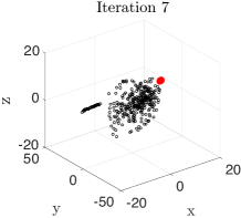
(a)

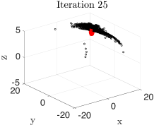
(b)

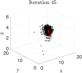
(c)

Figure 4: Evolution of $\mathcal{X}$ over many iterations.

In Fig. 4(a), 4(b), 4(c), the process by which the training set $\mathcal{X}$ iteratively changes from the initial training set $\mathcal{D}_{2}$ to encompassing $\mathcal{X}_{\epsilon}$ is shown. Here, the red states represent the set $\mathcal{X}_{\epsilon}$ and the black states represent the current states in $\mathcal{X}$. In the early iterations (Fig. 4(a)), the NN explores outward from the initial training set, frequently making mistakes, resulting in the states in $\mathcal{X}$ being very far away from $\bar{x}$. As the iteration number increases, the trajectory ambiguous training set $\mathcal{D}_{2}$ is gradually cut down, and eventually the NN begins to predict controls $\hat{u}_{i}(\cdot)$ that drive to states $\hat{x}_{i}$ in an arc that heavily intersects $\mathcal{X}_{\epsilon}$. This can be seen in Fig. 4(b). By the end of the training process, the $\mathcal{R}_{O}$ conical target filter prunes the states outside of the $\mathcal{X}_{\epsilon}$. This can be seen in Fig. 4(c).

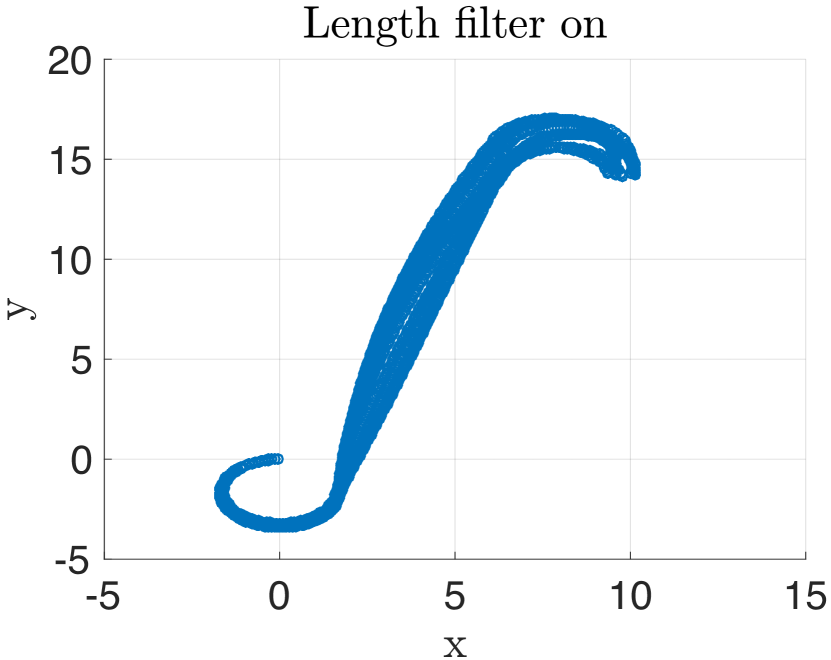
(a)

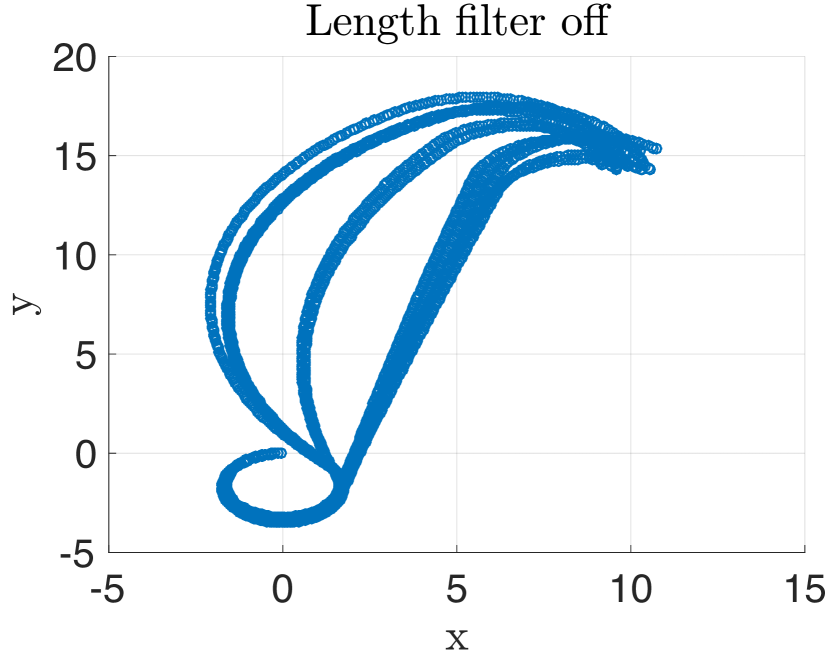
(b)

Figure 5: Effect of the length filter on quality of $\mathcal{X}$. (5(a)) shows $\mathcal{X}$ when the filter is on, and (5(b)) shows $\mathcal{X}$ when it is off.

The length filter also enables our method to be robust to suboptimal training data. If we provide the neural net with a mixture of optimal and suboptimal training data, the length filter improves the quality of $\mathcal{X}$ by removing many states generated by using suboptimal control (Figure 5(a)), compared to without the length filter (Figure 5(b)).

VI-E2 Value Function Comparison

Using level set methods [11], we computed $V(x,t)$, and compared the true value function, $V(\bar{x},t_{0}^{*})$ and the approximate value function, $\hat{V}(\bar{x},\hat{T})$ computed for several states in Table I. $t_{0}^{*}$ denotes the time component of the optimal solution of (3).

State $\bar{x}$	NN Cost $\hat{V}(\bar{x},\hat{T})$	True Cost $V(\bar{x},t_{0}^{*})$
$(-12,5,2)$	$26.51$	$14.84$
$(-10,0,0)$	$10.23$	$10.00$
$(1,1,6)$	$9.93$	$7.40$
$(10,-4,-3)$	$16.20$	$13.36$

TABLE I: Trajectory values (seconds)

VI-E3 Computation Time

Synthesizing control using our NN-based approach allows for large time complexity improvements in comparison to using level set methods. On a 2012 MacBook Pro laptop, data generation requires approximately 3 minutes, and controller synthesis from this data and simulation requires 2 minutes on average. Since the region of the state space we are considering is quite large, and the target set is quite small (a singleton), the level set methods approach is intractable on this laptop, and requires 4 days on a desktop computer with a Core i7-5820K processor and 128 GB of RAM.

There are also large spatial savings by using the NN. For example, $\mathcal{X}$ and $\hat{V}$ for one particular corridor computed between $(10,-1,-3)$ and $(0,0,0)$ requires only 179 MB, while a reachable set computed over that horizon on a very low resolution grid requires approximately 7 GB.

As can be seen from this and the previous sections, using level set methods not only is more time-consuming compared to using our NN-based approach, but also does not guarantee a more shorter trajectory due to discretization error.

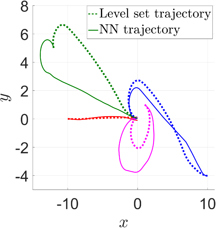
Figure 6: Trajectories generated using level set methods (dashed) and using our NN-based method (solid). Each color corresponds to a different initial state $\bar{x}$.

VII Conclusions and Future Work

Our NN-based grid-free method computes an upper bound of the optimal value function in a region of the state space that contains the initial state, the target set, and a feasible trajectory. By combining the strengths of dynamic programming-based and machine learning-based approaches, we greatly alleviate the curse of dimensionality while maintaining a desired direction of conservatism, effectively avoiding the shortcomings of both types of approaches.

Using a numerical example, we demonstrate that our approach can successfully generate a value function approximation in multiple test cases for the Dubins car. We are even able to approximate value function values in regions that are very far from the target set, a very computationally expensive task for dynamic programming-based approaches. Our approximate value function is able to drive the Dubins car from many different initial conditions to the target set.

Although our current results are promising, much more investigation is still needed to make our approach more practical and applicable to more scenarios. For example, better intuition for the choice of accept regions in the filtering process is needed to extend our approach to other systems. We currently plan to investigate applying our method to the 6D engine-out plane [42] as well as a 12D quadrotor model. In addition to path planning, we also hope to extend our theory to provide safety guarantees and robustness against disturbances. Such extensions are non-trivial due to the different roles that the control and disturbance inputs play in the system dynamics.

References

- [1] Joint Planning and Development Office, “Unmanned Aircraft Systems (UAS) Comprehensive Plan: A Report on the Nation’s UAS Path Forward,” Tech. Rep., 2013. [Online]. Available: http://www.faa.gov/about/...UAS{\_}Comprehensive{\_}Plan.pdf
- [2] K. Fehrenbacher, “Feds Say Safety Is the Key to the Future of Autonomous Cars,” http://fortune.com/2016/07/19/safety-feds-autonomous-cars/.
- [3] Amazon, “Amazon Prime Air,” http://www.amazon.com/b?node=8037720011.
- [4] BBC News, “Google plans drone delivery service for 2017,” http://www.bbc.co.uk/news/technology-34704868, 2015.
- [5] AUVSI News, “UAS Aid in South Carolina Tornado Investigation,” http://www.auvsi.org/blogs/auvsi-news/2016/01/29/tornado, 2016.
- [6] P. Kopardekar, J. Rios, T. Prevot, M. Johnson, J. Jung, and J. E. R. Iii, “Unmanned Aircraft System Traffic Management ( UTM ) Concept of Operations,” 16th AIAA Aviation Technology, Integration, and Operations Conference, pp. 1–16. [Online]. Available: http://arc.aiaa.org/doi/pdf/10.2514/6.2016-3292
- [7] P. Varaiya, “On the existence of solutions to a differential game,” SIAM Journal on Control, vol. 5, no. 1, pp. 153–162, 1967.
- [8] L. C. Evans and P. E. Souganidis, “Differential games and representation formulas for solutions of {Hamilton-Jacobi-Isaacs} equations,” Indiana Univ. Math. J., vol. 33, no. 5, pp. 773–797, 1984.
- [9] E. N. Barron, “Differential games with maximum cost,” Nonlinear Analysis, vol. 14, no. 11, pp. 971–989, jun 1990.
- [10] C. J. Tomlin, J. Lygeros, and S. Sastry, “A Game Theoretic Approach to Controller Design for Hybrid Systems,” Proceedings of IEEE, vol. 88, no. 7, pp. 949–969, jul 2000.
- [11] I. M. Mitchell, A. M. Bayen, and C. J. Tomlin, “A time-dependent Hamilton-Jacobi formulation of reachable sets for continuous dynamic games,” IEEE Transactions on Automatic Control, vol. 50, no. 7, pp. 947–957, 2005.
- [12] K. Margellos and J. Lygeros, “Hamilton-Jacobi Formulation for Reach-Avoid Differential Games,” IEEE Transactions on Automatic Control, vol. 56, no. 8, pp. 1849–1861, aug 2011.
- [13] O. Bokanowski, N. Forcadel, and H. Zidani, “Reachability and Minimal Times for State Constrained Nonlinear Problems without Any Controllability Assumption,” SIAM Journal on Control and Optimization, vol. 48, no. 7, pp. 4292–4316, jan 2010.
- [14] J. F. Fisac, M. Chen, C. J. Tomlin, and S. S. Sastry, “Reach-avoid problems with time-varying dynamics, targets and constraints,” in Proceedings of the 18th International Conference on Hybrid Systems Computation and Control - HSCC ’15. New York, New York, USA: ACM Press, 2015, pp. 11–20.
- [15] J. Ding, J. Sprinkle, S. S. Sastry, and C. J. Tomlin, “Reachability calculations for automated aerial refueling,” in Proceedings of the IEEE Conference on Decision and Control, Cancun, Mexico, 2008, pp. 3706–3712.
- [16] M. Chen, Q. Hu, C. Mackin, J. F. Fisac, and C. J. Tomlin, “Safe platooning of unmanned aerial vehicles via reachability,” in 2015 54th IEEE Conference on Decision and Control (CDC), vol. 2016-Febru. IEEE, dec 2015, pp. 4695–4701.
- [17] A. Majumdar, R. Vasudevan, M. M. Tobenkin, and R. Tedrake, “Convex optimization of nonlinear feedback controllers via occupation measures,” The International Journal of Robotics Research, vol. 33, no. 9, pp. 1209–1230, aug 2014.
- [18] T. Dreossi, T. Dang, and C. Piazza, “Parallelotope Bundles for Polynomial Reachability,” in Proceedings of the 19th International Conference on Hybrid Systems: Computation and Control - HSCC ’16. New York, New York, USA: ACM Press, 2016, pp. 297–306.
- [19] J. Darbon and S. Osher, “Algorithms for overcoming the curse of dimensionality for certain Hamilton–Jacobi equations arising in control theory and elsewhere,” Research in the Mathematical Sciences, vol. 3, no. 1, p. 19, dec 2016.
- [20] I. M. Mitchell and C. J. Tomlin, “Overapproximating Reachable Sets by Hamilton-Jacobi Projections,” Journal of Scientific Computing, vol. 19, no. 1-3, pp. 323–346, 2003.
- [21] J. McGrew, L. Bush, J. How, N. Roy, and B. Williams, “Air Combat Strategy Using Approximate Dynamic Programming,” AIAA Guidance, Navigation and Control Conference and Exhibit, pp. 1–33, aug 2008.
- [22] M. Chen*, S. Herbert*, and C. J. Tomlin, “Fast Reachable Set Approximations via State Decoupling Disturbances,” in 55th IEEE Conference on Decision and Control (to appear), 2016.
- [23] G. Frehse, C. Le Guernic, A. Donzé, S. Cotton, R. Ray, O. Lebeltel, R. Ripado, A. Girard, T. Dang, and O. Maler, “Spaceex: Scalable verification of hybrid systems,” in Proc. 23rd International Conference on Computer Aided Verification (CAV), ser. LNCS, S. Q. Ganesh Gopalakrishnan, Ed. Springer, 2011.
- [24] P. S. Duggirala, M. Potok, S. Mitra, and M. Viswanathan, “C2e2: A tool for verifying annotated hybrid systems,” in Proceedings of the 18th International Conference on Hybrid Systems: Computation and Control, ser. HSCC ’15. New York, NY, USA: ACM, 2015, pp. 307–308.
- [25] X. Chen, E. Ábrahám, and S. Sankaranarayanan, “Flow*: An analyzer for non-linear hybrid systems,” in Computer Aided Verification - 25th International Conference, CAV 2013, Saint Petersburg, Russia, July 13-19, 2013. Proceedings, 2013, pp. 258–263.
- [26] S. Kong, S. Gao, W. Chen, and E. M. Clarke, “dreach: -reachability analysis for hybrid systems,” in Tools and Algorithms for the Construction and Analysis of Systems - 21st International Conference, TACAS 2015, Held as Part of the European Joint Conferences on Theory and Practice of Software, ETAPS 2015, London, UK, April 11-18, 2015. Proceedings, 2015, pp. 200–205.
- [27] L. Grne and J. Pannek, Nonlinear Model Predictive Control: Theory and Algorithms. Springer Publishing Company, Incorporated, 2013.
- [28] I. M. I. M. Gelʹfand, R. A. Silverman, and S. V. S. V. Fomin, Calculus of variations, rev. english ed. / translated and edited by richard a. silverman ed. Englewood Cliffs, N.J. : Prentice-Hall, 1963.
- [29] M. S. Aronna, J. F. Bonnans, and P. Martinon, “A shooting algorithm for optimal control problems with singular arcs,” J. Optimization Theory and Applications, vol. 158, no. 2, pp. 419–459, 2013.
- [30] Y. Becerikli, A. F. Konar, and T. Samad, “Intelligent optimal control with dynamic neural networks.” Neural networks : the official journal of the International Neural Network Society, vol. 16, no. 2, pp. 251–9, mar 2003.
- [31] B. S. Kim and A. J. Calise, “Nonlinear Flight Control Using Neural Networks,” Journal of Guidance, Control, and Dynamics, vol. 20, no. 1, pp. 26–33, jan 1997.
- [32] R. E. Allen, A. A. Clark, J. A. Starek, and M. Pavone, “A Machine Learning Approach for Real-Time Reachability Analysis Ross,” in International Conference on Intelligent Robots and Systems, no. Iros. IEEE, sep 2014, pp. 2202–2208.
- [33] B. Djeridane and J. Lygeros, “Neural approximation of PDE solutions: An application to reachability computations,” in Proceedings of the 45th IEEE Conference on Decision and Control. IEEE, 2006, pp. 3034–3039.
- [34] K. N. Niarchos and J. Lygeros, “A Neural Approximation to Continuous Time Reachability Computations,” in Proceedings of the 45th IEEE Conference on Decision and Control. IEEE, 2006, pp. 6313–6318.
- [35] E. N. Barron and H. Ishii, “The Bellman equation for minimizing the maximum cost,” Nonlinear Analysis, vol. 13, no. 9, pp. 1067–1090, 1989.
- [36] I. Yang, S. Becker-Weimann, M. J. Bissell, and C. J. Tomlin, “One-shot computation of reachable sets for differential games,” in Proceedings of the 16th international conference on Hybrid systems: computation and control - HSCC ’13. New York, New York, USA: ACM Press, 2013, p. 183.
- [37] J. A. Sethian, “A fast marching level set method for monotonically advancing fronts,” Pnas, vol. 93, no. 4, pp. 1591–1595, 1996.
- [38] S. Osher and R. Fedkiw, Level Set Methods and Dynamic Implicit Surfaces. Springer-Verlag, 2006.
- [39] I. Mitchell, “A toolbox of level set methods,” Tech. Rep., 2007.
- [40] G. Cybenko, “Approximation by Superposition of a Sigmoidal Function.”
- [41] L. E. Dubins, “On Curves of Minimal Length with a Constraint on Average Curvature, and with Prescribed Initial and Terminal Positions and Tangents,” American Journal of Mathematics, vol. 79, no. 3, pp. 497–516, jul 1957.
- [42] A. Adler, A. Bar-Gill, and N. Shimkin, “Optimal flight paths for engine-out emergency landing,” in Proceedings of the 2012 24th Chinese Control and Decision Conference, CCDC 2012. IEEE, may 2012, pp. 2908–2915.