The Control of the False Discovery Rate in Fixed Sequence Multiple Testing

Abstract

Controlling the false discovery rate (FDR) is a powerful approach to multiple testing. In many applications, the tested hypotheses have an inherent hierarchical structure. In this paper, we focus on the fixed sequence structure where the testing order of the hypotheses has been strictly specified in advance. We are motivated to study such a structure, since it is the most basic of hierarchical structures, yet it is often seen in real applications such as statistical process control and streaming data analysis. We first consider a conventional fixed sequence method that stops testing once an acceptance occurs, and develop such a method controlling the FDR under both arbitrary and negative dependencies. The method under arbitrary dependency is shown to be unimprovable without losing control of the FDR and unlike existing FDR methods; it cannot be improved even by restricting to the usual positive regression dependence on subset (PRDS) condition. To account for any potential mistakes in the ordering of the tests, we extend the conventional fixed sequence method to one that allows more but a given number of acceptances. Simulation studies show that the proposed procedures can be powerful alternatives to existing FDR controlling procedures. The proposed procedures are illustrated through a real data set from a microarray experiment.

AMS 2000 subject classifications: Primary 62J15

KEY WORDS: Arbitrary dependence, false discovery rate, fixed sequence, multiple testing, negative association, PRDS property, $p$-values.

1 Introduction

In many applications of multiple testing, such as genomic research, clinical trials, and statistical process control, the hypotheses are so structured that they are to be tested in a particular sequence. This structure may be a natural one, as in Goeman and Mansmann (2008), where Gene Ontology imposes a directed acyclic graph structure onto the tested hypotheses, or can be formed by using a data-driven approach for specifying the testing order of the hypotheses, as in Kropf and L$\ddot{a}$uter (2002), Kropf et al. (2004), Westfall et al. (2004), Hommel and Kropf (2005), Finos and Farcomeni (2011), etc. In some applications, it is not even possible to use the conventional $p$-value based multiple testing methods, because of some inherent structure among the tested hypotheses. For example, the hypotheses associated with stream data in sequential change detection problems (Ross et al., 2011) have a natural temporal structure, but none of conventional methods, such as the stepwise procedures, which are applicable only when all of $p$-values are available, can be used here since the decision concerning a hypothesis has to be made even before the data associated with the remaining hypotheses are observed.

Some progress has been made in testing structured hypotheses. However, it has been primarily focused on controlling the familywise error rate (FWER) (Maurer et al., 1995; Westfall and Krishen, 2001; Wiens, 2003; Wiens and Dmitrienko, 2005; Hommel et al., 2007; Huque and Alosh, 2008; Li and Mehrotra, 2008; Rosenbaum, 2008; Wiens and Dmitrienko, 2010; Millen and Dmitrienko, 2011; Dmitrienko et al., 2013). There are few results towards controlling the false discovery rate (FDR) while accounting for the structure of the tested hypotheses. Benjamini and Heller (2007), Heller et al. (2009), and Mehrotra and Heyse (2004) developed methods for testing hypotheses with a specific hierarchical structure where the structure is limited to only two levels. Yekutieli (2008) discussed a method that controls the FDR when the tested hypotheses have a general hierarchical structure. However, that method is shown to control the FDR only under independence.

The primary objective of this paper is to help advance the theory and methods on controlling the FDR for testing structured hypotheses. We do so by focusing on a structure where the hypotheses have a fixed pre-defined testing order since this is the simplest of hierarchical structures, yet it is often seen in real applications such as clinical trials, statistical process control and streaming data analysis. For such a structure, we will refer to it as a fixed sequence structure throughout this paper. Very recently, several methods have been introduced for controlling FDR while testing pre-ordered hypotheses. Farcomeni and Finos (2013) developed a ‘single-step’ FDR controlling method for testing hypotheses with the same critical value $\alpha$, which tests each hypothesis at level $\alpha$ until a stopping condition is reached. Barber and Candes (2015), G’Sell et al. (2016) and Li and Barber (2016) developed several different ‘step-up’ FDR controlling procedures in the context of high-dimensional regression for testing hypotheses with fixed sequence structure for which hypotheses are tested from highest-ranked to lowest-ranked, and Lei and Withian (2016) performed asymptotic power analysis for such ‘step-up’ procedures. In addition, Javanmard and Montanari (2015) developed procedures for controlling the FDR in an online manner while testing a sequence of possibly infinite pre-ordered hypotheses.

In this paper, we develop ‘step-down’ FDR controlling methods that fully exploit the fixed sequence structural information, in which hypotheses are tested from lowest-ranked to highest-ranked. We first consider a conventional fixed sequence multiple testing method that keeps rejecting until an acceptance occurs and develop such a method controlling the FDR under arbitrary dependence. It is shown to be optimal in the sense that it cannot be improved by increasing even one of its critical values without losing control over the FDR, or even by imposing a positive dependence condition on the $p$-values, such as the standard PRDS (positive regression dependence on subset) condition of Benjamini and Yekutieli (2001). This is different from what happens in case of non-fixed sequence multiple testing. For instance, the so-called BY method of Benjamini and Yekutieli (2001) that controls the FDR under arbitrary dependence can be improved significantly by the BH method of Benjamini and Hochberg (1995) by imposing this PRDS condition. Since our procedure cannot be improved under positive dependence, we consider the case of negative dependence and develop a more powerful conventional fixed sequence multiple testing method controlling the FDR under negative dependence which includes independence as a special case.

There is a potential for loss of power in a conventional fixed sequence multiple testing method if the ordering of the hypotheses, particularly for the earlier ones, does not match with that of their true effect sizes, potentially leading to some earlier hypothesis being accepted and the follow-up hypotheses having no chance to be tested. To mitigate that, we consider generalizing the conventional fixed sequence multiple testing to one that allows more than one but a pre-specified number of acceptances, and develop such generalized fixed sequence multiple testing methods controlling the FDR under both arbitrary dependence and independence.

It is not always the case in real data applications that the hypotheses will have a natural fixed sequence structure or information about how to order them will be available a priori. Nevertheless, the data itself can often provide information on how to order the hypotheses. In this paper, we discuss such a data-driven ordering strategy which can be applied to a broad spectrum of multiple testing problems such as one-sample and two-sample t-tests, and one-sample and two-sample nonparametric tests. Through simulation studies and a real microarray data analysis, this strategy coupled with our proposed fixed sequence methods is seen to perform favorably against the corresponding non-fixed sequence methods under certain settings.

The paper is organized as follows. With some concepts and background information given in Section 2, we present the developments of our conventional and generalized fixed sequence procedures controlling the FDR under various dependencies in Sections 3 and 4, respectively. Our fixed sequence procedures coupled with a data-driven ordering strategy for the hypotheses are applied to a real microarray data in Section 5. The findings from some simulation studies on the performances of our procedures are given in Section 6. Some concluding remarks are made in Section 7 and proofs of some results are given in the Appendix.

2 Preliminaries

Suppose that $H_{i},i=1,\ldots,m$, are the $m$ null hypotheses that are ordered a priori and are to be simultaneously tested based on their respective $p$-values $P_{i},i=1,\ldots,m$. Let $m_{0}$ and $m_{1}$ of these null hypotheses be true and false, respectively. For notational convenience, we denote the index of the $i$th true null hypothesis by $u_{i}$ and the set of indices of the true null hypotheses by $I_{0}$. Let $V$ and $S$ be the numbers of true and false null hypotheses, respectively, among the $R$ rejected null hypotheses in a multiple testing procedure. Then, the familywise error rate (FWER) and false discovery rate (FDR) of this procedure are defined respectively as $\text{FWER}=\text{Pr}(V>0)$ and $\text{FDR}=E\left(\frac{V}{\max(R,1)}\right)=E\left(\frac{V}{V+S}1_{\{V>0\}}\right)$.

Typically, the hypotheses are ordered based on their $p$-values and multiple testing is carried out using a stepwise or single-step procedure. However, when these hypotheses are ordered a prior and not according to their $p$-values, multiple testing is often performed using a fixed sequence method. Given a non-decreasing sequence of critical constants $0<\alpha_{1}\leq\ldots\leq\alpha_{m}$, a conventional fixed sequence method is defined as follows:

Definition 1

(Conventional fixed sequence method)

1. If $P_{1}\leq\alpha_{1}$, then reject $H_{1}$ and continue to test $H_{2}$; otherwise, stop.

2. If $P_{i}\leq\alpha_{i}$ then reject $H_{i}$ and continue to test $H_{i+1}$; otherwise, stop.

Thus, a conventional fixed sequence method continues testing in the pre-determined order as long as rejections occur. Once an acceptance occurs, it stops testing the remaining hypotheses. In Section 4, we will generalize a conventional fixed sequence method to allow a given number of acceptances. It should be noted that a conventional fixed sequence method with common critical constant $\alpha$, which is often called the fixed sequence procedure in the literature, strongly controls the FWER at level $\alpha$ (Maurer et al., 1995). We will refer to it as the FWER fixed sequence procedure in this paper in order to distinguish it from other fixed sequence methods designed to control the FDR.

Regarding assumptions we make about the $p$-values in this paper, we assume that the true null $p$-values, which we denote for notational convenience by $\widehat{P}_{i}$, for $i=1,\ldots,m_{0}$, are marginally distributed as follows:

$$\mathrm{Pr}\left(\widehat{P}_{i}\leq p\right)\leq p\text{~{}~{}~{}for~{}any~{}}p\in(0,1).$$ (1)

One of several types of dependence, like arbitrary dependence, positive dependence, negative dependence, and independence, has been assumed to characterize a dependence structure among the $p$-values.

By arbitrary dependence, we mean that the $p$-values do not have any specific form of dependence. The positive dependence is characterized by the positive regression dependence on subset (PRDS) property (Benjamini and Yekutieli, 2001) as defined below:

Definition 2

(PRDS) The vector of $p$-values $\vec{P}$ is PRDS on the vector of null $p$-values $\vec{P_{0}}=(\widehat{P}_{1},\ldots,\widehat{P}_{m_{0}})$ if for every increasing set $D$ and for each $i=1,\ldots,m_{0}$, the conditional probability $\mathrm{Pr}\left(\vec{P}\in D\;\middle|\;\widehat{P}_{i}=p\right)$ is non-decreasing in $p$.

Several multivariate distributions possess this property (see, for instance, Benjamini and Yekutieli, 2001; Sarkar, 2002). The negative dependence is characterized by the following property:

Definition 3

(Negative Association) The vector of $p$-values $\vec{P}$ is negatively associated with null $p$-values if for each $i=1,\ldots,m_{0}$, the following inequality holds:

$$~{}~{}\mathrm{Pr}\left(\widehat{P}_{i}\leq p_{u_{i}},P_{j}\leq p_{j},j=1,\ldots,m,\text{~{}with~{}}j\neq u_{i}\right)$$ (2)

$$\leq \mathrm{Pr}\left(\widehat{P}_{i}\leq p_{u_{i}}\right)\mathrm{Pr}\left(P_{j}\leq p_{j},j=1,\ldots,m,\text{~{}with~{}}j\neq u_{i}\right),$$

for all fixed $p_{j}$’s.

Several multivariate distributions posses the conventional negative association property, including multivariate normal with non-positive correlation, multinomial, dirichlet, and multivariate hypergeometric (Joag Dev and Proschan, 1983). It is easily seen that independence is a special case of negative dependence.

3 Conventional Fixed Sequence Procedures

In this section, we present the developments of two simple conventional fixed sequence procedures controlling the FDR under both arbitrary dependence and negative dependence conditions on the $p$-values.

3.1 Procedure under arbitrary dependence

Since the FDR is more liberal than the FWER, a conventional fixed sequence method controlling the FDR under arbitrary dependence is expected to have critical values that are at least as large as $\alpha$, the common critical constant for the FWER fixed sequence method. In the following, we present such a simple conventional fixed sequence FDR controlling procedure.

Theorem 3.1

Consider a conventional fixed sequence procedure with critical constants

$$\alpha^{(1)}_{i}=\min\left(\frac{m\alpha}{m-i+1},1\right),\;i=1,\dots,m.$$

• This procedure strongly controls the FDR at level $\alpha$ under arbitrary dependence of the $p$-values.

• One cannot increase even one of the critical constants $\alpha^{(1)}_{i},i=1,\dots,m,$ while keeping the remaining fixed without losing control of the FDR. This is true even when $\vec{P}$ is assumed to be PRDS on $\vec{P}_{0}$.

Proof of (i). Since $u_{1}$ is the index of the first true null hypothesis, the first $u_{1}-1$ null hypotheses are all false. Note that the event $\{V>0\}$ implies that $S\geq u_{1}-1$ and $\hat{P}_{1}\leq\alpha^{(1)}_{u_{1}}$, and therefore we have

FDR $$=E\left(\frac{V}{V+S}1_{\{V>0\}}\right)\leq E\left(\frac{m_{0}}{m_{0}+u_{1}-1}1_{\{V>0\}}\right)$$

$$=\frac{m_{0}}{m_{0}+u_{1}-1}Pr(V>0)\leq\frac{m_{0}}{m_{0}+u_{1}-1}Pr(\hat{P}_{1}\leq\alpha^{(1)}_{u_{1}})$$

$$\leq\frac{m-u_{1}+1}{m}\alpha^{(1)}_{u_{1}}\leq\alpha.$$

The first inequality follows from the fact that $V/(V+S)$ is an increasing function of $V$ and a decreasing function of $S$. The third inequality follows from the fact that $m_{0}/(m_{0}+u_{1}-1)$ is an increasing function of $m_{0}$ and $m_{0}\leq m-u_{1}+1$ since there are at least $u_{1}-1$ false nulls. This proves part (i).

For a proof of part (ii), see Appendix.  

Remark 3.1

Theorem 3.1 shows that when controlling the FDR under arbitrary dependence, the operating characteristic of the proposed fixed sequence method is much different from that of the usual stepwise procedure of Benjamini and Yekutieli (Benjamini and Yekutieli, 2001) that relys on $p$-value based ordering of the hypotheses. It cannot be further improved, even by imposing the PRDS assumption on the $p$-values, unlike the BY procedure that is known to be greatly improved by the Benjamini-Hochberg (BH) procedure under such positive dependence. Also, as shown in our proof of Theorem 3.1(ii) under arbitrary dependence (see Appendix), the least favorable configuration (the configuration which leads to the largest error rate, see Finner and Roters, 2001) of the newly suggested fixed sequence FDR controlling procedure is when the ordering of the hypotheses is perfect (i.e, when all the false null hypotheses are tested before the true ones), the false null $p$-values are all $0$ with probability 1, and the true null $p$-values are the same with each following $U(0,1)$ distribution. This least favorable configuration is much different from that given in Guo and Rao (2008) for the BY procedure under arbitrary dependence.

Although the procedure in Theorem 3.1 cannot be improved under the PRDS condition, we consider in the next subsection the condition of negative dependence which includes independence as a special case, and under such condition, develop a more powerful conventional fixed sequence method that controls the FDR.

3.2 Procedure under negative dependence

When the $p$-values are negatively associated as defined in Section 2, the critical constants of the conventional fixed sequence procedure in Theorem 3.1 can be further improved as in the following:

Theorem 3.2

The conventional fixed sequence method with critical constants

$$\alpha^{(2)}_{i}=\frac{i\alpha}{1+(i-1)\alpha},i=1,\ldots,m$$

strongly controls the FDR at level $\alpha$ when the $p$-values are negatively associated on the true null $p$-values.

To prove Theorem 3.2, we use the following lemma, with proof given in Appendix:

Lemma 3.1

Let $m_{0,i}$ and $m_{1,i}$ respectively denote the numbers of true and false null hypotheses among the first $i$ null hypotheses, and

$$d_{i}=\begin{cases}1_{\{i\in I_{0}\}}&\text{ if }~{}i=1\\ (m_{1,i-1}1_{\{i\in I_{0}\}}-m_{0,i-1}1_{\{i\notin I_{0}\}})/(i(i-1))&\text{ if }~{}i>1.\\ \end{cases}$$

Then, the FDR of any fixed sequence procedure can be expressed as

$$\emph{FDR}=\displaystyle\sum\limits_{\begin{subarray}{c}i=1\end{subarray}}^{\begin{subarray}{c}m\end{subarray}}d_{i}\mathrm{Pr}\left(R\geq i\right).$$

Proof of Theorem 3.2. If $u_{1}=1$, then

$$\text{FDR}\leq\text{FWER}=\mathrm{Pr}\left(V>0\right)=\mathrm{Pr}\left(\widehat{P}_{1}\leq\alpha^{(2)}_{1}\right)\leq\alpha.$$

If $u_{1}>1$, then by Lemma 3.1,

FDR $$=\displaystyle\sum\limits_{\begin{subarray}{c}i=1\end{subarray}}^{\begin{subarray}{c}m\end{subarray}}d_{i}\mathrm{Pr}\left(R\geq i\right)=\displaystyle\sum\limits_{\begin{subarray}{c}i=u_{1}\end{subarray}}^{\begin{subarray}{c}m\end{subarray}}d_{i}\mathrm{Pr}\left(R\geq i\right)$$

$$=\displaystyle\sum\limits_{\begin{subarray}{c}i=u_{1}\end{subarray}}^{\begin{subarray}{c}m\end{subarray}}\left(d_{i}+\frac{m_{1,i}\alpha}{i}\right)\mathrm{Pr}\left(R\geq i\right)-\displaystyle\sum\limits_{\begin{subarray}{c}i=u_{1}\end{subarray}}^{\begin{subarray}{c}m\end{subarray}}\frac{m_{1,i}\alpha}{i}\mathrm{Pr}\left(R\geq i\right).$$ (3)

The second equality follows from the fact that $d_{i}=0$ for $i=1,\dots,u_{1}-1$.

For each $i=u_{1},\dots,m$, the following inequality holds.

$$\left(d_{i}+\frac{m_{1,i}\alpha}{i}\right)\mathrm{Pr}\left(R\geq i\right)\leq\frac{m_{1,i-1}\alpha}{i-1}Pr(R\geq i-1).$$ (4)

To see this, we consider, separately, the case when $i\in I_{0}$ and when $i\notin I_{0}$. Suppose $i\in I_{0}$, then $m_{1,i-1}=m_{1,i}$ and

$$\left(d_{i}+\frac{m_{1,i}\alpha}{i}\right)\mathrm{Pr}\left(R\geq i\right)$$

$$= \left(\frac{m_{1,i-1}}{i(i-1)}+\frac{m_{1,i-1}\alpha}{i}\right)\mathrm{Pr}\left(P_{1}\leq\alpha^{(2)}_{1},\ldots,P_{i-1}\leq\alpha^{(2)}_{i-1},P_{i}\leq\alpha^{(2)}_{i}\right)$$

$$\leq \frac{m_{1,i-1}\left(1+(i-1)\alpha\right)}{i(i-1)}\mathrm{Pr}\left(P_{1}\leq\alpha^{(2)}_{1},\ldots,P_{i-1}\leq\alpha^{(2)}_{i-1}\right)\mathrm{Pr}\left(P_{i}\leq\alpha^{(2)}_{i}\right)$$

$$\leq \frac{m_{1,i-1}\alpha}{i-1}Pr(R\geq i-1).$$

The first and second inequalities follow from (2) and (1), respectively.

Now suppose $i\notin I_{0}$, then $m_{1,i}=m_{1,i-1}+1$ and

$$\left(d_{i}+\frac{m_{1,i}\alpha}{i}\right)\mathrm{Pr}\left(R\geq i\right)=\left(-\frac{m_{0,i-1}}{i(i-1)}+\frac{(m_{1,i-1}+1)\alpha}{i}\right)\mathrm{Pr}\left(R\geq i\right)$$

$$\leq \left(-\frac{m_{0,i-1}\alpha}{i(i-1)}+\frac{(m_{1,i-1}+1)\alpha}{i}\right)\mathrm{Pr}\left(R\geq i\right)$$

$$= \frac{m_{1,i-1}\alpha}{i-1}\mathrm{Pr}\left(R\geq i\right)\leq\frac{m_{1,i-1}\alpha}{i-1}\mathrm{Pr}\left(R\geq i-1\right).$$

In the second equality, we use the fact that $m_{0,i-1}+m_{1,i-1}=i-1$.

Applying (4) to (3), we have

FDR $$= \displaystyle\sum\limits_{\begin{subarray}{c}i=u_{1}\end{subarray}}^{\begin{subarray}{c}m\end{subarray}}\left(d_{i}+\frac{m_{1,i}\alpha}{i}\right)\mathrm{Pr}\left(R\geq i\right)-\displaystyle\sum\limits_{\begin{subarray}{c}i=u_{1}\end{subarray}}^{\begin{subarray}{c}m\end{subarray}}\frac{m_{1,i}\alpha}{i}\mathrm{Pr}\left(R\geq i\right)$$

$$\leq \displaystyle\sum\limits_{\begin{subarray}{c}i=u_{1}\end{subarray}}^{\begin{subarray}{c}m\end{subarray}}\frac{m_{1,i-1}\alpha}{i-1}\mathrm{Pr}\left(R\geq i-1\right)-\displaystyle\sum\limits_{\begin{subarray}{c}i=u_{1}\end{subarray}}^{\begin{subarray}{c}m\end{subarray}}\frac{m_{1,i}\alpha}{i}\mathrm{Pr}\left(R\geq i\right)$$

$$= \alpha\mathrm{Pr}\left(R\geq u_{1}-1\right)-\frac{m_{1}\alpha}{m}\mathrm{Pr}\left(R=m\right)$$

$$\leq\alpha.$$

The equality follows from that fact that $m_{1,u_{1}-1}=u_{1}-1$, since the first $u_{1}-1$ hypotheses are false.  

Remark 3.2

The conventional fixed sequence procedure in Theorem 3.2 is nearly optimal in the sense that the upper bound of the FDR of this procedure is very close to $\alpha$ under certain configurations. Consider the following configuration: All the false null hypotheses are tested before the true null hypotheses, the false null $p$-values are all $0$ with probability 1, and the true null $p$-values are independently distributed as $U(0,1)$. Under this configuration, it is easy to check that (4) becomes an equality. Following the proof of Theorem 3.2, the FDR of this procedure is exactly $\alpha-\frac{m_{1}\alpha}{m}\mathrm{Pr}\left(R=m\right)$. When $m_{1}/m$ approaches to $\pi_{1}$ as $m\rightarrow\infty$ with $0\leq\pi_{1}<1$, an approximate lower bound of the FDR is $\alpha-\pi_{1}\alpha e^{-(1-\pi_{1})\frac{1-\alpha}{\alpha}}$.

To see why, we first note that

$$\frac{m_{1}\alpha}{m}\mathrm{Pr}\left(R=m\right)=\frac{m_{1}\alpha}{m}\displaystyle\prod\limits_{i=m_{1}+1}^{m}\alpha^{(2)}_{i}<\frac{m_{1}\alpha}{m}(\alpha^{(2)}_{m})^{m-m_{1}}.$$

Then, by simple calculation, we have

$$\lim_{m\rightarrow\infty}\text{FDR}\geq\alpha-\lim_{m\rightarrow\infty}\frac{m_{1}\alpha}{m}(\alpha^{(2)}_{m})^{m-m_{1}}$$

$$= \alpha-\lim_{m\rightarrow\infty}\frac{m_{1}\alpha}{m}\left(1+\frac{1-\alpha}{\alpha}\frac{1}{m}\right)^{-m(1-\frac{m_{1}}{m})}$$

$$= \alpha-\pi_{1}\alpha e^{-(1-\pi_{1})\frac{1-\alpha}{\alpha}}.$$

This lower bound of the FDR is very close to the pre-specified level $\alpha$. For example, for large $m$, if $m_{1}/m=0.2$, then with $\alpha=0.05$, the lower bound under the above configuration is about 0.04999975.

Remark 3.3

Figure 1 compares the critical constants for the proposed procedures along with the FWER fixed sequence procedure at level $\alpha$. It should be noted that the first few critical constants are the most important ones. If the first few values are too small, then the procedure might stop too early and the remaining hypotheses will not have a chance to be tested. With this in mind, it can be seen that the critical constants of the procedure introduced in Theorem 3.2 are by far the best, and the critical constants of the procedure in Theorem 3.1 are slightly better than those of the conventional fixed sequence procedure.

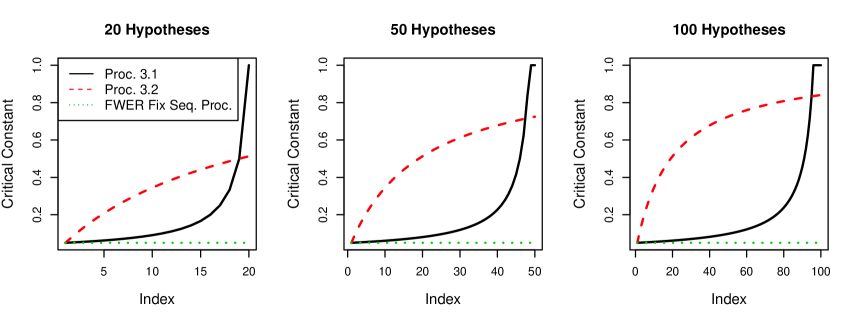
Figure 1: A plot of the critical constants of the procedures in Theorems 3.1 (solid line), 3.2 (dashed line), and the FWER fixed sequence procedure (dotted line) for $m=$20, 50, and 100.

4 Fixed Sequence Procedures that Allow More Acceptances

A conventional fixed sequence method might potentially lose power if an early null hypothesis fails to be rejected, with the remaining hypotheses having no chance of being tested. To remedy this, we generalize a conventional fixed sequence method to one that allows a certain number of acceptances. The procedure will keep testing hypotheses until a pre-specified number of acceptance has been reached. The same idea has also been used by Hommel and Kropf (2005) to develop FWER controlling procedures in fixed-sequence multiple testing.

Suppose $k$ is a pre-specified positive integer and $\alpha_{1}\leq\cdots\leq\alpha_{m}$ is a non-decreasing sequence of critical constants. A fixed sequence method that allows more acceptances is defined below.

Definition 4

(Fixed sequence method stopping on the $k^{th}$ acceptance)

1. If $P_{1}\leq\alpha_{1}$, then reject $H_{1}$; otherwise, accept $H_{1}$. If $k>1$ or $H_{1}$ is rejected, then continue to test $H_{2}$; otherwise stop.

2. If $P_{i}\leq\alpha_{i}$, then reject $H_{i}$; otherwise, accept $H_{i}$. If the number of accepted hypotheses so far is less than $k$, then continue to test $H_{i+1}$; otherwise stop.

It is easy to see that when $k=1$, the fixed sequence method stopping on the $k^{th}$ acceptance reduces to the conventional one.

Theorem 4.1

The fixed sequence method stopping on the $k^{th}$ acceptance with critical constants

$$\alpha^{(3)}_{i}=\begin{cases}\frac{\alpha}{k}&\text{ if }\quad i=1,\dots,k\\ \frac{(m-k+1)\alpha}{(m-i+1)k}&\text{ if }\quad i=k+1,\dots,m\end{cases}$$

strongly controls the FDR at level $\alpha$ under arbitrary dependence of the $p$-values.

Proof. Let $U$ be the index of the first rejected true null hypothesis. If no true null hypotheses are rejected, then set $U=0$. We will show that for $i=1,\ldots,m_{0}$,

$$E\left(\frac{V}{V+S}1_{\{U=u_{i}\}}\right)\leq\frac{\alpha}{k}.$$ (5)

If $i\leq k$, then

$$E\left(\frac{V}{V+S}1_{\{U=u_{i}\}}\right)\leq\mathrm{Pr}\left(U=u_{i}\right)\leq\mathrm{Pr}\left(\hat{P}_{i}\leq\frac{\alpha}{k}\right)\leq\frac{\alpha}{k}.$$

Now, assume $i>k$. Note that the event $\{U=u_{i}\}$ implies $V\leq m-u_{i}+1$ and $S\geq u_{i}-k$, because the first $u_{i}-1$ hypotheses were either false nulls or not rejected true nulls and among the first $u_{i}-1$ hypotheses tested, there can be at most $k-1$ acceptances. Thus,

$$E\left(\frac{V}{V+S}1_{\{U=u_{i}\}}\right)\leq E\left(\frac{m-u_{i}+1}{(m-u_{i}+1)+(u_{i}-k)}1_{\{U=u_{i}\}}\right)$$

$$\leq \frac{m-u_{i}+1}{m-k+1}\mathrm{Pr}\left(\hat{P}_{i}\leq\alpha^{(3)}_{u_{i}}\right)\leq\frac{\alpha}{k}.$$

The first inequality follows from the fact that $V/(V+S)$ is an increasing function of $V$ and a decreasing function of $S$.

From (5), we have

$$\text{FDR}=\displaystyle\sum\limits_{\begin{subarray}{c}i=1\end{subarray}}^{\begin{subarray}{c}\min(m_{0},k)\end{subarray}}E\left(\frac{V}{S+V}1_{\{U=u_{i}\}}\right)\leq\displaystyle\sum\limits_{\begin{subarray}{c}i=1\end{subarray}}^{\begin{subarray}{c}k\end{subarray}}\frac{\alpha}{k}=\alpha,$$

where the first equality follows from the fact that if none of the first $k$ true null hypotheses are rejected, then $V=0$.   

We should point out that the result in Theorem 4.1 is weaker than that in Theorem 3.1, although the method in Theorem 4.1 reduces to that in Theorem 3.1 when $k=1$. More specifically, we cannot prove that the procedure in Theorem 4.1 is optimal in the sense that its critical constants cannot be further improved without losing control of the FDR under arbitrary dependence of the $p$-values. However, under certain distributional assumptions on the $p$-values, the critical constants of this procedure can potentially be improved. In particular, we have the following result.

Theorem 4.2

Consider a fixed sequence method stopping on the $k^{th}$ acceptance with critical constants

$$\alpha^{(4)}_{i}=\frac{(r_{i-1}+1)\alpha}{k+(i-k)\alpha},i=1,\dots,m,$$

where $r_{i}$ is the number of rejections among the first $i$ tested hypotheses, with $r_{0}=0$, for $i=1,\ldots,m$. This procedure strongly controls the FDR at level $\alpha$ if the true null $p$-values are mutually independent and are independent of the false null $p$-values.

Before presenting a proof of the above theorem, let us introduce a few more notations. For $i=1,\ldots,m$, let $V_{i}$ and $S_{i}$ be the numbers of false rejections and true rejections among the first $i$ rejections and $J_{i}$ be the index of the $i^{th}$ rejected hypothesis. If there are less than $i$ rejections, we define $V_{i}=V_{i-1}$, $S_{i}=S_{i-1}$ and $J_{i}=m+1$. In addition, for notational convenience, define $V_{0}=S_{0}=J_{0}=0,V_{0}/0=0,$ and $S_{0}/0=1$.

We use the following two lemmas, with proofs given in Appendix, to prove the theorem.

Lemma 4.1

The FDR of any fixed sequence method stopping on the $k^{th}$ acceptance can be expressed as

$$\emph{FDR}=E\left(\displaystyle\sum\limits_{\begin{subarray}{c}i=1\end{subarray}}^{\begin{subarray}{c}m\end{subarray}}\left(\frac{V_{i}}{i}-\frac{V_{i-1}}{i-1}\right)1_{\{J_{i}<m+1\}}\right).$$

Lemma 4.2

Consider the procedure defined in Theorem 4.2, the following inequality holds for $i=1,\dots,m$,

$$E\left(\left(\frac{V_{i}}{i}-\frac{V_{i-1}}{i-1}\right)1_{\{J_{i}<m+1\}}\right)$$

$$\leq E\left(\frac{(k-J_{i-1}+i-1)\alpha}{k}\frac{S_{i-1}}{i-1}1_{\{J_{i-1}<m+1\}}-\frac{(k-J_{i}+i)\alpha}{k}\frac{S_{i}}{i}1_{\{J_{i}<m+1\}}\right).$$

Proof of Theorem 4.2. By Lemmas 4.1 and 4.2, we have

FDR $$= E\left(\displaystyle\sum\limits_{\begin{subarray}{c}i=1\end{subarray}}^{\begin{subarray}{c}m\end{subarray}}\left(\frac{V_{i}}{i}-\frac{V_{i-1}}{i-1}\right)1_{\{J_{i}<m+1\}}\right)$$

$$\leq E\left(\alpha-\frac{(k-J_{1}+1)\alpha}{k}S_{1}1_{\{J_{i}<m+1\}}\right)$$

$$+~{}E\left(\displaystyle\sum\limits_{\begin{subarray}{c}i=2\end{subarray}}^{\begin{subarray}{c}m\end{subarray}}\left(\frac{(k-J_{i-1}+i-1)\alpha}{k}\frac{S_{i-1}}{i-1}1_{\{J_{i-1}<m+1\}}\right.\right.$$

$$\left.\left.-~{}\frac{(k-J_{i}+i)\alpha}{k}\frac{S_{i}}{i}1_{\{J_{i}<m+1\}}\right)\right)$$

$$= E\left(\alpha-\frac{(k-J_{m}+m)\alpha}{k}\frac{S_{m}}{m}1_{\{J_{m}<m+1\}}\right)\leq\alpha.~{}\rule{5.69054pt}{5.69054pt}$$

Remark 4.1

When $k=1$, the generalized fixed sequence method in the above theorem reduces to the conventional fixed sequence method in Theorem 3.2, since in this case $r_{i-1}=i-1$, and thus continues to control the FDR when the $p$-values are negatively associated. However, when $k>1$, it can only control the FDR under the independence assumption made in the theorem. It can be shown that this method, when $k>1$, may no longer control the FDR when the $p$-values are negatively associated. Consider, for example, the problem of simultaneously testing two hypotheses $H_{1}$ and $H_{2}$ for which both of them are true, the associated $p$-values $\widehat{P}_{1}$ and $\widehat{P}_{2}$ are both $U(0,1)$, and $\widehat{P}_{2}=1-\widehat{P}_{1}$. It is easy to see that under such configuration, when $k=2$, the FDR of this procedure is equal to $\frac{\alpha}{2-\alpha}+\frac{\alpha}{2}>\alpha.$

5 Data Driven Ordering

The applicability of the aforementioned fixed sequence methods depends on availability of natural ordering structure among the hypotheses. When the hypotheses cannot be pre-ordered, one can use pilot data available to establish a good ordering among the hypotheses in some cases. For example, in replicated studies, the hypotheses for the follow-up study can be ordered using the data from the primary study. However, when prior information is unavailable ordering information can usually be assessed from the data itself. Such data-driven ordering has been used by several authors in fixed sequence methods controlling the FWER and generalized FWER (Kropf and L$\ddot{a}$uter, 2002; Kropf et al., 2004; Westfall et al., 2004; Hommel and Kropf, 2005; Finos and Farcomeni, 2011).

Assume that the variables of interest are $X_{i}$, $i=1,\ldots,m$, with $n$ independent observations $X_{i1},\ldots,X_{in}$ on each $X_{i}$. An ordering statistic, $Y_{i}$, and a test statistic, $T_{i}$, are determined for each $i=1,\dots,m$. The $Y_{i}$’s are used to order all of the hypotheses $H_{1},\ldots,H_{m}$, $T_{i}$ is used to test the hypothesis $H_{i},i=1,\ldots,m$, and $P_{i}$ is the corresponding $p$-value. In addition, $Y_{i}$ is chosen such that it is independent of the $T_{i}$’s under $H_{i}$ and tends to be larger as the effect size increases. The approach is outlined below.

Definition 5

Data-Driven Ordering Procedure

1. The hypotheses are ordered based on $Y_{1},\dots,Y_{m}$ where the hypothesis corresponding to the largest $Y_{i}$ is placed first, the hypothesis corresponding to the second largest is placed second, and so on.

2. The hypotheses are tested using a fixed sequence procedure based on the the $p$-values $P_{1},\ldots,P_{m}$ and the testing order established in Step 1.

We give a few examples to further illustrate the approach.

Example 1: One sample T-test. Consider testing $H_{i}:\mu_{i}=0$ against $H_{i}^{\prime}:\mu_{i}\neq 0$ simultaneously where $X_{i}$ follows a $N(\mu_{i},\sigma^{2})$ distribution. Let $\bar{X}_{i}=\sum_{j=1}^{n}X_{ij}/n$ and $s_{i}^{2}=\sum_{j=1}^{n}(X_{ij}-\bar{X}_{i})^{2}/(n-1)$ be the sample mean and variance, respectively, based on the observations $X_{i1},\ldots,X_{in}$. Let $Y_{i}=\sum_{j=1}^{n}X_{ij}^{2}$ be the ordering statistics, that is, the hypotheses are ordered according to the values of the corresponding sums of squares, and $T_{i}=\sqrt{n}\bar{X}_{i}/s_{i}$ is the usual $t$-test statistic for testing $H_{i}$. Then, $P_{i}=2\left(1-F(|T_{i}|)\right)$, $i=1,\ldots,m$, where $F(\cdot)$ is the cdf of the $t$-distribution with $n-1$ degrees of freedom, are the $p$-values. When $\mu_{i}=0$, $T_{i}$ and $Y_{i}$ are independent (see, for instance, Lehmann and Romano, 2005; p. 156). Furthermore,

$$E(Y_{i})=n(\mu_{i}^{2}+\sigma^{2}),$$

which suggests that $|\mu_{i}|$ tends to increase as $Y_{i}$ increases.

Example 2: Two sample T-test. Consider testing $H_{i}:\mu^{(1)}_{i}=\mu^{(2)}_{i}$ against $H_{i}^{\prime}:\mu^{(1)}_{i}\neq\mu^{(2)}_{i}$ simultaneously using $n=n_{1}+n_{2}$ data vectors. Suppose $X_{ij}^{(l)}$, $j=1,\ldots,n_{l}$, follows a $N(\mu^{(l)}_{i},\sigma^{2})$ distribution, for $l=1,2$. Then, the hypotheses can be tested using the two-sample $t$-test statistics $T_{i}$ and are ordered through the values of the ‘total sum of squares,’ which is $Y_{i}=\sum_{l=1}^{2}\sum_{j=1}^{n_{l}}(X_{ij}^{(l)}-\bar{X}_{i})^{2}$, where $\bar{X}_{i}=\sum_{l=1}^{2}\sum_{j=1}^{n_{l}}X_{ij}^{(l)}/n$, for $i=1,\ldots,m$. The rationale behind this is independence between the $Y_{i}$’s and $T_{i}$ under $H_{i}$ (see, for instance, Westfall et al., 2004), and the following result: $E[Y_{i}]=(n-1)\sigma^{2}+n_{1}n_{2}(\mu_{i}^{(1)}-\mu_{i}^{(2)})^{2}/n$.

Example 3: Nonparametric test. Kropf et al. (2004) describe a data-driven ordering strategy for nonparametric tests. In the one sample case, we are interested in testing $H_{i}:\mu_{i}=0$ against $H_{i}^{\prime}:\mu_{i}\neq 0$ where $X_{ij},j=1,\ldots,n$ are assumed to be symmetric about $\mu_{i}$. The hypotheses are tested using the one-sample Wilcoxon test and ordered based on $Y_{i}=\text{med}(|X_{i1}|,\dots,|X_{in}|)$. In the two sample case, we are interested in testing $H_{i}:\mu^{(1)}_{i}=\mu^{(2)}_{i}$ against $H_{i}^{\prime}:\mu^{(1)}_{i}\neq\mu^{(2)}_{i}$ using $n=n_{1}+n_{2}$ data vectors, where $X^{(l)}_{ij},j=1,\ldots,n_{l}$ are assumed to be symmetric about $\mu^{(l)}_{i}$ for $l=1,2$. The hypotheses are tested using the two-sample Wilcoxon test and ordered based on the interquartile range $Y_{i}=q_{3i}-q_{1i}$, where $q_{1i}$ and $q_{3i}$ are respectively the $1^{st}$ and $3^{rd}$ quartile of the mixture of $X^{(1)}_{ij}$’s and $X^{(2)}_{ij}$’s.

When our proposed fixed sequence procedures are used in applications coupled with the aforementioned data-driven ordering strategy, the FDR controls are still maintained under the independence assumption, if the ordering statistics are chosen to be independent of the test statistics in the data-driven ordering strategy, even though the same data is repeatedly used for ordering and testing the hypotheses. We have the following result.

Theorem 5.1

Suppose $X_{1},\dots,X_{m}$ are mutually independent. If the hypotheses $H_{1},\dots,H_{m}$ are ordered based on the ordering statistics $Y_{i},i=1,\ldots,m$, tested using the test statistics $T_{i},i=1,\ldots,m$, and $Y_{i}$ is independent of $T_{i}$ under $H_{i}$, then the fixed sequence multiple testing procedures introduced in Theorems 3.1-4.2 can still strongly control the FDR at level $\alpha$.

Proof. Assume without any loss of generality that $Y_{1}\geq\cdots\geq Y_{m}$, so that conditional on the $Y_{i}$’s, $H_{i}$ is the $i$th hypotheses to be tested in our fixed sequence multiple testing methods. When $H_{i}$ is true, $P_{i}$ is independent of both $Y_{i}$ and $X_{j},j=1,\ldots,m$ with $j\neq i$. This follows from independence of the $X_{i}$’s and that of $Y_{i}$ and $T_{i}$ under $H_{i}$. Thus, conditional on the $Y_{i}$’s, each true null $p$-value $P_{i}$ still satisfies (1) and is independent of all other $p$-values $P_{j}$ with $j\neq i$. Therefore, we have for each of the procedures in Theorems 3.1, 3.2, 4.1, and 4.2,

$$E\left(\frac{V}{\max(R,1)}\;\middle|\;Y_{1},\ldots,Y_{m}\right)\leq\alpha.$$ (6)

This proves the desired result.  

We applied our proposed methods to the HIV microarray data (van’t Wout et al., 2003) used by Efron (2008). These data consist of $m=7680$ gene expression levels across eight subjects, four HIV infected and four uninfected. The data were log-transformed and normalized. Our goal is to determine which genes are differentially expressed by testing $H_{i}:\mu_{i}^{(1)}=\mu_{i}^{(2)}$ versus $H_{i}^{\prime}:\mu_{i}^{(1)}\neq\mu_{i}^{(2)}$ simultaneously for $i=1,\dots,7680$, where $\mu_{i}^{(1)}$ and $\mu_{i}^{(2)}$ are the gene specific mean expressions for HIV infected and uninfected subjects, respectively.

We applied our proposed procedures with the $p$-values generated from two sample $t$-tests for the genes. Since there is no natural ordering among the genes, we used the ordering statistics for two sample $t$-tests in Example 2 to order these tested hypotheses. We compared the procedure in Theorem 4.2 with the BH procedure. The results are summarized in Table 2 for different values of $k$ where $k/m=0.05,0.1$, and $0.15$. As seen from Table 2, for all values of $k$ except $k=1$, the procedure in Theorem 4.2 generally has more rejections than the BH procedure. When $\alpha$ is small, $k/m=0.05$ tends to have the most rejections, but for large $\alpha$, $k/m=0.1$ has the most rejections. Also, we compared the procedure in Theorem 4.1 with the BY procedure. The results are displayed in Table 2. As seen from Table 2, for most values of $k$, our procedure outperforms the BY procedure in terms of the number of rejections. When $\alpha=0.001$, the BY procedure cannot reject any hypotheses, but the procedure in Theorem 4.1 has at least 8 rejections for all the values of $k$ considered.

Table 1: The Number of Discoveries out of $m=7680$ Genes in the HIV Data from van’t Wout et al. (2003) by the procedure from Theorem 4.2 and the BH Procedure

	Procedure from Theorem 4.2				BH Procedure
	k = 1	k/m = 0.05	k/m = 0.1	k/m = 0.15
$\alpha=0.001$	11	13	9	8	8
$\alpha=0.01$	11	18	17	16	13
$\alpha=0.025$	11	18	18	18	13
$\alpha=0.05$	11	20	19	19	18
$\alpha=0.1$	20	21	24	20	22

Table 2: The Number of Discoveries out of $m=7680$ Genes in the HIV Data from van’t Wout et al. (2003) by the procedure from Theorem 4.1 and the BY Procedure

	Procedure from Theorem 4.1				BY Procedure
	k = 1	k/m = 0.05	k/m = 0.1	k/m = 0.15
$\alpha=0.001$	11	10	8	8	0
$\alpha=0.01$	11	13	13	11	8
$\alpha=0.025$	11	15	13	13	10
$\alpha=0.05$	11	16	15	13	10
$\alpha=0.1$	11	18	16	16	13

6 Simulation Study

A simulation study was conducted to address the performances of the proposed procedures. We will refer to the procedures in Theorems 3.1, 3.2, 4.1, and 4.2 as Procedures 1-4, respectively. Specifically, we addressed the following two questions:

1. How do Procedures 1, 2, 3, and 4 compare against the BH and BY procedures in terms of FDR and power?

2. For Procedures 3 and 4, how should $k$ be chosen so that the power is large?

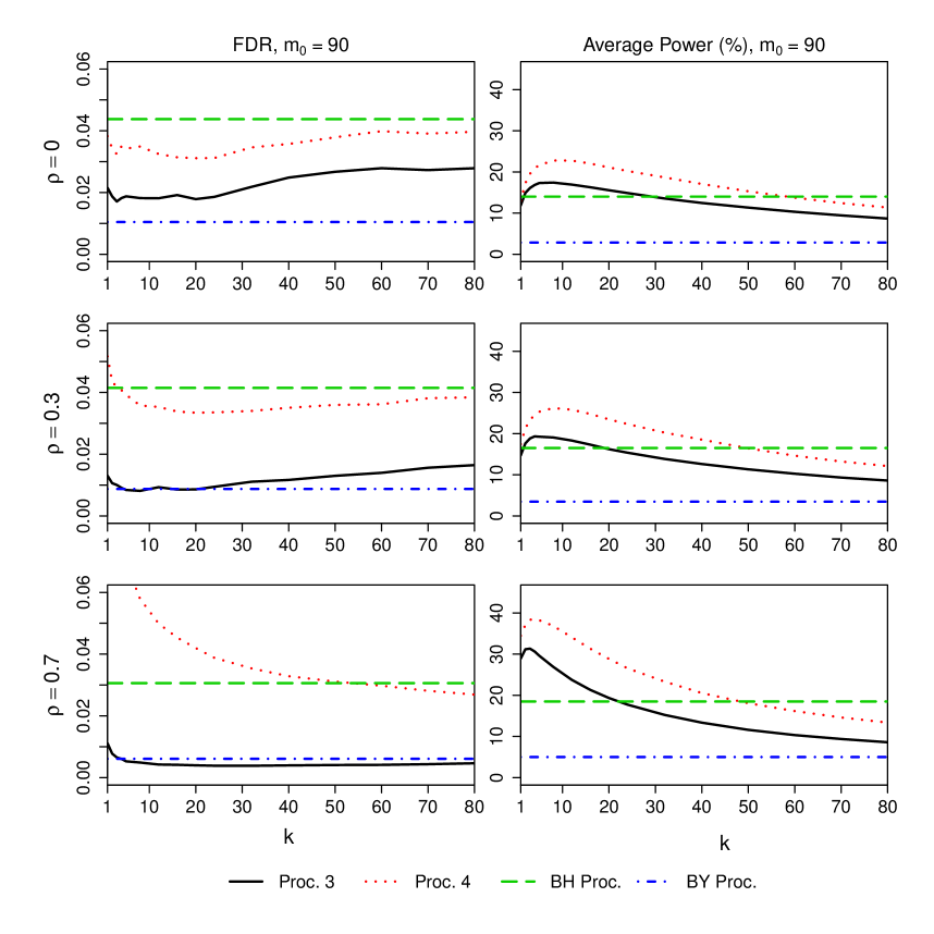
Figure 2: The FDR (left) and average power (right) of Procedure 3 (solid), Procedure 4 (dotted), the BH procedure (dashed), and the BY procedure (dotted dash) for 100 hypotheses with $m_{0}=90$ and $n=10$ under common correlation.

In each simulation, $n$ independent $m$ dimensional random normal vectors with covariance matrix $\Sigma$ and components $Z_{i}\sim N(\mu_{i},1),i=1,\dots,m$, were generated. The $p$-value for testing $H_{i}:\mu_{i}=0$ vs. $H^{\prime}_{i}:\mu_{i}>0$ was calculated using a one-sided, one-sample $t$-test for each $i$. The $\mu_{i}$ corresponding to each false null hypothesis is set to the value at which the power of one-sample t-test at level $0.05$ is $0.75$. As for the joint dependence, we considered a common correlation structure where $\Sigma$ had off-diagonal components equal to $\rho$ and diagonal components equal to 1.

We set $\alpha=0.05$ and $m=100$. The hypotheses were ordered using the ‘sum of squares ordering’ used in Example 1 from Section 5. We had 5,000 runs of simulation for each of the procedures considered. We noted the false discovery proportion and the proportion of correctly rejected false null hypotheses for each procedure in each of these runs. The simulated FDR and average power (the expected proportion of correctly rejected false null hypotheses) were obtained by averaging out the corresponding 5,000 values.

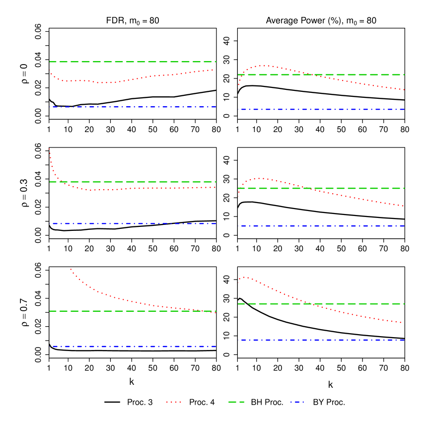
Figure 3: The FDR (left) and average power (right) of Procedure 3 (solid), Procedure 4 (dotted), the BH procedure (dashed), and the BY procedure (dotted dash) for 100 hypotheses with $m_{0}=80$ and $n=10$ under common correlation.

We first compared Procedures 1-4 with the BH and BY procedures when $m_{0}=90$ and $n=10$. Figure 2 displays these comparisons in terms of the simulated FDR and average power, respectively, under common correlation with $\rho=0$ (independence), $\rho=0.3$, and $\rho=0.7$ while $k$ varies from 1 to 80. We did not explicitly label Procedures 1 and 2 as these are both special cases of Procedures 3 and 4 when $k=1$, respectively. As seen from Figure 2, Procedure 3 controls the FDR at level $0.05$ under every dependence configuration. Procedure 4 controls the FDR under independence ($\rho=0$), generally maintains controls of the FDR under mild correlation ($\rho=0.3$), but loses control of the FDR for small values of $k$ under strong correlation ($\rho=0.7$). From Figure 2, one can also see that Procedure 3 tends to have its largest power when $k$ is between about 3 and 10, and Procedure 4 tends to have its largest power when $k$ is between about 5 and 15. In addition, Figure 2 shows that for a well chosen $k$, Procedures 3 and 4 outperform the BH procedure, and for all values of $k$, Procedures 3 and 4 outperform the BY procedure.

Next, we compared the FDR and average power of these procedures when $m_{0}=80$ and $n=10$. Figure 3 displays these comparisons for $\rho=0$, $\rho=0.3$, and $\rho=0.7$ while $k$ varies from 1 to 80. In terms of FDR, the results shown in Figure 3 are similar to the results shown in Figure 2. In terms of power, Figure 3 shows that the powers of all the procedures tend to show an increase over the powers shown in Figure 2. Figure 3 also shows that for a well chosen $k$, Procedures 4 can outperform the BH procedure, but, in general, Procedure 3 cannot. Again, for all values of $k$, Procedures 3 and 4 outperform the BY procedure.

7 Concluding Remarks

In this paper, we have developed ‘step-down’ procedures which control the FDR and exploit the structure of pre-ordered hypotheses. We have been able to produce the desired methods in the most simple as well as a general setting covering different dependence scenarios. Our simulation study and real data analysis show that in some cases, the proposed procedures can be powerful alternatives to existing FDR controlling procedures.

Using some of the techniques developed in this paper, it is possible to develop other types of fixed sequence procedures controlling the FDR, such as a fallback-type procedure. Unlike the conventional and generalized fixed sequence procedures developed in this paper, the fallback-type procedure tests the remaining hypotheses no matter how many earlier hypotheses are accepted, which is needed for analyzing stream data in sequential change detection problems.

Although we have only considered the simplest hierarchical structure – fixed sequence structure – by using the similar techniques presented in this paper, we were able to develop simple and powerful procedures that control the FDR under various dependencies when testing multiple hypotheses with a more complex hierarchical structure. We plan to present these procedures in a future communication.

Appendix

7.1 Proof of Theorem 3.1 (ii)

For any $u_{1}$, $1\leq u_{1}\leq m$, consider a joint distribution of the $p$-values such that the first $u_{1}-1$ hypotheses are false null hypotheses whose corresponding $p$-values are $0$ with probability one. The remaining $m-u_{1}+1$ hypotheses are true null hypotheses such that $\hat{P}_{1}\sim U(0,1)$ and $\hat{P}_{i}=\hat{P}_{1}$ for $i=2,\dots,m_{0}$. Under such joint distribution of the $p$-values, the FDR of the conventional fixed sequence procedure is exactly $\alpha^{(1)}_{u_{1}}(m-u_{1}+1)/m$. If $\alpha^{(1)}_{u_{1}}=1$ then the critical constant is already at its largest and cannot be improved. Otherwise, if $\alpha^{(1)}_{u_{1}}<1$, then FDR $=\alpha$ and thus $\alpha^{(1)}_{u_{1}}$ cannot be made any larger.

In the above construction $\vec{P}$ is PRDS on $\vec{P}_{0}$. We only need to note that for $i=1,\ldots,m_{0}$, $\widehat{P}_{i}=p$ implies $\vec{P}=(0,\dots,0,p,\dots,p)$. Thus, for any increasing set $D$,

$$\mathrm{Pr}\left(\vec{P}\in D|\widehat{P}_{i}=p\right)=\begin{cases}1&\text{ if }(0,\dots,0,p,\dots,p)\in D\\ 0&\text{ otherwise},\end{cases}$$

which is an increasing function in $p$.  

7.2 Proof of Lemma 3.1

Lemma 3.1 can be regarded as a special case of Lemma 4.1 with $k=1$. Note that for $i=1,\ldots,m$, $m_{1,i}=m_{1,i-1}$ and $m_{0,i}=m_{0,i-1}+1$ when $i\in I_{0}$, $m_{0,i}=m_{0,i-1}$ when $i\notin I_{0}$, and $m_{0,i-1}+m_{1,i-1}=i-1$. Thus, when $k=1$, the event $\{R\geq i\}$ implies $V_{i}=m_{0,i}$ and hence

$$\frac{V_{i}}{i}-\frac{V_{i-1}}{i-1}=\begin{cases}1_{\{1\in I_{0}\}}&\text{ for }i=1\\ \frac{m_{1,i-1}1_{\{i\in I_{0}\}}-m_{0,i-1}1_{\{i\notin I_{0}\}}}{i(i-1)}&\text{ for }i=2,\dots,m.\end{cases}$$ (7)

By (7) and Lemma 4.1, the desired result follows.  

7.3 Proof of Lemma 4.1

It is easy to see that

FDR $$= E\left(\displaystyle\sum\limits_{\begin{subarray}{c}i=1\end{subarray}}^{\begin{subarray}{c}m\end{subarray}}\frac{V_{i}}{i}1_{\{R=i\}}\right)=E\left(\displaystyle\sum\limits_{\begin{subarray}{c}i=1\end{subarray}}^{\begin{subarray}{c}m\end{subarray}}\left(\frac{V_{i}}{i}1_{\{R\geq i\}}-\frac{V_{i}}{i}1_{\{R\geq i+1\}}\right)\right)$$

$$= E\left(\displaystyle\sum\limits_{\begin{subarray}{c}i=1\end{subarray}}^{\begin{subarray}{c}m\end{subarray}}\left(\frac{V_{i}}{i}-\frac{V_{i-1}}{i-1}\right)1_{\{R\geq i\}}\right)$$

$$= E\left(\displaystyle\sum\limits_{\begin{subarray}{c}i=1\end{subarray}}^{\begin{subarray}{c}m\end{subarray}}\left(\frac{V_{i}}{i}-\frac{V_{i-1}}{i-1}\right)1_{\{J_{i}<m+1\}}\right),$$

the desired result.   

7.4 Proof of Lemma 4.2

It is easy to see that for $i=1,\ldots,m$, if there are at least $i$ rejections , then $i\leq J_{i}\leq\min(i+k-1,m)$. For ease of notation, let $j_{i}^{*}=\min(i+k-1,m)$. For $i,j=1,\ldots,m$, define $f_{i}(j)=\frac{(k-j+i)\alpha}{k}\frac{S_{i}}{i}$ and $W_{i}(j)=1_{\{J_{i-1}\leq j,J_{i}>j\}}$. Regarding the relationship between $J_{i}$ and $W_{i}(j)$, there are the following two equalities available:

$$1_{\{J_{i}=j\}}=W_{i}(j-1)1_{\{P_{j}\leq\alpha^{(4)}_{j}\}}$$ (8)

and

$$W_{i}(j)-W_{i}(j-1)=1_{\{J_{i-1}=j\}}-1_{\{J_{i}=j\}}.$$ (9)

The first equality follows from the fact that for $i=1,\ldots,m$ and $j=i,\dots,j_{i}^{*}$, when $J_{i}=j$, there are $i-1$ rejections among the first $j-1$ tested hypotheses and the $i^{th}$ rejection is exactly the $j^{th}$ tested hypothesis, thus

$$1_{\{J_{i}=j\}}=1_{\{J_{i-1}\leq j-1,J_{i}>j-1,P_{j}\leq\alpha^{(4)}_{j}\}}=W_{i}(j-1)1_{\{P_{j}\leq\alpha^{(4)}_{j}\}}.$$

The second equality follows from the fact that the event $\{W_{i}(j)=1\}$ implies that there are exactly $i-1$ rejections among the first $j$ tested hypotheses, thus for $j=i-1,\dots,j_{i-1}^{*}$,

$$W_{i}(j)-W_{i}(j-1)=1_{\{J_{i-1}\leq j,J_{i}>j\}}-W_{i}(j-1)$$

$$= 1_{\{J_{i-1}=j\}}+1_{\{J_{i-1}\leq j-1,J_{i}>j-1,P_{j}>\alpha^{(4)}_{j}\}}-W_{i}(j-1)$$

$$= 1_{\{J_{i-1}=j\}}-W_{i}(j-1)1_{\{P_{j}\leq\alpha^{(4)}_{j}\}}$$

$$= 1_{\{J_{i-1}=j\}}-1_{\{J_{i}=j\}},$$

where, the third equality follows from the fact that $1_{\{P_{j}>\alpha^{(4)}_{j}\}}=1-1_{\{P_{j}\leq\alpha^{(4)}_{j}\}}$ and the fourth follows from (8).

By using the above two equalities, we can prove two inequalities below, which are needed in the proof of this lemma. Firstly, we show by using (8) that the following inequality holds:

$$E\left(\left(\frac{V_{i}}{i}-\frac{V_{i-1}}{i-1}+f_{i}(j)-f_{i-1}(j)\right)1_{\{J_{i}=j\}}\right)\leq E\left(\frac{\alpha}{k}\frac{S_{i-1}}{i-1}W_{i}(j-1)\right).$$ (10)

Proof of (10). To see this, we consider, separately, the case when $j\in I_{0}$ and when $j\notin I_{0}$.

Suppose $j\in I_{0}$, then $S_{i}=S_{i-1}$ and $V_{i}=V_{i-1}+1$ when $J_{i}=j$. Using the fact that $V_{i-1}+S_{i-1}=i-1$, the left hand side of (10), after some algebra, becomes

$$E\left(\frac{k+(j-k)\alpha}{ki}\frac{S_{i-1}}{i-1}W_{i}(j-1)1_{\{P_{j}\leq\alpha^{(4)}_{j}\}}\right)$$

$$= E\left(\frac{k+(j-k)\alpha}{ki}\frac{S_{i-1}}{i-1}W_{i}(j-1)\right)\mathrm{Pr}\left(P_{j}\leq\alpha^{(4)}_{j}\right)$$

$$\leq E\left(\frac{k+(j-k)\alpha}{ki}\frac{S_{i-1}}{i-1}W_{i}(j-1)\right)\frac{i\alpha}{k+(j-k)\alpha}$$

$$= E\left(\frac{\alpha}{k}\frac{S_{i-1}}{i-1}W_{i}(j-1)\right).$$

The first equality follows from these two facts: (i) When $J_{i}=j$, i.e. the $i^{th}$ rejection is $H_{j}$, $S_{i-1}$ is only dependent on the first $j-1$ $p$-values, since $S_{i-1}$ is the number of false null hypotheses among the first $i-1$ rejections; (ii) $W_{i}(j-1)$ is also only dependent on the first $j-1$ $p$-values, since $W_{i}(j-1)$ is 1 if and only if there are exactly $i-1$ rejections among the first $j-1$ hypotheses tested. The inequality follows from (1).

Now suppose $j\notin I_{0}$, then $S_{i}=S_{i-1}+1$ and $V_{i}=V_{i-1}$. Similarly, using the fact that $V_{i-1}+S_{i-1}=i-1$, the left hand side of (10), after some algebra, becomes

$$E\left(\left(\frac{-V_{i-1}}{i(i-1)}+\frac{((j-k)S_{i-1}+(i-1)(k-j+i))\alpha}{ki(i-1)}\right)W_{i}(j-1)1_{\{P_{j}\leq\alpha^{(4)}_{j}\}}\right)$$

$$\leq E\left(\left(\frac{-V_{i-1}}{i(i-1)}\frac{(k-j+i)\alpha}{k}+\frac{((j-k)S_{i-1}+(i-1)(k-j+i))\alpha}{ki(i-1)}\right)W_{i}(j-1)\right)$$

$$= E\left(\frac{\alpha}{k}\frac{S_{i-1}}{i-1}W_{i}(j-1)\right).$$

The inequality follows by the fact that $j\geq i$ so that $k-j+i\leq k$. In addition, in the last line we use the fact that $V_{i-1}+S_{i-1}=i-1$.   

Next, we show by using (9) that the following inequality holds:

$$E\left(f_{i-1}(J_{i-1})1_{\{J_{i-1}<m+1\}}-f_{i-1}(J_{i})1_{\{J_{i}<m+1\}}\right)\geq E\left(\displaystyle\sum\limits_{\begin{subarray}{c}j=i\end{subarray}}^{\begin{subarray}{c}j_{i}^{*}\end{subarray}}\frac{\alpha}{k}\frac{S_{i-1}}{i-1}W_{i}(j-1)\right).$$ (11)

Proof of (11). By using (9), we have

$$\qquad E\left(f_{i-1}(J_{i-1})1_{\{J_{i-1}<m+1\}}-f_{i-1}(J_{i})1_{\{J_{i}<m+1\}}\right)$$

$$= E\left(\displaystyle\sum\limits_{\begin{subarray}{c}j=i-1\end{subarray}}^{\begin{subarray}{c}j_{i-1}^{*}\end{subarray}}f_{i-1}(j)1_{\{J_{i-1}=j\}}-\displaystyle\sum\limits_{\begin{subarray}{c}j=i\end{subarray}}^{\begin{subarray}{c}j_{i}^{*}\end{subarray}}f_{i-1}(j)1_{\{J_{i}=j\}}\right)$$

$$= E\left(\displaystyle\sum\limits_{\begin{subarray}{c}j=i-1\end{subarray}}^{\begin{subarray}{c}j_{i-1}^{*}\end{subarray}}f_{i-1}(j)1_{\{J_{i-1}=j\}}-\displaystyle\sum\limits_{\begin{subarray}{c}j=i\end{subarray}}^{\begin{subarray}{c}j_{i-1}^{*}\end{subarray}}f_{i-1}(j)1_{\{J_{i}=j\}}\right)$$

$$= E\left(\displaystyle\sum\limits_{\begin{subarray}{c}j=i\end{subarray}}^{\begin{subarray}{c}j_{i-1}^{*}\end{subarray}}f_{i-1}(j)\left(1_{\{J_{i-1}=j\}}-1_{\{J_{i}=j\}}\right)+f_{i-1}(i-1)1_{\{J_{i-1}=i-1\}}\right)$$

$$= E\left(\displaystyle\sum\limits_{\begin{subarray}{c}j=i\end{subarray}}^{\begin{subarray}{c}j_{i-1}^{*}\end{subarray}}f_{i-1}(j)(W_{i}(j)-W_{i}(j-1))+f_{i-1}(i-1)W_{i}(i-1)\right)$$

$$= E\left(\displaystyle\sum\limits_{\begin{subarray}{c}j=i\end{subarray}}^{\begin{subarray}{c}j_{i-1}^{*}\end{subarray}}\left(f_{i-1}(j-1)-f_{i-1}(j)\right)W_{i}(j-1)+f_{i-1}(j_{i-1}^{*})W_{i}(j_{i-1}^{*})\right)$$

$$\geq E\left(\displaystyle\sum\limits_{\begin{subarray}{c}j=i\end{subarray}}^{\begin{subarray}{c}j_{i}^{*}\end{subarray}}\frac{\alpha}{k}\frac{S_{i-1}}{i-1}W_{i}(j-1)\right),$$

the desired result. Here, the second equality follows from the fact that if $j_{i-1}^{*}=m$, then $j_{i}^{*}=m$; otherwise, $j_{i-1}^{*}=i+k-2$ and $j_{i}^{*}=i+k-1$ so that $f_{i-1}(j_{i}^{*})=0$. The fourth equality follows from (9) and the fact that $W_{i}(i-1)=1_{\{J_{i-1}=i-1\}}$. The inequality follows from the definition of $f_{i-1}(j)$.   

Proof of Lemma 4.2. Finally, by combining these two inequalities, we can get the desired result as follows.

$$\qquad E\left(\left(\frac{V_{i}}{i}-\frac{V_{i-1}}{i-1}\right)1_{\{J_{i}<m+1\}}\right)$$

$$= E\left(\left(\frac{V_{i}}{i}-\frac{V_{i-1}}{i-1}+f_{i}(J_{i})-f_{i-1}(J_{i})\right)1_{\{J_{i}<m+1\}}\right)$$

$$-E\left(f_{i-1}(J_{i-1})1_{\{J_{i-1}<m+1\}}-f_{i-1}(J_{i})1_{\{J_{i}<m+1\}}\right)$$

$$+E\left(f_{i-1}(J_{i-1})1_{\{J_{i-1}<m+1\}}-f_{i}(J_{i})1_{\{J_{i}<m+1\}}\right)$$

$$= E\left(\displaystyle\sum\limits_{\begin{subarray}{c}j=i\end{subarray}}^{\begin{subarray}{c}j_{i}^{*}\end{subarray}}\left(\frac{V_{i}}{i}-\frac{V_{i-1}}{i-1}+f_{i}(j)-f_{i-1}(j)\right)1_{\{J_{i}=j\}}\right)$$

$$-E\left(f_{i-1}(J_{i-1})1_{\{J_{i-1}<m+1\}}-f_{i-1}(J_{i})1_{\{J_{i}<m+1\}}\right)$$

$$+E\left(f_{i-1}(J_{i-1})1_{\{J_{i-1}<m+1\}}-f_{i}(J_{i})1_{\{J_{i}<m+1\}}\right)$$

$$\leq E\left(\displaystyle\sum\limits_{\begin{subarray}{c}j=i\end{subarray}}^{\begin{subarray}{c}j_{i}^{*}\end{subarray}}\frac{\alpha}{k}\frac{S_{i-1}}{i-1}W_{i}(j-1)-\displaystyle\sum\limits_{\begin{subarray}{c}j=i\end{subarray}}^{\begin{subarray}{c}j_{i}^{*}\end{subarray}}\frac{\alpha}{k}\frac{S_{i-1}}{i-1}W_{i}(j-1)\right)$$

$$+E\left(f_{i-1}(J_{i-1})1_{\{J_{i-1}<m+1\}}-f_{i}(J_{i})1_{\{J_{i}<m+1\}}\right)$$

$$= E\left(f_{i-1}(J_{i-1})1_{\{J_{i-1}<m+1\}}-f_{i}(J_{i})1_{\{J_{i}<m_{1}\}}\right),$$

The inequality follows from (10) and (11).

References

- [1]
- [2] Aharoni, E. and Rosset, S. (2014). Generalized a-investing: definitions, optimality results and application to public databases. Journal of the Royal Statistical Society: Series B 76 771–794.
- [3] Barber, R. and Candes, E. (2015). Controlling the false discovery rate via knockoffs. The Annals of Statistics 43 2055–2085.
- [4] Benjamini, Y. and Heller, R. (2007). False discovery rates for spatial signals. J. Amer. Satist. Assoc. 102 1272–1281.
- [5] Benjamini, Y. and Hochberg, Y. (1995). Controlling the false discovery rate: A practical and powerful approach to multiple testing. J. Roy. Statist. Soc. Ser. B 57 289–300.
- [6] Benjamini, Y. and Yekutieli, D. (2001). The control of the false discovery rate in multiple testing under dependency. Ann. Statist. 29 1165–1188.
- [7] Dmitrienko, A., D’Agostino, R., and Huque, M. (2013). Key multiplicity issues in clinical drug development. Statistics in Medicine 32 1079–1111.
- [8] Efron, B. (2008). Microarrays, empirical Bayes and the two-groups model. Statistical Science 23 1–22.
- [9] Farcomeni, A. and Finos, L. (2013). FDR control with pseudo-gatekeeping based on a possibly data driven order of the hypotheses. Biometrics 69 606–613.
- [10] Finner, H. and Roters, M. (2001). On the false discovery rate and expected type I errors. Biometrical Journal 43 985–1005
- [11] Finos, L. and Farcomeni, A. (2011). -FWER control without multiplicity correction, with application to detection of genetic determinants of multiple sclerosis in Italian twins. Biometrics 67 174–181.
- [12] Fithian, W., Taylor, J., Tibshirani, R., and Tibshirani, R. (2015). Selective Sequential Model Selection. arXiv preprint arXiv:1512.02565.
- [13] G’Sell, M. G., Wager, S., Chouldechova, A., and Tibshirani, R. (2016). Sequential selection procedures and false discovery rate control. Journal of the Royal Statistical Society: Series B 78 423–444.
- [14] Goeman, J. and Finos, L. (2012). The inheritance procedure: Multiple testing of tree-structured hypotheses. Statistical Applications in Genetics and Molecular Biology 11 1–18.
- [15] Goeman, J. and Mansmann, U. (2008). Multiple testing on the directed acyclic graph of gene ontology. Bioinformatics 24 537–544.
- [16] Goeman, J. and Solari, A. (2010). The sequential rejection principle of familywise error control. Ann. Statist. 38 3782–3810.
- [17] Guo, W. and Rao, M. (2008). On control of the false discovery rate under no assumption of dependency. Journal of Statistical Planning and Inference 28 3176–3188.
- [18] Heller, R., Manduchi, E., Grant, G., and Ewens, W. (2009). A flexible two-stage procedure for identifying gene sets that are differentially expressed. Bioinformatics 25 929–942.
- [19] Hommel, G., Bretz, F., and Maurer, W. (2007). Powerful short-cuts for multiple testing procedures with special reference to gatekeeping strategies. Statistics in Medicine 26 4063–4074.
- [20] Hommel, G. and Kropf, S. (2005). Testing for differentiation in gene expression using a data driven order or weights for hypotheses. Biometrical Journal 47 554–562.
- [21] Huque, M. and Alosh, M. (2008). A flexible fixed-sequence testing method for hierarchically ordered correlated multiple endpoints in clinical trials. Journal of Statistical Planning and Inference 138 321–335.
- [22] Javanmard, A. and Montanari, A. (2015). On online control of false discovery rate. arXiv preprint arXiv:1502.06197.
- [23] Joag Dev, K. and Proschan, F. (1983). Negative association of random variables with applications. Ann. Statist. 11 286–295.
- [24] Kropf, S. and Luter, J. (2002). Multiple tests for different sets of variables using a data-driven ordering of hypotheses, with an application to gene expression data. Biometrical Journal 44 789–800.
- [25] Kropf, S., Luter, J., Eszlinger, M., Krohn, K., and Paschkeb, R. (2004). Nonparametric multiple test procedures with data-driven order of hypotheses and with weighted hypotheses. Journal of Statistical Planning and Inference 125 31–47.
- [26] Lehmann, E. and Romano, J. (2005). Testing statistical hypotheses. Springer, New York.
- [27] Lei, L. and Fithian, W. (2016). Power of ordered hypothesis testing. arXiv preprint arXiv:1606.01969.
- [28] Li, A. and Barber, R. (2015). Accumulation tests for FDR control in ordered hypothesis testing. arXiv preprint arXiv:1505.07352 (To appear in JASA.)
- [29] Li, J. and Mehrotra, D. (2008). An efficient method for accommodating potentially underpowered primary endpoints. Statistics in Medicine 27 5377–5391.
- [30] Maurer, W., Hothorn, L., and Lehmacher, W. (1995). Multiple comparisons in drug clinical trials and preclinical assays: A-priori ordered hypotheses. Vol. 6, Fischer-Verlag, Stuttgart, Germany.
- [31] Mehrotra, D. and Heyse, J. (2004). Use of the false discovery rate for evaluating clinical safety data. Statistical Methods in Medical Research 13 227–238.
- [32] Millen, B. and Dmitrienko, A. (2011). Chain procedures: A class of flexible closed testing procedures with clinical trial applications. Statistics in Biopharmaceutical Reseach 3 14–30.
- [33] Rosenbaum, P. (2008). Testing hypotheses in order. Biometrika 95 248–252.
- [34] Ross, G. J., Tasoulis, D., and Adams, N. (2011). Nonparametric monitoring of data streams for changes in location and scale. Technometrics 53 379–389.
- [35] Sarkar, S. K. (2002). Some results on false discovery rate in stepwise multiple testing procedures. Ann. Statist. 30 239-257.
- [36] van’t Wout, A., Lehrma, G., Mikheeva, S., OKeeffe, G., Katze, M., Bumgarner, R., Geiss, G., and Mullins, J. (2003). Cellular gene expression upon human immunodeficiency virus type 1 infection of CD4(+)-T-cell lines. Journal of Virology 77 1392–1402.
- [37] Westfall, P. and Krishen, A. (2001). Optimally weighted, fixed sequence and gate-keeper multiple testing procedures. Journal of Statistical Planning and Inference 99 25–41.
- [38] Westfall, P., Kropf, S., and Finos, L. (2004). Weighted FWE-controlling methods in highdimensional situations. In Recent Developments in Multiple Comparison Procedures, eds. Y. Benjamini, F. Bretz, and S. Sarkar, Vol. 47, Beachwood, OH: Institute of Mathematical Statistics, pp. 143–154.
- [39] Wiens, B. (2003). A fixed sequence Bonferroni procedure for testing multiple endpoints. Pharmaceutical Statistics 2 211–215.
- [40] Wiens, B. and Dmitrienko, A. (2005). The fallback procedure for evaluating a single family of hypotheses. J. Biopharm. Stat. 15 929–942.
- [41] Wiens, B. and Dmitrienko, A. (2010). On selecting a multiple comparison procedure for analysis of a clinical trial: Fallback, fixed sequence, and related procedures. Statistics in Biopharmaceutical Research 2 22–32.
- [42] Yekutieli, D. (2008). Hierarchical false discovery rate-controlling methodology. J. Amer. Statist. Assoc. 103 309–316.
- [43]