Thermalization of noninteracting quantum systems coupled to blackbody radiation:
A Lindblad-based analysis

Abstract

We study the thermalization of an ensemble of $N$ elementary, arbitrarily-complex, quantum systems, mutually noninteracting but coupled as electric or magnetic dipoles to a blackbody radiation. The elementary systems can be all the same or belong to different species, distinguishable or indistinguishable, located at fixed positions or having translational degrees of freedom. Even if the energy spectra of the constituent systems are nondegenerate, as we suppose, the ensemble unavoidably presents degeneracies of the energy levels and/or of the energy gaps. We show that, due to these degeneracies, a thermalization analysis performed by the popular quantum optical master equation reveals a number of serious pathologies, possibly including a lack of ergodicity. On the other hand, a consistent thermalization scenario is obtained by introducing a Lindblad-based approach, in which the Lindblad operators, instead of being derived from a microscopic calculation, are established as the elements of an operatorial basis with squared amplitudes fixed by imposing a detailed balance condition and requiring their correspondence with the dipole transition rates evaluated under the first-order perturbation theory. Due to the above-mentioned degeneracies, this procedure suffers a basis arbitrariness which, however, can be removed by exploiting the fact that the thermalization of an ensemble of noninteracting systems cannot depend on the ensemble size. As a result, we provide a clear-cut partitioning of the thermalization time into dissipation and decoherence times, for which we derive formulas giving the dependence on the energy levels of the elementary systems, the size $N$ of the ensemble, and the temperature of the blackbody radiation.

I INTRODUCTION

The study of open quantum systems Breuer and Petruccione (2002); Schaller (2014) is crucial for a modern understanding of the foundations of quantum mechanics, and finds numerous applications in fields such as solid state physics, quantum optics, and quantum computation, where questions about decoherence and dissipation are of theoretical and practical importance. In particular, the call for nonunitary evolutions designed to perform quantum operations, like purification via, e.g., quantum adiabatic algorithms Farhi et al. (2001), or cooling via, e.g., thermalization Laumann et al. (2015), raises issues on the possibility of preparing a large system of $N$ qubits in its ground state Ticozzi and Viola (2014).

In the above and other situations, one deals with the problem of evaluating the thermalization time $\tau$ of a quantum many-body system in contact with a thermal reservoir. To be more precise, let $\bm{H}$ be the Hamiltonian of the isolated many-body system and $\bm{\rho}(t)$ its reduced density matrix operator at time $t$, when interacting with a thermal reservoir at temperature $T$. Ordinary quantum statistical mechanics postulates that, upon reaching thermal equilibrium, the system acquires two main features: (a) it becomes an incoherent mixture of its eigenstates, i.e., for $t\to\infty$, $\bm{\rho}(t)$ becomes diagonal in any eigenbasis of $\bm{H}$; and (b) the Gibbs distribution is attained, i.e., $\bm{\rho}(t)\to\bm{\rho}^{(\mathrm{eq})}=e^{-\beta\bm{H}}/\mathrm{tr}(e^{-\beta\bm{H}})$, where $\beta=1/(k_{B}T)$, $k_{B}$ being the Boltzmann constant. Two natural questions then arise: Given $T$, and given the initial density matrix operator $\bm{\rho}(0)$, how can $\bm{\rho}(t)$ evolve toward the Gibbs distribution? and What are the typical relaxation times $\tau^{(Q)}$ and $\tau^{(P)}$ required for (a) and (b) to be established, respectively?

A milestone approach to open quantum systems is provided by the Lindblad equation Lindblad (1976); Gorini et al. (1976). A crucial point in the Lindblad equation is the choice of the involved Lindblad operators. As long as these operators remain unspecified, we refer to the Lindblad class. More precisely, we have a Lindblad class for any given system characterized by its Hamiltonian $\bm{H}$. It is known that there is no Lindblad equation able to reproduce the exact evolution of $\bm{\rho}(t)$, for the dynamics of an open system is never really linear in $\bm{\rho}(t)$ Grabert (1982); Grabert and Talkner (1983). Nevertheless, a Lindblad equation can provide an effective description in terms of a coarse grained dynamics, if the correlation time of the environment is much shorter than the correlation time of the isolated system . By varying the choice of the Lindblad operators in the Lindblad class, one can span a large variety of different Lindblad equations, among which an optimal one can be found in terms of closeness to the real $\bm{\rho}(t)$ of the given system and environment. We call this method of determining the optimal Lindblad equation once the Lindblad class has been postulated, the Lindblad-based approach (LBA). The optimization procedure could require nontrivial conditions to be imposed.

Parallel to the LBA, there exists a more physically motivated method for proceeding, namely, a microscopic derivation. Given the system, the environment, and the system-environment Hamiltonians, by explicit calculations one obtains an equation for $\bm{\rho}(t)$ that belongs to the Lindblad class with the Lindblad operators fully determined. A celebrated example is the quantum optical master equation Breuer and Petruccione (2002); Schaller (2014), which describes the dipole interaction of a system with a blackbody radiation. However, in the microscopic derivation a series of approximations is introduced in order to reach an equation that belongs to the Lindblad class. Even if these approximations are physically sound, their validity is, in general, out of control. It may happen that, even if the equation resulting from the microscopic derivation belongs to the Lindblad class, it does not coincide with the Lindblad equation found in the LBA.

In this paper, we study the approach to equilibrium of an ensemble of $N$ noninteracting elementary quantum systems coupled as electric or magnetic dipoles to a blackbody radiation. As long as the interaction with the radiation can be effectively reduced to dipolar terms only, the elementary systems can be arbitrarily complex. They can be all the same or belonging to different species, distinguishable or indistinguishable, located at fixed positions or moving in a lattice or in a box. Examples range from a pure gas Jona-Lasinio et al. (2002) or a mixture Presilla and Jona-Lasinio (2015) of chiral molecules at a low density, to a chipset of superconducting flux qubits Boixo et al. (2014). Ensembles of $N$ mutually noninteracting systems are nontrivial when coupled to an environment. As far as we know, there are no explicit formulas describing their relaxation times to equilibrium when $N>1$. Note that here the problem is not merely mathematical (there are excellent methods to solve a given Lindblad equation when $\bm{H}$ is quadratic and the Lindblad operators proportional to one-body jump terms Prosen (2008); Prosen and Seligman (2010)); we are faced with the more basic problem of how to completely determine the Lindblad operators. We also compare the Lindblad equation obtained in our approach with the quantum optical master equation and show that, whereas the former provides a thermalization scenario consistent with phenomenology, the latter has pathological behaviors. This proposes the LBA also for studying interacting systems where many-body jump operators are involved Macrì et al. (2017); Ostilli and Presilla .

II METHODS

For a system with a nondegenerate energy spectrum, the LBA is relatively simple. Suppose that the system interacts with a blackbody radiation. We define an optimal Lindblad equation by three steps: (a) choose the Lindblad operators as the jump operators among all possible energy levels of the isolated system, (b) impose a detailed balance condition (existence of the Gibbs stationary state) among the squared amplitudes of these jump operators, and (c) evaluate the latter squared amplitudes as the rates for dipole transitions. The Lindblad equation obtained in this way coincides with the quantum optical master equation and respects the basic properties: (p1) the stationary state (SS) is unique, and (p2) the SS coincides with the Gibbs state.

For ensembles of $N$ noninteracting systems, even if each system has nondegenerate energy spectra, the procedure, steps (a)–(c), cannot be repeated unaltered, for the spectrum of the ensemble is degenerate (if two or more systems have equal spectra) and the eigenbasis of the ensemble Hamiltonian is not unique. When degeneracies are present, there are infinite ways to define the Lindblad operators associating them with the infinite different eigenbases. Each choice can give rise to different thermalization times. However, we can remove this arbitrariness by selecting a particular eigenbasis (and corresponding Lindblad operators) and constructing with it a Lindblad equation as above, if we impose a further obvious property: (p3) in an ensemble of $N$ equal but distinguishable noninteracting systems, the thermalization time does not depend on $N$. The resulting Lindblad equation, besides respecting (p1)-(p3), provides the following scenario. There exist two natural characteristic times, $\tau^{(P)}$, representing the time by which the system loses or gains energy, and $\tau^{(Q)}$, representing the time by which the system loses quantum coherence. We have $\tau=\max\{\tau^{(P)},\tau^{(Q)}\}$, and for $\beta$ finite and $N$ large enough we find: (p4) $\tau^{(Q)}\leq\tau^{(P)}$, (p5) $\tau^{(Q)}=O(1/N)$, and (p6) $\tau^{(P)}=O(1)$ for distinguishable systems (equal or not) and, at low enough densities, for indistinguishable systems too [note that (p5) and (p6) are consistent with (p3): $\tau=O(1)$]. We provide explicit formulas for $\tau^{(P)}$ and $\tau^{(Q)}$ in the case of distinguishable systems. Depending on the degree of degeneracy, the quantum optical master equation does not satisfy some or all of the above properties.

II.1 Lindblad-based approach

Consider a generic system described by a Hermitian Hamiltonian operator $\bm{H}$ acting on a Hilbert space $\mathscr{H}$ of dimension $M$. We assume that the eigenproblem, $\bm{H}|m\rangle=E_{m}|m\rangle$, has discrete, nondegenerate, eigenvalues. The set of the corresponding eigenstates $\{|m\rangle\}$ is an orthonormal basis in $\mathscr{H}$. We arrange the eigenvalues in ascending order $E_{1}<E_{2}<\dots<E_{M}$.

When the system is coupled to a thermal reservoir, we assume that its reduced density matrix operator $\bm{\rho}(t)$ is determined by a generic Lindblad class equation Lindblad (1976); Gorini et al. (1976)

$$\frac{\mathrm{d}\bm{\rho}}{\mathrm{d}t}=-\frac{\mathrm{i}}{\hbar}\left[\bm{H}^{\prime},\bm{\rho}\right]+\sum_{\alpha}\left(\bm{L}_{\alpha}\bm{\rho}\bm{L}^{{\dagger}}_{\alpha}-\frac{1}{2}\left\{\bm{L}^{{\dagger}}_{\alpha}\bm{L}_{\alpha},\bm{\rho}\right\}\right).$$ (1)

In this equation, the coherent part of the evolution is represented by the Hermitian operator $\bm{H}^{\prime}$, which, in general, differs from the isolated system Hamiltonian $\bm{H}$. The Lindblad, or quantum jump, operators $\bm{L}_{\alpha}$ are, for the moment, completely arbitrary. Even their number is arbitrary but can always be reduced to $M^{2}-1$ Pearle (2012).

The set of $M^{2}$ dyadic operators $\{|m\rangle\langle n|\}$ forms an orthonormal basis in the space of the operators acting on $\mathscr{H}$ equipped with the Hilbert-Schmdit scalar product $\langle\bm{O}_{1},\bm{O}_{2}\rangle=\mathrm{Tr}(\bm{O}^{\dagger}_{1}\bm{O}_{2})$. In the case of dipolar interactions, and within the first-order time-dependent perturbation theory, diagonal transitions $|n\rangle\to|n\rangle$ are forbidden Davydov (1985), so that the above set reduces to the set of the $M(M-1)$ non diagonal dyadic operators. We then identify this set as the set of the Lindblad operators of Eq. (1), namely,

$$\bm{L}_{\alpha}\to\bm{L}_{m,n}=\ell_{m,n}|m\rangle\langle n|,\qquad m\neq n.$$ (2)

The meaning of the $M^{2}$ complex coefficients $\ell_{m,n}$ is made clear soon. Note that, if the spectrum of $\bm{H}$ has degeneracies, the eigenbasis $\{|m\rangle\}$ is not unique and neither are the jump operators. In this case, one should modify definition (2) in such a way that the resulting theory is invariant under a change of the basis $\{|m\rangle\}$. We will discuss this point elsewhere.

Let us denote $\langle m|\bm{\rho}|n\rangle=\rho_{m,n}$ and $\langle m|\bm{H}^{\prime}|n\rangle=H^{\prime}_{m,n}$. On imposing that $\bm{\rho}^{(\mathrm{eq})}$ is a stationary solution of Eq. (1) with jump operators (2), namely, that property (p2) is satisfied, we get $H^{\prime}_{m,n}=E^{\prime}_{m}\delta_{m,n}$ and

$$|\ell_{m,n}|^{2}=C_{m,n}e^{-\frac{\beta}{2}(E_{m}-E_{n})},$$ (3)

with $C_{m,n}=C_{n,m}\geq 0$; see Appendix A for details. It follows that the $M$ diagonal elements $\rho_{m,m}$ have an evolution decoupled from that of the $M(M-1)$ off-diagonal terms $\rho_{m,n}$, $m\neq n$, which, in turn, are decoupled from each other Alicki and Lendi (2007).

On defining $\bm{p}$ as the $M$-dimensional vector with components $p_{m}=\rho_{m,m}$, we have the Pauli equation Pauli (1928)

$$\mathrm{d}\bm{p}(t)/\mathrm{d}t=-\bm{A}\ \bm{p}(t),$$ (4)

where $\bm{A}$ is the $M\times M$ matrix with components

$$A_{m,n}=B_{m}\delta_{m,n}-|\ell_{m,n}|^{2},$$ (5)

$$B_{m}=\sum_{j}|\ell_{j,m}|^{2}.$$ (6)

Equation (4) is a master equation for the populations $p_{m}$, $\mathrm{d}p_{m}/\mathrm{d}t=\sum_{n}\left[p_{n}W_{n\to m}-p_{m}W_{m\to n}\right]$, with probability rates $W_{m\to n}=|\ell_{n,m}|^{2}$. We conclude that $|\ell_{n,m}|^{2}$ represents the probability rate of the $|m\rangle\to|n\rangle$ transition’s occurring as a consequence of the interaction with the reservoir. In the weak-coupling limit, these rates can be calculated using the time-dependent perturbation theory. In this way, the matrix elements $C_{m,n}$ of Eq. (3) can be fully determined.

The $M(M-1)$ off-diagonal elements of $\bm{\rho}$ evolve independently of each other as

$$\mathrm{d}\rho_{m,n}(t)/\mathrm{d}{t}=-\mu_{m,n}\rho_{m,n}(t),\qquad m\neq n,$$ (7)

i.e., they relax to 0 at rates

$$\mu_{m,n}=\frac{\mathrm{i}}{\hbar}(E^{\prime}_{m}-E^{\prime}_{n})+\frac{1}{2}\left(B_{m}+B_{n}\right).$$ (8)

II.2 Thermalization time

The characteristic relaxation time by which $\bm{\rho}(t)$ approaches $\bm{\rho}^{(\mathrm{eq})}$—the thermalization time, for brevity—depends on both Eq. (4) and Eq. (7).

The evolution described by Eq. (4) is determined by the spectrum of the matrix $\bm{A}$. One can prove Ostilli and Presilla some general properties of $\bm{A}$, independently of the particular values assumed by the matrix elements $C_{m,n}$. First of all, $\bm{A}$ is diagonalizable and has $M$ real eigenvalues, possibly degenerate. It certainly has a zero eigenvalue corresponding to the imposed stationary solution, by virtue of $\sum_{m}A_{m,n}=0$, a manifestation of the fact that $\mathrm{tr}\bm{\rho}(t)$ is constant. Under fair conditions of the elements $C_{m,n}$, which are expected to hold true for a nondegenerate $\bm{H}$, this eigenvalue is nondegenerate, i.e., property (p1) is satisfied, whereas all the other eigenvalues are positive. In conclusion, the $M$ eigenvalues of $\bm{A}$ can be ordered as $0=\mu_{1}(\bm{A})<\mu_{2}(\bm{A})\leq\ldots\leq\mu_{M}(\bm{A})$, and the relaxation time characterizing Eq. (4) is $1/\mu_{2}(\bm{A})$.

Concerning the relaxation times of the off-diagonal elements $\rho_{m,n}$, $m\neq n$, as stated by Eq. (8), these are trivially given by $1/\mathop{\rm Re}\mu_{m,n}$. The largest among these times is $2/\min_{m\neq n}\{B_{m}+B_{n}\}=2/(B_{(1)}+B_{(2)})$, where $B_{(k)}$ indicates the $k$th smallest value among the set $\{B_{1},B_{2},\dots,B_{M}\}$.

We conclude that the thermalization time $\tau$ of our system can be defined as

$$\tau=\max\left\{\tau^{(P)},\tau^{(Q)}\right\}, \quad\mbox{thermalization time};$$ (9a)

$$\tau^{(P)}=1/\mu_{2}(\bm{A}), \quad\mbox{dissipation time};$$ (9b)

$$\tau^{(Q)}=2/\left(B_{(1)}+B_{(2)}\right), \quad\mbox{decoherence time}.$$ (9c)

The natural interpretation is that $\tau^{(P)}$ represents a characteristic time by which the system exchanges energy with the environment, whereas $\tau^{(Q)}$ represents a characteristic time by which the system loses quantum coherence due to the interaction with the environment.

III RESULTS AND DISCUSSION

III.1 Coupling a single system to blackbody radiation

We can apply the above general scheme to the case in which the environment is a blackbody radiation and the system consists of $K$ qubits (spin $1/2$). The system-environment interaction is mediated by emission and absorption of photons via the (squared) dipole matrix elements $D_{m,n}$. By using $|\ell_{n,m}|^{2}=W_{m\to n}$, we have Davydov (1985)

$$C_{m,n}=D_{m,n}\frac{|E_{m}-E_{n}|^{3}}{2\sinh\left(\frac{\beta}{2}|E_{m}-E_{n}|\right)},$$ (10)

with

$$D_{m,n} =\gamma\sum_{h=x,y,z}\left|\langle m|\sum_{i=1}^{K}\sigma_{i}^{h}|n\rangle\right|^{2},\quad\gamma=\frac{4\mu^{2}}{3\hbar^{4}c^{3}}.$$ (11)

Note that $C_{m,m}=0$. Equation (11) is obtained supposing that the size of the system is small with respect to the radiation length $2\pi\hbar c/|E_{m}-E_{n}|$, so that a fully coherent interaction between spins and radiation takes place. More general expressions can be adopted for partially or fully incoherent interactions Ostilli and Presilla (2016).

III.2 Coupling $N$ distinguishable noninteracting systems to blackbody radiation

We now focus on the thermalization of an ensemble of $N$ systems, mutually noninteracting and distinguishable. For simplicity, we consider all equal systems, the results being easily generalized to mixtures. Let us examine in detail the case $N=2$. The Hamiltonian of the ensemble is $\bm{H}^{(2)}=\bm{H}\otimes\bm{I}+\bm{I}\otimes\bm{H}$, where $\bm{H}$ is the $M\times M$ Hamiltonian matrix of the single system having a nondegenerate spectrum and $\bm{I}$ the $M\times M$ identity matrix. We have $\bm{H}^{(2)}|m,n\rangle=E_{m,n}|m,n\rangle$ with $E_{m,n}=E_{m}+E_{n}$ and $|m,n\rangle=|m\rangle\otimes|n\rangle$. Note that the eigenvalues of $\bm{H}^{(2)}$ are degenerate, even if those of $\bm{H}$ are not. It follows that we could choose orthonormal systems of eigenvectors different from $\{|m,n\rangle\}$. For instance, we have $E_{m,n}=E_{n,m}$ and the corresponding subspace spanned by $|m,n\rangle$ and $|n,m\rangle$, could be equivalently spanned by the Bell states $(|m,n\rangle\pm|n,m\rangle)/\sqrt{2}$. However, this new eigenbasis, as well as any other eigenbasis with the exception of the product states $\{|m,n\rangle\}$, would introduce an effective system-system correlation leading to a violation of property (p3). This will be explicit in the decoupling of Eq. (16), below, which can take place only for the basis $\{|m,n\rangle\}$. We conclude that $\{|m,n\rangle\}$ is the unique eigenbasis of $\bm{H}^{(2)}$ in which (p3) can be satisfied, and the LBA applied as before.

In parallel to Eq. (2), we now choose jump operators

$$\bm{L}_{\alpha}\to\bm{L}_{m,n;p,q}=\ell_{m,n;p,q}|m,n\rangle\langle p,q|.$$ (12)

On imposing that the reduced density matrix operator of the ensemble is the Gibbs SS $e^{-\beta\bm{H}^{(2)}}/\mathrm{tr}(e^{-\beta\bm{H}^{(2)}})$, everything follows as in the case of a single system, just doubling the eigenstate indices. We have $|\ell_{m,n;p,q}|^{2}=C_{m,n;p,q}e^{-\frac{\beta}{2}(E_{m,n}-E_{p,q})}$ with $C_{m,n;p,q}=C_{p,q;m,n}\geq 0$. The diagonal elements $\rho_{m,n;m,n}$ evolve according to a Pauli equation analogous to Eq. (4) with a matrix $\bm{A}^{(2)}$ having components

$$A^{(2)}_{m,n;p,q}=B_{m,n}\delta_{m,p}\delta_{n,q}-|\ell_{m,n;p,q}|^{2},$$ (13)

$$B_{m,n}=\sum_{j,k}|\ell_{j,k;m,n}|^{2}.$$ (14)

The off-diagonal elements $\rho_{m,n;p,q}$, $m\neq p$ or $n\neq q$, evolve according to equations analogous to Eq. (7) at rates

$$\mu_{m,n;p,q}=\frac{\mathrm{i}}{\hbar}(E^{\prime}_{m,n}-E^{\prime}_{p,q})+\frac{1}{2}\left(B_{m,n}+B_{p,q}\right).$$ (15)

In the case of $N=2$ systems, each consisting of $K$ qubits coupled to a blackbody radiation, the matrix elements $C_{m,n;p,q}$ are given by an expression analogous to Eq. (10) with $D_{m,n;p,q}=\gamma\sum_{h=x,y,z}(|\langle m,n|\sum_{i=1}^{K}\sigma_{i}^{h}|p,q\rangle|^{2}+|\langle m,n|\sum_{i=K+1}^{2K}\sigma_{i}^{h}|p,q\rangle|^{2})$. It can be shown that this decomposition holds actually in a generic eigenbasis of $\bm{H}$ if we assume that the spin-radiation interaction is coherent within each system but the systems are at a distance larger than the radiation length Ostilli and Presilla (2016).

In the basis $\{|m,n\rangle\}$, the dipole elements $D_{m,n;p,q}$ (independently of their form: coherent, incoherent or mixed) admit a system-index decoupling and we have

$$C_{m,n;p,q}=C_{m,p}\delta_{n,q}+C_{n,q}\delta_{m,p},$$ (16)

where $C_{m,n}$ are the single-system nonnegative symmetric matrix elements, (10). Equation (16) also implies that $B_{m,n}=B_{m}+B_{n}$. It follows that $\bm{A}^{(2)}=\bm{A}\otimes\bm{I}+\bm{I}\otimes\bm{A}$. It is easy to check that no eigenbasis other than $\{|m,n\rangle\}$ permits this reduction. For example, in the case of the Bell states, in place of Eq. (16) we would have $C_{m,n;p,q}=(C_{m,p}\delta_{n,q}+C_{n,q}\delta_{m,p}+C_{m,q}\delta_{n,p}+C_{n,p}\delta_{m,q})/2$. Whereas Eq. (16) corresponds to one-body jump operators $\bm{L}_{m,n;p,q}$, the latter expression corresponds to a mixture of two one-body jump operators where $\bm{A}^{(2)}\neq\bm{A}\otimes\bm{I}+\bm{I}\otimes\bm{A}$.

The matrix $\bm{A}^{(2)}=\bm{A}\otimes\bm{I}+\bm{I}\otimes\bm{A}$ has $M^{2}$ eigenvalues related to the $M$ eigenvalues of the single-system matrix $\bm{A}$ by

$$\mu_{j,k}(\bm{A}^{(2)})=\mu_{j}(\bm{A})+\mu_{k}(\bm{A}),\quad j,k=1,2,\dots,M.$$ (17)

Since $\mu_{1}(\bm{A})=0$ is nondegenerate, $\bm{A}^{(2)}$ has a unique zero eigenvalue. All the other eigenvalues of $\bm{A}^{(2)}$ are positive, and the smallest one of them coincides with $\mu_{2}(\bm{A})$. This smallest non zero eigenvalue of $\bm{A}^{(2)}$ is $2d$-fold degenerate, if $d$ is the degeneracy of $\mu_{2}(\bm{A})$.

From Eq. (15) we get

$$\min_{m\neq p\ \mathrm{or}\ n\neq q}\mathop{\rm Re}\mu_{m,n;p,q}=3B_{(1)}+B_{(2)}.$$ (18)

The above analysis is straightforwardly extended to an ensemble of $N$ all equal systems with Hamiltonian $\bm{H}^{(N)}=(\bm{H}\otimes\bm{I}\otimes\dots\otimes\bm{I})+(\bm{I}\otimes\bm{H}\otimes\dots\otimes\bm{I})+\dots+(\bm{I}\otimes\bm{I}\otimes\dots\otimes\bm{H})$. The result is: $\tau^{(P)}=1/\mu_{2}(\bm{A})$ independent of $N$, and $\tau^{(Q)}=2/((2N-1)B_{(1)}+B_{(2)})$, decreasing as $1/N$. For a sufficiently large $N$ and finite temperature, we have $\tau=\max\{\tau^{(P)},\tau^{(Q}\}=\tau^{(P)}$, independent of $N$.

III.3 Free spins in a magnetic field

As an example, consider a system of $N$ independent spins located at different fixed positions, in the presence of a uniform magnetic field of strength $\Gamma$ oriented along the $x$ axis. The Hamiltonian of the single spin is $\bm{H}=-\Gamma\sigma^{x}$ and has a nondegenerate spectrum, namely, $E_{1}=-\Gamma$ and $E_{2}=\Gamma$ with eigenvectors $|1\rangle=|+\rangle$ and $|2\rangle=|-\rangle$, where $\sigma^{x}|\pm\rangle=\pm|\pm\rangle$. We have $D_{1,2}=D_{2,1}=2\gamma$ and $C_{1,2}=C_{2,1}=2\gamma(2\Gamma)^{3}/(e^{\beta\Gamma}-e^{-\beta\Gamma})$, which lead to

$$\bm{A}=\frac{2\gamma(2\Gamma)^{3}}{e^{\beta\Gamma}-e^{-\beta\Gamma}}\left(\begin{array}[]{cc}e^{-\beta\Gamma}&-e^{\beta\Gamma}\\ -e^{-\beta\Gamma}&e^{\beta\Gamma}\end{array}\right).$$ (21)

The two eigenvalues of $\bm{A}$, both nondegenerate, are $\mu_{1}(\bm{A})=0$ and $\mu_{2}(\bm{A})=(2\gamma(2\Gamma)^{3})/\tanh(\beta\Gamma)$. Since the $N$ spins are distinguishable by virtue of their different fixed position, we conclude that

$$\tau^{(P)} =\frac{\tanh(\beta\Gamma)}{2\gamma(2\Gamma)^{3}},$$ (22)

$$\tau^{(Q)} =\frac{\sinh(\beta\Gamma)}{\gamma(2\Gamma)^{3}\left(\sinh(\beta\Gamma)+Ne^{-\beta\Gamma}\right)}.$$ (23)

As a further example of independent systems with different spectra, in Appendix B we provide the expressions of $\tau^{(P)}$ and $\tau^{(Q)}$ for the above ensemble of $N$ spins in a spatially periodic magnetic field. In this case, $\tau^{(P)}$ becomes independent of $N$ only for $N$ large.

III.4 Coupling $N$ indistinguishable noninteracting systems to blackbody radiation

In this case, the laws of quantum mechanics select either totally symmetric or totally anti-symmetric eigenvectors, if the systems are bosonic or fermionic, respectively. As a consequence, the degeneracy of the spectrum of $\bm{H}^{(N)}$ is greatly reduced even if not completely eliminated. Consider, for example, a system (bosonic or fermionic) whose Hamiltonian $\bm{H}$ has four levels $E_{1}<E_{2}<E_{3}<E_{4}$ such that $E_{1}+E_{4}=E_{2}+E_{3}$. The Hamiltonian $\bm{H}^{(2)}$ of the ensemble has symmetrized or antisymmetrized eigenvectors which are twofold degenerate. However, the origin of this degeneracy is different from that of the unavoidable degeneracies which appear for distinguishable systems. It is due to the occurrence of particular relations among the levels of $\bm{H}$, which have to be regarded as rather uncommon. Typically, the basis of $\bm{H}^{(N)}$ is unique and the LBA well defined. As observed, however, this unique eigenbasis is not made by product states of single-system eigenstates, and, from what we have learned in the case of distinguishable systems, only (p1) and (p2) can be satisfied, whereas $\tau$ can be independent of $N$ only in the limit of low densities. Yet, property (p4) holds unchanged Ostilli and Presilla , and we expect that also (p5) and (p6) still apply.

Pathologies of the microscopic derivation. In the Lindblad equation resulting from the microscopic derivation, for an ensemble of $N$ noninteracting systems described by the Hamiltonian $\bm{H}^{(N)}$, instead of Eq. (2) one has (see Eqs. (3.120) and (3.143) in Ref. Breuer and Petruccione (2002))

$$\bm{L}_{\alpha}\to\bm{A}(\omega)=\sum_{\overset{m^{(N)},n^{(N)}:}{E_{n^{(N)}}-E_{m^{(N)}}=\hbar\omega}}A_{m^{(N)},n^{(N)}}|m^{(N)}\rangle\langle n^{(N)}|,$$ (24)

where $\bm{H}^{(N)}|m^{(N)}\rangle=E_{m^{(N)}}|m^{(N)}\rangle$. The symbol $\bm{A}(\omega)$ is borrowed from Breuer and Petruccione (2002) and should not be confused with the matrix $\bm{A}$ used before in our Pauli equation. Note that, even in the presence of level degeneracies, the basis $\{|m^{(N)}\rangle\}$ used in Eq. (24) is arbitrary. In fact, the operator $\bm{A}(\omega)$ is invariant with respect to a change of the eigenvectors of $\bm{H}^{(N)}$. For simplicity, let us focus on $N=2$ noninteracting, equal but distinguishable, systems, each having a nondegenerate spectrum with two levels, $E_{1}<E_{2}$. As the eigenbasis to be used in Eq. (24), let us choose the product eigenstates, $|m^{(2)}\rangle=|m,n\rangle=|m\rangle\otimes|n\rangle$, with $m,n\in\{1,2\}$. There are only two possible positive values of $\omega$ (and two corresponding negative values for which identical considerations hold): $\hbar\omega_{1}=E_{2}-E_{1}$ and $\hbar\omega_{2}=2(E_{2}-E_{1})$. Whereas for the latter we have $\bm{A}(\omega_{2})=A_{1,1;2,2}|1,1\rangle\langle 2,2|$, for the former we find $\bm{A}(\omega_{1})=A_{1,1;1,2}|1,1\rangle\langle 1,2|+A_{1,1;2,1}|1,1\rangle\langle 2,1|+A_{1,2;2,2}|1,2\rangle\langle 2,2|+A_{2,1;2,2}|2,1\rangle\langle 2,2|$. We see that each Lindblad operator $\bm{A}(\omega)$ can be the sum of more dyadic operators and this happens in correspondence with level degeneracies. By a similar example with three energy levels, it is easy to see that also gap degeneracies lead to extra dyadic operators. In other words, Eq. (24) introduces correlations among the single-system eigenstates which can lead to violations of properties (p1)–(p3). Ultimately, these correlations are an artifact due to the approximations used in the microscopic derivation.

In the most general case of $N$ distinguishable systems, possibly also different, the Lindblad equation obtained in our LBA, coincides with the Lindblad equation of the microscopic derivation only when both the conditions $\delta_{E_{m},E_{n},}=\delta_{m,n}$ and $\delta_{E_{m}-E_{n},E_{p}-E_{q}}=\delta_{m,p}\delta_{n,q}$ are met. These two conditions ensure that there are no level or gap degeneracies. Following Ref. Zhang et al. (2016), these can be interpreted as the conditions required for the isolated many-body system represented by the Hamiltonian $\bm{H}^{(N)}$ to be ergodic and mixing, respectively. These conditions are never satisfied in the case of $N>1$ equal systems. In Appendix B we provide a detailed comparison, also with numerical examples, between the quantum optical master equation, which is the Lindblad equation obtained in the microscopic derivation when the environment is a blackbody radiation, and the corresponding Lindblad equation obtained within our approach.

In the case of indistinguishable noninteracting systems, even if we exclude accidental degeneracies, in Eq. (24) we still have extra terms as soon as there are gap degeneracies, and it is easy to see that, for bosons, the latter always occur. An extended analysis of the case of indistinguishable systems will be reported elsewhere.

IV CONCLUSION

In conclusion, we have first considered the thermalization of arbitrary systems with a nondegenerate spectrum and in contact with a thermal reservoir. The analysis is done by using a Lindblad-based approach in which the Lindblad operators, initially chosen as a completely general basis set, are next fixed by requiring the existence of a Gibbs stationary state. This approach allows us to clearly identify two characteristic times $\tau^{(P)}$ and $\tau^{(Q)}$, namely, the dissipation and decoherence times, the largest of which determines the thermalization time. We have then applied this procedure to ensembles of $N$ mutually noninteracting subsystems coupled to a blackbody radiation and found explicit formulas for $\tau^{(P)}$ and $\tau^{(Q)}$. For ensembles of distinguishable subsystems, the approach must be equipped with the phenomenological condition that the thermalization time should not depend on the ensemble size $N$, which leads to complete determination of the Lindblad operators despite the exchange degeneracies. The thermalization of $N$ free spins in a magnetic field, uniform or not, coupled to a blackbody radiation, has been considered in detail. For this system, techniques for solving the Lindblad equation like those in Prosen (2008) and Prosen and Seligman (2010) are inapplicable , yet it is straightforwardly and consistently worked out by our approach. An analysis of the same system within the quantum optical master equation reveals serious physical inconsistencies.

Appendix A Lindblad-based approach to thermalization

Let us denote $\langle m|\bm{\rho}|n\rangle=\rho_{m,n}$ and $\langle m|\bm{H}^{\prime}|n\rangle=H^{\prime}_{m,n}$, with $\bm{H}|m\rangle=E_{m}|m\rangle$. Equation (1), with the choice of (2), becomes

$$\frac{\mathrm{d}\rho_{m,n}}{\mathrm{d}t}= -\frac{\mathrm{i}}{\hbar}\sum_{k}\left(H^{\prime}_{m,k}\rho_{k,n}-\rho_{m,k}H^{\prime}_{k,n}\right)+\sum_{k}\left(\left|\ell_{m,k}\right|^{2}\rho_{k,k}\delta_{m,n}-\frac{1}{2}\left|\ell_{k,m}\right|^{2}\rho_{m,n}-\frac{1}{2}\left|\ell_{k,n}\right|^{2}\rho_{m,n}\right).$$ (25)

On imposing that $\bm{\rho}^{(\mathrm{eq})}=e^{-\beta\bm{H}}/\mathrm{tr}(e^{-\beta\bm{H}})$ is a stationary solution of Eq. (25), we get

$$0= -\frac{\mathrm{i}}{\hbar}\left(H^{\prime}_{m,n}e^{-\beta E_{n}}-e^{-\beta E_{m}}H^{\prime}_{m,n}\right)+\sum_{k}\left(\left|\ell_{m,k}\right|^{2}e^{-\beta E_{k}}-\left|\ell_{k,m}\right|^{2}e^{-\beta E_{m}}\right)\delta_{m,n}.$$ (26)

For $m\neq n$, since $E_{m}\neq E_{n}$, Eq. (26) implies that $H^{\prime}_{m,n}=0$. We thus infer that $H^{\prime}_{m,n}=E^{\prime}_{m}\delta_{m,n}$, with $E^{\prime}_{m}$ real as ${\bm{H}^{\prime}}^{\dagger}=\bm{H}^{\prime}$. In other words, $\bm{H}^{\prime}$ is diagonal in the basis of the eigenvectors of $\bm{H}$. We still ignore the eigenvalues $E^{\prime}_{m}$ but this is not relevant for determining the relaxation time to equilibrium.

For $m=n$, the purely imaginary term on the right-hand side of Eq. (26) vanishes and we deduce that the coefficients $\ell_{m,n}$ must satisfy the balance condition

$$\sum_{k}\left|\ell_{m,k}\right|^{2}e^{-\beta E_{k}}=\sum_{k}\left|\ell_{k,m}\right|^{2}e^{-\beta E_{m}}.$$ (27)

The most general detailed-balance solution of Eq. (27) can be written as

$$|\ell_{m,n}|^{2}=C_{m,n}e^{-\frac{\beta}{2}(E_{m}-E_{n})},$$ (28)

provided $C_{m,n}=C_{n,m}\geq 0$.

We conclude that the elements $\rho_{m,n}$ of the reduced density matrix of the system evolve according to the following system of equations

$$\frac{\mathrm{d}\rho_{m,n}}{\mathrm{d}{t}}=\left[-\frac{\mathrm{i}}{\hbar}(E^{\prime}_{m}-E^{\prime}_{n})-\frac{1}{2}\sum_{k}\left(|\ell_{k,m}|^{2}+|\ell_{k,n}|^{2}\right)\right]\rho_{m,n}+\sum_{k}|\ell_{m,k}|^{2}\rho_{k,k}\delta_{m,n}.$$ (29)

It follows that the evolution of the diagonal components $\rho_{m,m}$ is decoupled from that of the off-diagonal elements, and the latter are also decoupled fromeach other:

$$\frac{\mathrm{d}\rho_{m,m}}{\mathrm{d}{t}}=-\left(\sum_{k}|\ell_{k,m}|^{2}\right)\rho_{m,m}+\sum_{k}|\ell_{m,k}|^{2}\rho_{k,k},$$ (30)

$$\frac{\mathrm{d}\rho_{m,n}}{\mathrm{d}{t}}=\left[-\frac{\mathrm{i}}{\hbar}(E^{\prime}_{m}-E^{\prime}_{n})-\frac{1}{2}\sum_{k}\left(|\ell_{k,m}|^{2}+|\ell_{k,n}|^{2}\right)\right]\rho_{m,n},\qquad m\neq n.$$ (31)

Appendix B Coupling with blackbody radiation: Lindblad-based approach vs microscopic derivation

Equation (29), customized with $|\ell_{m,n}|^{2}=C_{m,n}e^{-\frac{\beta}{2}(E_{m}-E_{n})}$ and the coefficients $C_{m,n}$ given in Eq. (10), is the optimal Lindblad equation obtained within our LBA in the case of coupling with a blackbody radiation. Explicitly, this equation reads

$$\frac{\mathrm{d}\rho_{m,n}}{\mathrm{d}{t}}= -\frac{\mathrm{i}}{\hbar}(E^{\prime}_{m}-E^{\prime}_{n})\rho_{m,n}$$

$$-\frac{1}{2}\sum_{k}\left(D_{k,m}\widetilde{W}_{k,m}+D_{k,n}\widetilde{W}_{k,n}\right)\rho_{m,n}$$

$$+\sum_{k}D_{m,k}\widetilde{W}_{m,k}\rho_{k,k}\delta_{m,n},$$ (32)

where

$$\widetilde{W}_{m,k}=|E_{m}-E_{k}|^{3}\frac{e^{-\frac{\beta}{2}(E_{m}-E_{k})}}{e^{\frac{\beta}{2}|E_{m}-E_{k}|}-e^{-\frac{\beta}{2}|E_{m}-E_{k}|}}.$$ (33)

For a system of $N$ qubits, the (squared) dipole matrix elements $D_{m,n}$ evaluated in the fully coherent limit are

$$D_{m,n}=\frac{4\mu^{2}}{3\hbar^{4}c^{3}}\sum_{h=x,y,z}\left|\langle m|\sum_{i=1}^{N}\sigma_{i}^{h}|n\rangle\right|^{2}.$$ (34)

Expressions more general than Eq. (34) can be adopted, depending on the size of the system; see Ref. Ostilli and Presilla (2016).

In the microscopic derivation, the coupling of a system with a blackbody radiation is described by the celebrated quantum optical master equation Breuer and Petruccione (2002); see also Schaller (2014) for an alternative derivation. This equation presents some differences with respect to the LBA, Eq. (B). Consider Eq. (3.206) in Ref. Breuer and Petruccione (2002), which provides a general quantum optical master equation in the Lindblad operatorial form and in the interaction picture. Switching to the Schrödinger picture and taking the matrix element of the corresponding operators between eigenstates $|m\rangle$ and $|n\rangle$ of the same $\bm{H}$ considered above, we get

$$\frac{\mathrm{d}\rho_{m,n}}{\mathrm{d}{t}}= -\frac{\mathrm{i}}{\hbar}(E_{m}-E_{n})\rho_{m,n}$$

$$-\frac{\mathrm{i}}{\hbar}\sum_{k,j}\left[\left(\hbar S(E_{m}-E_{k})\sum_{h=x,y,z}d^{(h)}_{k,j}\overline{d^{(h)}_{k,m}}\right)\rho_{j,n}\delta_{E_{j},E_{m}}-\left(\hbar S(E_{n}-E_{k})\sum_{h=x,y,z}d^{(h)}_{k,n}\overline{d^{(h)}_{k,j}}\right)\rho_{m,j}\delta_{E_{j},E_{n}}\right]$$

$$-\frac{1}{2}\sum_{k,j}\left[\left(\frac{4\mu^{2}}{3\hbar^{4}c^{3}}\sum_{h=x,y,z}d^{(h)}_{k,j}\overline{d^{(h)}_{k,m}}\right)\widetilde{W}_{k,m}\rho_{j,n}\delta_{E_{j},E_{m}}+\left(\frac{4\mu^{2}}{3\hbar^{4}c^{3}}\sum_{h=x,y,z}d^{(h)}_{k,n}\overline{d^{(h)}_{k,j}}\right)\widetilde{W}_{k,n}\rho_{m,j}\delta_{E_{j},E_{n}}\right]$$

$$+\sum_{k,j}\left(\frac{4\mu^{2}}{3\hbar^{4}c^{3}}\sum_{h=x,y,z}d^{(h)}_{m,k}\overline{d^{(h)}_{n,j}}\right)\widetilde{W}_{m,k}\rho_{k,j}\delta_{E_{k}-E_{m},E_{j}-E_{n}},$$ (35)

where

$$S(E)=\frac{2\mu^{2}|E|^{3}}{3\pi\hbar^{4}c^{3}}\mathrm{PV}\int_{0}^{\infty}\left(\frac{u^{3}}{1-e^{-\beta Eu}}~{}\frac{1}{1-u}+\frac{u^{3}}{e^{\beta Eu}-1}~{}\frac{1}{1+u}\right)\mathrm{d}{u}$$ (36)

and

$$d^{(h)}_{m,n}=\langle m|\sum_{i=1}^{N}\sigma_{i}^{h}|n\rangle.$$ (37)

First, we observe that in the quantum optical master equation the contribution from the Lamb shift Hamiltonian is given explicitly by the second line of Eq. (B). This term, which in general is not diagonal in the basis $\{|m\rangle\}$ due to the presence of the two Kronecker deltas, $\delta_{E_{j},E_{m}}\neq\delta_{j,m}$ and $\delta_{E_{j},E_{n}}\neq\delta_{j,n}$, is given in terms of the Cauchy principal value of the integral (36). The integral presents an ultraviolet ($u\to\infty$) divergence, presumably introduced by the approximations used to derive the quantum optical master equation. To meaningfully compare Eq. (B) with Eq. (B), we neglect the Lamb shift correction to the levels of $\bm{H}$. This amounts to disregarding the entire second line of Eq. (B) and putting $E_{m}^{\prime}=E_{m}$ in Eq. (B). As far as Eq. (B) is concerned, we have proven that such a change does not alter the relaxation time to equilibrium, since neither $\tau^{(P)}$ nor $\tau^{(Q)}$ depends on $E^{\prime}_{m}$.

If the eigenvalues of $\bm{H}$ satisfy

$$\delta_{E_{j},E_{m}}=\delta_{j,m}$$ (38)

and

$$\delta_{E_{k}-E_{m},E_{j}-E_{n}}=\delta_{k,j}\delta_{m,n},$$ (39)

Eq. (B) reduces to Eq. (B) with the coefficients $D_{m,n}$ evaluated in the fully coherent limit given by Eq. (34) To the best of our knowledge, Eq. (B) is known only in a formulation compatible with a fully coherent dipole interaction, i.e., a formulation valid when the $N$ qubits are at reciprocal distances shorter than the radiation lengths $2\pi\hbar c/|E_{m}-E_{n}|$.

If the only condition (38) is satisfied, Eq. (B) splits into a Pauli equation for the $M$ diagonal terms $\rho_{m,m}$, which is identical to the Pauli equation obtained in the LBA, and a set of equations for the off-diagonal terms $\rho_{m,n}$, $m\neq n$. In fact, in this case, for $m=n$ we have $\delta_{E_{k}-E_{m},E_{j}-E_{n}}=\delta_{E_{k},E_{j}}=\delta_{k,j}$ and the last line of Eq. (B) coincides with the last term of Eq. (B), whereas for $m\neq n$, i.e., $E_{m}\neq E_{n}$, $\delta_{E_{k}-E_{m},E_{j}-E_{n}}$ implies that $E_{k}\neq E_{j}$ and, therefore, $k\neq j$. However, unlike the equations obtained in the LBA, the $M(M-1)$ equations for the off-diagonal elements of $\bm{\rho}$ are mutually coupled. In Fig. 1 we show examples of possible arrangements of four energy levels which satisfy Eq. (38) but violate Eq. (39).

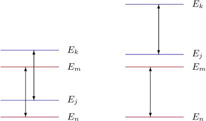
Figure 1: (Color online) Two possible arrangements of the four energy levels $E_{m}$, $E_{n}$, $E_{j}$, and $E_{k}=E_{m}-E_{n}+E_{j}$, providing terms of Eq. (B) extraneous to Eq. (B). Here, we have assumed a non-degenerate spectrum with gap degeneracies (vertical double-arrows), and $m\neq n$.

If neither of conditions (38) and (39) is satisfied, Eq. (B) is a set of $M^{2}$ linear coupled equations for the $M^{2}$ elements $\rho_{m,n}$. The thermalization times can be found by diagonalizing the Liouvillian

$$\mathcal{L}_{m,n;k,j}= -\frac{\mathrm{i}}{\hbar}(E_{m}-E_{n})\delta_{m,k}\delta_{n,j}$$

$$-\frac{1}{2}\sum_{q}\left(\frac{4\mu^{2}}{3\hbar^{4}c^{3}}\sum_{h=x,y,z}d^{(h)}_{q,k}\overline{d^{(h)}_{q,m}}\right)\widetilde{W}_{q,m}\delta_{E_{k},E_{m}}\delta_{n,j}-\frac{1}{2}\sum_{q}\left(\frac{4\mu^{2}}{3\hbar^{4}c^{3}}\sum_{h=x,y,z}d^{(h)}_{q,n}\overline{d^{(h)}_{q,j}}\right)\widetilde{W}_{q,n}\delta_{E_{j},E_{n}}\delta_{m,k}$$

$$+\left(\frac{4\mu^{2}}{3\hbar^{4}c^{3}}\sum_{h=x,y,z}d^{(h)}_{m,k}\overline{d^{(h)}_{n,j}}\right)\widetilde{W}_{m,k}\delta_{E_{k}-E_{m},E_{j}-E_{n}}.$$ (40)

After vectorization, the Liouvillian (B) is an $M^{2}\times M^{2}$ matrix with a zero eigenvalue, possibly degenerate, and with complex eigenvalues with negative real parts. The dissipation time can be defined as $\tau^{(P)}=-1/\mu$, where $\mu$ is a real eigenvalue, possibly degenerate, with the smallest non zero modulus. The decoherence time can be obtained as $\tau^{(Q)}=-1/\mathop{\rm Re}\mu$, where $\mu$ is an eigenvalue, possibly degenerate, having nonzero imaginary part and real part with the smallest absolute value. For systems with nondegenerate levels but degenerate gaps, this definition coincides with that obtained considering the separate equations for the diagonal and off-diagonal elements of $\bm{\rho}$.

As an example of the differences which can emerge between the solutions of the master equations obtained within the microscopic approach and those obtained wihin our LBA, we have considered systems of $N$ free spins immersed in a magnetic field, uniform or not, described by the Hamiltonian

$$\bm{H}=-\sum_{i=1}^{N}\Gamma_{i}\sigma_{i}^{x}.$$ (41)

The LBA thermalization times can be found analytically, namely,

$$\tau^{(P)} =\max_{i=1,\dots,N}\frac{\tanh(\beta\Gamma_{i})}{2\gamma\left(2\Gamma_{i}\right)^{3}},$$ (42)

$$\tau^{(Q)} =\max_{i=1,\dots,N}\left(\gamma\left(2\Gamma_{i}\right)^{3}\frac{\cosh(\beta\Gamma_{i})}{\sinh(\beta\Gamma_{i})}\phantom{\sum_{k\neq i}}\right.$$

$$\qquad\qquad+\left.\sum_{k\neq i}\gamma\left(2\Gamma_{k}\right)^{3}\frac{e^{-\beta\Gamma_{k}}}{\sinh(\beta\Gamma_{k})}\right)^{-1}.$$ (43)

In the uniform case $\Gamma_{i}=\Gamma$, the spectrum of $\bm{H}$ is degenerate and has gap degeneracies, i.e., neither of the conditions (38) and (39) is satisfied. The numerical diagonalization of the Liouvillian, (B), reveals a multiplicity of zero eigenvalues which increases with $N$, as well as, a dissipation time depending on $N$ and a decoherence time not decreasing as $1/N$. These features are in conflict with properties (p1)–(p3) and the explicit results of Eqs. (42) and (B).

In the nonuniform case, the differences between the LBA and the microscopic approach are milder. The spectrum of $\bm{H}$ is, in general, nondegenerate but has gap degeneracies, due to a parity symmetry. The numerical diagonalization of the Liouvillian, (B), reveals a unique zero eigenvalue, a dissipation time equal to that obtained from our Eq. (B), but a decoherence time still not decreasing as $1/N$, at least for the small $N$ explored. In Table 1 we detail the results obtained for a magnetic field with oscillating strength $\Gamma_{i}=1+\sin((i-1)\pi/\sqrt{2})/2$.

Table 1: Thermalization of a system of $N$ free spins immersed in a nonuniform magnetic field and coupled to a blackbody radiation at inverse temperature $\beta=1$. The Hamiltonian of the isolated system is given by Eq. (41), with $\Gamma_{i}=1+\sin((i-1)\pi/\sqrt{2})/2$. As a function of the size $N$, we report $\tau^{(P)}$ and $\tau^{(Q)}$ evaluated from the analytical (columns 2 and 3) and numerical (columns 4 and 5) solution of our LBA Eq. (B) and from the numerical solution of the quantum optical master equation (QOME) (columns 7 and 8). Columns 6 and 9 show the cpu time used to execute the LBA and QOME codes, respectively. The LBA code corresponds, essentially, to the diagonalization of a $2^{N}\times 2^{N}$ sparse matrix. With the computer memory at our disposal (16 GB), we cannot execute this code for $N>13$. In the QOME case, the matrix has dimensions $2^{2N}\times 2^{2N}$ and we have to stop at $N=6$. Note that, as expected, $\tau^{(P)}$ tends to a constant for $N\to\infty$, whereas $\tau^{(Q)}$ decreases as $1/N$ for $N$ large. The latter behavior is not reproduced by the QOME.

	LBA		LBA numerical			QOME numerical
$N$	$\tau^{(P)}$	$\tau^{(Q)}$	$\tau^{(P)}$	$\tau^{(Q)}$	cpu time (s)	$\tau^{(P)}$	$\tau^{(Q)}$	cpu time (s)
1	0.04760	0.09520	0.04760	0.09520	0.002	0.04760	0.09520	0.002
2	0.04760	0.07493	0.04760	0.07493	0.002	0.04760	0.09520	0.002
3	0.21406	0.13016	0.21406	0.13016	0.002	0.21406	0.42813	0.006
4	0.21406	0.09589	0.21406	0.09589	0.003	0.21406	0.42813	0.411
5	0.21406	0.07560	0.21406	0.07560	0.006	0.21406	0.42813	84.22
6	0.22800	0.06989	0.22800	0.06989	0.022	0.22800	0.45600	5696
7	0.22800	0.05833	0.22800	0.05833	0.111
8	0.22800	0.05058	0.22800	0.05058	0.546
9	0.22800	0.04733	0.22800	0.04733	3.789
10	0.22800	0.04172	0.22800	0.04172	28.25
11	0.22800	0.03809	0.22800	0.03809	229.3
12	0.22800	0.03573	0.22800	0.03573	1839
13	0.22800	0.03245	0.22800	0.03245	20411
100	0.23104	0.004433
1000	0.23106	0.0004455
10000	0.23106	0.00004457
100000	0.23106	0.000004458