Kinetic Monte Carlo simulations of GaN homoepitaxy on c- and m-plane surfaces

Abstract

The surface orientation can have profound effects on the atomic-scale processes of crystal growth, and is essential to such technologies as GaN-based light-emitting diodes and high-power electronics. We investigate the dependence of homoepitaxial growth mechanisms on the surface orientation of a hexagonal crystal using kinetic Monte Carlo simulations. To model GaN metal-organic vapor phase epitaxy, in which N species are supplied in excess, only Ga atoms on a hexagonal close-packed (HCP) lattice are considered. The results are thus potentially applicable to any HCP material. Growth behaviors on c-plane ${(0001)}$ and m-plane ${(01\overline{1}0)}$ surfaces are compared. We present a reciprocal space analysis of the surface morphology, which allows extraction of growth mode boundaries and direct comparison with surface X-ray diffraction experiments. For each orientation we map the boundaries between 3-dimensional, layer-by-layer, and step flow growth modes as a function of temperature and growth rate. Two models for surface diffusion are used, which produce different effective Ehrlich-Schwoebel step-edge barriers, and different adatom diffusion anisotropies on m-plane surfaces. Simulation results in agreement with observed GaN island morphologies and growth mode boundaries are obtained. These indicate that anisotropy of step edge energy, rather than adatom diffusion, is responsible for the elongated islands observed on m-plane surfaces. Island nucleation spacing obeys a power-law dependence on growth rate, with exponents of -0.24 and -0.29 for m- and c-plane, respectively.

I Introduction

GaN-based semiconductors are widely used for optoelectronic devicesNanishi (2014) and are being developed for high power applications.Nie et al. (2014) Typically wurtzite GaN films for these applications are grown in the ${(0001)}$ c-plane orientation. While it was discovered early how to grow high quality films in the c-plane orientation, there has been much progress recently in growth on other surface orientations that offer potential advantages. For light emitting devices, the intrinsic electric field associated with polar c-plane orientations can limit performance,DenBaars et al. (2013); Waltereit et al. (2000) and use of non-polar orientations such as ${(01\overline{1}0)}$ m-plane can alleviate this problem.Nakamura and Krames (2013) For high power devices, use of a vertical device geometry involving growth on various surface planes can improve performance.Nie et al. (2014); Fujita (2015) This motivates our effort to model GaN growth on different crystal surface orientations such as c- and m-plane to elucidate the influence of orientation on growth modes and kinetics.

In this study, we use kinetic Monte Carlo (KMC) simulations to observe the effects of surface orientation on atomic-scale mechanisms occurring during homoepitaxy of GaN films by typical methods, such as metal-organic vapor phase epitaxy (MOVPE). Several previous KMC studies of GaN growth have been carried out for the ${(0001)}$ c-plane surface. Studies modeling GaN growth by molecular beam epitaxy Chugh and Ranganathan (2015); Wang et al. (1994) proposed mechanisms by which Ga and N diffusion rates and the Ga/N supply ratio influence surface morphology. A previous KMC simulation describing MOVPE Fu et al. (2008) focused on the chemical reaction, adsorption, and desorption processes without considering surface kinetics such as diffusion of atoms, attachment at step edges, etc. A sequence of studies that focus on surface kinetics Załuska-Kotur et al. (2012, 2011, 2010) have modeled step morphologies and instabilities as a function of growth conditions. The effect of the Ehrlich-Schwoebel step-edge barrier Ehrlich and Hudda (1966); Schwoebel and Shipsey (1966) on step instabilities Załuska-Kotur et al. (2012) and growth mode transitions Kaufmann et al. (2016) has been studied. Recent KMC studies Krzyżewski et al. (2016); Krzyżewski and Załuska-Kotur (2016) have investigated step instabilities on the ${(000\overline{1})}$ surface. Here we develop a model to compare the growth of GaN on two different surface orientations, ${(0001)}$ c-plane and ${(01\overline{1}0)}$ m-plane, to observe effects of the crystal lattice structure on atomic-scale mechanisms determining homoepitaxial growth mode boundaries as a function of temperature and growth rate.

We analyze the surface structures observed in reciprocal space, to determine growth mode boundaries and mean island spacings, and to make contact with in situ surface X-ray and electron scattering studies. Such experiments provide quantitative characterization of atomic-scale surface morphology during growth. In particular, X-ray methods can penetrate the MOVPE environment to reveal growth behavior as a function of conditions. We compare our KMC simulation results with X-ray studies of GaN MOVPE Stephenson et al. (1999); Thompson et al. (2001); Munkholm et al. (2000); Perret et al. (2014) to fix the relationship between simulation and experimental timescales and provide physical insight into observed behavior.

The plan of this paper is as follows. In section II, we describe the features of our KMC model, and their direct implications for step edge energies and diffusion barriers on GaN c- and m-plane surfaces. In section III, we present growth simulations as a function of temperature and growth rate, and analyze the structures in reciprocal space to obtain island spacings and growth mode boundaries. In section IV, we compare the results with experiments on GaN MOVPE, and in section V discuss results and conclusions. Note that the results of the simulations can also be applied to other hexagonal materials by alternative choices of scaling parameters.

II KMC Model for GaN MOVPE

Diffusion and chemical reactions of precursor species on the GaN surface under MOVPE conditions are not well understood. Indirect estimates of surface transport rates and mechanisms have been made, e.g. based on the observed temperature and length scale dependence of surface smoothing. Koleske et al. (2014) A number of density functional theory calculations for diffusion and reaction energies and barriers of Ga and N species including ammonia have been reported, providing insights into molecular mechanisms of the growth processes.Lymperakis and Neugebauer (2009); Krukowski et al. (2009); Walkosz et al. (2012a, b); An et al. (2015); Jindal and Shahedipour-Sandvik (2010) In general, KMC calculations can take advantage of parameter values based on such DFT results. However, in the absence of a complete set of reliable parameters for different GaN orientations, we have been using a more generic energy model that we relate to experimental studies.

While a full atomic-scale description of all processes occuring during MOVPE is challenging, one aspect of GaN growth provides a simplification. Because of the very high equilibrium vapor pressure of N₂ at the Ga/GaN phase boundary at typical growth temperatures,Ambacher et al. (1996) the nitrogen precursor (e.g. NH₃) is typically provided in large excess. Thus the surface is saturated with respect to nitrogen species (e.g. NH_x) in a dynamic steady state environment, Walkosz et al. (2012a, b) and the rate-limiting steps for growth involve the deposition and incorporation of Ga.Perret et al. (2014) In our model we can thus focus on the behavior of Ga atoms, and assume the N structure remains in local equilibrium with the environment. A version of this assumption has been used in previous simulations. Załuska-Kotur et al. (2012, 2011, 2010) While considering only the Ga sites involves an approximation, it allows us to investigate the anisotropies on various crystal faces due to the primary underlying crystal symmetry.

II.1 Choice of HCP lattice for simulation

To simulate MOVPE of GaN, we use a KMC model based on a crystal lattice of Ga atomic sites, where each site is either occupied by an atom or not. The Ga sites in the wurtzite GaN structure form a hexagonal closed-packed (HCP) arrangement, with almost the ideal ratio of the $c$ and $a$ lattice parameters.Moram and Vickers (2009) Thus we use an ideal HCP lattice of Ga sites in the KMC model. The use of the HCP lattice (P6₃/mmc symmetry) instead of the full wurtzite structure (P6₃mc symmetry) does not capture some features of the GaN structure, e.g. the asymmetry between ${[0001]}$ and ${[000\overline{1}]}$ due to polarity.

An HCP lattice with lattice parameter $a$ can be described as an orthorhombic lattice using “orthohexagonal” coordinates,Otte and Crocker (1965) with four sites per unit cell and lattice parameters $a$, $b=\sqrt{3}a$, and $c=\sqrt{8/3}a$. Fig. 1 shows the geometry of the Ga sites on the c-plane and m-plane GaN surfaces. The three faces of the orthohexagonal unit cell correspond to the $(2\overline{1}\overline{1}0)$ a-plane, $(01\overline{1}0)$ m-plane, and $(0001)$ c-plane surfaces, which are normal to $a$, $b$, and $c$ in the $x$, $y$, and $z$ directions, respectively.

As shown in cross section in Fig. 1(b), for the c-plane surface, sites 1 and 3 form a layer at fractional coordinate $z/c=0$ in each unit cell, while sites 2 and 4 form a layer at $z/c=1/2$. We thus consider each of these layers to comprise a single monolayer (ML), and define the thickness of 1 ML to be $c/2$ for the c-plane. Note that in some of the literature, Xie et al. (1999) this definition of monolayer is denoted as “bilayer”, because of the nitrogen site associated with each Ga site. For the m-plane surface, with cross section shown in Fig. 1(a), sites 1 and 2 have similar heights $y/b=0$ and 1/6, while sites 3 and 4 have similar heights $y/b=1/2$ and 2/3. We likewise consider each of these layers to comprise a single ML for the m-plane, with a thickness of $b/2$.

Figure 1: Geometry of the Ga sites in GaN. (a) plan view of c-plane surface, cross-section of m-plane surface. (b) plan of m-plane, section of c-plane. Outlines show orthohexagonal unit cells.

Table 1: Step edge energies and Ehrlich-Schwoebel step edge barriers for c- and m-plane surfaces.

Surface	Step edge	Step	Step energy per	Step energy per	Step edge diff.	Step edge diff.
orient.	normal	struct.	unit cell length	unit length	barrier (NN)	barrier (NNN)
			$(E_{0})$	$(E_{0}/a)$	$(E_{0})$	$(E_{0})$
c-plane	$y$	A	2	2.00	$\infty$	0
c-plane	$y$	B	2	2.00	2	0
m-plane	$z$	-	1	1.00	4	2
m-plane	$x$	-	3	1.84	$\infty$	0

Note: Step edge diffusion barrier values in table show $\Delta E$ contribution only, not including $E_{barr}$ used in all diffusion jumps.

II.2 Site and step energies

In our KMC model, an energy $E_{i}$ is associated with each occupied Ga site $i$ that is a function of the number $N_{i}$ of occupied nearest-neighbor sites, which is $N_{i}=12$ for sites in the bulk HCP lattice. The total energy of the system can be obtained by summing over the occupied sites

$$E_{tot}=\sum_{i~{}\text{occ.}}E_{i},$$ (1)

In general we use a simple linear function $E_{i}=-N_{i}E_{0}$, where each occupied nearest-neighbor site contributes an equal energy $-E_{0}$. The energy change that occurs if an atom is removed from or added a site corresponds to $\pm 2E_{i}$; the factor of 2 accounts for the changes in the $N_{i}$ of the nearest-neighbor sites. This corresponds to an Ising model with nearest-neighbor interactions $J=-2E_{0}$.Giesen (2001) This formula for $E_{i}$, based simply on counting of nearest neighbors, has also been used in some of the previous KMC simulations of crystal growth.Wang et al. (1994); Fu et al. (2008); Załuska-Kotur et al. (2010)

Values for the excess energies of non-ideal surface structural arrangements such as steps can be obtained from the bond-counting energy model described above. We have evaluated the structures and energies of various straight steps on c- and m-plane surfaces.Sup Table 1 summarizes the step edge energies for the lowest-energy steps. There are two low-energy step structures on the c-plane that have equal energies in this model. They are similar to the “A” and “B” steps on a $(111)$ surface of a face-centered cubic crystal.Giesen (2001)

II.3 Events and rates

The evolution of the system occurs through two types of processes: diffusion jumps of atoms from occupied sites to unoccupied sites, and deposition of atoms into unoccupied sites from outside the system. A third potential process, evaporation of atoms from occupied sites to outside the system, is not considered. The neglect of evaporation is consistent with several other KMC simulations of GaN growth.Chugh and Ranganathan (2015); Załuska-Kotur et al. (2010, 2011, 2012) The initial state of the simulation, representing a planar crystal surface at low temperature, has all sites occupied at locations below the surface plane, and all sites unoccupied above the plane. Periodic boundary conditions are applied to the simulation boundaries on the sides perpendicular to the surface plane. Prior to the start of growth, the surface was equilibrated at the growth temperature with zero deposition to establish the equilibrium vacancy and adatom concentrations.

The rate of a diffusion jump of an atom from an initial occupied site $i$ to the unoccupied site $j$ is given by an Arrhenius expression based on transition state theory with an activation energy $E^{A}_{ij}$ that depends on the energy change $\Delta E\equiv 2(E_{j}-E_{i})$ due to the jump, and a barrier energy $E_{barr}$ representing the additional energy of the saddle point configuration during the jump. Supplemental Fig. S1 shows a schematic of these energies. Sup The average transition rate for the jump from site $i$ to site $j$ is given by

$$\Gamma_{ij}=\nu_{0}\exp\left(\frac{-E^{A}_{ij}}{kT}\right),$$ (2)

where $\nu_{0}$ is the attempt rate, $k$ is the Boltzmann constant and $T$ is the temperature. For “uphill” or “downhill” jumps, the activation energies are, respectively,

$$E^{A}_{ij}=\Delta E+E_{barr} = 2(E_{j}-E_{i})+E_{barr}~{}{\rm for}~{}\Delta E>0,$$

$$E^{A}_{ij} = E_{barr}~{}~{}{\rm for}~{}~{}\Delta E<0.$$ (3)

In general we use a single value of $E_{barr}$ for all diffusion jumps, independent of the initial and final states. This equally influences all jump rates through the same factor,

$$\Gamma_{0}\equiv\nu_{0}\exp(-E_{barr}/kT).$$ (4)

So, changing the value of $E_{barr}$ just renormalizes the time scale of all diffusion processes in a temperature-dependent manner.

Our KMC model contains three scaling parameters, $E_{0}$, $\nu_{0}$, and $E_{barr}$, that can be adjusted to correspond to a given material. The value of $E_{0}$ sets the temperature scale, through the characteristic temperature $T_{0}\equiv E_{0}/k$. The value of $\nu_{0}$ sets the time scale in the high temperature limit, and the value of $E_{barr}$ sets the temperature dependence of the time scale.

For simplicity, simulation calculations are carried out in reduced energy and time units, where $E_{0}=1$ energy unit, $\nu_{0}=1$ (ut)^-1, where “ut” is the unit of time in the simulations, and we arbitrarily choose $E_{barr}=0.3E_{0}$. A reduced temperature $T/T_{0}$ is used. These reduced energy, temperature, and time units for the simulations can be related to actual units in experiments using known values of material properties, as described in Sec. IV.

To model crystal growth, we assume that deposition occurs at a defined rate into unoccupied sites at the crystal surface.Sup The relative rates of deposition and surface diffusion govern the growth mode of the crystal.Tsao (1993) Since the rate of surface diffusion and the equilibrium structure of the surface are temperature dependent, the growth mode varies as a function of temperature and deposition rate.

II.4 Two diffusion models: NN vs. NNN

Two models for diffusion are considered. In the first model (“NN”), the neighbors of a site to which diffusion jumps can occur include only the 12 nearest neighbor sites. In the second model (“NNN”), under certain circumstances, diffusion jumps can also occur to some next-nearest-neighbor sites. An atom at site $i$ can jump to a vacant next-nearest-neighbor site $k$ if there are two intermediate sites $j_{1}$ and $j_{2}$ that are both nearest neighbors of $i$, $k$, and each other, and one is vacant and the other is occupied.Plimpton et al. (2009, ) This provides an alternative model of the anisotropy of adatom diffusion on m-plane surfaces, and of the unusual type of jumps that can occur in the vicinity of step edges on surfaces, that affect the Ehrlich-Schwoebel (ES) barrier for transport across step edges from above.Ehrlich and Hudda (1966); Schwoebel and Shipsey (1966)

We have analytically evaluated the diffusion coefficients of adatoms on the c- and m-plane surfaces based on these two diffusion models.Sup For isolated adatoms on the c-plane surface, diffusion is isotropic, with $D_{xx}=D_{yy}=\frac{3}{2}\Gamma_{0}a^{2}$, and there is no difference between the NN and NNN models, because no next-nearest-neighbor sites fulfill the criterion in the NNN model.

Adatom diffusion on the m-plane surface is more complex, because the surface has low symmetry with two different types of adatom sites, having different numbers of occupied nearest neighbors $N_{i}$ (and thus different energies and equilibrium occupancies). Fig. 2 shows the values of the diffusion coefficients as a function of inverse temperature for the m-plane surface, for both the NN and NNN models. In the NN model, diffusion is strongly anisotropic at lower $T$, because the rows of low-energy sites running in the $x$ direction are separated by rows of high-energy sites, which increase the barrier to diffusion in the $z$ direction by $4E_{0}$. However, in the NNN model, adatoms in the low-energy sites can jump directly to the next-nearest-neighbor low-energy row, bypassing the high-energy sites. While $D_{xx}$ is the same in both models, the anisotropy $D_{zz}/D_{xx}$ is inverted for NNN compared with NN.

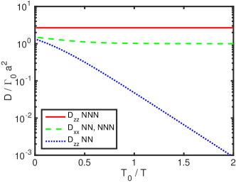
Figure 2: Predicted adatom diffusion coefficients $D_{xx}$ and $D_{zz}$ scaled by $\Gamma_{0}a^{2}$, vs. inverse temperature $T_{0}/T$ for the m-plane GaN surface. $D_{zz}$ depends upon the choice of NN or NNN diffusion model.

While we do not include an explicit ES step-edge barrier in our KMC model, as employed in other studies,Załuska-Kotur et al. (2012, 2011); Krzyżewski and Załuska-Kotur (2016) an effective barrier to diffusion down a step nevertheless arises because of the bonding geometry at the step. Detailed examination of the geometry of neighbors at different step edgesSup indicates that the NNN diffusion model produces a significantly smaller effective ES step-edge barrier, compared with the NN model. The effective ES barriers for the lowest-energy steps are summarized in Table 1 for the two diffusion models. Because we have suppressed diffusion to sites with $N_{i}=1$, as described below, the ES barrier is infinite for two cases in the NN model. (If jumps to $N=1$ sites had been allowed, the ES barriers would still have been large, $4E_{0}$ or $6E_{0}$, so their neglect has little effect on the growth simulation results.Sup ) In contrast, the NNN model has zero ES barrier in most cases (that is, no additional barrier above the standard barrier $E_{barr}$ for diffusion). For diffusion on the m-plane surface across a step normal to the $z$ direction, the NN model gives the same relatively high barrier of $4E_{0}$ at the step edge as for adatoms diffusing in the $z$ direction on the terrace. The NNN model reduces the ES barrier to $2E_{0}$. The NN and NNN models provide two extreme cases to demonstrate the effects of high and low ES barriers.

II.5 Implementation in SPPARKS

We carried out the KMC simulations on a 3-dimensional lattice using the Stochastic Parallel PARticle Kinetic Simulator (SPPARKS) computer code.Plimpton et al. (2009, ) The dynamics were calculated using the variable time step method known as the Gillespie or BKL algorithm.Gillespie (1977); Bortz et al. (1975) Details of the SPPARKS implementation are given in the supplemental material.Sup

Some exceptions to the general rules stated above are made to control unwanted behavior of the simulation. To suppress diffusion of atoms or dimers from the crystal surface into the volume of unoccupied sites above the crystal, the energy of atoms with $N_{i}=0$ or $1$ nearest neighbors is set to a large value. This has an additional effect of increasing the ES barrier for diffusion across certain step edges in the NN model, as described above.Sup To suppress diffusion of single vacancies in the bulk, the diffusion barrier for jumps from sites with $N_{i}=11$ to $N_{j}=11$ is set to a high value. If this is not done, at higher temperatures, vacancies from the surface will diffuse through the crystal and accumulate at the lower boundary of the simulation. Since no periodic boundary conditions are applied at the upper and lower boundaries of the simulation, the sites there have fewer neighboring sites and are thus energetically favorable for vacancies.

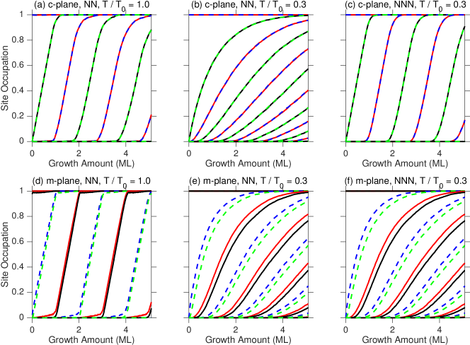
Figure 3: Fraction of sites occupied in each layer of unit cells during typical growth simulations. Growth rates were $G=5.3\times 10^{-6}$ or $5.0\times 10^{-6}$ ML/ut for c- or m-plane, respectively. Colors for sites 1-4 are red, black, blue and green respectively.

III Simulation Results

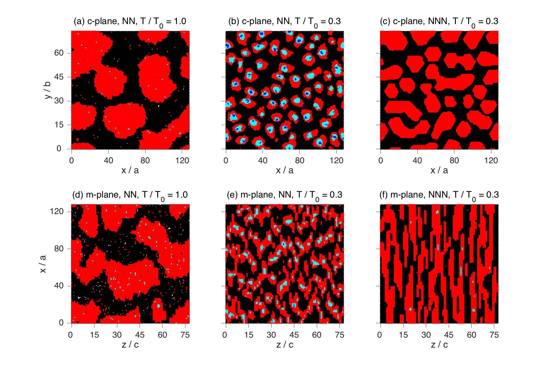
Figure 4: Surface islands after growth of 0.5 ML, for conditions of Fig. 3. The white, black, red, cyan, blue, and yellow colors represent the atoms at height of -1, 0, 1, 2, 3 and 4 ML above the initial surface.

III.1 Layer-by-layer and 3D growth modes

We investigated growth as a function of temperature $T$ and growth rate $G$, and observed the transition in the homoepitaxial growth modeTsao (1993) between layer-by-layer (LBL) and 3-dimensional (3D) for the c- and m-plane surfaces, using both NN and NNN diffusion models. Fig. 3 shows examples of the occupation fraction of each of the four sites in each layer of orthohexagonal unit cells shown in Fig. 1, as a function of time (plotted as growth amount).

On the c-plane, one can see that sites in the same monolayer fill at the same rate under all conditions. At high temperature, Fig. 3(a), growth occurs in LBL mode: each monolayer fills almost completely before there is significant occupation of the next monolayer. At low temperature in the NN model, Fig. 3(b), growth occurs in 3D mode: several layers fill simultaneously. At high temperature, the behavior of the NNN model (not shown) is very similar to that of the NN model. However, in the NNN model, LBL growth persists even at low temperature, Fig. 3(c).

On the m-plane, Figs. 3(d-f), all four sites fill at different rates. However, sites in the same monolayer, as defined above, begin to fill at about the same time and track fairly closely, especially at high temperature. The dependence of the growth mode on temperature and diffusion model is qualitatively similar to that seen on the c-plane; in the NN model, a transition from LBL to 3D growth is seen between $T=T_{0}$ and $T=0.3T_{0}$, while in the NNN model, LBL growth persists to lower temperature. The linearity of the occupancy curves in Fig. 3(d), with sharp changes in slope at the initiation or completion of each monolayer, indicates a nearly ideal LBL growth mode.Sup

III.1.1 Growth behavior in real space

Figure 4 shows the morphology of the islands on the surface after growth of 0.5 ML. The surface orientations, diffusion models, and conditions are the same as those for Fig. 3. As expected, the average island size and spacing is larger at higher $T$, Fig. 4 (a) and (d), than at lower $T$, reflecting the higher ratio of surface diffusion rate to growth rate. One can also see a significant population of adatoms and surface vacancies at higher $T$. For the NN diffusion model at $T$, Fig. 4 (b) and (e), multi-layer islands are forming even after only 0.5 ML of growth, indicating that atoms deposited onto islands experience a large effect of the ES step-edge barrier. However, the islands remain single-layer at lower $T$ for the NNN model, Fig. 4 (c) and (f), consistent with the lower ES barriers of the NNN diffusion model given in Table 1. There is little difference between NN and NNN (not shown) at higher $T$ for both c- and m-plane, because any ES barrier is easier to overcome. While islands on the c-plane surface are equiaxed at all temperatures, those on the m-plane surface become elongated in the $x$ direction at lower $T$ for the NNN model. For both c-plane and m-plane with the NNN model, the island edges become faceted at lower $T$, reflecting the low-energy step edge directions given in Table 1.

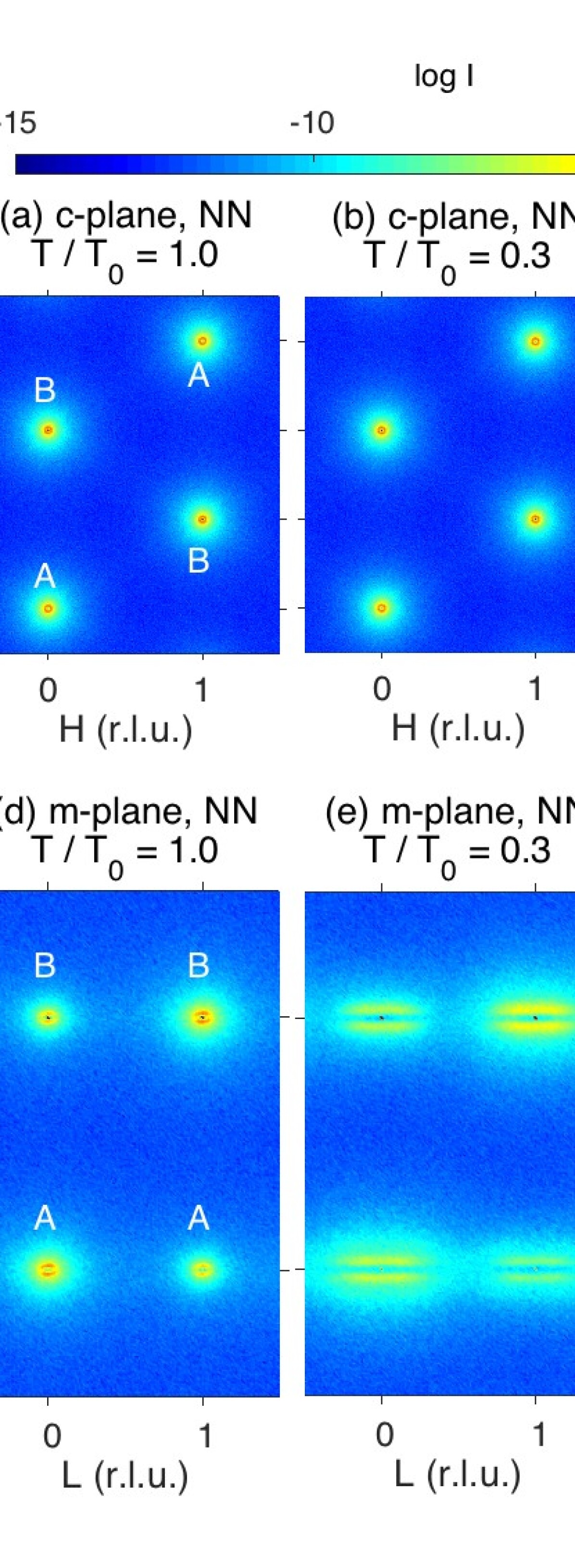
Figure 5: Reciprocal space intensity distributions after growth of $1/2$ ML, for conditions of Fig. 3. For the c-plane surfaces (a) - (c), the distribution in the $HK$ plane is shown at $L=1$. For the m-plane surfaces (d) - (f), the distribution in the $LH$ plane is shown at $K=1$. The color scale represents the logarithm of the intensity. Labels B and A indicate Bragg and anti-Bragg peaks.

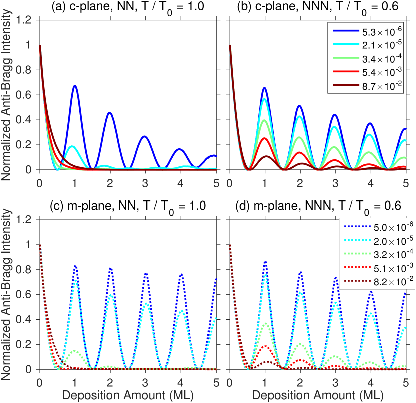
Figure 6: Anti-Bragg intensity at $(001)$ for c-plane and at $(010)$ for m-plane as a function of growth amount for growth rates shown in ML/ut, at fixed $T/T_{0}=1.0$ for NN kinetics and $T/T_{0}=0.6$ for NNN kinetics. Intensities are normalized to their initial values.

III.1.2 Reciprocal space

To quantitatively analyze the growth modes and island spacings, and to compare the results with surface X-ray scattering experiments, it is useful to calculate the intensity distribution in reciprocal space $I(H,K,L)$ (the square of the amplitude of the Fourier transform of the real space structure). Here we use reciprocal space coordinates $HKL$ of the orthohexagonal unit cells.Otte and Crocker (1965) Details are given in the Supplemental Material.Sup

The scattered intensity is proportional to the square of the complex structure factor $F$, which we calculate as the sum of terms from the simulation volume and from a semi-infinite crystal substrate located beneath the simulation volume.

$$I(H,K,L)\propto\left|F_{sim}+F_{sub}\right|^{2}$$ (5)

The substrate only contributes along the crystal truncation rods (CTRs)Fuoss and Brennan (1990) extending normal to the surface through the Bragg peaks at integer values of the in-plane reciprocal space coordinates ($H$ and $K$ for c-plane, $L$ and $H$ for m-plane).

The intensity distributions corresponding to typical 0.5 ML structures of Fig. 4 are shown in Fig. 5. While results in Figs. 3 and 4 are for single simulations, results in Fig. 5 and subsequent figures are obtained by averaging 16 simulations run with the same conditions but using different random number seeds. For the c-plane surfaces, Fig. 5(a-c), a slice through reciprocal space in the $HK$ plane at $L=1$ is shown. Peaks appear where CTRs running in the $L$ direction cut through the plane shown. Labels show Bragg peak positions from the bulk crystal lattice, and “anti-Bragg” positions half-way between Bragg peaks along the CTRs. For m-plane surfaces, Fig. 5(d-f), a slice through reciprocal space in the $LH$ plane at $K=1$ is shown.

Diffuse scattering intensity around the CTR positions reflects the in-plane structure of the crystal surface. For c-plane, the distribution of equiaxed islands with correlated positions gives rings of intensity in reciprocal space. The radius of the ring is inversely proportional to the spacing of the islands. When the island edges become faceted at lower $T$, the intensity distribution in reciprocal space shows streaks normal to the facets. For m-plane, the increasing anisotropy at lower $T$ gives very different distributions in the $H$ and $L$ directions. For the NN model, there are well-defined satellite peaks split in the $H$ direction, while for the NNN model the satellites are split in the $L$ direction. The satellites split along $H$ indicate a well-defined island spacing along $x$, while satellites split along $L$ indicate a well-defined island spacing along $z$. The amount of splitting is inversely proportional to the island spacing.

III.1.3 Evolution of anti-Bragg intensity

Alternate monolayers scatter exactly out of phase at anti-Bragg positions, giving good sensitivity to surface morphology from islands. Fig. 6 shows the average intensity at the anti-Bragg position in reciprocal space ($HKL=001$ for c-plane, $010$ for m-plane) as a function of growth amount at the different growth rates given in the legends, for each surface orientation and diffusion model. For the NN or NNN models, temperatures $T/T_{0}=1.0$ or $0.6$ are shown, respectively. For all cases, we see oscillations in intensity that reflect the growth mode. For ideal LBL growth, in which each monolayer completely coalesces before islands of the next monolayer form, the anti-Bragg intensity will make parabolic oscillations with equal maxima at integer monolayer amounts of deposition, and zero intensity at half-integer monolayer amounts. As the growth deviates from LBL and becomes 3D, new layers begin to form before the growth of the previous layer finishes, and the amplitude of the oscillation decreases and eventually disappears. In all cases in Fig. 6, we see this decrease in oscillation amplitude as growth rate increases, indicating the transition from LBL to 3D growth mode. We note that the positions of the maxima also shift away from integer monolayer amounts of deposition in the transition to 3D growth, and that the shift is to lower amounts for the NN model and to higher amounts for the NNN model. This reflects a change in the nature of the multilayer height distribution as the ES barrier is varied.

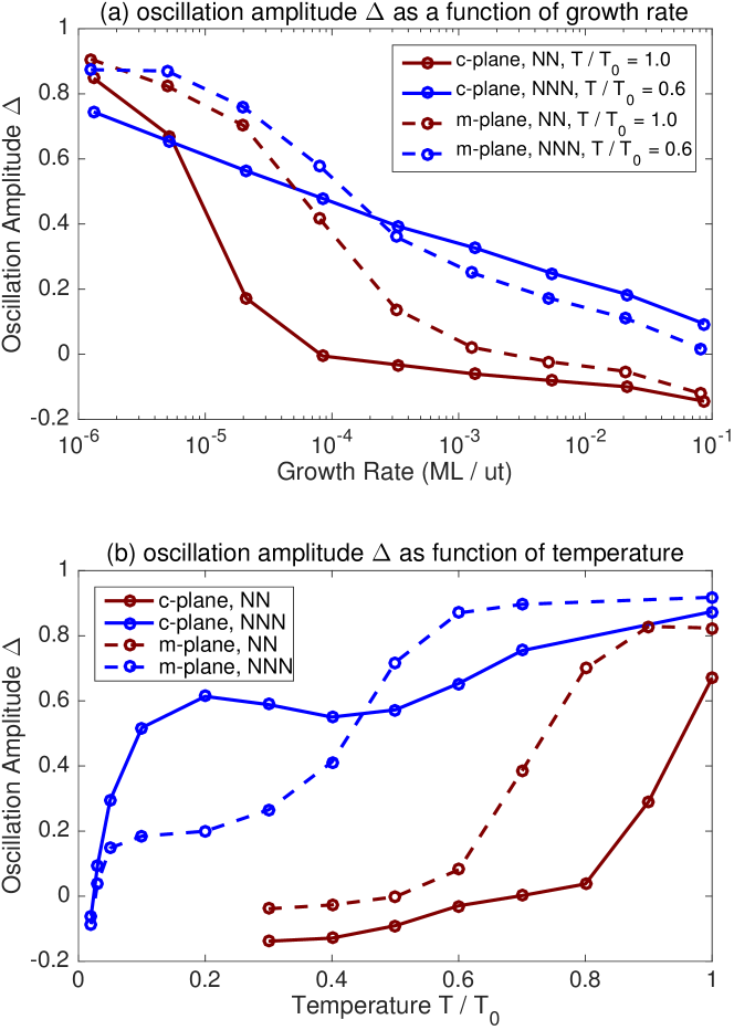
Figure 7: Comparison of oscillation amplitude $\Delta\equiv(I_{1}-I_{1/2})/I_{0}$ for c-plane and m-plane with NN and NNN kinetics. (a) $\Delta$ as a function of growth rate $G$ at fixed $T/T_{0}=1.0$ or $0.6$ for NN or NNN, respectively. (b) $\Delta$ as a function of $T/T_{0}$ at fixed $G=5.3$ or $5.0\times 10^{-6}$ ML/ut for c-plane or m-plane, respectively.

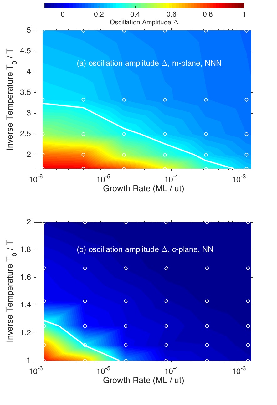
Figure 8: Plots of oscillation amplitude $\Delta$ as a function of inverse temperature and growth rate for (a) m-plane with NNN kinetics and (b) c-plane with NN kinetics. White circles show the conditions for the simulation data points, and the color scale gives the interpolated value of $\Delta$. The white contour at $\Delta=0.3$ indicates the LBL-3D growth mode boundary in each case. Note that $T_{0}/T$ range shown differs in (a) and (b).

III.1.4 Growth mode transition between LBL and 3D

To characterize the transition between LBL and 3D growth, we define a normalized oscillation amplitude $\Delta\equiv(I_{1}-I_{1/2})/I_{0}$, where $I_{1}$, $I_{1/2}$, and $I_{0}$ are the anti-Bragg intensity for growth amounts of $1$, $1/2$ and $0$ ML, respectively.Stephenson et al. (1999); Perret et al. (2014) Values of $\Delta$ approaching unity indicate perfect LBL growth, while values approaching zero (or becoming negative) indicate 3D growth. Here we choose a value of $\Delta=0.3$ to define the boundary between LBL and 3D growth.

Figure 7(a) shows the $\Delta$ values as a function of growth rate $G$ for c-plane (solid curves) and m-plane (dashed curves) with the NN model at a reduced temperature $T/T_{0}=1.0$ (red curves) or the NNN model at $T/T_{0}=0.6$ (blue curves). In all cases $\Delta$ decreases as growth rate increases, indicating a transition from LBL to 3D growth. Fig. 7(b) shows the $\Delta$ values as a function of temperature at fixed growth rates $G$ in ML/ut. Again the transition from LBL to 3D is reflected in the decrease in $\Delta$ as temperature decreases. For both m-plane and c-plane, the transition occurs at a lower $T$ with NNN kinetics compared with NN kinetics. The change is especially large for c-plane, compared with m-plane. For the NNN model on m-plane, the transition as a function of $T$ appears to occur in two steps, with some drop in $\Delta$ at intermediate $T$, followed by a sharp drop at low temperature, $T/T_{0}<0.1$. For the NNN model on c-plane, the primary drop occurs at low $T$. This behavior reflects two different mechanisms for the transition to 3D growth: adatoms become trapped on top of islands because of an ES step-edge barrier, or adatoms have insufficient time for surface diffusion compared with incoming deposition. The 3D growth mode will occur in all cases at low $T$ due the second mechanism. A transition to 3D can occur at intermediate $T$ due to the first mechanism, depending upon the magnitude of the ES barrier. For m-plane, where the NNN model reduces but does not eliminate the ES barrier for the dominant steps normal to the $z$ direction, we see the first mechanism is shifted to lower $T$ but not eliminated. For c-plane, the elimination of the ES barrier leaves only the second mechanism.

Figure 8 shows the behavior of $\Delta$ as a function of both growth rate and inverse temperature, for m-plane with NNN kinetics and c-plane with NN kinetics. (We focus on these two cases because they agree best with experiments, as described below. Results for the m-plane with NN kinetics were also obtained, and are shown in the supplemental material.Sup ) Contours of constant $\Delta$ on this plot are reasonably straight lines, indicating that the temperature dependence of the growth rate at the LBL-to-3D boundary $G_{3D}$ can be described by the Arrhenius expression

$$G_{3D}=A_{3D}\exp(-E_{3D}/kT).$$ (6)

For each temperature, we interpolated between the $\Delta$ values to determine the boundary growth rate $G_{3D}$ giving $\Delta=0.3$, and fit these values with Eq. 6. Parameters obtained from these fits are given in Table 2.

Table 2: Parameters of Eq. 6 obtained from fits to the growth rate as a function of temperature at the LBL-3D boundary defined by $\Delta=0.3$.

Surface	Diffusion	$E_{3D}/E_{0}$	$\log_{10}A_{3D}$
Orient.	Model		(ML/ut)
c-plane	NN	$8.41\pm 0.57$	$-1.20\pm 0.28$
m-plane	NNN	$3.81\pm 0.09$	$-0.42\pm 0.08$

III.2 Island spacing and step-flow growth

III.2.1 Diffuse scattering

Characteristics of the island structure on the crystal surface can be obtained by analyzing the in-plane diffuse scattering around the CTRs at 0.5 ML of growth, such as that shown in Fig. 5.

For the m-plane surface, the diffuse scattering is not isotropic. We see symmetric satellite peaks on both sides of the CTR, displaced in the in-plane directions $L$ or $H$ for the NNN or NN results, respectively. For the NNN model, we analyzed the intensity distribution averaged over $H$ within a region centered on the CTR. Fig. 9(a) shows typical plots of the diffuse intensity as a function of $Q_{L}$ around the $(010)$ CTR on the m-plane surface with NNN kinetics, for various growth rates at $T/T_{0}=0.6$. We extracted the positions by self-consistently calculating the center of mass $\overline{Q}$ of the intensity distribution for $Q_{L}>0$ within the range from $0.4\,\overline{Q}$ to $1.6\,\overline{Q}$ using an iterative procedure. The extracted value of $\overline{Q}$ for each curve on Fig. 9 is shown by the square symbol.

For the c-plane surface, a nearly isotropic ring of intense diffuse scattering indicates an isotropic arrangement of islands with correlated spacings. To characterize these rings, we performed an azimuthal average centered on the CTR position to obtain the intensity as a function of reciprocal space radius $Q$ (in units of $2\pi/a$). Fig. 9(b) shows typical plots of the diffuse intensity around the $(001)$ CTR on the c-plane surface with NN kinetics, for various growth rates at $T/T_{0}=1.0$. As for the m-plane, we see peaked intensity distributions, the positions of which are inversely related to the average island spacings.

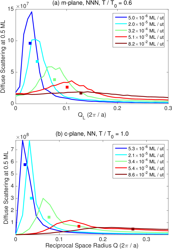
Figure 9: Diffuse scattering profiles near the CTR at 0.5 ML for different growth rates given in legend. (a) m-plane, $T/T_{0}=0.6$, NNN kinetics; (b) c-plane, $T/T_{0}=1.0$, NN kinetics. Square symbols show the extracted positions $\overline{Q}$.

III.2.2 Island spacing

The average island spacing in real space $S$ can be obtained from the peak position in reciprocal space using $S=2\pi/\overline{Q}$. Fig. 10 shows the island spacing at 0.5 ML as a function of growth rate and inverse temperature for m-plane with NNN kinetics and c-plane with NN kinetics.

In the LBL region, the temperature and growth rate dependence of the island spacing can be modeled using an expression from nucleation theory,Evans and Bartelt (1994)

$$S/a=(G/G_{S})^{-n}\exp(-nE_{S}/kT),$$ (7)

where island spacing $S$ has been scaled by the $a$ lattice parameter. We have fit the island spacings for higher temperatures and lower growth rates to this expression, as shown in Fig. 11, and obtained the fit parameters, $n$, $E_{s}$ and $G_{s}$, given in Table 3.

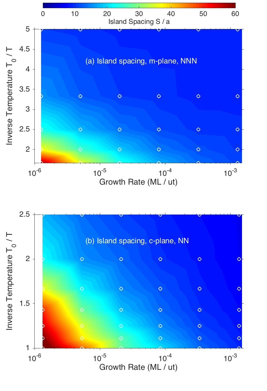
Figure 10: Island spacing $S/a$ at 0.5 ML as a function of inverse temperature and growth rate for (a) m-plane with NNN kinetics and (b) c-plane with NN kinetics. The white circles show the conditions for the simulation data points, and the color scale gives the interpolated value of $S/a$. Note that the $T_{0}/T$ range shown differs in (a) and (b).

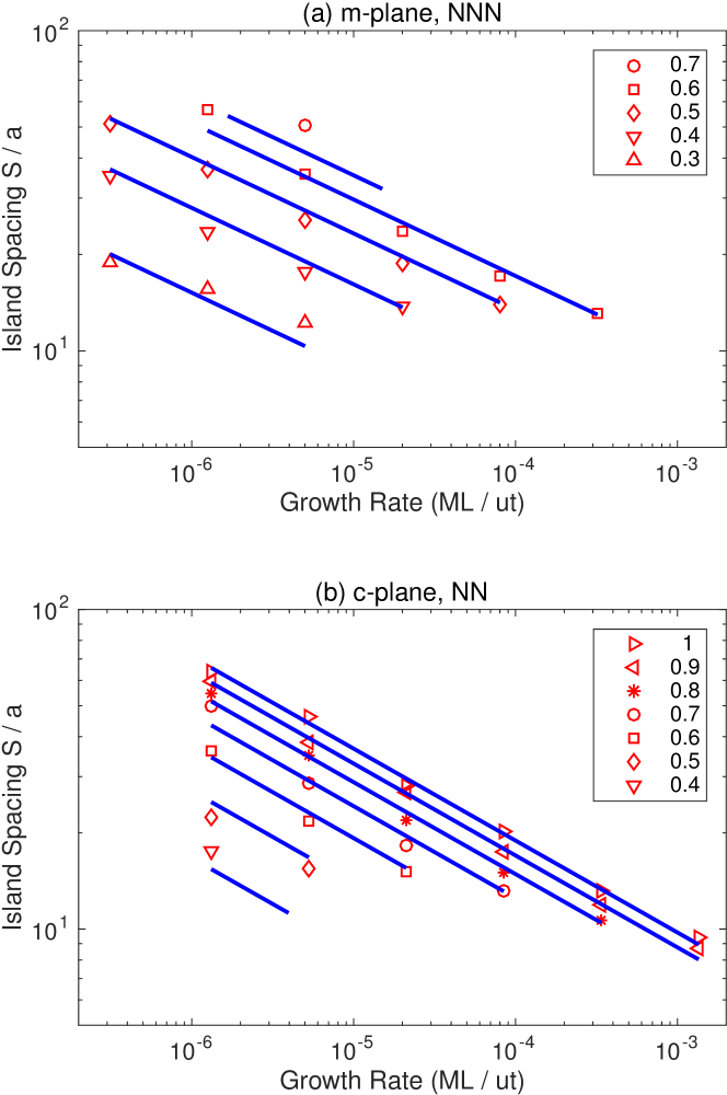
Figure 11: Island spacing $S/a$ at 0.5 ML as a function of growth rate at various $T/T_{0}$ given in legend, for (a) m-plane with NNN kinetics and (b) c-plane with NN kinetics. Lines are fit of all points in each plot to Eq. 7.

Table 3: Parameters of Eq. 7 obtained from fits to island spacings.

Surface	Diffusion	$n$	$E_{S}/E_{0}$	$\log_{10}G_{S}$
Orient.	Model			(ML/ut)
c-plane	NN	$0.288\pm 0.007$	$3.36\pm 0.13$	$1.90\pm 0.10$
m-plane	NNN	$0.239\pm 0.014$	$3.06\pm 0.19$	$3.39\pm 0.29$

III.2.3 Step-flow transition

In this study we consider surfaces oriented exactly on the crystallographic c- or m-planes. On vicinal surfaces away from these exact orientations, long-range step arrays are present and growth can occur by the step-flow (SF) mode, in which adatoms attach to the step arrays in preference to nucleating islands. The boundary between SF and LBL growth modes is expected to occur when the island nucleation spacing $S$ equals the terrace width (step spacing) $W$ of the vicinal surface.Tsao (1993) While we do not directly model vicinal surfaces in this study, an expression for the boundary can be obtained by substituting $S=W$ into Eq. 7 and solving for the growth rate as a function of $T$ and $W$,

$$G_{SF}=G_{S}\,(W/a)^{-1/n}\exp(-E_{S}/kT).$$ (8)

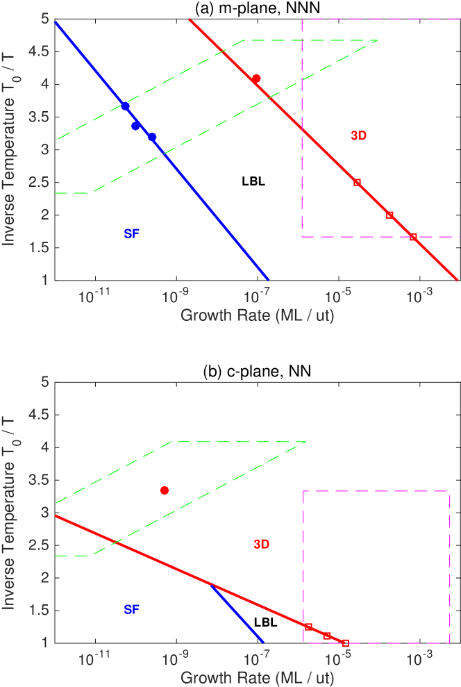
Figure 12: Predicted homoepitaxial growth mode transitions on GaN surfaces, for (a) m-plane with NNN kinetics and (b) c-plane with NN kinetics. Red and blue lines show the boundaries between 3-dimensional (3D), layer-by-layer (LBL) and step-flow (SF) growth modes, for a terrace width $W/a=125$. Magenta and green dashed boundaries show ranges of conditions for simulations and experiments, respectively.

Figure 12 shows the predicted growth mode boundaries for the m-plane surface with NNN kinetics, and the c-plane surface with NN kinetics, as a function of growth rate $G$ and inverse temperature. The LBL-3D boundaries are obtained from the fits of the simulation values of $G_{3D}$ using Eq. 6 given in Table 2. The SF-LBL boundaries are from Eq. 8 using the values in Table 3 and $W/a=125$, which corresponds to the experimental results.Perret et al. (2014) Note that these boundaries are extrapolated outside of the region directly investigated in the simulations. The range of LBL growth is much wider for the m-plane than for the c-plane, primarily because the large ES barrier for the c-plane with NN kinetics expands the 3D growth region.

IV Comparison with Experiment

IV.1 Length, energy, temperature, and time units for GaN MOVPE

To compare the KMC results quantitatively with experiment, we can relate the dimensionless units of the simulations to units appropriate for GaN growth by MOVPE. The length scale for GaN is given simply by its crystal lattice parameters, which are $a=0.32$ nm and $c=0.52$ nm at 1000 K.Moram and Vickers (2009)

To estimate the energy scale for GaN, the total energy per lattice site, $12E_{0}$, can be equated to the enthalpy of formation of solid GaN from vapor GaN, $\Delta H_{f}^{solid}-\Delta H_{f}^{vapor}=-3.38$ eV per moleculePrzhevalskii et al. (1998) at 1000 K. This gives an energy unit for the simulation of $E_{0}=0.282$ eV, and a characteristic temperature of $T_{0}=3275$ K. Thus typical GaN MOVPE growth temperatures of 1000 to 1600 K correspond to simulation conditions in the range $T/T_{0}=0.3$ to $0.5$.

The time unit $t_{0}$ (s/ut) is a temperature dependent quantity that depends on the $\nu_{0}$ and $E_{barr}$ values that enter into the surface diffusion coefficients, e.g. $D=\frac{3}{2}a^{2}\nu_{0}\exp(-E_{barr}/kT)$ for the c-plane surface. An expression for $t_{0}$ can be obtained by taking the ratio of $\Gamma_{0}$ in simulation units (ut^-1) and in experimental units (s^-1),

$$t_{0}=\frac{\exp(-0.3T_{0}/T)}{\nu_{0}\exp(-E_{barr}/kT)}.$$ (9)

Note that the time unit $t_{0}(T)$ is a function of temperature. Thus the growth rate $G/t_{0}$ in ML/s (experiment units) changes with temperature at fixed growth rate $G$ in ML/ut (simulation units). Values for $t_{0}$ are estimated below based on the observed SF-LBL growth mode boundary for m-plane GaN MOVPE.

IV.2 Island height and shape

The heights of the islands observed during LBL growth in the simulations (e.g. Figs. 3 and 4) were $c/2$ for the c-plane and $b/2$ for the m-plane, which we defined to be 1 ML in each case. These heights agree with those observed in experiments for both c-planeStephenson et al. (1999); Thompson et al. (2001); Munkholm et al. (2000) and m-plane.Perret et al. (2014)

The arrangement and anisotropy of the island shapes for m-plane seen in the simulations differ significantly between the NN and NNN kinetic models at lower $T$, as shown in Figs. 4(e) and (f). In particular, the NNN model gives islands that are elongated in the $x$ direction and have a well-defined spacing in the $z$ direction. This is in agreement with experimental observations of island shapes on m-plane surfaces, as shown in Fig. 13.

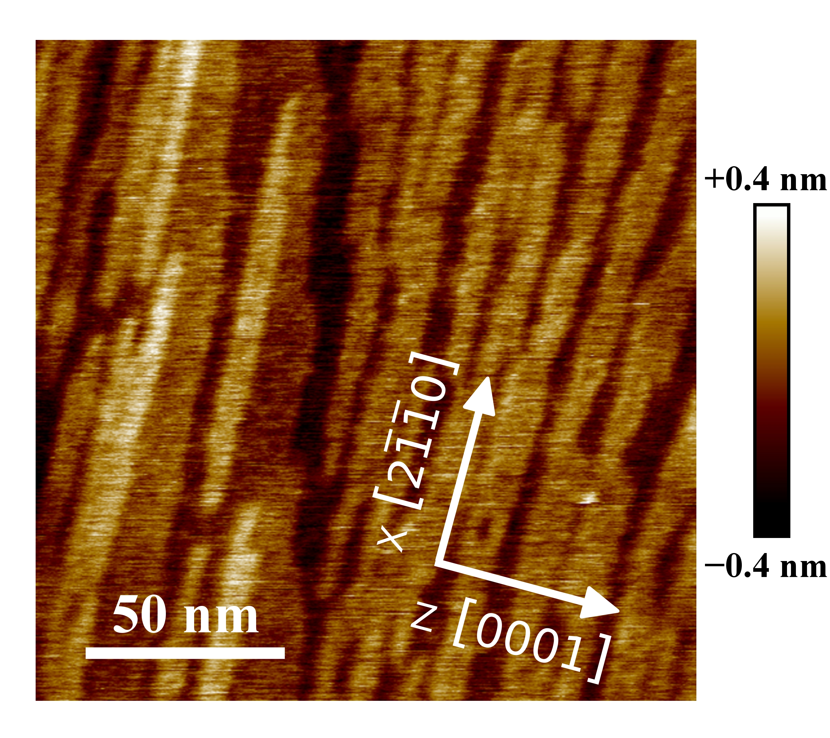
Figure 13: Atomic force microscopy (AFM) topography image of m-plane surface with 0.5 ML coverage of islands grown under LBL conditions.Perret et al. (2014, 2016). Islands are elongated normal to $z$, as in Fig. 4(f) for the NNN model.

Table 4: Reduced temperature and time units, and calculated adatom diffusion coefficients for c- amd m-plane surfaces, as a function of actual temperature, using estimated parameters for GaN MOVPE: $T_{0}=3275$ K, $E_{barr}=2.05$ eV, and $\nu_{0}=3\times 10^{18}$ s^-1. Values of $D_{zz}$ for m-plane use the NNN model.

$T$	$T/T_{0}$	$t_{0}$	$D$ (c)	$D_{xx}$ (m)	$D_{zz}$ (m)
(K)		(s)	(cm2/s)	(cm2/s)	(cm2/s)
1000	0.31	$2.5\times 10^{-9}$	$2.3\times 10^{-7}$	$1.5\times 10^{-7}$	$4.0\times 10^{-7}$
1250	0.38	$2.6\times 10^{-11}$	$2.6\times 10^{-5}$	$1.8\times 10^{-5}$	$4.7\times 10^{-5}$
1500	0.46	$1.3\times 10^{-12}$	$6.3\times 10^{-4}$	$4.2\times 10^{-4}$	$1.1\times 10^{-3}$

IV.3 Growth mode boundaries

As shown in Fig. 12, the simulations predict a much larger region of LBL growth for m-plane than c-plane surfaces. This result is consistent with experiments,Thompson et al. (2001); Perret et al. (2014) in which a direct transition between SF and 3D growth modes is typically observed on c-plane, while a large intervening region of LBL growth is observed on m-plane.

The observed growth rate at the SF-LBL boundary on m-plane GaNPerret et al. (2014) can be described by an Arrhenius expression

$$G_{SF}^{obs}=A_{SF}^{obs}\exp(-E_{SF}^{obs}/kT),$$ (10)

with parameters $E_{SF}^{obs}=2.83\pm 0.27$ eV and $\log_{10}[A_{SF}^{obs}$ (ML/s)$]=13.1\pm 1.4$. By equating $G_{SF}^{obs}$ in ML/s with $G_{SF}/t_{0}$ from Eqs. 8 and 9, we can obtain expressions for the parameters that give the time scale for GaN MOVPE,

$$E_{barr}=E_{SF}^{obs}-E_{S}+0.3E_{0}.$$ (11)

$$\log(\nu_{0})=\log(A_{SF}^{obs})-\log(G_{S})+n^{-1}\log(W/a),$$ (12)

Using the terrace width $W=40\pm 10$ nm corresponding to the experimentsPerret et al. (2014) and the simulation value of $n=0.239\pm 0.014$, this gives $E_{barr}=2.05\pm 0.28$ eV and $\log_{10}[\nu_{0}$ (s${}^{-1})]=18.5\pm 1.8$. Values of $t_{0}$ estimated using these parameters are given in Table 4. Also shown are the calculated surface diffusion coefficients.Sup

Using the correspondence between experimental and simulation temperature and time scales given in Table 4, the regions of temperature and growth rate investigated in recent experimentsPerret et al. (2014) are shown in Fig. 12. The boundaries at fixed experimental growth rates of 0.001 and 2 ML/s appear as diagonal lines when plotted in simulation units of ML/ut, because of the temperature dependence of $t_{0}$. Except at low temperature, the region investigated directly in the current simulations corresponds to much higher growth rates than studied in experiments. The three experimental values of $G_{SF}^{obs}$ used to obtain the correspondence are likewise plotted in simulation units (blue dots) on Fig. 12(a).

The experimentally observed value of $G_{3D}$ at the LBL-3D transition for m-planePerret et al. (2014) is plotted (red dot) in simulation units on Fig. 12(a). It lies very close to the boundary obtained from the simulation results (red line). This represents a quantitative agreement of the relative positions of the SF-LBL and LBL-3D boundaries between the experiments and the simulations using the NNN model for the m-plane surface.

Experiments on c-plane surfacesPerret et al. (2014) show a direct transition between SF and 3D growth modes, with no intervening LBL mode. This qualitatively agrees with the prediction in Fig. 12(b) for the region of experimental conditions. However, the experimentally observed value for $G_{3D}$ (red dot) is significantly higher than the boundary predicted by simulations using the NN model for the c-plane surface (red line). This quantitative difference may indicate that the effective ES barriers produced by the NN model are too large to accurately represent the c-plane, and that behavior intermediate between those of the NN and NNN simulations would agree better with experiment. However, because we have used results from m-plane to determine the correspondence between experimental and simulation time scales, other effects may also contribute to the difference observed for c-plane.

V Discussion and Conclusions

The simulations presented here of growth on the c- and m-plane surfaces of a hexagonal crystal provide both agreement with, and insight into, experimental results for MOVPE growth of GaN. We see different behavior on the two surfaces because of the different bonding configurations. The simulations employ two different models for diffusion kinetics: NN, which allows diffusion jumps only between nearest-neighbor sites; and NNN, which also allows some next-nearest-neighbor jumps. These produce higher and lower effective Ehrlich-Schwoebel step-edge barriers, respectively, and have a significant impact on the crystal growth modes. We have mapped the transitions as a function of temperature $T$ and growth rate $G$ among the three homoepitaxial growth modes: three-dimensional (3D); layer-by-layer (LBL); and step-flow (SF). We have also determined the dependence on $T$ and $G$ of the island spacing $S$ that develops during LBL and 3D growth. Quantitative comparison of these results to experiment allows us to estimate underlying fundamental quantities, such as the surface diffusion coefficients given in Table 4.

On both the c- and m-plane surfaces, the island heights found in the simulations during LBL growth are one half of the orthohexagonal unit cell dimension ($c/2$ and $b/2$, respectively). This is in agreement with experimental studies of layer-by-layer growth in GaN MOVPE,Stephenson et al. (1999); Thompson et al. (2001); Munkholm et al. (2000); Perret et al. (2014) indicating that the basic nearest-neighbor bond counting energetics of the KMC model is generally applicable to this system. The simulations show that both the typical island shapes at lower temperatures and the growth mode transitions differ between c- and m-plane, and between NN and NNN kinetics. Overall, the NN model with high ES barrier provides better agreement with experiment for the c-plane, while the NNN model with low ES barrier provides better agreement for m-plane. In particular, the very narrow region of LBL growth found for c-plane with NN kinetics, and the typical shape of islands on m-plane formed under NNN kinetics (elongated perpendicular to $[0001]$ and highly correlated parallel to $[0001]$), are both in agreement with X-rayPerret et al. (2014) and AFM measurements. This indicates that the elongated islands observed on m-plane have their origin primarily in anisotropic equilibrium step-edge energies rather than in adatom diffusion kinetics, since the latter is almost isotropic in the NNN model. Similar conclusions were reached in studies of islands on dimerized Si (001) Clarke et al. (1991) and Ag (110) Ferrando et al. (1997).

Our study indicates that the direct transition from SF to 3D growth observed for growth on GaN c-plane surfaces can be attributed to a high ES barrier due to the bonding arrangement at steps on a close-packed surface. Previous KMC studies on c-plane growth also emphasized the effect of the ES barrier on island nucleation, finding that smoother films are obtained when the ES barrier is screened.Kaufmann et al. (2016) This agrees with our finding that the LBL range is wider on c-plane when using the NNN model.

Our simulations found that the island spacing $S$ under LBL growth conditions obeys a negative power-law dependence on growth rate, Eq. 7, with exponent $n=0.24$ for m-plane and $n=0.29$ for c-plane. Recent experimental results Perret et al. (2016) for MOVPE on m-plane GaN are in agreement with this value. Growth of anisotropic islands in submonolayer epitaxy has been previously considered in KMC modeling. Heyn (2001); Clarke et al. (1991); Evans et al. (2006) The power law for island density as a function of growth rate shows an exponent smaller than that for the isotropic case, with $n=1/4$ for a critical nucleus size equal to one. However, we observe a similar low exponent in our simulations on c-plane surfaces, where the island shapes are isotropic.

Several topics for future work can be identified. There is considerable interest in GaN growth on surface orientations in addition to c- and m-plane,Kelchner et al. (2015) and it is straightforward to extend the KMC model and methods developed here to other orientations. While we have estimated the boundary between LBL and SF growth based on island spacing, it will be of interest to explicitly consider growth on vicinal surfaces with steps, which can be done by using helical boundary conditions.Krzyżewski et al. (2016) For simplicity we have neglected evaporation from the surface in this work. Inclusion of evaporation will provide a second surface transport mechanism qualitatively different from surface diffusion, that undoubtedly becomes important at higher temperatures.Mitchell et al. (2001) Since the KMC model gives an exact arrangement as a function of time for the atomic positions, it will be very valuable in predicting the results of coherent X-ray experiments (such as X-ray photon correlation spectroscopy Shpyrko (2014) or coherent diffraction imaging Abbey (2013)) that are becoming feasible. The model also can be extended to account for full the wurtzite structure of GaN, with two atom types and additional parameters derived from experiment or ab initio theory. This will allow study of the effects of polarity. Finally, the NN and NNN models employed here give fairly extreme values for high and low effective ES barriers. The best agreement with experiments may be obtained from a model between these two extremes.

VI Acknowledgements

We gratefully acknowledge support provided by the Department of Energy, Office of Science, Basic Energy Sciences, Scientific User Facilities (KMC model development) and Materials Sciences and Engineering (reciprocal space analysis and experiments), and computing resources provided on Blues and Fusion, high-performance computing clusters operated by the Laboratory Computing Resource Center at Argonne National Laboratory.

See pages 1 of 2016_Xu_KMC_GaN_nosteps_SUPPLEMENTAL_PRB.pdf See pages 2 of 2016_Xu_KMC_GaN_nosteps_SUPPLEMENTAL_PRB.pdf See pages 3 of 2016_Xu_KMC_GaN_nosteps_SUPPLEMENTAL_PRB.pdf See pages 4 of 2016_Xu_KMC_GaN_nosteps_SUPPLEMENTAL_PRB.pdf See pages 5 of 2016_Xu_KMC_GaN_nosteps_SUPPLEMENTAL_PRB.pdf See pages 6 of 2016_Xu_KMC_GaN_nosteps_SUPPLEMENTAL_PRB.pdf See pages 7 of 2016_Xu_KMC_GaN_nosteps_SUPPLEMENTAL_PRB.pdf See pages 8 of 2016_Xu_KMC_GaN_nosteps_SUPPLEMENTAL_PRB.pdf See pages 9 of 2016_Xu_KMC_GaN_nosteps_SUPPLEMENTAL_PRB.pdf See pages 10 of 2016_Xu_KMC_GaN_nosteps_SUPPLEMENTAL_PRB.pdf See pages 11 of 2016_Xu_KMC_GaN_nosteps_SUPPLEMENTAL_PRB.pdf See pages 12 of 2016_Xu_KMC_GaN_nosteps_SUPPLEMENTAL_PRB.pdf See pages 13 of 2016_Xu_KMC_GaN_nosteps_SUPPLEMENTAL_PRB.pdf See pages 14 of 2016_Xu_KMC_GaN_nosteps_SUPPLEMENTAL_PRB.pdf See pages 15 of 2016_Xu_KMC_GaN_nosteps_SUPPLEMENTAL_PRB.pdf See pages 16 of 2016_Xu_KMC_GaN_nosteps_SUPPLEMENTAL_PRB.pdf

References

- Nanishi (2014) Y. Nanishi, Nature Photonics 8, 884 (2014).
- Nie et al. (2014) H. Nie, Q. Diduck, B. Alvarez, A. P. Edwards, B. M. Kayes, M. Zhang, G. Ye, T. Prunty, D. Bour, and I. C. Kizilyalli, IEEE Electron Device Letters 35, 939 (2014).
- DenBaars et al. (2013) S. P. DenBaars, D. Feezell, K. Kelchner, S. Pimputkar, C.-C. Pan, C.-C. Yen, S. Tanaka, Y. Zhao, N. Pfaff, R. Farrell, M. Iza, S. Keller, U. Mishra, J. S. Speck, and S. Nakamura, Acta Materialia 61, 945 (2013).
- Waltereit et al. (2000) P. Waltereit, O. Brandt, A. Trampert, H. Grahn, J. Menniger, M. Ramsteiner, M. Reiche, and K. Ploog, Nature 406, 865 (2000).
- Nakamura and Krames (2013) S. Nakamura and M. Krames, Proceedings of the IEEE 101, 2211 (2013).
- Fujita (2015) S. Fujita, Japanese Journal of Applied Physics 54, 030101 (2015).
- Chugh and Ranganathan (2015) M. Chugh and M. Ranganathan, physica status solidi (c) 12, 408 (2015).
- Wang et al. (1994) K. Wang, J. Singh, and D. Pavlidis, Journal of Applied Physics 76, 3502 (1994).
- Fu et al. (2008) K. Fu, Y. Fu, P. Han, Y. Zhang, and R. Zhang, Journal of Applied Physics 103, 103524 (2008).
- Załuska-Kotur et al. (2012) M. A. Załuska-Kotur, F. Krzyżewski, and S. Krukowski, Journal of Crystal Growth 343, 138 (2012).
- Załuska-Kotur et al. (2011) M. A. Załuska-Kotur, F. Krzyżewski, and S. Krukowski, Journal of Applied Physics 109, 023515 (2011).
- Załuska-Kotur et al. (2010) M. A. Załuska-Kotur, F. Krzyżewski, and S. Krukowski, Journal of Non-Crystalline Solids 356, 1935 (2010).
- Ehrlich and Hudda (1966) G. Ehrlich and F. G. Hudda, The Journal of Chemical Physics 44, 1039 (1966).
- Schwoebel and Shipsey (1966) R. L. Schwoebel and E. J. Shipsey, Journal of Applied Physics 37, 3682 (1966).
- Kaufmann et al. (2016) N. A. Kaufmann, L. Lahourcade, B. Hourahine, D. Martin, and N. Grandjean, Journal of Crystal Growth 433, 36 (2016).
- Krzyżewski et al. (2016) F. Krzyżewski, M. A. Załuska-Kotur, H. Turski, M. Sawicka, and C. Skierbiszewski, Journal of Crystal Growth , (2016).
- Krzyżewski and Załuska-Kotur (2016) F. Krzyżewski and M. A. Załuska-Kotur, Journal of Crystal Growth , (2016).
- Stephenson et al. (1999) G. B. Stephenson, J. A. Eastman, C. Thompson, O. Auciello, L. J. Thompson, A. Munkholm, P. Fini, S. P. DenBaars, and J. S. Speck, Applied Physics Letters 74, 3326 (1999).
- Thompson et al. (2001) C. Thompson, G. B. Stephenson, J. A. Eastman, A. Munkholm, O. Auciello, M. V. R. Murty, P. Fini, S. P. DenBaars, and J. S. Speck, Journal of The Electrochemical Society 148, C390 (2001).
- Munkholm et al. (2000) A. Munkholm, C. Thompson, M. V. Ramana Murty, J. A. Eastman, O. Auciello, G. B. Stephenson, P. Fini, S. P. DenBaars, and J. S. Speck, Applied Physics Letters 77, 1626 (2000).
- Perret et al. (2014) E. Perret, M. J. Highland, G. B. Stephenson, S. K. Streiffer, P. Zapol, P. H. Fuoss, A. Munkholm, and C. Thompson, Applied Physics Letters 105, 051602 (2014).
- Koleske et al. (2014) D. D. Koleske, S. R. Lee, M. H. Crawford, K. C. Cross, M. E. Coltrin, and J. M. Kempisty, Journal of Crystal Growth 391, 85 (2014).
- Lymperakis and Neugebauer (2009) L. Lymperakis and J. Neugebauer, Phys. Rev. B 79, 241308 (2009).
- Krukowski et al. (2009) S. Krukowski, P. Kempisty, and P. Strąk, Cryst. Res. Technol. 44, 1038 (2009).
- Walkosz et al. (2012a) W. Walkosz, P. Zapol, and G. B. Stephenson, The Journal of Chemical Physics 137, 054708 (2012a).
- Walkosz et al. (2012b) W. Walkosz, P. Zapol, and G. B. Stephenson, Physical Review B 85, 033308 (2012b).
- An et al. (2015) Q. An, A. Jaramillo-Botero, W.-G. Liu, and I. William. A. Goddard, The Journal of Physical Chemistry C 119, 4095 (2015).
- Jindal and Shahedipour-Sandvik (2010) V. Jindal and F. Shahedipour-Sandvik, Journal of Applied Physics 107, 054907 (2010), 10.1063/1.3309840.
- Ambacher et al. (1996) O. Ambacher, M. S. Brandt, R. Dimitrov, T. Metzger, M. Stutzmann, R. A. Fischer, A. Miehr, A. Bergmaier, and G. Dollinger, Journal of Vacuum Science & Technology B 14, 3532 (1996).
- Moram and Vickers (2009) M. A. Moram and M. E. Vickers, Reports on Progress in Physics 72, 036502 (2009).
- Otte and Crocker (1965) H. M. Otte and A. G. Crocker, Physica Status Solidi (b) 9, 441 (1965).
- Xie et al. (1999) M. H. Xie, S. M. Seutter, W. K. Zhu, L. X. Zheng, H. Wu, and S. Y. Tong, Phys. Rev. Lett. 82, 2749 (1999).
- Giesen (2001) M. Giesen, Progress in Surface Science 68, 1 (2001).
- (34) See Supplemental Material at [URL will be inserted by publisher] for details of the assumptions used, and supplemental results of, the kinetic Monte Carlo (KMC) model developed for GaN homoepitaxy.
- Tsao (1993) J. Y. Tsao, Materials Fundamentals of Molecular Beam Epitaxy (Academic Press, Inc., San Diego, CA, 1993).
- Plimpton et al. (2009) S. Plimpton, C. Battaile, M. Chandross, L. Holm, A. Thompson, V. Tikare, G. Wagner, E. Webb, X. Zhou, C. G. Cardona, and A. Slepoy, Crossing the Mesoscale No-Man’s Land via Parallel Kinetic Monte Carlo, Tech. Rep. SAND2009–6226 (Sandia National Laboratories, 2009).
- (37) S. Plimpton, A. Thompson, and A. Slepoy, “SPPARKS kinetic Monte Carlo simulator (version 08 jul 2015),” Version 08 July 2015.
- Gillespie (1977) D. T. Gillespie, The journal of physical chemistry 81, 2340 (1977).
- Bortz et al. (1975) A. Bortz, M. Kalos, and J. Lebowitz, Journal of Computational Physics 17, 10 (1975).
- Fuoss and Brennan (1990) P. H. Fuoss and S. Brennan, Annual Review of Materials Science 20, 365 (1990).
- Evans and Bartelt (1994) J. W. Evans and M. C. Bartelt, Journal of Vacuum Science & Technology A 12, 1880 (1994).
- Przhevalskii et al. (1998) I. N. Przhevalskii, S. Y. Karpov, and Y. N. Makarov, MRS Internet Journal of Nitride Semiconductor Research 3 (1998).
- Perret et al. (2016) E. Perret, D. Xu, M. J. Highland, G. B. Stephenson, P. Zapol, P. H. Fuoss, A. Munkholm, and C. Thompson, (2016), unpublished.
- Clarke et al. (1991) S. Clarke, M. R. Wilby, and D. D. Vvedensky, Surface Science 255, 91 (1991).
- Ferrando et al. (1997) R. Ferrando, F. Hontinfinde, and A. C. Levi, Physical Review B Rapid Communications 56, R4406 (1997).
- Heyn (2001) C. Heyn, Phys. Rev. B 63, 033403 (2001).
- Evans et al. (2006) J. Evans, P. Thiel, and M. Bartelt, Surface Science Reports 61, 1 (2006).
- Kelchner et al. (2015) K. Kelchner, L. Kuritzky, S. Nakamura, S. DenBaars, and J. Speck, Journal of Crystal Growth 411, 56 (2015).
- Mitchell et al. (2001) C. C. Mitchell, M. E. Coltrin, and J. Han, Journal of Crystal Growth 222, 144 (2001).
- Shpyrko (2014) O. G. Shpyrko, Journal of Synchrotron Radiation 21, 1057 (2014).
- Abbey (2013) B. Abbey, JOM 65, 1183 (2013).