What is dimension?

 

This chapter explores the notion of “dimension” of a set. Various power laws by which an Euclidean space can be characterized are used to define dimensions, which then explore different aspects of the set. Also discussed are the generalization to multifractals, and discrete and continuous scale invariance with the emergence of complex dimensions. The idea of renormalization group flow equations can be introduced in this framework, to show how the power laws determined by dimensional analysis (engineering dimensions) get modified by extra anomalous dimensions. As an example of the RG flow equation, the scaling of conductance by disorder in the context of localization is used. A few technicalities, including the connection between entropy and fractal dimension, can be found in the appendices.

 

 

1 Introduction

The purpose of this chapter is to explore the idea of “dimension” of a set. E.g., what does superscript 1 mean when we talk of $S^{1}$? The vector space idea of the minimum number of basis vectors is too restrictive to be applicable to even many subsets of standard Euclidean manifolds, which are not necessarily vector spaces. Generalizations of the definition of dimension consistent with the intuitions based on Euclidean spaces give a large number of possibilities, with each one describing some aspect of the set. These dimensions need not be integers anymore. If various physical phenomena are studied on these subsets, which “dimension” will matter?

Once released from the integer constraint, there is no restriction on the value of dimension, with examples of positive, negative, real, and complex, $d$, even cases which require more than one $d$. Such varieties are not possible in ordinary Euclidean spaces $\mathbb{R}^{d}$ because all definitions give the same $d$ for them.

It is amusing to note that the word “dimension” means several different things in physics. It is used in statements like “a line is one dimensional”, and that is the “dimension” we are interested in this chapter. The other one is the dimension in the context of “Units and Dimensions”, as for example, force has dimension ${\sf MLT}^{-2}$, where ${\sf M,L,T}$ are the dimensions of mass, length, and time respectively. With the available scales of a problem, like the interaction strength, thermal energy ($k_{B}T$), $\hbar$ (action), $c$ (velocity), we may, if we wish, express all physical quantities in terms of length only. The power of ${\sf L}$ we get by the dimensional analysis is to be called the engineering dimension of the quantity. One of the aims of this chapter is to bring these two usages of “dimension” in the same framework. In the process we shall argue that the framework allows ways to apparently “violate” dimensional analysis, and how extra “anomalous dimensions” emerge.

The definitions of dimensions are based on various power laws by which an Euclidean space can be characterized. This procedure opens up a new way of studying power laws, beyond geometrical objects, like the divergences of response functions, e.g., susceptibility, near critical points. The idea of renormalization group can be introduced in this framework, to show, as just mentioned, how the power laws determined by engineering dimensions get modified by extra anomalous dimensions.

2 Does “dimension” matter?

Many phenomena when viewed in a broad way, are found to depend on the dimensionality of the system. Let’s take a few examples where $d$, the dimension of the space, occurs explicitly.

1. For noninteracting gases, classical or bosons or fermions, in $d$-dimensions, the thermodynamic fundamental relation is $PV=\frac{2}{d}\ U$ for pressure $P$, volume $V$, and total energy $U$.

2. Debye specific heat $c\sim T^{d}$ for a $d$-dimensional crystal at low temperatures $T$.

3. The probability$P_{t}$ of a random walker coming back to the starting point in time $t$ satisfies $P_{t}\propto t^{-d/2}$.

4. A diffusing particle has the characteristic mean square displacement $R^{2}\sim t$ in time $t$, in all dimensions so that the volume occupied is $t^{d/2}$.

5. In quantum mechanics, a particle in a short range attractive potential may not have a bound state if $d>2$, but there is always a bound state if $d<2$.

6. Take an Ising type model with short-range interactions. It is known that there is a phase transition (critical point) if $d>1$. For vector spins, a critical point exists only if $d>2$. The critical behaviour is mean-field like if $d>4$. Inbetween, the critical exponents depend on $d$ and a few other gross features.

These are just a few. What do we mean by $d$ in these statements?

3 Euclidean and topological dimensions

That a square lattice is two dimensional is easy to see if its vector space property is known. A cube, consisting of vertices and edges, can be drawn on a piece of paper. Fig 1 shows possible constructions of hypercubes and hyperspheres $S^{n}$ (drawn in $d=2$). That the cube is in some sense not a two dimensional object becomes clear if one wants to draw on a plane larger lattices or graphs with such cubes as units.

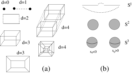
Figure 1: (a) Construction of a $d$-dimensional cube (hypercube) by combining pairs of $(d-1)$-dimensional cubes. The dotted lines are the new connections or bonds. (b) Hyperspheres may also be constructed that way. Take two closed intervals with the identification of the boundary points as indicated by the dashed lines to get $S^{1}$. Similarly, two full spheres $B^{d}$, unit $d$-balls, one for $x_{0}<0$ and another one for $x_{0}>0$ with the identification of the boundaries gives $S^{d}$. E.g., take two disks ($d=2$) and place one top of the other both centered at origin. Since the boundaries are identified, puff the object (think of making luchi [https://en.wikipedia.org/wiki/Luchi]) giving an extra dimension as $x_{0}=\pm\sqrt{1-\sum_{i=1}^{d}x_{i}^{2}}$, the boundary being at $x_{0}=0$. The net result is $S^{d},$ $\sum_{i=0}^{d}x_{i}^{2}=1$. This construction is not possible for solid cubes or solid balls.

3.1 Euclidean dimension

A common procedure is to embed the lattice in an Euclidean space of large enough dimensions. From any point, draw a sphere of radius $R$ and count the number $N$ of points enclosed by the sphere. Our expectation is that, for a $d$-dimensional set, $N\sim R^{d}$. Exploiting this intuition, a definition of $d$ can be

$$d=\lim_{R\to\infty}\frac{\ln N}{\ln R},\qquad({\rm Euclidean})$$ (1)

the asymptotic slope of a log-log plot of $N$ vs $R$. The above definition may be written in a more useful form as

$$R\;\frac{\partial N(R)}{\partial R}=d\;N(R),$$ (2)

where the coefficient of the linear term on the right hand side corresponds to the dimension of the space.

An equation like Eq. (2) is suggestive of the form used in renormalization group approach and can be linked to dimensional analysis for various physical quantities. If a physical quantity $A$, on dimensional grounds, depends on length as $L^{c}$, then there is an equation equivalent to Eq. (2), viz.,

$$L\;\frac{\partial A}{\partial L}=c\;A,$$ (3)

where $c$ will be called the engineering dimension of $A$.

3.1.1 $d$ via analytic continuation

In many problems, especially in renormalization group calculations ($\epsilon$-expansion), one generalizes the Euclidean dimension, Eq. (1), to a continuous variable. This is more of an analytic continuation with the help of the metric than by any real construction of any space. A Gaussian integral in $d$ dimensions can be written as

$$\int e^{-ar^{2}}d^{d}r=K_{d}\int_{0}^{\infty}e^{-ar^{2}}r^{d-1}dr,\quad{\rm with}\quad K_{d}=\frac{2\pi^{d/2}}{\Gamma(d/2)},$$ (4)

as the surface area of a unit sphere. An integration like the left hand side of Eq. (4) above is metric dependent. Once converted to a one-dimensional integral of a function where $d$ appears as a parameter (like the right hand side of Eq.(4)), it is defined for any value of $d$ allowing an analytic continuation to the whole complex plane of $d$. This is very useful to handle singularities or divergent integrals (dimensional regularization) in many problems. In this analytic continuation approach, there is no association of any space with noninteger $d$ and so we do not get into detailed discussion on this approach in this chapter. (See Prob 3.1).

3.2 Topological dimension

It is possible to avoid any reference to an embedding space by using the intrinsic characteristics of the lattice. By lattice we mean a set of points connected by bonds and these bonds can be taken as a unit or a scale for the connectivity of the points. We take an $L$ step path on the lattice from any one point and count all the new points visited that were not seen upto the $(L-1)$th step. This is like counting the boundary points of an intrinsically defined sphere of radius $L$. Based on the expectation that the boundary “area” grows like $N_{b}\sim L^{d-1}$, the definition of the dimension is

$$d_{\rm t}=1+\lim_{L\to\infty}\frac{\ln N_{b}}{\ln L}.\qquad({\rm topological})$$ (5)

This will be called the topological dimension of the object. It is topological because this number does not change under continuous deformation of the space. In other words two homeomorphic spaces have the same topological dimension.

A formal definition of the topological dimension is via the covers. A crude definition is that if $\delta$ is the dimension of the space (or lowest dimension of all possible spaces) that separates our space into disconnected pieces, then the topological dimension of our space is $1+\delta$.

We make a convention that a null set $\emptyset$ has dimension $-1$ while a point set has dimension $0$. All others follow from the above rule.

There are ambiguities. As an example, take a line. A line is broken into two pieces by removing a point. A point by definition is of zero dimension. Hence a line is a one-dimensional object. This is however a bit tricky. If we think of a line in three dimensions, it can be broken into two pieces by another line or by a plane etc. In such situations, we need to choose the smallest dimensional object to determine $\delta$. Another example could be a figure $\Large{\overline{\bullet}}$ ( a line and a disk). Being disconnected, a null set separates them, and, therefore, the dimension should be $1+(-1)=0$. But individually these are 1 (line) and 2 dimensional (disk) spaces. In such a situation we define a local dimension and choose the largest one. In this particular case it will be $d=2$.

The above rules may be formalized by an iterative procedure with the basis sets of the space. (a) If the boundaries of the basis sets are of dimensions $\leq d-1$, then the space is of dimension $\leq d$. (b) If this is true for $d$ but not for $d-1$, then the space has dimension $d$.

For the disk-bar example above, the basis sets for the bar has boundaries $d=0$ while the disk has basis sets with boundaries $d=1$, i.e., the dimension of the boundaries of the basis sets satisfy $d\leq 1$. Therefore $d\leq 2$. Invoke (b) to rule out $d=1$ or any number greater than 2.

Let us take $R$ with the usual topology defined by the open sets $(a,b),b>a$. The boundaries are 0-dimensional points for all such open sets. Hence $R$ has dimension $d=1$. With inherited topology for $S^{1}$, the basis sets (open arcs of a circle) have boundaries of dimensionality $0$. Therefore $S^{1}$ has $d=1$.

All the definitions used so far would give the dimension of $R^{d}$ to be $d$. This number $d$ happens to be the number of independent vectors needed to span the space when viewed as a vector space. The dimensionality of a topological space is a topological invariant in the sense that if there is a continuous mapping or homeomorphism that takes $R^{m}$ to $R^{n}$, then $m=n$.

Problem 3.1:

A problem on dimensional regularization. Show that the one-dimensional integral $I_{1}(x)=\int_{-\infty}^{\infty}\frac{dz}{\sqrt{x^{2}+z^{2}}}$ is divergent.

To tackle this divergence, generalize the integral to $d$ dimensions as

$$I_{d}(x)=\int_{-\infty}^{\infty}...\int_{-\infty}^{\infty}\frac{d^{d}r}{\mu^{d-1}\sqrt{x^{2}+r^{2}}}=K_{d}\int_{0}^{\infty}\frac{r^{d-1}dr}{\mu^{d-1}\sqrt{x^{2}+r^{2}}},$$ (6)

where an arbitrary length $\mu$ is introduced to maintain the correct dimensions (engineering dimension!). Formally, $I_{d}$ is $I_{1}$ for $d=1$. The form on the right hand side can be defined for any $d$. With $d$ as a continuous variable, the integral is divergent for $d\geq 1$ but convergent for $d<1$. This signals the possibility of a singularity in the complex $d$-plane at $d=1$. By doing the integral in the convergent domain in the $d$-plane, show, by using Gamma functions and analytic continuation, that

$$I_{d}(x)=\left(\sqrt{\pi}\frac{x}{\mu}\right)^{d-1}\ {\Gamma\left(\frac{1-d}{2}\right)}=\frac{2}{\epsilon}-2\ \ln(x/\tilde{\mu})+O(\epsilon),$$ (7)

where $\epsilon=1-d$ is a small parameter for the expansion. Absorb some O(1) factor in $\mu$ to define $\tilde{\mu}$.

This particular example appears in the calculation of the electrostatic potential due to an infinitely long uniformly charged wire.

Problem 3.2:

(Mathematical) Show that the definition of $d$ obtained by using a basis is independent of the basis chosen.

One way of doing it is to define $d$ without any basis but with the help of the open sets. The iterative definition of the dimension of a topological space $T$ for a set $X$ would be as follows: The dimension is $d$ if for any point $x\in X$ and any set $U\in T$ containing $x$, there exists an open $V$ with $x\in V$ such that the closure of $V$ is contained in $U$ with dim$(\partial V)\leq d-1$. If this is satisfied for $d$ but not for $d-1$, then the dimension of the space is $d$. It is assumed that dim$(T)$=-1 if $X=\emptyset$.

Problem 3.3:

(Mathematical) Prove that if $R^{m}$ is topologically equivalent (i.e. homeomorphic) to $R^{n}$, then $m=n$. This means the dimension is a topological invariant.

4 Fractal dimension: Hausdorff, Minkowski (box) dimensions

Let us now look at some nontrivial examples. We shall see that topological dimension ($d_{\rm t}$) is not enough; a few others are needed. First among these is the Hausdorff dimension ($d_{\rm f}$) that one gets by embedding the set in a real space $R^{n}$ of appropriate dimension $n$.

In the following the Cantor set (defined below) is taken as a paradigmatic example because of its apparent simplicity. It is an example of a space of topological dimension 0 but it is not just a finite collection of points.

4.1 Cantor set: $d_{\rm t}=0,d_{\rm f}<1$

There are many ways to define Cantor sets. The middle $1/3$ rule used below is historically the first one defined by Cantor and will be called the Cantor set.

Figure 2: Construction of a cantor set

The set is constructed iteratively by taking a closed interval 0 to 1, and then removing the middle 1/3 to get two closed intervals. In the next step, the middle one third of the two branches are removed leaving us with 4 intervals (Fig. 2). This iterative process leaves a set of disconnected points,

$$\left.\begin{array}[]{lcl}S_{0}&=&\left[0,1\right],\\ S_{1}&=&\left[0,\frac{1}{3}\right]\cup\left[\frac{2}{3},1\right],\\ S_{2}&=&\left[0,\frac{1}{9}\right]\cup\left[\frac{2}{9},\frac{3}{9}\right]\cup\left[\frac{6}{9},\frac{7}{9}\right]\cup\left[\frac{8}{9},1\right],\\ ...\end{array}\right\}\quad{\cal S}=\cap_{n=0}^{\infty}S_{n}.$$ (12)

First note that the lengths of intervals removed are successively $\frac{1}{3},\frac{2}{3^{2}},...$ so that the total length removed is $\sum_{n}\frac{2^{n-1}}{3^{n}}=1$. Since the total length we started with is $1$, the remaining points have no “length” and therefore cannot be one-dimensional. The set is disconnected. Therefore the topological dimension is $d_{\rm t}=0$. Despite this 0-dimensionality, there is still a nontrivial structure like self-similarity. If any one part of the $n$th iterate is multiplied by $3$, we get back the state in the $(n-1)$th iterate. This geometric structure is described by a different dimension, to be called the self-similarity dimension or box dimension or Hausdorff dimension.

For a regular object like the Cantor set, the pattern is obtained by scaling the $n$th iterate by a scale $b<1$ and combining $C_{b}$ of them. Here, $b=1/3$ and $C_{b}=2$. On successive rescaling how the number grows is given by the Hausdorff dimension

$$d_{\rm H}=\frac{\ln(C_{b})}{\ln(1/b)}.\qquad{\rm(Hausdorff)}$$ (13)

For the Cantor set, $d_{\rm H}=\frac{\ln 2}{\ln 3}\approx 0.63<1$. We have assumed a power law dependence, $C_{b}\sim b^{-d_{\rm H}}$.

Another practical procedure is to cover the set by boxes. Consider the set as a part of $R^{d}$. Cover it by boxes of length $L$ and count the number of boxes occupied by the set. Let this be $B_{L}$. If the length is changed to $bL$ by a scale factor $b<1$, the number changes to $B_{bL}$. The box dimension is then defined as

$$d_{\rm f}=\lim_{n\to\infty}\frac{\ln(B_{b^{n}L}/B_{L})}{\ln(1/b^{n})}.\qquad{\rm(Box\;\;or\ Minkowski)}$$ (14)

By using successive generations, we may also write the above equation as

$$d_{\rm f}=\lim_{n\to\infty}\frac{\ln(B_{b^{n}L})-\ln(B_{b^{n-1}L})}{\ln(1/b^{n})-\ln(1/b^{n-1})},\qquad{\rm(Box\;\;or\ Minkowski)}$$ (15)

which is the discrete version of Eq. (2).

For the Cantor set, if we choose $b=1/3$, then $B_{b^{n}}=2^{n}$, and, therefore, $d_{\rm f}=\frac{\ln 2}{\ln 3}=\log_{3}2=d_{\rm H}$. The box dimension is also called the Minkowski dimension.

The occurrence of $\ln 3$, or log base $3$, is not accident. It comes from the scale $1/3$ under which the Cantor set is scale invariant. If we choose an arbitrary scale factor, say $b=1/2.9$, the scale invariance of the Cantor set is not obvious. This existence of a special scale, here $1/3$ or its powers, is an example of discrete scale invariance. In Appendix we discuss how a discrete scale invariance leads to complex dimensions.

Figure 3: Covering by boxes. Count the number of boxes required to cover the object for different box sizes like those represented by the solid grid and the dotted grid. The dotted grid is finer and therefore would involve larger number of boxes.

Whenever the Hausdorff dimension is different from the topological dimension, the set is called a fractal. For most regular fractals, $d_{\rm H}=d_{\rm f}$, but there are cases where they may differ. When they are same, they may be called the fractal dimension or the scaling dimension.

A subtle difference in the way the Hausdorff and the Minkowski dimensions are defined may be noted here. The Hausdorff dimension is obtained by going to the large size limit by scaling up the structure, while the Minkowski dimension is from the opposite limit. In the latter case, one explores to the short scale behaviour by using progressively smaller boxes. From an experimentalist’s point of view, the Hausdorff dimension is obtained when probed in the long wavelength limit, called the infrared limit, while the Minkowski (box) dimension is obtained when probed using shorter wavelengths, called the ultraviolet limit.

4.1.1 When Hausdorff$\neq$ Minkowski

An example of a case of different Hausdorff and Minkowski dimension is the set of rational numbers in $(0,1)$. If we want to cover this set by linear “boxes”, every box will contain some points. It follows from the fact that the rationals form a dense set in $(0,1)$. Therefore the box dimension or Minkowski dimension is one. On the other hand, each rational number is an isolated point with dimension zero. A countable union of points will then have a Hausdorff dimension of zero. Generally if $F$ is a dense subset of an open region of ${\mathbb{R}}^{n}$, then its box dimension is $n$. Note however that Cantor set does not belong to this category because it is uncountable.

4.1.2 Inhomogeneous scaling

Let us write the definition of $d_{\rm H}$ in Eq. (13) in a different way as $C\lambda^{d_{\rm f}}=1$, where $\lambda(=1/b)<1$ is the scale factor and $C$ is the number of such scaled objects combined to generate the next generation. This equation may now be extended to a situation of inhomogeneous scaling where each of the $C$ objects has its own scale factor $\lambda_{i}<1$. The fractal dimension is then the solution of the equation $\sum_{i=1}^{C}\lambda_{i}^{d_{\rm f}}=1$.

4.1.3 Fractal dimension as a Continuous variable

Instead of the 1/3 rule of the Cantor set, we may remove any open interval $(x,1-x),x<1/2$. After that we remove the appropriate $(1-2x){\cal L}$ part from each of the remainders of length ${\cal L}$. Let’s call it th $x$-rule. For $b=x$, $C_{b^{n}}=2^{n}$. The fractal dimension is

$$d_{\rm f}(x)=\frac{\ln 2}{\ln(1/x)},\qquad{\rm(continuous)}$$ (16)

with $d_{\rm f}(x=0)=0,d_{\rm f}(x=1/2)=1$ as expected. It is therefore possible to construct a family of fractals with fractal dimension $d_{\rm f}$ as a continuous variable in the range $[0,1]$.

Fractals of dimension $d_{\rm f}>1$ can be constructed by taking advantage of product spaces. Given a $1<d_{\rm f}<m$, where $m$ is an integer ($>1$), use the $x$-rule to construct a fractal ${\cal F}$ of $d_{\rm f}^{\prime}=d_{\rm f}/m<1$. Then construct the direct product space ${\cal F}\times...\times{\cal F}$. For the scale factor $b$, we now need $m$-dimensional boxes so that the number of boxes covered is $C_{bL}^{m}$. The fractal dimension, by Eq. (14), is $m\;d_{\rm f}^{\prime}=d_{\rm f}$.

Since $m$ can be any integer greater than the chosen value of $d_{\rm f}$, we end up with many different product spaces all of the same fractal dimension $d_{\rm f}$. Therefore, $d_{\rm f}$ is a necessary but not a sufficient characterization of the space.

4.1.4 Configuration space of the Ising model

We raised the question of the configuration space of the Ising model which consists of $N$ spins $s_{i}=\pm 1$. For each spin we have a discrete topological space $\{0,1\}$ so that for infinitely many spins arranged in a one-dimensional lattice, the total configuration space is a product space $\{0,1\}^{Z}$. We now show that the configuration space can be mapped on to a set of real numbers $\in[0,1]$, whose fractal dimension can be determined.

Let us first consider a particular case using ternary expansion of numbers. By construction, any member of the Cantor set can be expressed as

$$y=\sum_{n=1}\frac{a_{n}}{3^{n}},\quad{\mathrm{where}}\quad a_{n}=0\;{\rm or}\;2.$$ (17)

This is because every point in $S_{n}$ exists in all the previous generations. Therefore any point can be tracked as belonging to either the 0th or the 2nd interval of the previous step. Equivalently, the points can be represented by an infinite string $(a_{1}a_{2}a_{3}....a_{n}....)$, like $(02220220002....)$ , or by dividing by 2, an infinite string of 0’s and 1’s. For an infinitely long chain of Ising spins, a configuration $(s_{1}s_{2}...s_{n}...)$ can be converted to a real number

$$x=\sum_{n=1}^{\infty}\;\frac{2s_{n}}{3^{n}},\quad{\rm with}\quad s_{n}=0,1,$$ (18)

similar to Eq. (17). In other words, the topological space of the Cantor set can be mapped on to $\{0,1\}^{Z}$, or, equivalently, can be mapped onto the configuration space of an infinitely long Ising chain.

The entropy per spin of the Ising model in the high temperature limit is $k_{B}\ln 2$ where $k_{B}$ is the Boltzmann constant What we learn from this analysis is that the entropy (in this case the high temperature entropy) of the Ising system (or, for that matter, any two state model) is determined by the dimension $\log_{3}2$ of the set of real numbers equivalent to the configuration space . The connection between the dimension of the equivalent set of real numbers and the entropy is discussed in Appendix A where we also show that base $3$ is nothing special.

Problem 4.1:

The Ising two state problem can be mapped on to the Cantor set as the collection of all infinite strings of 0 and 1 occurring with equal probability. Suppose, instead, 0 occurs with probability $p$, and 1 with $q=1-p$. The physical entropy per spin is known to be $s=-k_{B}(p\ln p+q\ln q)$, where $k_{B}$ is the Boltzmann constant. Show that the fractal dimension of the set of real numbers is $d_{\rm f}\propto S$, because $d_{\rm f}=-(p\ln p+q\ln q)/\ln 3.$

Problem 4.2:

A generalization of the above problem is to consider the set of all strings of base $m$ numbers, i.e., strings of $0,1,...m-1$. A string $\{a_{n}\},a_{n}=0,1,...m-1$, corresponds to a real number $x=\sum_{1}^{\infty}a_{n}/m^{n}$. If the digits $0,1...m-1$ occur with probabilities $p_{n},n=0,...,m-1$, then the fractal dimension of the et consisting of $x$’s is $d_{\rm f}=-(\sum_{n}p_{n}\ln p_{n})/\ln m$.

A consequence of this result is that if only $s_{n}=0,1$ occur with probabilities $p,q=1-p$, then $d_{\rm f}=-(p\ln p+q\ln q)/\ln m$,, e.g., for the set $x=\sum_{n}(m-1)s_{n}/m^{n}$ (a generalization of the standard Cantor set).

Problem 4.3:

Consider the infinitely long Ising chain configurations, but now with a restriction that no two 0’s can be adjacent (or nearest neighbours). This occurs in nonabelian anyon chains discussed in later chapters. (See Ref. [5]). For $N$ spins, the total number of configurations is not $2^{N}$ any more. If $C_{N}$ is the number of $N$ spin configurations under this restriction, then show that $C_{N}=C_{N-1}+C_{N-2}$.
Hint: If the first spin is 1, then the second onwards can be any of the allowed $N-1$ spin configurations. This is $C_{N-1}$. If the first one is 0, then by restriction, the next one has to be 1 but the spins are free after that. The number of such configurations is $C_{N-2}$. Note that $C_{1}=1,C_{2}=3$. This is the Fibonacci sequence.

If $C_{N}\sim\tau^{N}$ for large $N$, then show $\tau=(1+\sqrt{5})/2$ (golden mean), as expected for the Fibonacci numbers. Show that the fractal dimension of the corresponding real number set is $\propto\ln\tau$ (see problems 4.1 and 4.2).

A number like $\tau$ here, different from the standard value $2$, is often called the quantum dimension of the anyonic chain, . Suppose we consider spin-1/2 particles. For each spin the Hilbert space is 2 dimensional. Then the Hilbert space for $N$ spins is the tensor product with dimensions $2\times 2\times 2...=2^{N}$. In contrast for the (Fibonacci-) anyon chains, even though individually the spaces are two dimensional, the dimension of the $N$-anyon Hilbert space is $\tau^{N}$ for large $N$. This is as if the effective dimension of individual Hilbert space is $\tau$. To recognize this difference, this dimension is called “quantum dimension”. It is interesting to note that the topological entanglement entropy is determined by $\ln\tau$. This goes beyond the scope of this chapter.

Problem 4.4:

What is the configuration space of Ising spins on a square lattice? Explore if there is any mapping to real numbers, or any connection with the fractal dimension of the set of numbers, as found for a one dimensional chain of spins.

4.2 Koch curve: $d_{\rm t}=1,d_{\rm f}>1$

A Koch curve is defined in Fig. 4. Instead of deleting the middle $1/3$ as in the Cantor set, we add an extra piece increasing the length of the line. This curve has the following properties:

1. A point disconnects it. Therefore it has a topological dimension $d_{\rm t}=1$.

2. The generation-wise lengths are $1,\frac{4}{3},\left(\frac{4}{3}\right)^{2},...\left(\frac{4}{3}\right)^{n},...$ so that the length $L_{n}\to\infty$ as $n\to\infty$. However the area under the curve is $1+\frac{4}{9}+\left(\frac{4}{9}\right)^{2}+...=\frac{9}{5}$.

3. For a stick length $l_{n}=1/3^{n}$, the number of sticks is $C_{n}=4^{n}$. For a scale factor $b=1/3$, the ratio of the two numbers $C_{n+1}/C_{n}=4$. The fractal dimension is $d_{\rm f}=\lim_{n\to\infty}\frac{\ln(C_{n}/C_{n-1})}{\ln(1/b)}=\frac{\ln 4}{\ln 3}$

A practical procedure is to cover the curve with a square grid of unit length $l=1$ and count the number of boxes $C_{l}$ occupied by the curve. Then change the grid size by a scale factor $b$ and count $C_{bl}$. One may then use the slope of the log-log plot with the definition of Eq. (14) to determine $d_{\rm f}$.

Figure 4: (a)Iterative construction of the Koch curve. An interval of length 1 is divided into 3 equal parts. The middle segment is replaced by an equilateral triangle of side length 1/3 without the base. This procedure is repeated for each segment. The length of the curve ($L_{n}$) and the area ($A_{n}$) under it for the first few generations are given. (b) Similar construction with a triangle. After infinite iteration we get a closed loop of infinite perimeter but of finite area. This is equivalent to $S^{1}$ where “1” refers to the topological dimension.

If we take $\epsilon=1/3^{n}$ as the length of the measuring stick with $\epsilon\to 0$ as $n\to\infty$, then the measured length $(4/3)^{n}$ is dependent on the scale via $n=-\ln\epsilon/\ln 3$. We may generalize this result. The length measured at scale $\epsilon$ behaves as

$$L(\epsilon)\stackrel{{\scriptstyle\epsilon\to 0}}{{=}}L_{0}\epsilon^{-\alpha},\quad{\rm with\ }\alpha=d_{\rm f}-d_{\rm t}.$$ (19)

For those cases where the two dimensions match (as in $R$), the length is independent of the scale. In such cases, one may talk of the length of the curve, and such curves are called rectifiable curve.

We see a curve of topological dimension 1 but of a fractal dimension between 1 and 2. Koch curve is also an example of a continuous but nowhere differentiable curve. As a closed curve, Fig. 4b, we get a continuous curve enclosing a finite area, though of infinite length. Fig. 4b is therefore topologically equivalent to $S^{1}$, where we now recognize the superscript as the topological dimension of the boundary.

Problem 4.5:

Construct a space filling curve, i,e, a curve of topological dimension 1 but of fractal dimension 2. An example is the Peano curve. See Ref. [4].

4.3 Sierpinski Gasket: $d_{\rm t}=1,d_{\rm f}>1$

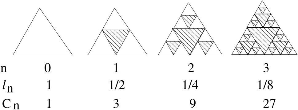
Figure 5: (a)Iterative construction of the Sierpinski gasket. One way is to view it as an aggregation of triangles so that the side length increases by a factor of 2, with the inner one missing (shaded triangles). Another view is to punch holes and remove the inner 1/3 of every triangle. The length for counting ($l_{n}$) and the number ($C_{n}$) of triangles are noted underneath.

The construction of the Sierpinski gasket is shown in Fig. 5. This fractal can be disconnected by isolated points and is therefore topologically one-dimensional.

A fractal that can be disconnected by a finite set of points is called a finitely ramified fractal. A finitely ramified fractal is therefore has a topological dimension 1. The fact that we need 3 copies at a scale factor of 2 tells us that the fractal dimension of the Sierpinski gasket is $d_{\rm f}=\frac{\ln 3}{\ln 2}$.

An intuitive way of arguing that its fractal dimension is less than 2 is to note that there are holes at every scale, and therefore holes will be present no matter at what resolution we look at, unlike a compact object. This of course requires $n\to\infty$.

Problem 4.6:

Show that the Sierpinski gasket is topologically equivalent to $S^{1}$ but it is not rectifiable (i.e., its length $\to\infty$).

Problem 4.7:

Sierpinski Carpet: Take a square of side length 1. Divide each side into three pieces of length 1/3 and remove the inner square of area 1/9. Repeat this process ad infinitum.

(a) Show that the total area is zero.

(b) Show that the carpet consists of points with a ternary expansion $(\sum_{n=1}^{\infty}\frac{a_{n}}{3^{n}},\sum_{n=1}^{\infty}\frac{b_{n}}{3^{n}})$ where $(a_{n},b_{n})\in{\cal S}$, ${\cal S}=\{0,1,2\}\times\{0,1,2\}-\{(1,1)\}$. The topological space is ${\cal S}^{Z_{+}}$.

(c) Identify the Cantor sets along the diagonal and the medians.

(c) Show that the fractal dimension is $d_{\rm f}=\frac{\ln 8}{\ln 3}$.

(d) Show that it is an infinitely ramified fractal, but with topological dimension = 1. Note that the topological dimension by definition is an integer. For the carpet, it has to be less than $2$, and it is not $0$. Hence it is $1$. Construct a direct proof of this.

(e) Show that the Sierpinski Gasket can be homeomorphically embedded in the Sierpinski carpet. Prove a more general statement: “any Jordan curve can be homeomorphically embedded in the Sierpinski carpet.” This was proved by Sierpinski in 1916.

Problem 4.8:

Hierarchical lattices

A hierarchical lattice is built by successive replacement of a bond by a motif. In the example the motif consists of a diamond like object with $b$ branches and $2b$ bonds. This is also called a diamond hierarchical lattice. Show that the fractal dimension is $d_{\rm f}=\frac{\ln 2b}{\ln 2}$.

The hierarchical construction of such lattices helps in easy implementation of renormalization group transformations or scaling.

4.4 Paths in Quantum mechanics:$d_{\rm t}=1,d_{\rm f}=2$

We now argue that the trajectories of a nonrelativistic quantum particle is a fractal obeying Eq. (19). The traditional Brownian motion also belongs to the same class.

From the uncertainty principle, fluctuations in position ($\delta x$) and momentum ($\delta p$) are related by $\delta x\;\delta p\sim\hbar$ and $\delta p=m\delta x/\delta t$, ($t$ being time), it follows that

$$(\delta x)^{2}\sim\delta t.$$ (20)

Take these $\delta x,\delta t$ as the scales for space and time to measure the length of a trajectory from $(x_{1},t_{1})$ to $(x_{2},t_{2})$. The time interval $T=t_{2}-t_{1}$ consists of $N=T/\delta t$ pieces so that the length is

$$L=N\ \delta x=\frac{T}{\delta t}\delta x=\frac{T}{\delta x},$$ (21)

where Eq. (20) has been used. Therefore, $L\to\infty$ as $\delta t\to 0$. We conclude, by comparing with Eq. (19), that the fractal dimension of the trajectory is $d_{\rm f}=2$, though a path, by definition, has a topological dimension $d_{\rm t}=1$.

Problem 4.9:

For the cases where the propagator in the path integral approach can be calculated exactly, it is observed that only the classical path contributes. By definition, a classical path has $d_{\rm f}=d_{\rm t}=1$. Show that this happens because of the interference of the nearby quantum paths.

5 Dimensions related to physical problems

To go beyond topology and geometry, we need to study some physical problem on a fractal. These could be of several types as mentioned in Sec. 2. Let’s consider those cases one by one.

5.1 Spectral dimension

A physical way to explore a space is to use a probe that would in principle involve the whole space. In Euclidean space, a few such probes are (1) diffusion processes or random walks, (2) elastic waves or lattice vibration and (3) any quantum mechanics problem. The common link among the three types is via the Laplacian in the Euclidean space as follows.

1. The diffusion process is described by the differential equation for any diffusing field $\psi$,

   $$\frac{\partial\psi}{\partial t}=D\nabla^{2}\psi,$$ (22)

   where $D$ is the diffusion constant.

2. The free particle Schrödinger equation is described by

   $$i\hbar\frac{\partial\psi}{\partial t}=-\frac{\hbar^{2}}{2m}\nabla^{2}\psi,$$ (23)

   where $m$ is the mass of the particle and $\hbar$ is the Planck constant divided by $2\pi$.

3. The wave equation, e.g., describing sound waves is

   $$\frac{\partial^{2}\psi}{\partial t^{2}}=c^{2}\nabla^{2}\psi.$$ (24)

The diffusion equation also occurs in heat transport and defining the Laplacian for any space is often called the heat-kernel problem. For some of the fractals, it is easier to consider the lattice vibration problem or the scalar version the resistor problem in the zero frequency limit. Th dimensionality of the space can then be defined by the appropriate generalization of the Euclidean results. This we do below. The dimension we obtain in this way is called the spectral dimension $d_{s}$.

5.1.1 Diffusion, random walk

For a diffusion problem in $\mathbb{R}^{d}$ the probability distribution of the end to end vector ${\bf R}$ is a Gaussian

$$P({\bf R})=\frac{1}{(2\pi t)^{d/2}}\ \exp\left(-\frac{dR^{2}}{2t}\right)\equiv\frac{1}{(2\pi t)^{d/2}}\ f(R/\sqrt{t}).$$ (25)

In this limit short scale details are not expected to be important. A general form allowing a dimensionality dependence is to write it as

$$P({\bf R})\sim{t}^{-d_{s}/2}\ f(R/\sqrt{t^{1/d_{w}}}),$$ (26)

defining a walk dimension $d_{w}$ and a spectral dimension $d_{s}$. For $\mathbb{R}^{n}$, $d_{s}=n,d_{w}=2$. Since probability is normalized, where the integration over ${\bf R}$ involves the fractal dimension, a change of variable gives

$$\int d^{d_{\rm f}}R\;P({\bf R})\sim t^{d_{\rm f}/d_{w}-d_{s}/2}.$$

Since the power of $t$ should be zero, it follows that

$$d_{s}=2\frac{d_{\rm f}}{d_{w}}.$$ (27)

Only for $d_{w}=2$, the Hausdorff and the spectral dimensions match. This turns out to be the case for hierarchical lattices of Prob. 3.6.

Based on Eq. (26), the spectral dimension can be defined from the return to origin probability $P(0,t)$ as

$$d_{s}=-2\lim_{t\to\infty}\ \frac{\ln P(0,t)}{\ln t}.$$ (28)

As for the paths in quantum mechanics (Sec. 4.4), $d_{w}$ is the fractal dimension of the walk. It may also be seen as the scaling relation between space rescaling and time rescaling as determined by the dynamics. In such contexts, $d_{w}$, denoted by $z$, is called the dynamic exponent. For diffusion like processes $z=2$. The dynamic exponent is an important characteristic quantity near various phase transitions.

5.1.2 Density of states

For a quantum mechanical problem with energy dispersion relation $\omega=Ck^{p}$ for small wave vector $k=|{\bf k}|$ in $d$ dimensions, the density of states for $\omega\to 0$ is $\rho(\omega)\sim\omega^{-1+d/p}$, with the integrated density of states as $I(\omega)\sim\omega^{-d/p}$. For the electronic problem with a quadratic dispersion relation, $p=2$ and one gets $\rho(\omega)\sim\omega^{-1+d/2},I(\omega)\sim\omega^{d/2}$. For phonons, $p=1$ and so, $\rho_{\rm phonon}(\omega)\sim\omega^{d-1}$, which gives the Debye law for specific heat. The low energy excitations involve $k\to 0$ (long wavelength) for which small scale details do not matter. In other words, the large scale dynamical features of the fractal or the object are probed by the long wavelength propagation. As a generalization, $d$ in the above densities may be replaced by $d_{s}$ which is called the spectral dimension.

It is shown in Appendix B that $d_{s}$ for the Sierpinski Gasket is different from its fractal dimension by explicitly calculating the spectral dimension.

6 Which $d$?

We now go back to the questions asked at the beginning of this chapter, Sec. 2.

6.1 Thermodynamic equation of state

The thermodynamic relation alluded to at the beginning actually comes from the density of states. In the grand canonical ensemble, the grand potential (the equivalent of free energy) is $-PV$, and for a noninteracting gas, it can be written as

$$PV=k_{B}T\int d\epsilon\;\rho(\epsilon)\;\ln{\cal{Z}}(\epsilon,\beta,\mu),$$ (29)

where $\epsilon$ is the energy, $\rho(\epsilon)$ the density of states, $\beta=1/k_{B}T$ the inverse temperature, $\mu$ the chemical potential, and ${\cal{Z}}$ is the single state grand canonical partition function,

$${\cal{Z}}=\sum_{n=0}^{\infty}g_{n}\exp[-\beta(\epsilon-\mu)n],$$ (30)

where

$$g_{n}=\left\{\begin{array}[]{cl}1,&{\mathrm{for\ bosons,}}\\ (n!)^{-1},&{\mathrm{for\ classical\ particles,}}\\[4.0pt] \left[\begin{array}[]{ll}1,&{\mathrm{if}}\ n=0,1\\ 0,&{\mathrm{if}}\ n>1\end{array}\right.&{\mathrm{for\ fermions,}}\end{array}\right.$$ (31)

though the explicit form is not required for our argument.

The average particle number and the average energy are then given by

$$\langle N\rangle=\int d\epsilon\;\rho(\epsilon)\;{\overline{n}}(\epsilon,\beta,\mu),\quad{\mathrm{and}}\quad U=\int d\epsilon\;\rho(\epsilon)\;\epsilon\;{\overline{n}}(\epsilon,\beta,\mu),$$ (32)

where

$${\overline{n}}(\epsilon,\beta,\mu)=k_{B}T\frac{\partial\ln{\cal{Z}}}{\partial\epsilon}.$$ (33)

We now take the definition of spectral dimension to write $\rho(\epsilon)=A\epsilon^{-1+d_{s}/2}$ for free particles of mass $m$ with a dispersion relation $\epsilon=p^{2}/2m$, with $A$ some constant. The density of states may be divergent but is always integrable. With these information in hand, an integration by parts of the integral for $U$ in Eq. (32), in conjunction with the (negative) grand potential in Eq. (29) gives us the required relation

$$PV=\frac{2}{d_{s}}U.$$ (34)

The thermodynamic fundamental relation for an ideal gas involves the spectral dimension of the space.

6.2 Phase transitions

The notion of lower critical dimension arose from studies of symmetry breaking in various dimensions. See Ref. [7] for an introduction to critical phenomena.

Two different cases are to be considered, namely a discrete or a continuous symmetry breaking. To be concrete, it is better to consider a particular case. A typical Hamiltonian is $H=-J\sum_{<ij>}{\bf S}_{i}\cdot{\bf S}_{j}$ where ${\bf S}_{i}$ is a unit $n$-component spin vector at site $i$ of say a hypercubic lattice. For the Ising model $S_{i}=\pm 1$ is just a discrete variable with $n=1$. Continuous cases correspond to $n\geq 2$; the planar xy model has $n=2$, the three dimensional spin $n=3$ is the Heisenberg ferromagnet, etc. The Hamiltonian allows an ordered ground state where all spins are parallel. Therefore at zero temperature ($T=0$) we get a ferromagnetic state that breaks the rotational invariance of $H$. Note that $H$ remains invariant under a rotation of the spins by any amount if performed on all the spins (global symmetry). For the Ising case, the symmetry is discrete with $S_{i}\to-S_{i}$. As we raise temperature, thermal fluctuations tend to destroy the perfect alignment of spins due to entropic reasons. Therefore the question arises whether the broken symmetry state persists at nonzero temperatures. It is known that at very high temperatures entropy wins yielding a paramagnetic phase. In case the ordered state persists, then there has to be a special temperature $T=T_{c}$ (called the Curie point) at which a phase transition takes place. If we look at this particular $H$ in various dimensions, then $T_{c}\neq 0$ only for $d>d_{l}$, where $d_{l}$ is called the lower critical dimension. For the Ising case, $d_{l}=1$ while for $n\geq 2$, $d_{l}=2$. For a fractal, to which $d$ are we referring?

6.2.1 Discrete case: Ising model

The Landau-Peierls argument for the Ising Hamiltonian is a generic way of determining the lower critical dimension for discrete symmetry breaking. Let us start with an ordered state, say all up spins at $T=0$, and isolate a domain of opposite spins (down spins). By symmetry, the two states have the same energy, and, therefore, the cost of flipping the spins is in the creation of the boundary. Furthermore, same number of down spins can be enclosed by boundaries of different shapes. The boundary therefore has an entropy associated with it. Since the boundaries define the topological dimension of the system, we may write the change in free energy as

$$\Delta F=\sigma L^{d_{\rm t}-1}-Ts_{0}L^{d_{\rm t}-1},$$ (35)

where $\sigma$ is the energy cost of creating a unit “area” boundary and $s_{0}$ is the associated entropy. E.g., for the Ising case on a square lattice, $\sigma=2J$. The free energy expression in Eq. (35) is valid for $d_{\rm t}>1$ for which such flipped domains may not destroy the ordered state if $T<\sigma/s_{0}$. Thus a ferromagnetic state with broken symmetry can exist at nonzero temperatures. If $d_{\rm t}=1$, the cost in energy is independent of the size but the flipped block can be placed anywhere on the lattice giving an entropy $\propto\ln N$ where $N$ is the size of the system. For large $N$, entropy dominates, and so the system goes over to a paramagnetic state at any nonzero $T$. The lower critical dimension is therefore one, and it is the topological dimension that matters. This means the Ising model on a Sierpinski Gasket does not show a ferromagnetic state.

The above simple picture is not complete, because we have seen that the topological and the fractal dimensions are not sufficient to characterize all fractals. For example, the Ising model does not show any phase transition for the Sierpinski Gasket, a finitely ramified fractal, but does show a transition on the Sierpinski carpet, an infinitely ramified fractal, even though both fractals have topological dimension 1. With many parameters, the lower critical dimension loses its significance. In any case, one may safely say that, for discrete symmetry, the condition of topological dimension $\leq 1$ is necessary but not sufficient for no symmetry breaking transition.

6.2.2 Continuous case: crystal, xy, Heisenberg

Let us first consider the case of crystal, and ask the question whether the crystalline state, a state of continuous symmetry breaking, can survive in presence of lattice vibrations due to thermal fluctuations. Let ${\bf u}({\bf r})$ be the small displacement of the particle at site ${\bf r}$ of the crystal. The thermally averaged correlation function $C(r)=\langle{\bf u}(0)\cdot{\bf u}({\bf r})\rangle$ tells us if the crystal state can be defined. In case this correlation does not decay to zero for large separation $r$, the long range order of the state gets destroyed. The independent vibration modes are the Fourier modes, ${\bf u}({\bf k})$, with a dispersion relation $\omega_{k}=v|k|$, at least for small $k$, in Euclidean spaces. As independent oscillators, by equipartition theorem, $\langle u(k)^{2}\rangle\sim k_{B}T/\omega^{2}$ with $\omega$ in the range $(0,\omega_{\rm max})$. The real space correlation then involves an integral over all the modes,

$$C(r)\sim\int\rho(\omega)\;\frac{1}{\omega^{2}}\;d\omega.$$

With $\rho(\omega)\sim\omega^{d_{s}-1}$, the correlation seems to diverge for $d_{s}\leq 2$. The divergence comes from the low frequency part which corresponds to vibrations spanning large distances, thus exploring the real space. It is therefore the spectral dimension that matters. The symmetry is restored by thermal fluctuations if $d_{s}\leq 2$. Note that $d_{s}=2$ is excluded for the ordered state to exist.

Similar arguments can be used for the xy or the Heisenberg magnets. It is still important to know why the arguments for the discrete symmetry cannot be applied here. As the order parameter space is continuous and connected, there is no well defined domain wall separating the states. Even if we start with a sharp wall, the variations near the wall can be smoothened-out to make a thicker wall. The thicker the wall, the less costly it is, invalidating the Landau-Peierls argument for discrete symmetry.

6.3 Bound states in quantum mechanics

Let us consider a particle in an attractive short range potential well. We know from explicit solutions that though a bound state is guaranteed in low dimensions, it is not so in higher dimensions. What is the borderline dimension?

In a path integral approach, the trajectories spending a large fraction of time in the well contribute to the propagator for a bound state. These paths also involve excursions in the classically forbidden region. But once it is out of the well, it must come back for a bound state. The overall distance spanned (generally measured by the root mean squared distance) in the classically forbidden region determines the width, $\xi$, of the bound state wavefunction. The larger the width, the smaller is the bound state energy. By uncertainty principle, the energy, $E$, is given by $|E|\sim 1/\xi^{2}$, with $E\to 0$ as $\xi\to\infty$. The question therefore is tantamount to asking whether $\xi$ can be infinite even when the well is not vanishing.

Suppose, we want the propagator or the Green function for the particle from the center of the well (origin) to origin, $K(0T|00)$ in time $T\to\infty$. Let $K_{b}(0t_{2}|0t_{1})$ and $K_{c}(0t_{2}|0t_{1})$ be the propagators for paths inside the well and in the classically forbidden region from time $t_{1}$ to $t_{2}$, and $v$ be the tunneling coefficient. Then, treating time as a discrete variable (for simplicity)

$$K(0T|00)=K_{b}(0T|00)+\sum_{t_{1},t_{2}}K_{b}(0T|0t_{2})vK_{c}(0t_{2}|0t_{1})vK_{b}(0t_{1}|00)+....$$ (36)

Generating functions can be introduced as

$$G(z)=\sum_{t}K(0t|00)z^{t},G_{b}(z)=\sum_{t}K_{b}(0t|00)z^{t},G_{c}(z)=\sum_{t}K_{c}(0t|00)z^{t},$$

so that Eq. (36) for $T\to\infty$ can be written as a geometric series

$$G(z) = G_{b}(z)+G_{b}(z)v^{2}G_{c}(z)G_{b}(z)$$ (37)

$$+G_{b}(z)v^{2}G_{c}(z)G_{b}(z)v^{2}G_{c}(z)G_{b}(z)+...$$

$$= \frac{G_{b}(z)}{1-v^{2}G_{c}(z)G_{b}(z)}.$$

The singularity coming from the denominator of Eq. (37) determines the quantum bound state energy, while the singularities of $G_{b}$ and $G_{c}$ determine the energies of the classical bound state and the unbound state.

The important quantity here is then the return probability, that a particle going from the origin comes back to origin in time $t$. The probability of returning to origin in time $t$ is given by $K_{c}\sim t^{-d_{s}/2}$, as we saw in Sec. 5.1.1. $G_{c}(z)$ is then determined by $d_{s}$. A direct analysis of the singularities of $G(z)$ shows that a bound state with excursions in the classically forbidden region may not exist if $d_{s}>2$. We refer to Ref. [6] for details. In short, the existence of a bound state is determined by the spectral dimension of the space.

7 Beyond geometry: engineering and anomalous dimensions

It is possible to go beyond geometric figures, and use the ideas of the previous sections in a more broader context. Any function $f(x)$ is to be called scale invariant if $f(x)=b^{\eta}\ f(bx)$, under a scale transformation $x\to bx$. If this is true for any $b$, we may choose $b=1/x$ to get $f(x)=x^{-\eta}f(1)$, a pure power law. Most often scale invariance and power laws are used synonymously.

7.1 Engineering dimension

In order to distinguish a pure power law from other types, let us consider a few special cases like,

$$f_{2}(x)=\frac{1}{(x+a)^{c}},\quad f_{3}(x)=e^{-x/a},\quad{\rm and\;}\ f_{4}(x)=\frac{e^{-x/a}}{x^{c}}.\quad(x>0)$$ (38)

None of these functions show scale invariance in the true sense, but can be written as

$$f_{j}(x)=x^{-c}\;{F}_{j}\left(\frac{x}{a}\right),\quad(j=2,3,4),$$ (39)

with $c=0$ for $f_{3}$, and $F_{j}$ another function. Such forms are called scaling forms and can be arrived at by a dimensional analysis. Taking $x,a$ as lengths, if $f_{i}(x)$ has a dimension of ${\sf L}^{-c}$, ${\sf L}$ being the dimension of length, then the prefactor $x^{-c}$ takes care of the dimension of the function, with $F_{j}$ taking care of the additional dependence on $x$ and on $a$. Since $F_{j}(z)$ has to be dimensionless, its argument can only be $x/a$. This leads to the form of Eq. (39). The exponent $-c$ that comes from dimensional analysis is called the engineering dimension of $f_{j}$ (see Eq. (3)).

If we scale all lengths by a factor $b$, $x\to bx,a\to ba$, then (keeping the $a$-dependence explicitly in the arguments)

$$f_{2,4}(bx,ba)=b^{-c}\;f_{2,4}(x,a),\;\;{\rm and\;}f_{3}(x,a)=f_{3}(bx,ba),$$ (40)

where the power of $b$ in the prefactor just reflects the power one expects from dimensional analysis, its engineering dimension. By choosing $b=1/x$, we recover the forms in Eq. (39).

7.2 Anomalous dimension

In situations where $a$ refers to a small scale of the problem while $x$ is a large length, e.g. $a$ may be the microscopic range of interaction or lattice spacing while $x$ may be a macroscopic distance, then $x/a\to\infty$ can be achieved by making $x\gg a$, or even by taking $a\to 0$. In this situation, naively $a$ may be set to $0$, with $\tilde{f}_{i}$ approaching a constant. Here we see, $f_{2,4}(x\gg a)\sim x^{-c}$, while $f_{3}(x)\approx 0$.

There could be situations where $f(x)=x^{-c}{\tilde{f}}(x/a)$ is the correct form with the engineering dimension but ${\tilde{f}}(z)\stackrel{{\scriptstyle z\to\infty}}{{\to}}(x/a)^{-\eta}$, then for $x/a\gg 1$, $f(x)\sim a^{\eta}x^{-c-\eta}$. Most importantly, even in the limit $x\gg a$, $a$ cannot naively be set to $0$. The problem is often stated in a dramatic way by setting $a=1$ to write $f(x)\sim x^{-c-\eta}$ creating an illusion of violation of the standard dimensional analysis. Consequently, this additional exponent $\eta$ is called the anomalous dimension of $f$. It is more natural to call $c+\eta$ the scaling dimension.

There is actually no violation of dimensional analysis as can be seen by scaling both $x$ and $a$ because

$$f(bx,ba)=b^{-c}f(x,a).$$ (41)

If we just scale $x$, the large length scale, without scaling the intrinsic lengths like $a$, we get

$$f(bx,a)=b^{-c-\eta}\;f(x,{a}),$$ (42)

which, by choosing $b=1/x$, says, $f(x,a)={\rm const}\ x^{-c-\eta}$ Note that scaling just $a$ gives

$$f(x,ba)=b^{\eta}f(x,a).$$ (43)

Eq. (43) gives $f(bx,ba)=b^{\eta}f(bx,a)$, which can be combined with Eq. (41), to write $f(bx,a)$ in the form of Eq. (42). This suggests that the scaling behaviour of $f$ for large $x$, i.e., how the function changes as the variable $x$ is changed by a scale factor, can be determined by combining dimensional analysis (engineering dimension) with the changes expected as the short distance scale is changed.

7.3 Renormalization group flow equations

One way to generate the anomalous scaling behaviour is to obtain the renormalization group (RG) flow equations. Let us treat $a$ as a continuous variable and take $b=1+\delta l$ so that $ba=a+\delta a$, with $\delta a=a\;\delta l$. Then Eq. (43), by Taylor expansion, can be written as

$$a\;\frac{\partial f}{\partial a}=\eta\;f.$$ (44)

If we define a dimensionless quantity ${\hat{f}}=a^{c}\;f$, then by direct differentiation with respect $a$, and using Eq. (44), we obtain

$$a\;\frac{\partial{\hat{f}}}{\partial a}=c{\hat{f}}+\eta\;{\hat{f}}.$$ (45)

For $\eta=0$, the above equation is the expected equation with the engineering dimension $c$ (compare with Eq. (3)). The extra $\eta$-dependent term gives the anomalous contribution. Such equations that describe the change in the function as a microscopic cut-off like variable (here $a$) is changed, are called renormalization group flow equations. In general, in an RG flow equation, $\eta$ would be dependent on the parameters of the problem, and only in special situations (called fixed points), $\eta$ becomes a constant. Under those conditions, i.e. at the fixed points, a proper power law is obtained. Proper scale invariance is observed at these fixed points.

7.3.1 Examples of flow equations

As an example. let there be two variables $v_{1},v_{2}$ with engineering dimensions $c_{1},c_{2}$ respectively. With an arbitrary length $L$, the dimensionless parameters are $u_{1}=v_{1}L^{-c_{1}}$, and $u_{2}=v_{2}L^{-c_{2}}$. The $L$ dependence can be written in a form analogous to Eq. (2)

$$L\frac{\partial u_{1}}{\partial L}=-c_{1}u_{1},\quad{\rm and}\quad L\frac{\partial u_{2}}{\partial L}=-c_{2}u_{2}.$$ (46)

Now if it so happens that, due to interactions or nonlinearities, the actual $L$ dependence takes a form

$$L\frac{\partial u_{1}}{\partial L}=-c_{1}u_{1}+b_{1}u_{1}^{2}+{\rm O}(u_{1}^{3}),\quad{\rm and}\quad L\frac{\partial u_{2}}{\partial L}=-c_{2}u_{2}+b_{12}u_{1}u_{2}+...,$$ (47)

then $u_{1}$ attains a scale independent value at the fixed point $u_{1}=0$ and $u_{1}^{*}=c_{1}/b_{1}$. These are fixed points because $\partial u_{1}/\partial L=0$.

Around $u_{1}=0$, it is the engineering dimension that matters even for $u_{2}$, but at the nontrivial fixed point $u_{1}^{*}=c_{1}/b_{1}$, it seems that $u_{2}$ acquires a new dimension $-{\hat{c}}_{2}=-c_{2}+\eta$, where $\eta=b_{12}u_{1}^{*}=b_{12}c_{1}/b_{1}$. This $\eta$ is the anomalous dimension of $u_{2}$. The idea of renormalization group (RG) is to obtain equations like Eq. (47) to study deviations from trivial behaviours. “Trivial” here, of course, means results obtained by dimensional analysis.

Figure 6: RG flow of $u_{1}$. The flow is described the $\beta$-function as given by Eq. (47). The zero of the $\beta$-function, $u_{1}^{*}$ gives a critical point in this case as it is an unstable point. The flows on the two sides of $u_{1}^{*}$ are indicated by the arrows.

7.3.2 Length scales from RG flow equations

To elaborate on the renormalization group behaviour, we define the RG flow equation as $L\partial u_{1}/\partial L=\beta(u_{1})$. For concreteness, take $c_{1},b_{1}>0$ with $u_{1}^{*}>0$. The $\beta$-function is shown in Fig. 6, with $u_{1}^{*}$ as a stable fixed point, a zero of the $\beta$-function. Any $u_{1}<u_{1}^{*}$ flows to zero, while $u_{1}>u_{1}^{*}$ flows to infinity. These can be checked by a direct integration of the flow equation for $u_{1}$. Therefore, $u_{1}=u_{1}^{*}$ is a critical point separating the two phases described by $u_{1}=0$ and $u_{1}=\infty$.

The growth of $u_{1}$ away from the fixed point is also an important characterization of the function. By linearizing around $u_{1}=u_{1}^{*}$, with $\delta u=u_{1}-u_{1}^{*}$,

$$L\frac{d\;\delta u}{dL}=\left(\frac{d\beta}{du_{1}}\right)_{u_{1}=u_{1}^{*}}\delta u,\quad{\rm or,}\quad\delta u=|u_{10}-u_{1}^{*}|\;\;(L/L_{0})^{1/\nu},$$ (48)

for the initial condition $u_{1}=u_{10}$ at $L=L_{0}$, and $\nu=\left[(d\beta/du_{1})_{u_{1}=u_{1}^{*}}\right]^{-1}$. We see that $\delta u$ reaches a preassigned value $\Delta$ at a length $\xi$, where $\xi\sim|u_{10}-u_{1}^{*}|^{-\nu}$. In other words, $\xi$ diverges as $u_{10}$ approaches $u_{1}^{*}$. The existence of a diverging length is the hallmark of a critical point. It is at this critical point, the nontrivial fixed point in this example, that $u_{2}$ was found to acquire an anomalous dimension.

Problem 7.1:

Consider a particle in three dimensions in a central potential of the form (i) $V(r)=-A/(r+a)$, (ii) $V(r)=-\frac{e^{-\alpha r}}{r}$, each of which reduces to the attractive Coulomb potential for $a,\alpha\to 0$. Discuss qualitatively the nature of the spectrum by comparing with the Hydrogen atom spectrum.

7.4 Example: localization by disorder - scaling of conductance

Let us consider the conductance $g(L)$ of a metallic sample in the shape of a cube of side length $L$. For small sizes, the conductance of the sample is determined by the conductivity, $\sigma_{0}$. A macroscopic sample is obtained by successive rescaling $L$ to $2L$ and so on. Now, the conductance is due to the propagating electrons. In a pure metal (say a crystalline sample), the electrons are completely delocalized as, e.g., described by the Bloch waves. In contrast, strong disorder, like impurities in the system, destroys the translational symmetry, and can, instead, produce localized states for the electrons. If these are localized over a length $\xi$, then one may observe some conductance for lengths $<\xi$ but not for $L\gg\xi$. A question of importance is whether a macroscopic sample remains metallic under disorder or there is a critical strength of disorder beyond which a metal becomes an insulator. A simpleminded RG approach helps in answering this question.

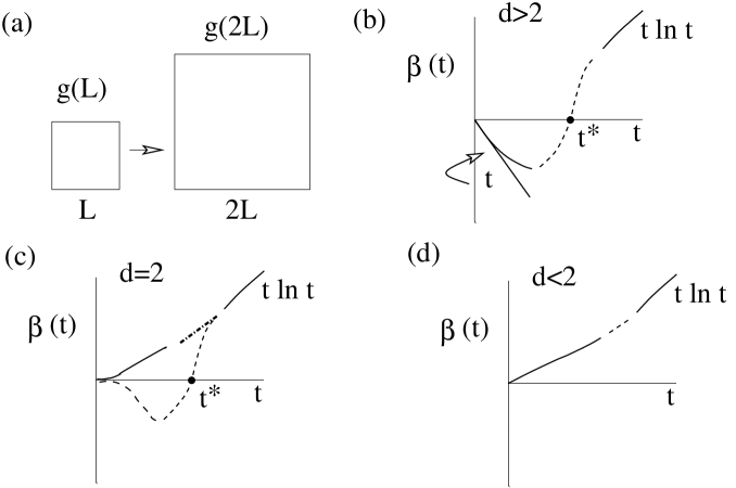
Figure 7: (a) Rescaling of a hypercubic box of side length $L$ to $2L$. The conductance ($>0$) goes from $g(L)$ to $g(2L)$. (b) The RG beta function $\beta(t)$, for $d>2$, goes from $\beta(t)\sim-t$ for small $t$ to positive values $\sim t\ln t,$ for large $t$. The dotted line is a possible extrapolation which necessarily goes through a zero, $\beta(t^{*})=0$. Here, $t^{*}$ is the RG fixed point. (c) For $d=2$, the $\beta$-function has zero slope at origin. Therefore, there are two possibilities, one with a zero and one without any. (d) For $d<2$, the slope at origin is positive, and there is unlikely to be any zero. The dashed lines are possible extrapolations

For a good conductor, we have $g(L)=\sigma_{0}L^{d-1}/L\sim L^{d-2}$ for a $d$-dimensional hypercube, because the conductance is proportional to the geometric factor $L^{d-1}/L$. Defining $t=1/(2\pi g)$, the scaling of $t$ can be expressed, in analogy with Eq. (3) and Eq. (46), as

$$\frac{\partial\ln t(L)}{\partial\ln L}=\epsilon\equiv(2-d),\quad{\rm or,}\quad L\frac{\partial t(L)}{\partial L}\equiv\beta(t)=\epsilon t,\quad({\rm small}\quad t).$$ (49)

This is the metallic regime.

On the other hand, if the states are localized in the strong disorder limit, i.e. all states are localized with a localization length $\xi$, then the conductance can be expressed as $g(L)=g_{0}\exp(-L/\xi)$. In this limit of $g\to 0$, and so we expect

$$L\frac{\partial g(L)}{\partial L}=g\;\ln g,\quad(g\to 0),\quad{\text{or,}}\quad L\frac{\partial t(L)}{\partial L}=t\;\ln t,\quad(t\to\infty).$$ (50)

By assuming that $\beta(t)$ depends only on $t$ (one parameter scaling, as for $u_{1}$ in Eq. (47), we combine Eqs. 49 and 50 as

$$\beta(t)=\left\{\begin{array}[]{ll}\epsilon\;t,&{\text{for}}\;t\to 0,\\ t\ln t,&{\text{for}}\;t\to\infty.\end{array}\right.$$ (53)

We see that $\beta(t)$ for $d=3$ goes from a negative value for small $t(>0)$ to a positive value, as shown schematically in Fig. 7. This means that there is a fixed point, $\beta(t^{*})=0$, where the parameter $t$ does not change with scale (“scale invariant”). It is straightforward to see that for any initial value $t_{0}<t^{*}$, the flow equation on integration to large $L$ takes $t\to 0$. Therefore on large scales the system behaves like a metal. In contrast for $t_{0}>t^{*}$ the flow goes to $t\to\infty$, an insulator. The difference in behaviour on the two sides of $t^{*}$ is ensured by $\beta^{\prime}(t^{*})\equiv d\beta(t)/dt|_{t^{*}}>0$. The unstable fixed point therefore represents a metal-insulator transition.

The power of the RG flow equation can be seen in several ways. If there is a fixed point with $\beta^{\prime}(t^{*})>0$,i.e. an unstable fixed point, it represents a transition point. Since no such fixed point exists for $d<2$, the flow always goes to the insulator region. In other words, all states will be localized for $d<2$. The linearized form around the fixed point is

$$L\frac{d\Delta t}{dL}\approx\beta^{\prime}(t^{*})\;\Delta t,\quad\Delta t\equiv t-t^{*}.$$ (54)

For small $\Delta_{0}\equiv|t_{0}-t^{*}|$, we may now find the length scale $\xi$ at which $\Delta t$ reaches a predetermined value $\tilde{\Delta}$. On integration, Eq. 54 gives (omitting the subscript of $t_{0}$)

$$\xi\sim|t-t^{*}|^{-\nu},\quad{\text{where}}\quad\nu=\frac{1}{\beta^{\prime}(t^{*})}\sim\frac{1}{|\epsilon|}.$$ (55)

In fact, Eq.55 is a very general prediction from RG for any critical point.

Problem 7.2:

The disorder problem involves a Hamiltonian with random matrix elements. Depending on the symmetry, the disorder problem can be classified in several groups with distinct $\beta$-function. For each of the following $\beta$-functions, determine the fixed point and $\nu$, and discuss the behaviour in two dimensions (for $\epsilon=0$).

1. For a class, called the orthogonal symmetry class, $\beta(t)=\epsilon t+2t^{2}+...$. Show that $t^{*}\approx|\epsilon|/2$ and $\nu=1/|\epsilon|,\epsilon<0$. In two dimensions, the flow is towards the insulator side, i.e. toa state where all states are localized.

2. For a class, called the unitary symmetry class, $\beta(t)=\epsilon t+2t^{3}+...$. Show that $t^{*}\approx\sqrt{|\epsilon|/2},\nu=1/(2|\epsilon|),\epsilon<0$. The two dimensional behaviour is same as the previous one, i.e., all states are localized.

3. There is a class called the symplectic class for which $\beta(t)=\epsilon t-t^{2}+...$. Show that at $d=2$, the behaviour is different from the above two, because now the flow is towards the metal side.

For more details see F. Evers and A. D. Mirlin, Rev.Mod.Phys. 80, 1355 (2008).

8 Multifractality

For completeness we mention another idea, namely multifractality.

In the quantum mechanics context, the difference between the wavefunctions of a bound state and an unbound state can be expressed in terms of the finite size behaviour. For a bound particle the size $L$ of the box is not important so long it is much larger than the width of the wavefunction. For an unbound state $\psi\sim L^{-d/2}$. These can be combined to write the behaviour of the finite size effect of the moments of the wavefunction as

$$\int d^{d}r\;|\psi(r)|^{2q}\sim\left\{\begin{array}[]{ll}L^{0},&{\rm(bound),}\\ L^{-d(q-1)},&{\rm(unbound),}\\ L^{-\tau_{q}},&{\rm(critical),}\end{array}\right.$$ (59)

where we introduced a new class called “critical” wave function for which $\tau_{q}$ is not linear in $q$ (note that the normalization condition requires $\tau_{1}=0$). For the bound state of width $\xi$, the insensitivity of the boundary, for $L\gg\xi$, is expressed by the power law $L^{0}$. For extended states, the moments are completely determined by the size of the box, with the exponent $d(q-1)$ following from dimensional analysis. In contrast, for the critical case, we find that for every moment a new length scale $\tau_{p}$ is required so that a critical wave function requires an infinite number of length scales to describe it. It is generally written as $\tau_{q}=d(q-1)+\Delta_{q}$, where $\Delta_{q}$ is the anomalous dimension. In other words, moments of $\psi$ explore different aspects of how the wave function is spread out in space.

For a large system, we may also revert to the box counting method of Sec. 4 as follows. For a wave function $\psi({\bf x})$, the probability $p(x)=|\psi(x)|^{2}$. So in the box method, instead of counting elements, we put an weight as

$$P_{q}=\sum_{i}\left(\int_{i\mathrm{th\ box}}d^{d}x\;|\psi({\bf x})|^{2}\right)^{q}=\sum_{i}\left(\int d^{d}xp(x)\right)^{q},$$

where the summation is over all the boxes of size $b$ covering the sample. There are $n=(L/b)^{d}$ number of boxes. Necessarily, $P_{1}=1,P_{0}=n$. In analogy with Eq. (59), we define

$$P_{q}\sim\left(\frac{L}{b}\right)^{-\tau_{q}}.$$ (60)

In such a situation, the quantity of interest is the fractal dimension of the set of points where $p=|\psi|^{2}\sim L^{-\alpha}$. Let the fractal dimension be given by $f(\alpha)$, i.e., the measure of the set of point with $|\psi|^{2}\sim L^{-\alpha}$ is $L^{f(\alpha)}$. This fractal dimension depends continuously on $\alpha$, justifying the name of “multifractal”. We just state here that the multifractal spectrum $f(\alpha)$ is related to $\tau_{q}$ by a Legendre transformation as

$$f(\alpha)=q\alpha-\tau_{q},\quad{\mathrm{where}}\quad\alpha=\partial\tau_{q}/\partial q.$$

The wavefunction at the localization transition mentioned in the Sec. 7.4 is an example of a multifractal wave function.

A tractable example of multifractal-like behaviour would be a power law decay of a wave function $\psi(r)$ which for large $r$ behaves as $\sim r^{-u}$, where $1/2<u<1$ In this situation, since $\int dr|\psi|^{2}$ is convergent, the wave function is normalizable, and therefore represents a bound state. The unusual nature of the bound state can be seen from the behaviour of the $q$th moment given by $\int dr\;r^{q}\;|\psi|^{2}$ which is divergent for $q>2u-1$. Note that $q$ is not necessarily an integer. A bound state with energy $E<0$ gives a length scale, $\xi\sim 1/\sqrt{|E|}$ which one may associate with the scale beyond which the wave function decays exponentially as $\exp(-r/\xi)$. In a sense this gives the width of the wave function and for most cases, like the square well potential or short range potentials, this scale is enough. However the situation we are considering corresponds to the case where for $\xi\to\infty$, the wave function goes over to the power law decay so that for $E$ very close to zero, there will be an intermediate range where the power law form is visible; for example a form like $\psi(r)\sim r^{-u}\;{\exp(-r/\xi)}$. A length scale to characterize the wavefunction in this intermediate range can be obtained from the moments as $\int dr\;r^{q}\;|\psi|^{2}\sim\int^{\xi}dr\;r^{q-2u}\sim\xi^{q-2u+1}$, for $\xi\to\infty$. In this limit the normalization constant is a number independent of $\xi$. We therefore find $l_{q}\sim\xi^{\tau_{q}}$ where $\tau_{q}=1-(2u-1)/q$, with an anomalous exponent $D_{q}=-(2u-1)/q$. This is not a carefully crafted example but occurs at the unbinding transition of a quantum particle in a potential $V(r)+a/r^{2}$ in three dimensions where $V(r)$ is a short range attractive potential. By tuning the short range potential, a zero energy bound state can be formed whose wave function decays in the power law fashion just mentioned.

9 Conclusion

In this chapter, we explored various definitions of dimensions, like the topological, the Hausdorff, the box or Minkowski, and the spectral dimensions by embedding the set in Euclidean space. When the Hausdorff and the box dimensions are the same, it is called the fractal dimension, and the set is called a fractal if this fractal dimension is different from the topological dimension. For Euclidean spaces, all these definitions give the same number, which, by construction, is a positive integer. However we have explicitly constructed various subsets of the Euclidean space whose dimensions are not integers. Further generalizations are made to study power law behaviour of various physical quantities in terms of renormalization group flow equations. The flow equations show the emergence of anomalous dimensions at certain special fixed points as opposed to engineering dimension determined by dimensional analysis. We also discussed how various physical properties are determined by various dimensions of the space.

Appendix A: Entropy and fractal dimension

We here establish the relation between entropy per spin of a chain of spins and the fractal dimension of the configuration space when mapped on to real numbers. The discussion is for a semi-infinite chain of spins which can be labeled by integrers, $1,2,...$.

Let us consider a chain of spins, each taking two values, $0$, and $1$. If all configurations are equally likely to occur, then the number of configurations for $N$ spins is $C_{N}=2^{N}$. The entropy per spin is therefore $s=k_{B}(\ln C_{N})/N=k_{B}\ln 2$. In general, the entropy per spin can be written as a derivative

$$s=k_{B}\;\;\frac{\ln C_{N+1}-\ln C_{N}}{(N+1)-N}=k_{B}\;\;\left.\frac{\partial\ln C_{N}}{\partial N}\right|_{N\to\infty},$$ (61)

where the last term is in the continuum limit.

Now we convert the strings of $0$ and $1$, $(s_{n}=0,1|n=1,...,N)$, to a real number by using base $m=3$ as

$$x=\sum_{n=1}^{N}\frac{2s_{n}}{m^{n}}.$$ (62)

As discussed in Sec. 4.1.4, for $N\to\infty$, $x$ forms the Cantor set. We chose $3$ because of our familiarity with the Cantor set, but $m=3$ is nothing special.

The fractal dimension of the subset of real numbers generated by all the spin configurations is given by the box dimension Eq. (15). As we go from $N$ to $N+1$ in the number of spins, we add a higher order term $2s_{N+1}/m^{N+1}$ in $x$. This is equivalent to changing the scale of the box size from $m^{-N}$ to $m^{-(N+1)}$, the latter being the finer scale. In other words, the “box”size has been changed by a scale factor $1/m$. The denominator of Eq. (15), with $b=1/m$, becomes $\ln m^{N+1}-\ln m^{N}=[(N+1)-N]\ln m$. The fractal dimension of the set is therefore

$$\framebox{$\displaystyle{d_{f}=\frac{1}{\ln m}\;\;\frac{\ln C_{N+1}-\ln C_{N}}{(N+1)-N}=\frac{1}{\ln m}\;\;\frac{s}{k_{B}},}$}$$

where we used Eq. (62). This establishes the connection between the entropy per spin and the fractal dimension of the set of real numbers equivalent to the configuration space.

For the Ising case, with $m=3$, we see $s\propto\ln 2/\ln 3=\log_{3}2$.

One may wonder, why we chose base $3$ ($m=3$). In general, for any choice of $m\geq 2$, the real numbers

$$x=\sum_{n=1}^{N}\frac{(m-1)s_{n}}{m^{n}},$$ (63)

form a subset of $[0,1]$. As the above result shows, we could have chosen any $m$ to get $s\propto\ln 2/\ln m$. The extra factor $\ln m$ could easily be absorbed in $k_{B}$ which is equivalent to changing the base of the logarithm. Our choice of $m=3$ is motivated by the fact that it is the smallest integer for uniqueness of the mapping, and our familiarity with the Cantor set.

Let us clarify the problem of mapping by taking the simplest situation of base $2$ ($m=2$). For any string we define $x=\sum_{i=1}^{\infty}s_{n}/2^{n}$, so that $x\in[0,1]$. Note that we get the whole interval. However, two strings $s_{1}s_{2}...s_{n}011111....$ gives the same value of $x$ as $s_{1}s_{2}...s_{n}1000000....$, like in traditional decimal system where $1.0=0.9999999...$. Therefore with base 2, we get a mapping from the binary strings to the real numbers $\in[0,1]$, but it is not unique; this is a many to one mapping. In contrast, with base $m\geq 3$, we get a unique one-to-one, onto and invertible mapping via Eq. (63). Nevertheless, as Prob 4.3 shows, the entropy can be related to the dimension of the space of points generated out of the strings with any base $m$. This includes $m=2$ with $\log_{2}2=1$, the dimension of the interval $[0,1]$!

In fields, like computing and telecommunication, $\log_{2}2=1$ is used as a unit (called Shannon) of information content of one bit (same as entropy).

The connection between entropy and fractal dimension for more general situations of spin chains are given as problems (Prob 4.1,4.2,4.3). Whether this connection can be extended to more general systems or general lattices remain to be seen.

Appendix B: Complex dimension: continuous and discrete Scaling

This appendix is technical in nature and may be skipped without loss of continuity.

The self similarity discussed so far is of geometric nature. This may be true for any property of a system. If a function $f(x)$ satisfies a relation $f(x)=b^{\mu}f(bx)$ then $f(x)$ is said to be scale invariant as $b$ may be viewed as a scale factor for the variable. If $b$ is arbitrary, then we may choose $bx=1$ to obtain $f(x)\sim x^{-\mu}$, a power law dependence on $x$. Thus power laws are synonymous to scale invariance - something one sees near critical points. Since $b$ is arbitrary, such a scale invariance is called a continuous scale invariance.

The scale invariance we saw for the geometric fractals are not continuous but discrete. Instead of choosing powers of $3$, suppose we choose some other $b,3^{n}<1/b<3^{n+1}$ as the scale factor for the Cantor set. For such a scale factor $x=1/b$, the number of pieces would remain the same, changing only when x matches with the correct scaling factor. It is then possible to write

$$C_{x}=Cx^{d_{\rm f}}F\left(\frac{\ln x}{\ln 3}\right),$$ (64)

where $F(z)$ is a periodic function of periodicity $1$. A Fourier expansion gives

$$F(z)=\sum_{n}(a_{n}e^{i2\pi nz}+a_{n}^{*}e^{-i2\pi nz}),$$ (65)

where $*$ denotes complex conjugation. On substitution in Eq. (64), one gets a simpler power law form with

$$d_{\rm f}^{\prime}=d_{\rm f}+i\frac{2\pi n}{\ln 3},\quad n\in\mathbb{Z},$$ (66)

a tower of complex dimensions. Restricting to the first mode, the oscillatory behaviour is of the form

$$C_{x}\sim x^{d_{\rm f}}\cos\left(2\pi\frac{\ln x}{\ln 3}\right).$$ (67)

Such an oscillatory behaviour for an arbitrary scale factor is a distinct signature of a discrete scale invariance. Whether these will have any important perceptible effect ultimately depends on the amplitudes $a_{n}$. In many situations, $|a_{n}|$ turns out to be extremely small compared to the nonoscillatory terms.

A notable example of a continuous scale invariance breaking into a discrete one is the Efimov effect in three body quantum mechanics or its classical analog in three stranded DNA.

B.1 Cantor string

Consider the complement of the Cantor set in the closed interval $[0,1]$. This is the set of disjoint lengths (open intervals) which add up to a length $1$, but still it is the whole line segment minus the set of points belonging to the Cantor set. A bounded open set of $\mathbb{R}$ is a fractal string, and the particular one we are discussing is the Cantor string. A poetic name is a one-dimensional drum with fractal boundary. A relevant question is ”Does one hear the shape of a drum?”

The fractal sting is described by the set of lengths $l_{j}$, $j=1,\infty$. For the Cantor string, these are $\frac{1}{3},\frac{1}{9},\frac{1}{9},...$, keeping track of the multiplicities (i.e., degeneracies), length $l_{j}$ occurring $m_{j}$ times. Let us define a zeta function

$$\zeta(s)=\sum_{j=1}^{\infty}\;m_{j}l_{j}^{s},$$ (68)

where $s$ is a complex number so that the series is convergent. For $s=1$, $\zeta(1)=1$, the length of the string. Since $l_{j}<1$, the series is definitely convergent for large positive real $s$. The minimum real value of $s$ for which it is convergent happens to be the fractal dimension of the boundary. On analytic continuation, one may define $\zeta(s)$ over the complex $s$-plane with singularities which are the complex dimensions of the boundary set. With an abuse of definition, the fractal dimension of the boundary is also called the dimension of the string.

For the Cantor string, $l_{j}=\frac{1}{3^{j}}$ with degeneracy $m_{j}=2^{j-1}$, so that

$$\zeta(s)=\sum_{j=1}\frac{1}{3^{s}}\;\left(\frac{2}{3^{s}}\right)^{j-1}=\frac{3^{-s}}{1-(2\times 3^{-s})},$$ (69)

which has poles at $3^{s}=2$, with $s$ given by Eq. (66).

Why should such a zeta function be useful? This becomes clear if we look upon Eq. (68) as a transformation for the weights $w_{j}$. Since $l_{j}<1$ and $l_{j}\to 0$ for $j\to\infty$, one may, in a very nonrigorous way, write the function as an integral

$$\zeta(s)=\int_{0}^{\infty}\ x^{-s}w(x)dx,$$ (70)

identifying the zeta function as the Mellin transformation of the weight function. A quantity of interest is the number of intervals of size less than ${\it x}$, $N(x)\sim\int_{0}^{x}w(x)dx$ for which the zeta functions are useful.

Appendix C: Spectral dimension for the Sierpinski Gasket

A scalar phonon problem on the Sierpinski gasket involves springs along the bonds of with equal masses at the sites but the restoring forces are added added disregarding the vectorial nature of the forces. This is equivalent to a resistor problem of finding the equivalent resistance between two sites if all the bonds are occupied by 1 Ohm resistors. By Kirchoff’s law, all the voltages are linearly added.

Figure 8: Notations for displacements or voltages in the scalar phonon problem. The capital letters will survive on elimination of the small letter variables from the equations.

With the notation $\lambda=m\omega^{2}/K$ where $m$ is the mass at the sites and the spring constant on the bonds, the equation of motion for say $x_{1}$ is

$$(4-\lambda)x_{1}-x_{2}-x_{3}=X_{2}+X_{3},$$ (71)

while the equations for $x_{2},x_{3}$ are obtained by appropriate permutations of the variables. Similarly for $z_{i}$’s. For the capital variables,

$$(4-\lambda)X_{1}=x_{2}+x_{3}+z_{2}+z_{3},$$ (72)

and so on. It is now straightforward to eliminate $x_{i}$’s and $z_{i}$’s to obtain an equation involving only the capital variables, as

$$(4=\lambda^{\prime})X_{1}=X_{2}+X_{3}+Z_{2}+Z_{3},\quad\lambda^{\prime}=\lambda(5-\lambda).$$ (73)

so that for small frequencies, $\lambda^{\prime}=5\lambda$.

Because of the change in the number of degrees of freedom under this scale change by $b=2$, the density of states should change as

$$\rho_{L/b}(\omega)=b^{-d_{\rm f}}\rho_{L}(\omega),$$ (74)

while the frequency itself may scale as

$$\omega(L)=b^{-\kappa}\omega(L/b).$$ (75)

Since the number of states remain invariant, i.e., $\rho_{L/b}(\omega^{\prime})d\omega^{\prime}=\rho_{L}(\omega)d\omega$, we have (using Eqs. (74,75))

$$\rho_{L/b}(\omega)=b^{-\kappa}\rho_{L}(\omega b^{-\kappa})=b^{-d_{\rm f}}\rho_{L}(\omega).$$ (76)

If we choose $\omega b^{-\kappa}=1$, then $\rho_{L}(\omega)=\omega^{d_{\rm f}/\kappa-1}$. The spectral dimension is therefore $d_{s}=d_{\rm f}/\kappa.$

From $\lambda^{\prime}\approx 5\lambda$, we have $z^{2\kappa}=5$, or, $\kappa=\frac{\ln 5}{2\ln 2}\neq 1$. Combining all, we find the spectral dimension of the Sierpinski Gasket to be

$$d_{s}=\left(\frac{\ln 3}{\ln 2}\right)\Big{/}\left(\frac{\ln 5}{2\ln 2}\right)=2\;\frac{\ln 3}{\ln 5},$$ (77)

using the fractal dimension, $d_{\rm f}=\ln 3/\ln 2$.

References

- [1] Benoit B. Mandelbrot, The Fractal Geometry of Nature (W. H. Freeman and Company,1982).
- [2] K. Falconer, Fractal Geometry: Mathematical Foundations and Applications, (Wiley, 3rd Edition, 2014)/
- [3] M. Lapidus and M. van Frankenhuijsen, Fractal Geometry, Complex Dimensions and Zeta Functions Geometry and Spectra of Fractal Strings, (Springer, 2013)
-
[4]
For a list of fractals with fractal dimensions, see
https://en.wikipedia.org/wiki/List_of_fractals_by_Hausdorff_dimension -
[5]
See Sec 9.14 of the online notes, J.Preskill,
http://www.theory.caltech.edu/preskill/ph219/topological.pdf - [6] S. Mukherji and S. M. Bhattacharjee, Phys. Rev. E 63, 051103 (2001).
- [7] S. M. Bhattacharjee, “Critical Phenomena: An Introduction from a modern perspective” in “Field theoretic methods in condensed matter physics” (TRiPS, Hindusthan Publising Agency, Pune, 2001). (cond-mat/0011011).
- [8] Y. Gefen, B. B. Mandelbrot, and A. Aharony, Phys. Rev. Letts 45, 855 (1980).
- [9] M. Janssen, Int. J. Mod. Phys. B 8, 943 (1994).
- [10] S. M. Bhattacharjee, “Entropy and perpetual computers”, Physics Teacher. 45, 12 (2003) (cond-mat/0310332).