A unified treatment of tidal disruption by Schwarzschild black holes

Abstract

Stars on orbits with pericenters sufficiently close to the supermassive black hole at the center of their host galaxy can be ripped apart by tidal stresses. Some of the resulting stellar debris becomes more tightly bound to the hole and can potentially produce an observable flare called a tidal-disruption event (TDE). We provide a self-consistent, unified treatment of TDEs by non-spinning (Schwarzschild) black holes, investigating several effects of general relativity including changes to the boundary in phase space that defines the loss-cone orbits on which stars are tidally disrupted or captured. TDE rates decrease rapidly at large black-hole masses due to direct stellar capture, but this effect is slightly countered by the widening of the loss cone due to the stronger tidal fields in general relativity. We provide a new mapping procedure that translates between Newtonian gravity and general relativity, allowing us to better compare predictions in both gravitational theories. Partial tidal disruptions in relativity will strip more material from the star and produce more tightly bound debris than in Newtonian gravity for a stellar orbit with the same angular momentum. However, for deep encounters leading to full disruption in both theories, the stronger tidal forces in relativity imply that the star is disrupted further from the black hole and that the debris is therefore less tightly bound, leading to a smaller peak fallback accretion rate. We also examine the capture of tidal debris by the horizon and the relativistic pericenter precession of tidal debris, finding that black holes of $10^{6}$ solar masses and above generate tidal debris precessing by $10^{\circ}$ or more per orbit.

I Introduction

Supermassive black holes (SBHs) with masses in the range from $10^{6}M_{\odot}\leq M_{\bullet}\leq 10^{10}M_{\odot}$ are found at the centers of most large galaxies Kormendy and Richstone (1995); Magorrian et al. (1998). Observations of quasars Schmidt (1963) and active galactic nuclei (AGN) have aided our understanding of these massive celestial objects, but these constitute only a small fraction Kauffmann et al. (2003) of all SBHs in the local universe, making it difficult to take a fully representative census of galactic nuclei. Studying quiescent SBHs, visible via their interactions with nearby stellar objects through the phenomena of tidal disruption events (TDEs) Rees (1988), would allow one to fill in this population gap, particularly for lower mass SBHs. Quiescent SBHs also have dynamical effects on neighboring stars and gas, but these can only be observed locally where the influence radius can be resolved.

TDEs occur when tidal forces due to a SBH’s gravitational field overcome an orbiting star’s self gravity, causing roughly half of the resulting debris to become more tightly bound to the SBH Rees (1988). This bound debris quickly forms a disk that is accreted by the SBH, releasing large amounts of energy in what is known as a tidal flare. Flares can be found in the optical van Velzen et al. (2011); Gezari et al. (2012); S. B. Cenko, et al. (2012a); I. Arcavi, et al. (2014); R. Chornock, et al. (2014); T. W.-S. Holoien, et al. (2014); J. Vinkó, et al. (2015), ultraviolet D. Stern, et al. (2004); S. Gezari, et al. (2006, 2008, 2009), soft X-ray Bade et al. (1996); Grupe et al. (1999); Donley et al. (2002a); P. Esquej, et al. (2008); Maksym et al. (2010); R. D. Saxton, et al. (2012), and hard X-ray J. S. Bloom, et al. (2011); D. N.Burrows, et al. (2011); S. B. Cenko, et al. (2012b) bands. A recent survey Donley et al. (2002b) discovered many candidate TDEs, showing rates consistent with those previously predicted by early models, resulting in an increased interest in TDEs in recent years.

Analysis of TDEs has been conducted under both Newtonian gravity Rees (1988); Magorrian and Tremaine (1999); Wang and Merritt (2004); Merritt (2013a); Cohn and Kulsrud (1978); Evans and Kochanek (1989); Lodato et al. (2009) and general relativity Luminet and Marck (1985); Laguna et al. (1993); Diener et al. (1997); Ivanov et al. (2003); Ivanov and Chernyakova (2006); Kesden (2012a, b); Sa̧dowski et al. (2016). In this paper, we provide a unified, self-consistent treatment of several aspects of the tidal-disruption process that are sensitive to general relativity. We explore how relativity changes the boundaries of the loss cone in phase space that determines TDE rates and the distribution of orbital elements for tidally disrupted stars. We then examine how relativity affects the distributions of the specific energy and angular momentum of the tidal debris and combine these results with recent hydrodynamical simulations to predict the rate at which this debris falls back onto the SBH to fuel a tidal flare Guillochon and Ramirez-Ruiz (2013).

We restrict ourselves in this paper to the Schwarzschild spacetime Schwarzschild (1916) corresponding to non-spinning SBHs. The spherical symmetry of the Schwarzschild metric implies that only the magnitudes of the orbital energy and angular momentum are needed to define the boundaries of the loss cone. However, in the Kerr spacetime Kerr (1963) of spinning SBHs, the orientation of the tidally disrupted star’s orbit with respect to the SBH’s equatorial plane affects the magnitude of the tidal stresses Ivanov and Chernyakova (2006). This creates a higher-dimensional parameter space, the analysis of which is beyond the scope of this paper. We will, however, provide some comments on SBH spin when relevant throughout the paper and lay the foundation for future work that will focus on incorporating spin dependence into our procedure.

The rest of this paper is structured as follows. Sec. II provides a brief overview of how loss-cone theory is used to calculate TDE rates in Newtonian gravity. Sec. III details how relativity changes the boundaries of the loss cone, allowing us to compare the TDE rates predicted in Newtonian gravity and general relativity. We then focus on trying to compare individual TDEs in the two gravitational theories, which introduces the somewhat subtle issue of which parameter to hold constant in these comparisons. We introduce a new procedure to map between Newtonian orbits and relativistic geodesics in Sec. IV that allows us to estimate how relativity would modify simulations performed in Newtonian gravity. In Sec. V, we use this mapping and loss-cone theory to predict distributions of physical quantities like the peak fallback accretion rate and amount of apsidal precession that affect observed TDE properties. A summary of our key results, their implications for TDE observations, and our plans to generalize to the Kerr spacetime are provided in Sec. VI.

II Newtonian loss-cone theory

We begin by providing a brief summary of Newtonian loss-cone theory Cohn and Kulsrud (1978); Magorrian and Tremaine (1999); Wang and Merritt (2004); Merritt (2013a). We define the tidal radius as

$$r_{t}\equiv\left(\frac{M_{\bullet}}{M_{\star}}\right)^{1/3}R_{\star}$$ (1)

where $M_{\bullet}$ is the mass of the SBH, $M_{\star}$ is the mass of the tidally disrupted star, and $R_{\star}$ is the stellar radius. This definition provides an order-of-magnitude estimate of the distance from the SBH at which tidal disruption occurs. Stars on parabolic orbits with pericenters equal to $r_{t}$ will have orbital angular momentum

$$L_{t}\equiv(2GM_{\bullet}r_{t})^{1/2}~{}.$$ (2)

Any star on an orbit with angular momentum $L\lesssim L_{t}$ will become tidally disrupted once it reaches a distance $r\sim r_{t}$ from the SBH. We can refine these estimates to account for stellar structure by introducing the parameter $\eta$ which measures the duration of the star’s pericenter passage relative to the hydrodynamical time of the star Press and Teukolsky (1977); Evans and Kochanek (1989). This parameter is a function of the polytropic index $\gamma$ of the star’s equation of state Chandrasekhar (1939). We may then define

$$r_{d} \equiv\eta^{2/3}r_{t}~{},$$ (3a)

$$L_{d} \equiv\eta^{1/3}L_{t}~{},$$ (3b)

the radial distance $r_{\rm d}$ and maximum orbital angular momentum $L_{\rm d}$ at which a star described by parameter $\eta$ is tidally disrupted. Throughout this paper, we use the value $\eta=0.382$ consistent with the threshold for full tidal disruption in Guillochon and Ramirez-Ruiz Guillochon and Ramirez-Ruiz (2013) for a Solar-type star with $\gamma=4/3$.

The TDE rate thus depends on the rate at which stars are driven onto such orbits, which are said to lie in the loss cone in phase space because the velocity vector lies in a cone about the radial direction. We assume that the stellar distributions in galactic centers are described by isothermal spheres with density profile

$$\rho(r)=\frac{\sigma^{2}}{2\pi Gr^{2}}$$ (4)

where $\sigma$ is the velocity dispersion given by the $M_{\bullet}-\sigma$ relation Gebhardt et al. (2000); Ferrarese and Merritt (2000). This is a reasonable approximation for galaxies with cusps in the surface brightness at their galactic centers Wang and Merritt (2004). We assume that loss-cone orbits are refilled by two-body non-resonant relaxation Cohn and Kulsrud (1978); Magorrian and Tremaine (1999); Wang and Merritt (2004); Merritt (2013a), in which case the differential flux $F$ of stars into the loss cone per unit dimensionless specific binding energy $\varepsilon^{*}\equiv\varepsilon/\sigma^{2}$, following the approach and notation of Merritt Merritt (2013b), is given by

$$F(\varepsilon^{*})=4\pi^{2}q(\varepsilon^{*})L^{2}_{d}\left[\int_{0}^{y_{d}}f(\varepsilon^{*},y)dy\right]~{}.$$ (5)

Here $q(\varepsilon^{*})$ is the orbital period divided by the time a star takes to diffuse across the loss cone, $y\equiv L^{2}/qL_{d}^{2}$ is a dimensionless angular-momentum variable, $y_{d}\equiv 1/q$, and $f(\varepsilon^{*},y)$ is the stellar phase-space density as a function of our dimensionless variables. For the stellar density profile of Eq. (4),

$$q(\varepsilon^{*})=\frac{32\pi^{2}}{3\sqrt{2}}\ln\Lambda\left(\frac{M_{\star}}{M_{\bullet}}\right)\frac{h(\varepsilon^{*})}{\psi^{*}(r_{d})-\varepsilon^{*}}\left(\frac{r_{d}}{r_{h}}\right)^{-2}$$ (6)

where $\ln\Lambda$ is the Coulomb logarithm Chandrasekhar (1943a, b, c), $\psi^{*}(r)\equiv-\Phi(r)/\sigma^{2}$ is the negative dimensionless potential energy, $r_{h}=GM_{\bullet}/\sigma^{2}$ is the influence radius Peebles (1972), and $h(\varepsilon^{*})$ (Eq. (6.78) of Merritt Merritt (2013b)) is a function derived from the isotropic distribution function consistent with our isothermal stellar density profile $\rho(r)$. We set $\Lambda=0.4M_{\bullet}/M_{\odot}$, appropriate for stars whose velocity distribution is consistent with the virial theorem Spitzer and Hart (1971); Wang and Merritt (2004).

The ratio $q$ helps provide intuition about how two-body relaxation feeds stars into SBHs. Portions of phase space with $q\ll 1$ are said to belong to the empty loss-cone (ELC) regime because diffusion is not efficient enough to repopulate loss-cone orbits on their dynamical timescale. Conversely, $q\gg 1$ corresponds to the full loss-cone (FLC) regime where diffusion is effective enough to keep orbits in these parts of phase space filled. SBHs with $M_{\bullet}\gtrsim 10^{7}\,M_{\odot}$ have $q\ll 1$ for $\varepsilon^{*}>1$ and thus belong primarily to the ELC regime, implying lower TDE rates despite their larger tidal radii Merritt (2013a). Approximately $30\%$ of TDEs occur in the FLC regime for the galaxy sample considered in Stone and Metzger Stone and Metzger (2016), where $\sim 50\%$ result in full rather than partial disruptions.

The integrand in Eq. (5) for the isotropic distribution function consistent with the isothermal density profile of Eq. (4) is given by

$$f(y)=f(y_{d})\left[1-\frac{2}{\sqrt{y_{d}}}\sum_{m=1}^{\infty}\frac{e^{-\gamma_{m}^{2}/4}}{\gamma_{m}}\frac{J_{0}(\gamma_{m}\sqrt{y})}{J_{1}(\gamma_{m}\sqrt{y_{d}})}\right]$$ (7)

where $J_{0}$ and $J_{1}$ are Bessel functions of the first kind and $\gamma_{m}$ is defined such that $\gamma_{m}\sqrt{y_{d}}$ is the $m$-th zero of $J_{0}$ Merritt (2013a). The flux of stars into the loss cone is then,

$$F(\varepsilon^{*})=4\pi^{2}L^{2}_{d}f(y_{d})\xi(q)$$ (8)

where $\xi(\varepsilon^{*})$ is defined to be $q$ times the integral in Eq. (5) and is well approximated by $\xi(q)\approx q/(q^{2}+q^{4})^{1/4}$. The total TDE rate is obtained by integrating over all binding energies,

$$\dot{N}=\int F(\varepsilon^{*})\,d\varepsilon^{*},$$ (9)

and depends implicitly on the SBH mass $M_{\bullet}$.

III Relativistic tidal forces

In Newtonian gravity, the tidal force acting on a fluid element of a star is simply the gravitational force in a frame freely falling with the star’s center of mass. In general relativity however, gravity affects particle motion through the curvature of spacetime. In this section, we review how tides arise in general relativity so that we can determine the value of the angular momentum $L_{d}$ that sets the boundary of the loss cone in this gravitational theory. We restrict our analysis in this paper to the Schwarzschild metric Schwarzschild (1916) describing non-spinning SBHs, which in Boyer-Lindquist coordinates Boyer and Lindquist (1967) is

$$ds^{2} =-\left(1-\frac{2M_{\bullet}}{r}\right)dt^{2}+\frac{r^{2}}{r^{2}-2M_{\bullet}}dr^{2}$$

$$\quad+r^{2}(d\theta^{2}+\sin^{2}\theta d\phi^{2}).$$ (10)

Massive test particles experiencing no non-gravitational forces travel on timelike geodesics $x^{\mu}(\tau)$ of this metric, the generalization of straight lines in flat space. We can choose to parameterize these geodesics by the proper time $\tau$. Particles traveling on these geodesics have conserved specific energy $E$ and specific angular momentum $L$ since the Schwarzschild metric is both time independent and spherically symmetric. Note that the specific energy

$$E\equiv-g_{\mu\nu}U^{\mu}\left(\frac{\partial}{\partial t}\right)^{\nu}=\left(1-\frac{2M_{\bullet}}{r}\right)\frac{dt}{d\tau}\,,$$ (11)

where

$$U^{\mu}=\frac{dx^{\mu}}{d\tau}=\left(\frac{dt}{d\tau},\frac{dr}{d\tau},\frac{d\theta}{d\tau},\frac{d\phi}{d\tau}\right)$$ (12)

is the 4-velocity, asymptotes to unity for particles at rest far from the SBH since it contains the rest-mass energy. We approximate $E=1$ for the orbits of tidally disrupted stars because the velocity dispersion $\sigma$ of their host galaxies is much less than the speed of light. This 4-velocity satisfies the geodesic equation

$$\frac{dU^{\mu}}{d\tau}+\Gamma^{\mu}_{\nu\alpha}U^{\nu}U^{\alpha}=0$$ (13)

where $\Gamma^{\mu}_{\nu\alpha}$ are the Christoffel symbols for the Schwarzschild metric. Note the resemblance to Newton’s second law $d\mathbf{v}/dt=0$ for force-free motion for vanishing Christoffel symbols as can be chosen for flat space.

In general relativity, tidal forces arise because of the tendency of parallel geodesics to deviate from each other in the presence of spacetime curvature. If two neighboring particles with 4-velocity $U^{\mu}$ are separated by an infinitesimal spacelike deviation 4-vector $X^{\beta}$, this deviation will evolve with proper time $\tau$ according to the geodesic deviation equation

$$\frac{d^{2}X^{\beta}}{d\tau^{2}} =U^{\mu}\nabla_{\mu}(U^{\alpha}\nabla_{\alpha}X^{\beta})=-R^{\beta}_{~{}\mu\alpha\nu}U^{\mu}X^{\alpha}U^{\nu}$$

$$=-C^{\beta}_{~{}\alpha}X^{\alpha}$$ (14)

where $\nabla_{\mu}$ are covariant derivatives, $d/d\tau\equiv U^{\alpha}\nabla_{\alpha}$ is the derivative with respect to the proper time, $R^{\beta}_{~{}\mu\alpha\nu}$ is the Riemann curvature tensor, and

$$C^{\beta}_{~{}\alpha}\equiv R^{\beta}_{~{}\mu\alpha\nu}U^{\mu}U^{\nu}$$ (15)

is the tidal tensor. In Newtonian gravity, a fluid element is tidally stripped from the surface of a star when the tidal force exerted by the SBH exceeds the force exerted on this fluid element by that star’s self gravity. If the star is non-degenerate like the Solar-type stars considered in this paper, we can approximate its self gravity as a Newtonian force even if general relativity is needed to describe the geodesics of the SBH. In this approximation, the fluid element is tidally stripped when the acceleration due to this self gravity is exceeded by the proper acceleration $d^{2}X/d\tau^{2}$ given by the geodesic deviation equation (14) Luminet and Marck (1983).

We can solve this equation more easily by transforming from the global Boyer-Lindquist coordinates given by Eq. (10) to local Fermi normal coordinates ($\tau,X^{(i)}$) valid in a neighborhood of spacetime about the center of mass of the star at an arbitrarily chosen proper time $\tau=0$ Manasse and Misner (1963). These coordinates define an orthonormal tetrad: the star’s 4-velocity provides the timelike 4-vector $\lambda^{\mu}_{~{}(0)}$, and three spacelike 4-vectors $\lambda^{\mu}_{~{}(i)}$ are chosen that are parallel transported along the geodesic. Spatial indices that run from 1 to 3 are denoted by Latin indices, unlike Greek indices that run from 0 to 3. All of the tensors appearing in the geodesic deviation equation can be projected into this basis:

$$U^{\mu} =\lambda^{\mu}_{~{}(0)}$$ (16a)

$$X^{\alpha} =X^{(i)}\lambda^{\alpha}_{~{}(i)}$$ (16b)

$$R^{\beta}_{~{}\mu\alpha\nu} =R^{(\gamma)}_{\quad(\delta)(\kappa)(\xi)}\lambda^{\beta}_{~{}(\gamma)}\lambda_{\mu}^{~{}(\delta)}\lambda_{\alpha}^{~{}(\kappa)}\lambda_{\nu}^{~{}(\xi)}$$ (16c)

$$C^{\beta}_{~{}\alpha} =C^{(i)}_{\quad(j)}\lambda^{\beta}_{~{}(i)}\lambda_{\alpha}^{~{}(j)}=R^{(i)}_{\quad(0)(j)(0)}\lambda^{\beta}_{~{}(i)}\lambda_{\alpha}^{~{}(j)}.$$ (16d)

The Boyer-Lindquist indices are raised and lowered by the Schwarzschild metric (10) while the Fermi normal coordinate indices in brackets are raised and lowered by the Lorentz metric $\eta_{(\mu)(\nu)}$. Note that the symmetry of the Riemann tensor implies that the tidal tensor is symmetric and only has spatial components in Fermi normal coordinates. Inserting Eq. (16) into (14) yields the geodesic deviation equation in Fermi normal coordinates

$$\frac{d^{2}X^{(i)}}{d\tau^{2}}=-C^{(i)}_{\quad(j)}X^{(j)}.$$ (17)

Because $C^{(i)}_{\quad(j)}$ is a real, symmetric $3\times 3$ tensor, it has 3 real eigenvalues which in Boyer-Lindquist coordinates are $M_{\bullet}/r^{3}$, $(1+3L^{2}/r^{2})M_{\bullet}/r^{3}$, and $-2(1+3L^{2}/2r^{2})M_{\bullet}/r^{3}$. The negative sign in Eq. (17) implies that the eigenvectors associated with the positive eigenvalues correspond to directions along which the star is compressed, while the eigenvector associated with the negative eigenvalue corresponds to the direction in which the star is stretched. Equating the magnitude of this negative eigenvalue times the stellar radius $R_{\star}$ with the acceleration $2M_{\star}/(\eta R_{\star})^{2}$ due to the star’s self gravity yields

$$\left(1+\frac{3L^{2}}{2r^{2}}\right)\frac{2M_{\bullet}R_{\star}}{r^{3}}=\frac{2M_{\star}}{(\eta R_{\star})^{2}}.$$ (18)

Combining this result with the relation

$$L^{2}=\frac{2M_{\bullet}r^{2}}{r-2M_{\bullet}},$$ (19)

between the orbital angular momentum $L$ and Boyer-Lindquist coordinate $r$ at pericenter provides two equations that can be solved for the the relativistic tidal radius $r_{d}$ and angular-momentum threshold $L_{d}$ for tidal disruption. Note that in the limit $r\gg 2M_{\bullet}$ these reduce to the Newtonian expressions of Eqs. (2) and (3).

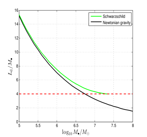
Figure 1: The angular-momentum threshold $L_{d}$ for tidal disruption as a function of SBH mass $M_{\bullet}$ in both Newtonian gravity (solid black) and general relativity (solid green). As the mass of the SBH increases, $L_{d}$ falls less steeply in relativity than in Newtonian gravity because of the stronger tidal forces. The horizontal red dashed line at $L_{\rm cap}=4M_{\bullet}$ indicates that direct capture by the event horizon occurs below this value, implying that SBHs with $M_{\bullet}>M_{\rm max}\simeq 10^{7.39}M_{\odot}$ cannot fully disrupt Solar-type stars.

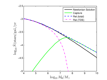
Figure 2: TDE rates in Newtonian gravity and general relativity as functions of SBH mass $M_{\bullet}$. The solid black curve shows the TDE rate in Newtonian gravity. In relativity, observable TDEs only result when the tides are strong enough to disrupt the star but the angular momentum is above the threshold $L_{\rm cap}$ for direct capture by the event horizon. The rate of such observable TDEs is given by the dot-dashed magenta curve, while the capture rate is shown by the solid green curve (the dashed blue curve shows the total of these two rates). Stronger tides in relativity slightly increase this total rate, but capture reduces the observed TDE rate in relativity below that of Newtonian gravity.

Fig. 1 shows how the angular-momentum threshold $L_{d}$ depends on SBH mass $M_{\bullet}$ in both Newtonian gravity and general relativity. All orbits with angular momentum $L$ below this threshold are considered to be inside the loss cone. The Newtonian tidal radius $r_{t}\propto M_{\bullet}^{1/3}$ according to Eq. (1), while the gravitational radius $r_{g}\equiv GM_{\bullet}/c^{2}$ scales linearly with SBH mass. This implies that relativistic effects become negligible for small SBH masses and the two curves in Fig. 1 converge towards the left edge of the plot. The fact that the term in brackets on the left-hand side of Eq. (18) is greater than unity implies that tidal forces are stronger in general relativity than in Newtonian gravity for orbits with the same angular momentum. This explains why the relativistic curve in Fig. 1 is above the Newtonian curve; stronger tides allow the SBH to disrupt stars at larger angular momentum $L_{d}$ in relativity.

Relativity also introduces the phenomena of stellar capture; stars on orbits with angular momentum less than $L_{\rm cap}=4M_{\bullet}$ will plunge directly into the event horizon leaving no debris to emit photons and generate an observable TDE. This angular-momentum threshold for direct capture, shown by the horizontal red dashed line in Fig. 1, grows linearly with SBH mass and eventually exceeds the threshold $L_{d}$ for tidal disruption at $M_{\bullet}=M_{\rm max}\simeq 10^{7.39}M_{\odot}$. This prevents observable TDEs by SBHs with masses above this value as shown by the intersection of the solid green and dashed red curves in Fig. 1.

Fig. 2 shows the rates for observable TDEs and direct capture predicted by Eq. (5) when two-body relaxation is responsible for refilling the loss cone. Relativity modifies the Newtonian prediction in two ways: (1) it changes the thresholds $r_{d}$ and $L_{d}$ in Eqs. (6) and (7) to the maximum of the two thresholds set by tidal disruption and direct capture, and (2) the limits of the integral in Eq. (5) must be modified. If $L_{\rm cap}<L_{d}$ ($M_{\bullet}<M_{\rm max}$), the integral must be decomposed into two parts: an integral from 0 to $y_{\rm cap}$ giving the capture rate and an integral from $y_{\rm cap}$ to $y_{d}$ giving the observable TDE rate. For $L_{\rm cap}\geq L_{d}$ ($M_{\bullet}\geq M_{\rm max}$), there are no observable TDEs and a single integral from 0 to $y_{\rm cap}$ gives the capture rate.

IV Comparing tidal disruption in Newtonian gravity and general relativity

Having introduced tidal disruption in Newtonian gravity and general relativity in Secs. II and III, we now seek to compare the predictions of the two theories. This point is more subtle than it might initially appear, as there is no unique way to map Keplerian orbits in Newtonian gravity to geodesics of the Schwarzschild metric in general relativity. In the limit that the pericenter $r\to\infty$, it is natural to map a geodesic to its identical Keplerian counterpart, but this limiting behavior is insufficient to fully specify the mapping. The appropriate mapping to use depends on the nature of the problem one is trying to solve. We consider in this section three distinct mappings that all possess the desired behavior in the Newtonian limit; these three mappings identify:

• orbits with equal pericenter coordinates $r$,

• orbits with equal angular momenta $L$,

• orbits on which a star experiences equal tidal forces at pericenter.

Mapping (1) is perhaps the most obvious choice and was used for the corrections to the orbital constants provided in Kesden Kesden (2012b). However, according to the Schwarzschild metric in Boyer-Lindquist coordinates given in Eq. (10), the physical significance of this mapping is that it identifies parabolic orbits such that the circular orbits in the two gravitational theories with the same pericenter $r$ would have the same circumference $2\pi r$. It is unclear why this choice of mapping would be particularly useful for analyzing the tidal disruption of stars on non-circular orbits.

Mapping (2) identifies orbits in the two theories with the same values of the gauge-invariant orbital angular momentum, defined for the Schwarzschild metric as

$$L\equiv g_{\mu\nu}U^{\mu}\left(\frac{\partial}{\partial\phi}\right)^{\nu}=r^{2}\frac{d\phi}{d\tau}$$ (20)

for equatorial orbits ($\theta=\pi/2$). This mapping seems like a useful choice, as TDE properties do depend on the orbital angular momentum as seen in the recent simulations of Guillochon and Ramirez-Ruiz Guillochon and Ramirez-Ruiz (2013). However, tides are stronger on Schwarzschild geodesics than on Keplerian orbits with the same value of $L$ as established in Sec. III, so it seems unlikely that TDEs on orbits in the two theories identified in this manner would have the same properties.

We conjecture that TDEs resulting from stars initially on orbits identified by mapping (3) will have similar properties because the stars were subjected to similar tidal forces. This conjecture is supported by the ”freezing” model of Lodato, King, and Pringle Lodato et al. (2009) which proposed that the orbital energy distribution of tidal debris is frozen in following an instantaneous tidal disruption of an unperturbed star. This model was used with reasonable success to describe the light curve of the TDE PS1-10jh Gezari et al. (2012). We will use this freezing assumption later in Sec. V to determine the appropriate relativistic correction to the energy distribution, but we will apply the correction at the disruption radius $r_{d}$ rather than pericenter. This is consistent with the analytic model of Stone, Sari, and Loeb Stone et al. (2013) and some hydrodynamical simulations of TDEs Hayasaki et al. (2013); Guillochon and Ramirez-Ruiz (2013) which showed that the spread in debris energy was largely independent of the orbital angular momentum $L$ for full disrupted stars.

To implement mapping (3), we must find the angular momentum $L_{N}$ of the orbit in Newtonian gravity that has the same peak tidal force as that experienced by a star on a Schwarzschild geodesic with angular momentum $L$ and pericenter $r$. We accomplish this by setting the magnitude of the negative eigenvalue of the tidal tensor $C^{(i)}_{\quad(j)}$ equal to its Newtonian limit for an orbit with angular momentum $L_{N}$:

$$\left(1+\frac{3L^{2}}{2r^{2}}\right)\frac{1}{r^{3}}=\left(\frac{2M_{\bullet}}{L_{N}^{2}}\right)^{3}.$$ (21)

This equation, combined with Eq. (19) relating the angular momentum $L$ to the pericenter $r$ in Boyer-Lindquist coordinates, can be solved to determine $L_{N}(L)$ for mapping (3).

Instead of using the angular momentum $L$ to identify orbits, the TDE literature often uses the penetration factor

$$\beta\equiv\frac{L_{t}^{2}}{L^{2}},$$ (22)

where $L_{t}$ is defined in Eq. (2). This choice is convenient because stars on orbits with $\beta\geq\beta_{d}\equiv L_{t}^{2}/L_{d}^{2}$ are tidally disrupted, where $\beta_{d}$ is of order unity. Our mapping $L_{N}(L)$ implies an equivalent mapping $\beta_{N}(\beta)$, where

$$\beta_{N}\equiv\frac{L_{t}^{2}}{L_{N}^{2}}=\left(\frac{r+M_{\bullet}}{r-2M_{\bullet}}\right)^{1/3}\frac{r_{t}}{r}$$ (23)

and $r$ is an implicit function of $L$ and hence $\beta$ through Eq. (19). We show this mapping for several values of the SBH mass $M_{\bullet}$ in Fig. 3. These mappings are undefined for $\beta>\beta_{\rm cap}\equiv L_{t}^{2}/L_{\rm cap}^{2}$ since such geodesics plunge directly into the event horizon and therefore do not have pericenters at which one can calculate the tidal force. The mappings $\beta_{N}(\beta)$ are above the diagonal and have positive curvature because tides are stronger in general relativity, requiring Newtonian orbits to have deeper penetration factors $\beta_{N}$ to match the tides on Schwarzschild geodesics at pericenter. The mapping for SBH mass $M_{\rm max}\simeq 10^{7.39}M_{\odot}$ terminates at $\beta_{N}(\beta_{\rm cap})=\beta_{N,d}=1.9$, precisely the threshold for the full disruption of Solar-type stars Guillochon and Ramirez-Ruiz (2013) seen in Fig. 1 for $L_{d}=L_{\rm cap}$.

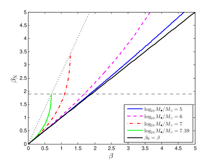
Figure 3: The mapping between Schwarzschild geodesics with penetration factor $\beta$ and orbits in Newtonian gravity with penetration factor $\beta_{N}$ on which stars experience the same tidal forces at pericenter. The solid blue, dashed magenta, dot-dashed red, and solid green curves show this mapping for SBHs with masses $M_{\bullet}/M_{\odot}$ of $10^{5}$, $10^{6}$, $10^{7}$, and $10^{7.39}$ respectively. The solid black diagonal $\beta_{N}=\beta$ shows the limit of these curves as $M_{\bullet}\to 0$, while the dotted black curve shows the relation $\beta_{N}(\beta_{\rm cap})$ beyond which these mappings are undefined. The horizontal black dashed line $\beta_{N,d}=1.9$ corresponds to full disruption in the hydrodynamical simulations of Guillochon and Ramirez-Ruiz Guillochon and Ramirez-Ruiz (2013).

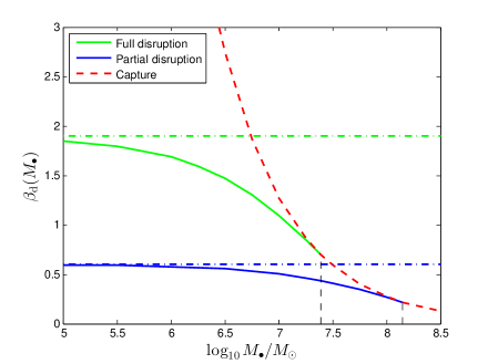
Figure 4: The minimum penetration factors $\beta_{d}$ and $\beta_{pd}$ for full and partial tidal disruption in general relativity as functions of SBH mass $M_{\bullet}$. The horizontal dot-dashed green and blue lines show the thresholds $\beta_{N,d}=1.9$ and $\beta_{N,pd}=0.6$ for full and partial disruption in Newtonian gravity Guillochon and Ramirez-Ruiz (2013). The solid green and blue curves show the values of $\beta_{d}$ for Schwarzschild geodesics on which stars experience the same tidal forces at pericenter. The intersections between these curves and the dashed red curve $\beta_{\rm cap}(M_{\bullet})$, marked by the vertical dashed lines, occur at the maximum SBH masses $M_{\rm max,FD}\simeq 10^{7.39}M_{\odot}$ and $M_{\rm max,PD}\simeq 10^{8.15}M_{\odot}$ capable of full and partial tidal disruption.

To further illustrate how relativity affects the minimum penetration factor $\beta_{d}$ for tidal disruption, we show its dependence on SBH mass $M_{\bullet}$ in Fig. 4 for both full and partial tidal disruptions. Newtonian hydrodynamical simulations Guillochon and Ramirez-Ruiz (2013) indicate that Solar-type stars are fully disrupted for $\beta_{N}>\beta_{N,d}=1.9$, while partial disruptions occur for $\beta_{N}>\beta_{N,pd}=0.6$. As $M_{\bullet}$ increases and $\beta_{d}$ approaches $\beta_{\rm cap}$, the $\beta_{d}$ curves fall increasingly below these Newtonian thresholds because of the stronger tides in general relativity. The values of $M_{\bullet}$ at which these curves intersect the $\beta_{\rm cap}$ curve are the maximum masses $M_{\rm max,FD}\simeq 10^{7.39}M_{\odot}$ and $M_{\rm max,PD}\simeq 10^{8.15}M_{\odot}$ capable of full and partial tidal disruption. These limits are consistent with recent work suggesting that observable TDEs by SBHs with masses above $10^{8}M_{\odot}$ result exclusively from giant stars MacLeod et al. (2012). Determinations of $M_{\rm max}$ that failed to account for the stronger relativistic tides, effectively using mapping (2) $\beta_{d}=\beta_{N,d}$ shown by the horizontal lines in Fig. 4, would underestimate $M_{\rm max}$ by a factor of $\sim 4.5$ for both full and partial disruptions. Future work will explore how SBH spin can push $M_{\rm max}$ to even higher values for stars on prograde orbits.

V Distributions of relativistic TDE properties

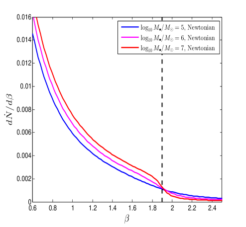
(a)

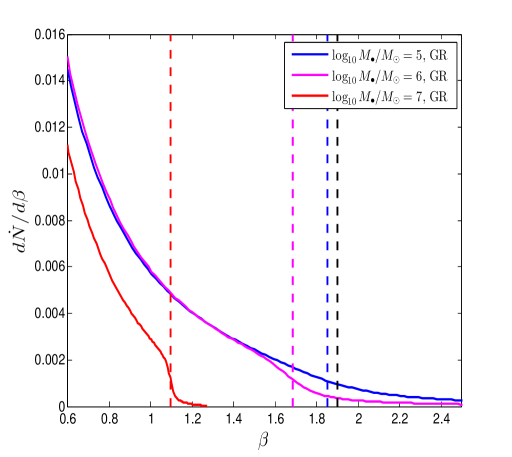
(b)

Figure 5: The differential TDE rate $d\dot{N}/d\beta$ per unit penetration factor for various SBH masses under Newtonian gravity (left) and relativity (right). The dashed black line in both panels shows the Newtonian threshold $\beta_{N,d}=1.9$ for full disruption, while the blue, magenta, and red dashed lines in the right panel show the thresholds $\beta_{d}$ in relativity defined through the the mapping $\beta_{N}(\beta_{d})=\beta_{N,d}$ between Newtonian orbits and Schwarzschild geodesics with the same tidal forces at pericenter.

In this section, we use concepts developed earlier in the paper to predict distributions of several quantities that affect the observed properties of TDEs. Guillochon and Ramirez-Ruiz Guillochon and Ramirez-Ruiz (2013) performed Newtonian hydrodynamical simulations to determine the peak accretion rate $\dot{M}_{\rm peak}$ at which tidal debris falls back on the SBH following a TDE and the delay $t_{\rm peak}$ between the tidal disruption and the time at which this peak accretion occurs. They then provided analytic fits to these quantities as functions of the Newtonian penetration factor $\beta_{N}$. Under the approximation that these quantities depend only on the peak tidal forces along each orbit, we use the inverse of the mapping $\beta_{N}(\beta)$ shown in Fig. 3 to derive fits to $\dot{M}_{\rm peak}$ and $t_{\rm peak}$ as functions of the relativistic penetration factor $\beta$ in the Schwarzschild spacetime. We then use the loss-cone theory discussed in Sec. II, modified by the relativistic corrections to the boundaries of the loss cone shown in Fig. 1, to predict the distributions of these quantities for different SBH masses.

In Subsec. V.1, we determine the differential TDE rate $d\dot{N}/d\beta$ per unit relativistic penetration factor $\beta$. In Subsec. V.2, we use this rate and our corrected fits $\dot{M}_{\rm peak}(\beta)$ and $t_{\rm peak}(\beta)$ to derive initial estimates for the differential TDE rates $d\dot{N}/d\dot{M}_{\rm peak}$ and $d\dot{N}/dt_{\rm peak}$ per unit peak fallback accretion rate and time delay respectively. These initial estimates do not account for an additional relativistic effect discussed in Kesden Kesden (2012b), that the gradient of the potential well that determines the width of debris energy distribution differs in general relativity and Newtonian gravity. We review this result and then derive revised estimates for $d\dot{N}/d\dot{M}_{\rm peak}$ and $d\dot{N}/dt_{\rm peak}$ in Subsec. V.3. The stellar debris produced following tidal disruption will also have a distribution of orbital angular momentum, but this often receives less attention in Newtonian gravity where the orbital periods that determine the fallback accretion rate depend on energy but not angular momentum. However, the distribution of orbital angular momentum can be very important when considering highly relativistic TDEs for which much of the debris can lose enough specific angular momentum to fall below the threshold for capture $L_{\rm cap}$ even if the initial star was above this threshold. We discuss this regime in Subsec. V.4 and show that this effect sharply limits the relativistic correction to the peak fallback accretion rate. Finally, in Subsec. V.5 we use our relativistically corrected loss-cone theory to determine the differential TDE rate $d\dot{N}/d\Delta\omega$ per unit relativistic shift in argument of pericenter, an important effect responsible for tidal stream crossings and the prompt circularization of debris Hayasaki et al. (2013); Dai et al. (2013); Guillochon et al. (2014); Guillochon and Ramirez-Ruiz (2015); Shiokawa et al. (2015).

V.1 Distribution of penetration factor $\beta$

We begin by calculating the differential TDE rate $d\dot{N}/d\beta$ in Newtonian gravity. The angular-momentum variable $y$ can be expressed in terms of the penetration factor $\beta$ as

$$y=\frac{L_{t}^{2}}{qL_{d}^{2}\beta}~{}.$$ (24)

This relation allows us to differentiate Eq. (5) with respect to $\beta$, which when combined with the distribution function in Eq. (7) yields

$$\frac{dF}{d\beta} =\left(\frac{2\pi L_{t}}{\beta}\right)^{2}f(y_{d})\times$$

$$\quad\left[1-2\sqrt{q}\sum_{m=1}^{\infty}\frac{e^{-\gamma_{m}^{2}/4}}{\gamma_{m}}\frac{J_{0}(\gamma_{m}L_{t}/L_{d}\sqrt{q\beta})}{J_{1}(\gamma_{m}/\sqrt{q})}\right]\,.$$ (25)

Integrating this expression with respect to the dimensionless specific binding energy $\varepsilon^{\ast}$ gives us the Newtonian differential TDE rate $d\dot{N}/d\beta$ shown in the left panel of Fig. 5 above. The total TDE rate is the area under this curve for $\beta_{N}>\beta_{N,d}$ which decreases with increasing SBH mass $M_{\bullet}$ consistent with the TDE rates seen in Fig. 2. The blue curve in the left panel of Fig. 5 extends smoothly beyond $\beta_{N,d}$ because much of the phase space beyond this value is still in the full loss-cone regime $q\gg 1$ for which $d\dot{N}/d\beta\propto\beta^{-1}$ Stone and Metzger (2016). However, as $M_{\bullet}$ increases towards $10^{7}M_{\odot}$, the differential TDE rate becomes exponentially suppressed for $\beta_{N}>\beta_{N,d}$ reflecting that much of the phase space beyond this point now lies in the empty loss-cone regime Stone and Metzger (2016).

Relativity introduces two changes into the calculation of the differential TDE rate $d\dot{N}/d\beta$: (1) the stronger tides increase the numerical value of $L_{d}$ from the Newtonian result given by the black curve in Fig. 1 to the relativistic result given by the green curve in this figure, and (2) capture by the event horizon cause the differential rate to fall discontinuously to zero for $\beta\geq\beta_{\rm cap}$. As most stars diffusing into the loss cone have apocenters near the influence radius $r_{h}=GM_{\bullet}/\sigma^{2}\gg r_{g}=GM_{\bullet}/c^{2}$ Frank and Rees (1976), the Newtonian treatment of stellar diffusion encapsulated in the ratio $q$ remains an accurate approximation. Both of the changes listed above leave signatures in the relativistic differential TDE rate $d\dot{N}/d\beta$ seen in the right panel of Fig. 5. The bends in these curves marking the threshold for full disruption in the empty loss-cone regime migrate to lower values of $\beta$ consistent with the SBH mass dependence of the mapping $\beta_{N}(\beta)$ shown in Fig. 3. The curves also end abruptly at $\beta_{\rm cap}$ as can be seen in the red curve corresponding to SBH mass $M_{\bullet}=10^{7}M_{\odot}$ for which $\beta_{\rm cap}\simeq 1.27$.

V.2 Distributions of peak fallback accretion rate $\dot{M}_{\rm peak}$ and time delay $t_{\rm peak}$

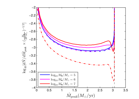
(a)

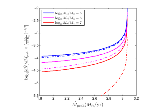
(b)

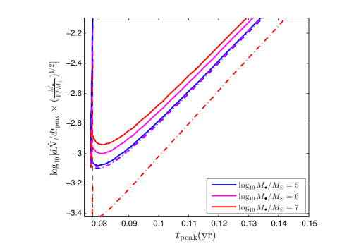
(c)

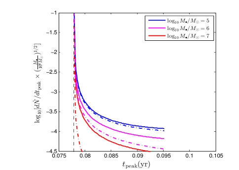
(d)

Figure 6: The differential TDE rates $d\dot{N}/d\dot{M}_{\rm peak}$ (top panels) and $d\dot{N}/dt_{\rm peak}$ (bottom panels) as functions of the peak fallback accretion rate $\dot{M}_{\rm peak}$ and time delay $t_{\rm peak}$ for partial (left panels) and full (right panels) disruptions. To clarify the presentation of relativistic effects, we have scaled out the explicit dependence on SBH mass $M_{\bullet}$ given on the right-hand side of Eq. (26). The solid (dot-dashed) curves show the differential TDE rates in Newtonian gravity (general relativity). The vertical dashed black lines indicate the values of $\dot{M}_{\rm peak}$ and time delay $t_{\rm peak}$ and the threshold $\beta_{N,d}=1.9$ of full disrpution.

Guillochon and Ramirez-Ruiz Guillochon and Ramirez-Ruiz (2013) performed a series of Newtonian hydrodynamical simulations at different penetration factors $\beta_{N}$ and used them to derive analytic fits to the peak fallback accretion rate $d\dot{M}_{\rm peak}/dt$ and time delay $t_{\rm peak}$ for Solar-type stars with polytropic index $\gamma=4/3$:

$$\dot{M}_{\rm peak} =A_{4/3}\left(\frac{M_{\bullet}}{10^{6}M_{\odot}}\right)^{-1/2},$$ (26a)

$$t_{\rm peak} =B_{4/3}\left(\frac{M_{\bullet}}{10^{6}M_{\odot}}\right)^{1/2},$$ (26b)

where,

$$A_{4/3} ={\rm exp}\left(\frac{27.3-27.5\beta_{N}+3.87\beta_{N}^{2}}{1-3.26\beta_{N}-1.39\beta_{N}^{2}}\right),$$ (27a)

$$B_{4/3} =\frac{-0.387+0.573\sqrt{\beta_{N}}-0.312\beta_{N}}{1-1.27\sqrt{\beta_{N}}-0.9\beta_{N}},$$ (27b)

and $0.6\leq\beta_{N}\leq 4.0$. Given these fits, the mapping $\beta_{N}(\beta)$ derived in Sec. IV, and the differential TDE rate $d\dot{N}/d\beta$ obtained in the previous subsection, we can calculate differential rates

$$\frac{d\dot{N}}{dX}=\frac{d\dot{N}}{d\beta}\left(\frac{d\beta_{N}}{d\beta}\frac{dX}{d\beta_{N}}\right)^{-1}$$ (28)

for $X\in\{\dot{M}_{\rm peak},t_{\rm peak}\}$. We show these differential TDE rates in Fig. 6 below. A complication arises from the fact that the dependence on penetration factor in Eq. (27) is not monotonic; $\dot{M}_{\rm peak}$ ($t_{\rm peak}$) increases (decreases) with $\beta_{N}$ until the threshold for full disruption $\beta_{N,d}$ is reached, then decreases (increases) for TDEs that penetrate more deeply into the SBH’s potential well. This $\beta_{N}$ dependence contradicts the naive predictions of freezing models which assume that the energy distribution of the tidal debris is frozen in at the disruption radius $r_{d}$, but does not fatally compromise our analyis. We address this complication by plotting the TDEs from partial ($\beta_{N}<\beta_{N,d}$) and full ($\beta_{N}>\beta_{N,d}$) disruptions separately in the left and right panels of Fig. 6. The differential rates diverge at the extremum $\beta_{N}=\beta_{N,d}$ shown by the vertical black dashed lines in these plots, but the total rates (areas under the curves) remain finite. We see that the stronger tides of relativity suppress the rates of both full and partial TDEs, particularly for SBH masses $M_{\bullet}\geq 10^{7}M_{\odot}$ for which portions of phase space with $\beta_{N}>\beta_{N,d}$ lie primarily in the empty loss-cone regime. This emptiness even reduces the rate of partial TDEs because of the sharper gradients driving stronger diffusion across the boundary as seen by the dip near the threshold in the top left panel of Fig. 6.

V.3 Relativistic correction to the debris energy distribution

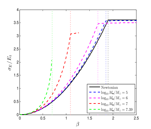
(a)

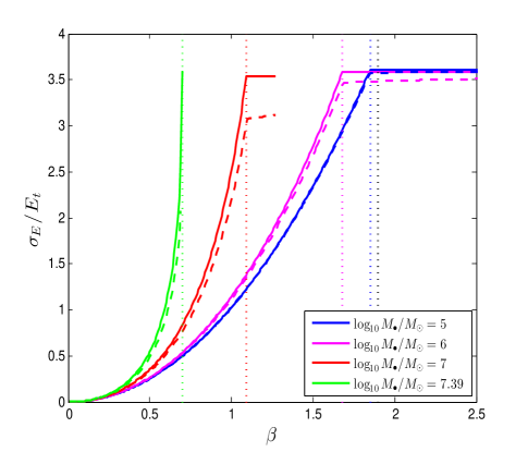
(b)

Figure 7: Dimensionless width $\sigma_{E}/E_{t}$ of the tidal debris energy distribution as a function of penetration factor $\beta$. The solid curves show the Newtonian predictions $\sigma_{E,\rm N}/E_{t}$, while the dashed blue, magenta, red, and green curves show the relativistic predictions $\sigma_{E,\rm GR}/E_{t}$ for $M_{\bullet}/M_{\odot}=10^{5}$, $10^{6}$, $10^{7}$, and $10^{7.39}$. The last value is $M_{\rm max}$, the most massive SBH capable of fully disrupting a Solar-type star. The vertical dotted lines show the thresholds $\beta_{d}$ for full disruption; each of the relativistic curves end at $\beta_{\rm cap}$. The single black curve in the left panel shows the Newtonian prediction in mapping (2) which is independent of SBH mass, while the three solid curves in the right panel show the Newtonian predictions for mapping (3).

The estimated differential TDE rates $d\dot{N}/d\dot{M}_{\rm peak}$ and $d\dot{N}/dt_{\rm peak}$ in the previous subsection accounted for relativistic corrections to the boundaries of the loss cone, but in the interest of a systematic exploration of relativistic effects we did not simulataneously include relativistic corrections to the energy distribution of the tidal debris. We turn our attention to this effect in this subsection.

A key approximation often used in the analysis of TDEs is that the tidal debris travels on ballistic trajectories following disruption, and that orbit circularization followed by viscous accretion occurs promptly after the bound debris falls back to pericenter Rees (1988); Evans and Kochanek (1989); Kochanek (1994). The fallback accretion rate onto the SBH, and thus its peak value $\dot{M}_{\rm peak}$ and the time $t_{\rm peak}$ between disruption and when this peak occurs, is determined by the distribution of orbital periods of the tidal debris, which is in turn set by the energy distribution through Kepler’s third law

$$\tau=2\pi\left(\frac{a^{3}}{M_{\bullet}}\right)^{1/2}=2\pi M_{\bullet}(2E)^{-3/2}\,.$$ (29)

This Newtonian relation remains an excellent approximation even for relativistic TDEs, because most of the debris is on highly eccentric orbits prior to circularization and spends most of its time near apocenter where Eq. (29) holds. However, if the tidal disruption itself occurs near pericenter where relativistic effects are strongest, Newtonian predictions for the specific binding energy $E$ entering into Eq. (29) may not be accurate. TDE simulations in general relativity Hayasaki et al. (2013); Cheng and Bogdanović (2014); Bonnerot et al. (2016); Shiokawa et al. (2015); Cheng and Evans (2013) naturally yield proper relativistic energy distributions, but our goal in this section is to study how relativistic corrections might alter the predictions of Newtonian simulations.

We addressed this issue in Kesden Kesden (2012b), where we found that for an undistorted star of radius $R_{\star}$, the width of the potential-energy distribution before disruption and thus the width of the debris energy distribution after disruption is given in general relativity by the expression

$$\sigma_{E,\rm GR}=|\lambda^{\alpha}_{~{}(i)}\nabla_{\alpha}E|R_{\star}=|g_{\beta\gamma}\lambda^{\beta}_{~{}(0)}\lambda^{\alpha}_{~{}(i)}\Gamma^{\gamma}_{\alpha t}|R_{\star},$$ (30)

where $g_{\beta\gamma}$ is the metric tensor, $\Gamma^{\gamma}_{\alpha t}$ are the Christoffel symbols, and $\lambda^{\beta}_{~{}(0)}$ and $\lambda^{\alpha}_{~{}(i)}$ are the orthonormal tetrad of basis 4-vectors determined by our choice of Fermi normal coordinates in Sec III. For $\beta<\beta_{d}$ corresponding to partial disruptions, tidal debris is assumed to be liberated at pericenter where the tidal forces are strongest. Evaluating Eq. (30) at pericenter for such orbits yields

$$\sigma_{E,\rm GR,PD} =\frac{M_{\bullet}R_{\star}}{r^{2}}\left(1-\frac{2M_{\bullet}}{r}\right)^{-1/2}$$

$$=E_{t}\left(\frac{r_{t}}{r}\right)^{2}\left(1-\frac{2M_{\bullet}}{r}\right)^{-1/2}.$$ (31)

The pericenter $r$ in Boyer-Lindquist coordinates can be expressed in terms of the angular momentum $L$ using Eq. (19),

$$E_{t}\equiv\frac{M_{\bullet}R_{\star}}{r_{t}^{2}}=\left(\frac{M_{\bullet}}{M_{\star}}\right)^{1/3}\frac{M_{\star}}{R_{\star}}=\left(\frac{M_{\bullet}}{M_{\star}}\right)^{1/3}E_{\star}$$ (32)

is an order-of-magnitude estimate for the width of this energy distribution, and $E_{\star}\equiv M_{\star}/R_{\star}$ is a similar estimate for the specific self-binding energy of the star. The mass hierarchy $M_{\star}\ll M_{\bullet}$ implies that $E_{\star}\ll E_{t}$, supporting the assumption of freezing models that the relative velocities of fluid elements at the time of disruption can be neglected when determining the debris energy distribution.

In trying to compare this relativistic result to Newtonian predictions, we encounter the same issue of choosing a mapping between the two gravitational theories that we addressed in Sec. IV. Mapping (1), which was used in Kesden Kesden (2012b), compared Eq. (31) to Newtonian orbits with the same pericenter coordinate and found

$$\sigma_{E,\rm N,PD(1)}=\frac{M_{\bullet}R_{\star}}{r^{2}}=E_{t}\left(\frac{r_{t}}{r}\right)^{2}.$$ (33)

Dividing Eq. (31) by Eq. (33) yields a peak correction of $\sqrt{2}$ for $r=4M_{\bullet}$, the minimum pericenter for an orbit that avoids direct capture by the horizon. As argued in Sec. IV however, this mapping is a somewhat unnatural way to identify orbits in the two theories.

Mapping (2) compared Schwarzschild geodesics to Newtonian orbits with the same angular momentum $L$ (and hence penetration factor $\beta=L_{t}^{2}/L^{2}$). For this choice, the width of the Newtonian energy distribution is

$$\sigma_{E,\rm N,PD(2)}=\frac{M_{\bullet}R_{\star}}{r_{L}^{2}}=E_{t}\left(\frac{2M_{\bullet}}{L^{2}}\right)^{2}=\beta^{2}E_{t}~{},$$ (34)

where $r_{L}$ is the pericenter of a Newtonian orbit with angular momentum $L$. Freezing models posit that the energy distribution is frozen in for $\beta>\beta_{N,d}$, implying that $\sigma_{E,\rm N,FD(2)}=\beta_{N,d}^{2}E_{t}$ for full disruptions in mapping (2). Although there is no nice analytic expression for the widths $\sigma_{E,\rm GR,FD}$ for full disruption in general relativity, they can be calculated numerically using Eq. (30). We show the widths of these distributions in mapping (2) for both partial and full disruptions in the left panel of Fig. 7. We see that for partial disruptions $\beta<\beta_{d}$, the energy distribution is broader in relativity than Newtonian gravity. The ratio $\sigma_{E,\rm GR}/\sigma_{E,\rm N(2)}$ reaches a maximum value of $4\sqrt{2}$ at $M_{\rm max}$, even larger than the peak correction in mapping (1). However, the weaker tides in Newtonian gravity imply that stars can reach larger penetration factors $\beta_{N,d}>\beta_{d}$ before being fully disrupted. SBHs with masses $M_{\bullet}\simeq 10^{6}M_{\odot}$ can have deeply penetrating encounters $\beta_{d}<\beta<\beta_{\rm cap}$ where the star still manages to avoid direct capture. For such penetration factors, the relativistic prediction can fall below that in Newtonian gravity as can be seen near the right edge of the left panel of Fig. 7. It is interesting to note that the relativistic predictions retain some mild $\beta$ dependence for full disruptions $\beta>\beta_{d}$, unlike in Newtonian freezing models. This is because the tidal tensor $C^{(i)}_{\quad(j)}$ and energy width $\sigma_{E,\rm GR}$ are velocity-dependent in relativity, even if evaluated at the fixed tidal acceleration $2M_{\star}/(\eta R_{\star})^{2}$ set by the star’s self gravity.

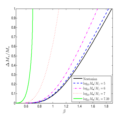
Figure 8: The fraction $\Delta M_{\star}/M_{\star}$ of the stellar mass lost in partial disruptions as a function of penetration factor $\beta$. The solid black curve shows a fit to Newtonian simulations Guillochon and Ramirez-Ruiz (2013), while the blue, magenta, red, and green curves show the corresponding relativistic predictions made using our mapping $\beta_{N}(\beta)$ for SBH masses $M_{\bullet}/M_{\odot}=10^{5}$, $10^{6}$, $10^{7}$, and $M_{\rm max}/M_{\odot}\simeq 10^{7.39}$.

Mapping (3) solves the problem of stars being fully disrupted at different values of $\beta$ in the two theories by identifying the Schwarzschild geodesic with penetration factor $\beta$ with the Newtonian orbit with penetration factor $\beta_{N}(\beta)$ on which a star experiences the same peak tidal force at pericenter as shown in Fig. 3. In this case, the width of the energy distribution for partial disruptions is

$$\sigma_{E,\rm N,PD(3)}=\frac{M_{\bullet}R_{\star}}{r_{F}^{2}}=\beta_{N}^{2}(\beta)E_{t}=\frac{M_{\bullet}R_{\star}}{r^{2}}\left(\frac{r+M_{\bullet}}{r-2M_{\bullet}}\right)^{2/3}~{},$$ (35)

where $r_{F}$ is the pericenter of a Newtonian orbit with penetration factor $\beta_{N}(\beta)$ and $r$ as previously is the pericenter in Boyer-Lindquist coordinates of a Schwarzschild geodesic with penetration factor $\beta$. This width again freezes out at $\sigma_{E,\rm N,FD(3)}=\beta_{N,d}^{2}E_{t}$ for full disruptions as in mapping (2), but these full disruptions now occur for $\beta>\beta_{d}$ as in general relativity. We show $\sigma_{E,\rm GR}$ and $\sigma_{E,\rm N(3)}$ as functions of penetration factor $\beta$ in the right panel of Fig. 7. We see that full disruption occurs at $\beta_{d}$ in both theories with this mapping, but that for a given penetration factor $\beta$, the relativistic predictions $\sigma_{E,\rm GR}$ are now below the Newtonian predictions $\sigma_{E,\rm N(3)}$. The deeper penetration needed for tidal disruption in Newtonian gravity leads to steeper potential gradients and thus broader tidal debris energy distributions. The ratio $\sigma_{E,\rm GR}/\sigma_{E,\rm N(3)}$ reaches a minimum value of $(128/625)^{1/6}\simeq 0.768$ at $M_{\rm max}$. The Newtonian orbit mapped to the Schwarzschild geodesic with $L_{\rm cap}=4M_{\bullet}$ has $L_{N}=(1024/5)^{1/6}M_{\bullet}\simeq 2.43M_{\bullet}<L_{\rm cap}$, but this is not a problem in principle since Newtonian point masses have no horizons to capture stars.

Which of the three expressions given by Eqs. (33), (34), (35) is the ”right” one to use when comparing TDEs in Newtonian gravity with those in general relativity? The answer to this question depends on which of the three mappings discussed in Sec. IV you are using to relate orbits in the two theories. If you want to compare orbits with the same angular momentum $L$, Eq. (34) provides the width of the tidal energy distribution for a Newtonian orbit with the same penetration factor $\beta$, leading to more tightly bound debris in relativity for partial disruptions as seen in the left panel of Fig. 7. However, this choice implies that different fractions of the stellar mass are stripped away by tides as seen in Fig. 8. More material is lost by the partially disrupted star in relativity, further enhancing the fallback accretion rate in addition to the more tightly bound material falling back more quickly. For $\beta_{d}<\beta<\beta_{d,N}$, full disruptions occur in general relativity but not Newtonian gravity, while for $\beta>\beta_{d,N}$ stars are fully disrupted in both theories but the tidal debris is more tightly bound in Newtonian gravity.

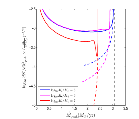
(a)

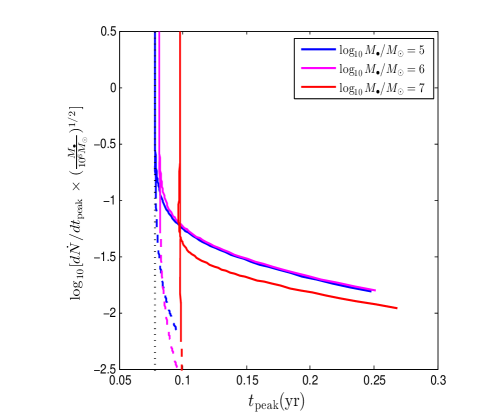
(b)

Figure 9: The differential TDE rates $d\dot{N}/d\dot{M}_{\rm peak}$ (left panel) and $d\dot{N}/dt_{\rm peak}$ (right panel) as functions of the peak fallback accretion rate $\dot{M}_{\rm peak}$ and time delay $t_{\rm peak}$ between disruption and when this peak is reached. The blue, magenta, and red curves show SBH masses $M_{\bullet}/M_{\odot}=10^{5}$, $10^{6}$, and $10^{7}$. The solid curves show partial disruptions while the dashed curves show full disruptions. The vertical black dotted lines show the values in Newtonian gravity at the threshold $\beta_{N,d}$ for full disruption.

If you are instead trying use Newtonian TDE simulations like those in Guillochon and Ramirez-Ruiz Guillochon and Ramirez-Ruiz (2013) to predict what this process might be like in relativity, you should use mapping (3) to relate orbits experiencing the same peak tidal forces and thus the same amount of mass loss by partially disrupted stars. Eq. (35) should be used to determine the relativistic correction $\sigma_{E,\rm GR}/\sigma_{E,\rm N(3)}$ as shown in the right panel of Fig. 7. We use this correction to predict the peak fallback accretion rate and time delay

$$\dot{M}_{\rm peak}(\beta) =\left(\frac{\sigma_{E,\rm GR}}{\sigma_{E,\rm N(3)}}\right)^{3/2}\times\dot{M}_{\rm peak}[\beta_{N}(\beta)]\,,$$ (36a)

$$t_{\rm peak}(\beta) =\left(\frac{\sigma_{E,\rm GR}}{\sigma_{E,\rm N(3)}}\right)^{-3/2}\times t_{\rm peak}[\beta_{N}(\beta)]\,,$$ (36b)

in general relativity, where the exponent of 3/2 follows from the energy dependence in Kepler’s third law (29). We show the corrected differential TDE rates $d\dot{N}/d\dot{M}_{\rm peak}$ and $d\dot{N}/dt_{\rm peak}$ in Fig. 9. We see that the peak fallback accretion rates $\dot{M}_{\rm peak}$ have been reduced below their Newtonian values by $\sim 20\%$ for a $10^{7}M_{\odot}$ SBH, consistent with Eq. (36) and the ratios of the curves shown in the right panel of Fig. 7. The time delays $t_{\rm peak}$ show a corresponding increase. Fig. 9 conveys the qualitative message of this subsection: the stronger tides in general relativity allow SBHs to tidally disrupt stars at lower penetration factors $\beta$ leading to less tightly bound debris and lower fallback accretion rates.

V.4 Capture of tidal debris by the event horizon

In this subsection, we focus on an issue that was only briefly addressed in Kesden Kesden (2012b): tidal debris can be captured by the event horizon of an SBH even if the disrupted star is not initially on a capture orbit. In general relativity, the tidal debris will have a distribution of specific angular momentum $L$ with a width given by

$$\sigma_{L,{\rm GR}}=|\lambda^{\alpha}_{~{}(i)}\nabla_{\alpha}L|R_{\star}=|g_{\beta\gamma}\lambda^{\beta}_{~{}(0)}\lambda^{\alpha}_{~{}(i)}\Gamma^{\gamma}_{\alpha\phi}|R_{\star}$$ (37)

analogous to Eq. (30) giving the width of the specific energy distribution. This width is set at pericenter $r$ for partial disruptions, allowing us to evaluate Eq. (37) as

$$\sigma_{L,{\rm GR,PD}}=R_{\star}\left(\frac{2M_{\bullet}}{r}\right)^{1/2}=L_{t}\left(\frac{M_{\star}}{M_{\bullet}}\right)^{1/3}\left(\frac{r_{t}}{r}\right)^{1/2}.$$ (38)

The mass hierarchy $M_{\star}\ll M_{\bullet}$ between the star and SBH implies that $\sigma_{L,{\rm GR}}\ll L_{t}$ and thus that it is usually a good approximation to assume that the specific angular momentum of the tidal debris is equal to that of the initial star. This contrasts with the debris energy distribution for which $E_{t}\gg\sigma^{2}$ implying that the tidal debris is much more tightly bound to the SBH than the initial star. However, for highly relativistic TDEs, the small amount of specific angular momentum lost in the disruption process may be enough for some of the tidal debris to be captured by the horizon. We examine this possibility by defining the dimensionless parameter

$$f_{L}\equiv\frac{L+\Delta L-L_{\rm cap}}{|\Delta L|}=\frac{L-4M_{\bullet}}{|\Delta L|}-1\,,$$ (39)

where $L$ is the specific angular momentum of the initial star, $\Delta L<0$ is the change in specific angular momentum of a fluid element in the disruption process, and $L_{\rm cap}=4M_{\bullet}$ is the specific angular momentum threshold for direct capture by the horizon. An element of the tidal debris with $f_{L}<0$ will be captured by the SBH, and $f_{L}=-1$ is the minimum value of this parameter for a star that is not originally on a capture orbit ($L>L_{\rm cap}$).

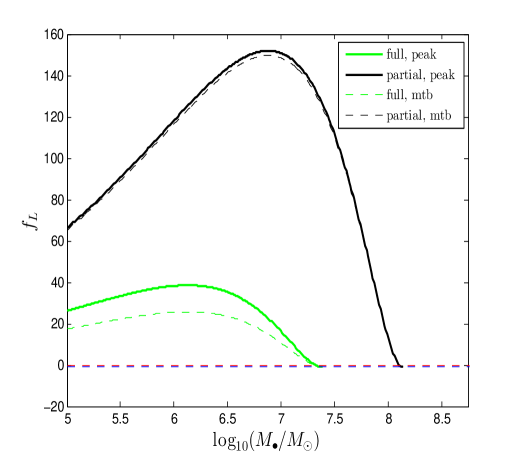
(a)

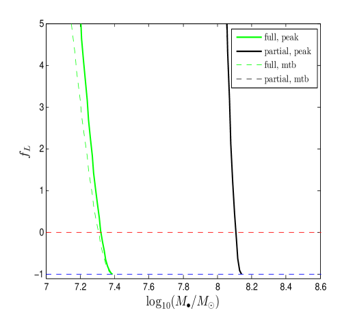
(b)

Figure 10: The parameter $f_{L}\equiv(L+\Delta L-L_{\rm cap})/|\Delta L|$, a measure of whether tidal debris is at risk of direct capture by the event horizon, as a function of SBH mass $M_{\bullet}$. The green (black) curves correspond to stars at the thresholds $\beta=\beta_{d}~{}(\beta_{pd})$ for full (partial) disruptions. The solid curves correspond to elements of the tidal debris that fall back onto the SBH when fallback accretion peaks, while the dashed curves represent the most tightly bound (mtb) elements (first to fall back). The red (blue) horizontal dashed lines show the reference values $f_{L}=0~{}(-1)$.

We need an estimate for $\Delta L$ to evaluate our new parameter $f_{L}$. In the freezing model, an element of the tidal debris located at $X^{(i)}$ in Fermi normal coordinates at tidal disruption has its specific energy and angular momentum changed by an amount

$$\Delta E \equiv X^{(i)}r_{E(i)}=X^{(i)}\lambda^{\alpha}_{~{}(i)}\nabla_{\alpha}E\,,$$ (40a)

$$\Delta L \equiv X^{(i)}r_{L(i)}=X^{(i)}\lambda^{\alpha}_{~{}(i)}\nabla_{\alpha}L\,,$$ (40b)

in the tidal-disruption process. The element of the star that will become the most tightly bound element of the tidal debris will have $X^{(i)}$ of magnitude $R_{\star}$ anti-aligned with $r_{E(i)}$, leading to the specific binding energy $\sigma_{E,{\rm GR}}$ given by Eq. (30). The element of the star that loses the most angular momentum in the tidal-disruption process will have $X^{(i)}$ of magnitude $R_{\star}$ anti-aligned with $r_{L(i)}$ and have its angular momentum reduced by an amount $\sigma_{L,{\rm GR}}$ given by Eq. (37). If $r_{E(i)}$ and $r_{L(i)}$ are parallel to each other (as at pericenter in Newtonian gravity, where both point in the radial direction), the same element of the tidal debris will be both the mostly tightly bound (the first to fall back onto the SBH) and have lost the most angular momentum (and thus be at greatest risk for direct capture). We will assume this to be true, as it is exactly true in general relativity at pericenter and a good approximation for those fluid elements with $f_{L}\lesssim 1$ most at risk of direct capture. Under this assumption, TDEs for which $f_{L}\leq 0$ for $\Delta L=-\sigma_{L,{\rm GR}}$ in Eq. (39) will have suppressed fallback accretion rates and greater delays between disruption and the beginning of emission because direct capture will have removed the most tightly bound debris. Furthermore, if $r_{E(i)}$ and $r_{L(i)}$ are parallel, there is a one-to-one relationship

$$\Delta L=\frac{|r_{L(i)}|}{|r_{E(i)}|}E$$ (41)

between the specific binding energy $E$ of an element of tidal debris and the specific angular momentum $\Delta L$ it loses during tidal disruption. If we use Kepler’s third law (29) to relate the time delay $t_{\rm peak}$ to the specific binding energy $E_{\rm peak}$ of debris accreted at that time, we can use Eq. (41) to estimate $\Delta L$ and thus $f_{L}$ for such debris. When this estimate of $f_{L}$ becomes negative, all of the debris accreted before the fallback accretion rate reaches its peak will be captured by the horizon.

We show $f_{L}$ for both peak and most tightly bound fluid elements as a function of SBH mass $M_{\bullet}$ in Fig. 10, for stars with penetration factors $\beta_{d}$ and $\beta_{pd}$ corresponding to the thresholds for full disruption and nonzero partial disruption. For the most tightly bound elements with $\Delta L=-\sigma_{L,{\rm GR}}$, Eq. (39) yields

$$f_{L}=\left(\frac{M_{\bullet}}{M_{\star}}\right)^{1/3}\left(\frac{r}{r_{t}}\right)^{1/2}\left[\frac{1}{\sqrt{\beta}}-\left(\frac{M_{\bullet}}{M_{\star}}\right)^{1/3}\sqrt{8E_{\star}}\right]-1\,.$$ (42)

For $M_{\star}\ll M_{\bullet}$, the term in the square brackets goes to $\beta^{-1/2}$ and $f_{L}\propto M_{\bullet}^{1/3}$, however as $M_{\bullet}$ increases this term decreases and ultimately reaches zero ($f_{L}=-1$) for $L=L_{\rm cap}$ when the entire star is directly captured. This increase then subsequent decrease in $f_{L}$ as a function of $M_{\bullet}$ is seen in the left panel of Fig. 10 indicating that tidal debris is safe from direct capture for all but the most massive SBHs. Only when $M_{\bullet}$ is within $\sim 20\%$ of $M_{\rm max}$ does the direct capture of tidal debris become significant as seen in the right panel of Fig. 10. Although such events constitute only a small fraction of the total TDE rate, they are the TDEs subject to the most extreme relativistic effects such as the pericenter precession that will be considered in the next subsection.

V.5 Relativistic pericenter precession

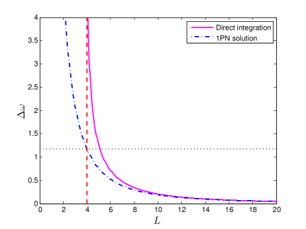
Figure 11: Precession of argument of pericenter $\Delta\omega$ (in units of radians) as a function of the specific angular momentum $L$. The solid magenta and dot-dashed blue curves show the exact precession and its 1PN approximation, respectively. The vertical dashed red line show the capture threshold $L_{\rm cap}=4M_{\bullet}$ and the horizontal dotted line shows the 1PN prediction for precession at this threshold.

Early work on TDEs assumed that tidal debris would promptly circularize after falling back to pericenter Rees (1988), but Newtonian hydrodynamical simulations demonstrated that energy dissipation at pericenter was inefficient for $M_{\star}\ll M_{\bullet}$ Guillochon et al. (2014). Early analytic work suggested that relativistic pericenter precession might promote orbit circularization, because this precession would lead to steam crossings at which the inelastic collisions of tidal elements would transform orbital kinetic energy into heat that could be subsequently radiated away. This suggestion was later supported by relativistic TDE simulations in which such precession was indeed shown to generate tidal stream crossings Hayasaki et al. (2013); Dai et al. (2013); Guillochon and Ramirez-Ruiz (2015); Shiokawa et al. (2015).

The angular coordinate $\omega$ specifying the location of pericenter with respect to a reference axis in the orbital plane is known as the argument of pericenter. In Newtonian gravity, the argument of pericenter is a constant of motion, but this is not true for Schwarzschild geodesics of the metric (10) in Boyer-Lindquist coordinates. At lowest post-Newtonian (PN) order, the argument of pericenter changes by an amount

$$\Delta\omega_{\rm 1PN}=6\pi\left(\frac{M_{\bullet}}{L}\right)^{2}=6\pi\beta\left(\frac{M_{\bullet}}{M_{\star}}\right)^{2/3}E_{\star}~{}.$$ (43)

This PN approximation breaks down for $L\gtrsim L_{\rm cap}$ for which pericenter precession must be integrated numerically along Schwarzschild geodesics,

$$\Delta\omega_{S}=2\int_{r}^{\infty}\frac{\dot{\phi}}{|\dot{r}|}dr^{\prime}-2\pi\,,$$ (44)

where

$$\dot{r} =\pm\left\{\frac{2M_{\bullet}}{r}\left[1+\left(\frac{L}{r}\right)^{2}\right]-\left(\frac{L}{r}\right)^{2}\right\}$$ (45a)

$$\dot{\phi} =\left(\frac{L}{r}\right)^{2}$$ (45b)

are the first-order derivatives of the Boyer-Lindquist coordinates $r$ and $\phi$ with respect to proper time $\tau$. The lower limit of the integral in Eq. (44) is the pericenter $r$ which depends implicitly on $L$ and hence $\beta$ through Eq. (19). We can set the upper limit of this integral to $\infty$ since we assume the tidally disrupted stars are initially on nearly parabolic orbits and the tidal debris remains highly eccentric. Eq. (38) also indicates that we can approximate the specific angular momentum of the tidal debris as equal to that of the initial star. We plot $\Delta\omega_{\rm 1PN}$ and $\Delta\omega_{S}$ in Fig. 11, which shows that pericenter precession diverges at $L=L_{\rm cap}$ guaranteeing a tidal stream crossing and perhaps subsequent orbit circularization of the tidal debris.

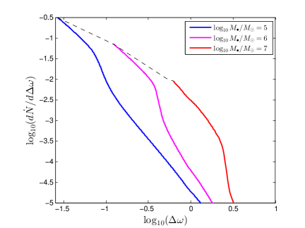
Figure 12: The differential TDE rate $d\dot{N}/d\Delta\omega$ as a function of the precession of the argument of pericenter $\Delta\omega$. The solid blue, magenta, and red curves show this distribution for SBH masses $M_{\bullet}/M_{\odot}=10^{5}$, $10^{6}$, and $10^{7}$, respectively. The dashed black curve connects the lower limit of each rate curve corresponding to the threshold $\beta_{pd}$ of partial disruption.

Given that $\Delta\omega_{S}$ is a function of $\beta$, we can use the differential TDE rate $d\dot{N}/d\beta$ derived in Sec. V.1 and shown in the right panel of Fig. 5 to derive the differential TDE rate $d\dot{N}/d\Delta\omega$. We show this rate in Fig. 12 for several SBH masses $M_{\bullet}$. As expected from Eq. (43), TDEs by more massive SBHs have greater amount of pericenter precession suggesting that relativistic orbit circularization might be more effective in such events. Further investigation of this possibility requires a criterion for orbit circularization that we hope to explore in future work.

VI Discussion

In this paper, we have systematically compared tidal disruption by Schwarzschild black holes in general relativity and point masses in Newtonian gravity. Differences between the two theories have potentially observable consequences for both TDE rates and the properties of individual events:

(1) Tidal forces are stronger in general relativity than Newtonian gravity for orbits with the same penetration factor $\beta\equiv L_{t}^{2}/L^{2}$. This implies that the loss cone within which stars are tidally disrupted is larger in general relativity: $L_{d}>L_{d,N}\Longrightarrow\beta_{d}<\beta_{d,N}$. Partially disrupted stars with $\beta<\beta_{d}$ will lose more material in relativity than Newtonian gravity, and stars with $\beta_{d}<\beta<\beta_{d,N}$ will be fully disrupted in relativity but not Newtonian gravity.

(2) The width $\sigma_{E}$ of the energy distribution of tidal debris is larger in general relativity than Newtonian gravity for orbits with the same penetration factor $\beta$. This implies that stars will not only lose more material in partial disruptions in relativity, but this material will become more tightly bound to the SBH and fall back to pericenter more quickly, leading to a higher peak luminosity if the radiative efficiency is fixed. However, stars that are fully disrupted in both theories ($\beta>\beta_{d,N}$) will be disrupted higher in the potential well in relativity than Newtonian gravity because of the stronger tides. This implies that the tidal debris will be less tightly bound despite the relativistic correction and therefore that the peak fallback accretion rate is lower in relativity than Newtonian gravity.

(3) Black holes have event horizons in general relativity that allow them to directly capture stars. This reduces the TDE rate in relativity compared to Newtonian gravity, since tidal debris captured by the horizon cannot emit photons detectable by observers. As the threshold $L_{\rm cap}$ for direct capture increases more steeply with SBH mass than the thresholds $L_{d}$ and $L_{pd}$ for full and partial disruptions, SBHs with masses greater than $M_{\rm max,d}=2.5\times 10^{7}M_{\odot}$ and $M_{\rm max,pd}=1.4\times 10^{8}M_{\odot}$ will no longer be capable of full and partial disruption, respectively. These limits would have been underestimated by a factor of $\sim 4.5$ without accounting for the stronger tides in relativity.

(4) Event horizons can capture a portion of the tidal debris in general relativity, even if the tidally disrupted star is not initially on a capture orbit. Tidal debris loses both energy and angular momentum during tidal disruption. If the specific angular momentum of the initial star was already close to the capture threshold, this additional loss can cause some of the debris to plunge directly into the horizon. This captured debris is the most tightly bound part of the tidal stream for $\beta\lesssim\beta_{d}$, so its capture suppresses the early portions of the TDE light curve assuming the luminosity traces the fallback accretion rate.

(5) Tidal streams precess in general relativity, potentially leading to inelastic collisions between parts of the stream that allow energy to be dissipated and debris orbits to circularize. At lowest PN order, this precession scales as $M_{\bullet}^{2/3}$ at the threshold $\beta_{d}$ for full disruption, but it increases more steeply with SBH mass as $\beta_{d}$ approaches the threshold for direct capture $\beta_{\rm cap}$.

In future work, we plan to explore how SBH spin affects all five of these relativistic effects. By breaking the spherical symmetry of the spacetime, SBH spin increases the parameter space to include spin magnitude, orbital inclination, and argument of pericenter. As the tidal forces along geodesics depend on all these parameters, the diffusion equation determining the rate at which stars enter the loss cone will likely need to be solved numerically to account for the higher-dimensional boundary conditions. Qualitatively, we expect TDE rates to be biased in favor of stars on retrograde orbits for moderate SBH masses, but this bias should switch towards stars on prograde orbits as the retrograde threshold for disruption falls below that for direct capture. Both of these biases will tend to spin down the SBH, as a larger fraction of the stellar material will be accreted in each case from retrograde orbits. TDEs from stars on prograde orbits however will be more luminous because of the more tightly bound prograde innermost stable circular orbits, leading to a potential observational bias in favor of prograde TDEs.

SBH spin also affects relativistic precession. At 1.5PN order, spin-dependent pericenter precession opposes (supports) the 1PN pericenter precession considered in this paper on prograde (retrograde) orbits Merritt (2013b), imposing a further bias in favor of retrograde TDEs if such precession is required for orbit circularization. SBH spin induces precession of the longitude of ascending node which can cause tidal streams to precess out of their initial orbital planes, inhibiting stream crossings and delaying orbit circularization Guillochon and Ramirez-Ruiz (2015); Hayasaki et al. (2016). Spin-dependent solutions of stellar diffusion into the loss cone will allow us to calculate the fraction of TDEs experiencing such delays between disruption and peak fallback accretion. By providing a unified treatment of TDEs in the Schwarzschild spacetime, this paper performs an important service in its own right and establishes a beachhead for attacking the more ambitious problem of tidal disruption by spinning Kerr black holes.

References

- Kormendy and Richstone (1995) J. Kormendy and D. Richstone, Ann. Rev. Astron. Astrophys. 33, 581 (1995).
- Magorrian et al. (1998) J. Magorrian, S. Tremaine, D. Richstone, R. Bender, G. Bower, A. Dressler, S. M. Faber, K. Gebhardt, R. Green, C. Grillmair, J. Kormendy, and T. Lauer, Astron. J. 115, 2285 (1998).
- Schmidt (1963) M. Schmidt, Nature 197, 1040 (1963).
- Kauffmann et al. (2003) G. Kauffmann, T. M. Heckman, C. Tremonti, J. Brinchmann, S. Charlot, S. D. M. White, S. E. Ridgway, J. Brinkmann, M. Fukugita, P. B. Hall, Ž. Ivezić, G. T. Richards, and D. P. Schneider, Mon. Not. R. Astron. Soc. 346, 1055 (2003), astro-ph/0304239 .
- Rees (1988) M. J. Rees, Nature 333, 523 (1988).
- van Velzen et al. (2011) S. van Velzen, G. R. Farrar, S. Gezari, N. Morrell, D. Zaritsky, L. Östman, M. Smith, J. Gelfand, and A. J. Drake, Astrophys. J. 741, 73 (2011), arXiv:1009.1627 [astro-ph.CO] .
- Gezari et al. (2012) S. Gezari, R. Chornock, A. Rest, M. E. Huber, K. Forster, E. Berger, P. J. Challis, J. D. Neill, D. C. Martin, T. Heckman, A. Lawrence, C. Norman, G. Narayan, R. J. Foley, G. H. Marion, D. Scolnic, L. Chomiuk, A. Soderberg, K. Smith, R. P. Kirshner, A. G. Riess, S. J. Smartt, C. W. Stubbs, J. L. Tonry, W. M. Wood-Vasey, W. S. Burgett, K. C. Chambers, T. Grav, J. N. Heasley, N. Kaiser, R.-P. Kudritzki, E. A. Magnier, J. S. Morgan, and P. A. Price, Nature 485, 217 (2012), arXiv:1205.0252 [astro-ph.CO] .
- S. B. Cenko, et al. (2012a) S. B. Cenko, et al., Mon. Not. R. Astron. Soc. 420, 2684 (2012a), arXiv:1103.0779 [astro-ph.HE] .
- I. Arcavi, et al. (2014) I. Arcavi, et al., Astrophys. J. 793, 38 (2014), arXiv:1405.1415 [astro-ph.HE] .
- R. Chornock, et al. (2014) R. Chornock, et al., Astrophys. J. 780, 44 (2014), arXiv:1309.3009 .
- T. W.-S. Holoien, et al. (2014) T. W.-S. Holoien, et al., Mon. Not. R. Astron. Soc. 445, 3263 (2014), arXiv:1405.1417 .
- J. Vinkó, et al. (2015) J. Vinkó, et al., Astrophys. J. 798, 12 (2015), arXiv:1410.6014 [astro-ph.HE] .
- D. Stern, et al. (2004) D. Stern, et al., Astrophys. J. 612, 690 (2004), astro-ph/0405482 .
- S. Gezari, et al. (2006) S. Gezari, et al., Astrophys. J. Lett. 653, L25 (2006), astro-ph/0612069 .
- S. Gezari, et al. (2008) S. Gezari, et al., Astrophys. J. 676, 944-969 (2008), arXiv:0712.4149 .
- S. Gezari, et al. (2009) S. Gezari, et al., Astrophys. J. 698, 1367 (2009), arXiv:0904.1596 [astro-ph.CO] .
- Bade et al. (1996) N. Bade, S. Komossa, and M. Dahlem, Astron. Astrophys. 309, L35 (1996).
- Grupe et al. (1999) D. Grupe, H.-C. Thomas, and K. M. Leighly, Astron. Astrophys. 350, L31 (1999), astro-ph/9909101 .
- Donley et al. (2002a) J. L. Donley, W. N. Brandt, M. Eracleous, and T. Boller, Astron. J. 124, 1308 (2002a), astro-ph/0206291 .
- P. Esquej, et al. (2008) P. Esquej, et al., Astron. Astrophys. 489, 543 (2008), arXiv:0807.4452 .
- Maksym et al. (2010) W. P. Maksym, M. P. Ulmer, and M. Eracleous, Astrophys. J. 722, 1035 (2010), arXiv:1008.4140 [astro-ph.HE] .
- R. D. Saxton, et al. (2012) R. D. Saxton, et al., Astron. Astrophys. 541, A106 (2012), arXiv:1202.5900 .
- J. S. Bloom, et al. (2011) J. S. Bloom, et al., Science 333, 203 (2011), arXiv:1104.3257 [astro-ph.HE] .
- D. N.Burrows, et al. (2011) D. N.Burrows, et al., Nature 476, 421 (2011), arXiv:1104.4787 [astro-ph.HE] .
- S. B. Cenko, et al. (2012b) S. B. Cenko, et al., Astrophys. J. 753, 77 (2012b), arXiv:1107.5307 [astro-ph.HE] .
- Donley et al. (2002b) J. L. Donley, W. N. Brandt, M. Eracleous, and T. Boller, Astron. J. 124, 1308 (2002b), astro-ph/0206291 .
- Magorrian and Tremaine (1999) J. Magorrian and S. Tremaine, Mon. Not. R. Astron. Soc. 309, 447 (1999), astro-ph/9902032 .
- Wang and Merritt (2004) J. Wang and D. Merritt, Astrophys. J. 600, 149 (2004), astro-ph/0305493 .
- Merritt (2013a) D. Merritt, Classiacl and Quantum Gravity 30, 244005 (2013a), arXiv:1307.3268 .
- Cohn and Kulsrud (1978) H. Cohn and R. M. Kulsrud, Astrophys. J. 226, 1087 (1978).
- Evans and Kochanek (1989) C. R. Evans and C. S. Kochanek, Astrophys. J. Lett. 346, L13 (1989).
- Lodato et al. (2009) G. Lodato, A. R. King, and J. E. Pringle, Astrophys. J. 392, 332 (2009).
- Luminet and Marck (1985) J.-P. Luminet and J.-A. Marck, Mon. Not. R. Astron. Soc. 212, 57 (1985).
- Laguna et al. (1993) P. Laguna, W. A. Miller, W. H. Zurek, and M. B. Davies, Astrophys. J. Lett. 410, L83 (1993).
- Diener et al. (1997) P. Diener, V. P. Frolov, A. M. Khokhlov, I. D. Novikov, and C. J. Pethick, Astrophys. J. 479, 164 (1997).
- Ivanov et al. (2003) P. B. Ivanov, M. A. Chernyakova, and I. D. Novikov, Mon. Not. R. Astron. Soc. 338, 147 (2003), astro-ph/0205065 .
- Ivanov and Chernyakova (2006) P. B. Ivanov and M. A. Chernyakova, Astron. Astrophys. 448, 843 (2006), astro-ph/0509853 .
- Kesden (2012a) M. Kesden, Phys. Rev. D 85, 024037 (2012a), arXiv:1109.6329 [astro-ph.CO] .
- Kesden (2012b) M. Kesden, Phys. Rev. D 86, 064026 (2012b), arXiv:1207.6401 .
- Sa̧dowski et al. (2016) A. Sa̧dowski, E. Tejeda, E. Gafton, S. Rosswog, and D. Abarca, Mon. Not. R. Astron. Soc. 458, 4250 (2016), arXiv:1512.04865 [astro-ph.HE] .