Node Embedding via Word Embedding for Network Community Discovery

Abstract

Neural node embeddings have recently emerged as a powerful representation for supervised learning tasks involving graph-structured data. We leverage this recent advance to develop a novel algorithm for unsupervised community discovery in graphs. Through extensive experimental studies on simulated and real-world data, we demonstrate that the proposed approach consistently improves over the current state-of-the-art. Specifically, our approach empirically attains the information-theoretic limits for community recovery under the benchmark Stochastic Block Models for graph generation and exhibits better stability and accuracy over both Spectral Clustering and Acyclic Belief Propagation in the community recovery limits.

I Introduction

Learning a representation for nodes in a graph, also known as node embedding, has been an important tool for extracting features that can be used in machine learning problems involving graph-structured data [1, 2, 3, 4]. Perhaps the most widely adopted node embedding is the one based on the eigendecomposition of the adjacency matrix or the graph Laplacian [2, 5, 6]. Recent advances in word embeddings for natural language processing such as [7] has inspired the development of analogous embeddings for nodes in graphs [8, 3]. These so-called “neural” node embeddings have been applied to a number of supervised learning problems such us link prediction and node classification and demonstrated state-of-the-art performance [8, 3, 4].

In contrast to applications to supervised learning problems in graphs, in this work we leverage the neural embedding framework to develop an algorithm for the unsupervised community discovery problem in graphs [9, 10, 11, 12]. The key idea is straightforward: learn node embeddings such that vectors of similar nodes are close to each other in the latent embedding space. Then, the problem of discovering communities in a graph can be solved by finding clusters in the embedding space.

We focus on non-overlapping communities and validate the performance of the new approach through a comprehensive set of experiments on both synthetic and real-world data. Results demonstrate that the performance of the new method is consistently superior to those of spectral methods across a wide range of graph sparsity levels. In fact, we find that the proposed algorithm can empirically attain the information-theoretic phase transition thresholds for exact and weak recovery of communities under the Stochastic Block Model (SBM) [13, 14, 11, 15]. SBM is a canonical probabilistic model for random graphs with latent structure and has been widely used for empirical validation and theoretical analysis of community detection algorithms [16, 17, 10, 9]. In particular, when compared to the best known algorithms based on Acyclic Belief Propagation (ABP) that can provably detect communities at the information-theoretic limits [15, 11, 14], our approach has consistently better accuracy. In addition, we find that ABP is very sensitive to random initialization and exhibits high variability. In contrast, our approach is stable to both random initialization and a wide range of algorithm parameter settings.

Our implementation and scripts to recreate all the results in this paper are available at https://github.com/cy93lin/SBM_node_embedding

II Related Works

The community detection problem has been extensively studied in the literature [9, 10, 12, 18], [19]. It has important applications in various real-world networks that are encountered in sociology, biology, signal processing, statistics and computer science. One way to systematically evaluate the performance of a community detection algorithm and establish theoretical guarantees is to consider a generative model for graphs with a latent community structure. The most widely-adopted model is the classic Stochastic Block Model. SBM was first proposed in [16, 20, 21] as a canonical model for studying community structure in networks and various community detection algorithms based on it have been proposed, e.g., [22, 5, 23, 24]. Among these approaches, algorithms that are based on the graph spectrum and semidefinite programming relaxations of suitable graph-cut objectives have been extensively studied [23, 24]. In particular, the phase transition behavior of spectral graph clustering for a generative model that includes SBM as a special case has also been established recently [25]. Graph-statistics based algorithms such as modularity optimization and their connection to Bayesian models on graphs have also been studied [26]. Only very recently have the information-theoretic limits for community recovery under the general SBM model been established [13, 11, 15]. In [11, 15], a belief-propagation based algorithm has been shown to asymptotically detect the latent communities in an SBM and achieve the information-theoretic limits. It has also been shown that graph spectrum based algorithms cannot achieve the information-theoretic limits for recovering communities in SBM models [11].

The use of a neural-network to embed natural language words into Euclidean space was made popular by the famous “word2vec” algorithm [7, 27]. In these works, each word in a vocabulary is represented as a low-dimensional vector in Euclidean space. These representations are learned in an unsupervised fashion using large text corpora such as Wikipedia articles. The neural word embedding idea was adapted in [3] to embed nodes from a graph into Euclidean space and use the node embedding vectors to solve supervised learning tasks such as node attribute prediction and link prediction. This method has also been used in [4] to solve semi-supervised learning tasks associated with graphs. The node embeddings are computed by viewing nodes as “words”, forming “sentences” via random paths on the graph, and then employing a suitable neural embedding technique for words. Different ways of creating “sentences” of nodes was further explored in [8] where a parametric family of node transition probabilities was proposed to generate the random paths. The transition probabilities need node and/or edge labels and is therefore only suitable for supervised tasks.

Our work is most closely related to [3, 8]. While [3, 8] make use of node embeddings in supervised learning problems such as node attribute prediction and link prediction, this paper focuses on the unsupervised community detection problem. We also explore the information-theoretic limits for community recovery under the classic SBM generative model and empirically show that our algorithm can achieve these limits.

Random walks have been used in a number of ways to detect communities. Seminal work in [28] and [29] proposed to use a random walk and its steady-state-distribution for graph clustering. Subsequent work [30] further proposed to exploit multi-step transition probabilities between nodes for clustering. Our work can be viewed as implicitly factorizing a gram-matrix related to the multi-step transition probabilities between nodes (cf. Sec. III). This is different from the prior literature. The idea of converting a graph into a time-series signal or a time-series signal into a graph has also been studied in the signal processing community and applied to the problem of graph filtering [31].

Our algorithm is also related to graph clustering methods that leverage local connectivity structure through, for example, the graph wavelet transform or a suitable graph convolution operator [32, 33, 19].

III Node Embedding for Community Discovery

Let $\mathcal{G}$ be a graph with $n$ nodes and $K$ latent communities. We focus on non-overlapping communities and denote by $\pi_{i}\in\{1,\ldots,K\}$ the latent community assignment for node $i$. Given $\mathcal{G}$, the goal is to infer the community assignment $\hat{\pi_{i}}$.

Our approach is to learn, in an unsupervised fashion, a low-dimensional vector representation for each node that captures its local neighborhood structure. These vectors are referred to as node embeddings. The premise is that if done correctly, nodes from the same community will be close to each other in the embedding space. Then, communities can be found via clustering of the node embeddings.

Skip-gram word-embedding framework: In order to construct the node embedding, we proceed as in the skip-gram-based negative sampling framework for word embedding which was recently developed in the natural language processing literature [7, 3]. A document is an ordered sequence of words from a fixed vocabulary. A $w$-skip-bigram is an ordered pair of words $(i,j)$ that occur within a distance of $w$ words from each other within a sentence in the document. A document is then viewed as a multiset $\mathcal{D}_{+}$ of all its $w$-skip-bigrams $(i,j)$ which are generated in an independent and identically distributed (IID) fashion according to a joint probability $p((i,j))$ which is related to the word embedding vectors $\mathbf{u}_{i},\mathbf{u}_{j}\in\mathbb{R}^{d}$, of words $i$ and $j$ respectively, in $d$-dimensional Euclidean space.

Now consider a multiset $\mathcal{D}_{-}$ of $w$-skip-bigrams $(i,j)$ which are generated in an IID fashion according to the product probability $p((i))\cdot p((j))$ where the $p((i))$’s are the unigram (single word) probabilities. The unigram probabilities can be approximated via the empirical frequencies of individual words (unigrams) in the document.

The $w$-skip-bigrams in $\mathcal{D}_{+}$ are labeled as positive samples ($D=+1$) and those in $\mathcal{D}_{-}$ are labeled as negative samples ($D=-1$). In the negative sampling framework [7, 3], the posterior probability that an observed $w$-skip-bigram will be labeled as positive is modeled as follows

$$p(D=+1|(i,j))=1-p(D=-1|(i,j))=\frac{1}{1+e^{-\mathbf{u}_{i}^{\top}\mathbf{u}_{j}}}$$ (1)

Under this model, the likelihood ratio $p((i,j)|D=+1)/p((i,j)|D=-1)$, becomes proportional to $e^{\mathbf{u}_{i}^{\top}\mathbf{u}_{j}}$. Thus the negative sampling model posits that the ratio of the odds of observing a $w$-skip-bigram from a bonafide document to the odds of observing it due to pure chance is exponentially related to the inner product of the underlying embedding vectors of the nodes in the $w$-skip-bigram.

Maximum-likelihood estimation of embeddings: The word embedding vectors $\{{\bf u}_{i}\}$ which are parameters of the posterior distributions are selected to maximize the posterior likelihood of observing all the positive and negative samples, i.e.,

$$\arg\max_{\mathbf{u}_{i}}\prod_{(i,j)\in\mathcal{D}_{+}}p(D=+1|(i,j))\prod_{(i,j)\in\mathcal{D}_{-}}p(D=-1|(i,j))$$

Substituting from Eq. (1) and taking negative log, this reduces to

$$\arg\min_{\mathbf{u}_{i}}\left[\sum_{(i,j)\in\mathcal{D}_{+}}\log(1+e^{-\mathbf{u}_{i}^{\top}\mathbf{u}_{j}})+\sum_{(i,j)\in\mathcal{D}_{-}}\log(1+e^{+\mathbf{u}_{i}^{\top}\mathbf{u}_{j}})\right]$$ (2)

The optimization problem in Eq. (2) can be reformulated as

$$\arg\min_{\mathbf{u}_{i}}\sum_{(i,j)}\left[n_{ij}^{+}\log(1+e^{-\mathbf{u}_{i}^{\top}\mathbf{u}_{j}})+n_{ij}^{-}\log(1+e^{+\mathbf{u}_{i}^{\top}\mathbf{u}_{j}})\right]$$ (3)

where the summation is over all distinct pairs of words $(i,j)$ in the vocabulary and $n_{ij}^{+}$ and $n_{ij}^{-}$ are the number of $(i,j)$ pairs in $\mathcal{D}_{+}$ and $\mathcal{D}_{-}$ respectively. The objective function in Eq. (2) or equivalently Eq. (3) is non-convex with respect to the embedding vectors. Moreover, the solution is not unique because the objective function, which only depends on the pairwise inner products of the embedding vectors, is invariant to any global angle-preserving transformation of the embedding vectors.

One solution approach [34] is to first re-parameterize the objective in terms the of the gram matrix of embedding vectors $G$, i.e., replace $\mathbf{u}_{i}^{\top}\mathbf{u}_{j}$ with $G_{ij}$, the $ij$-th entry of $G$, and then solve for the optimum $G$ by relaxing the requirement that $G$ is symmetric and positive semi-definite. The solution to this relaxed problem is given by $G_{ij}=\log(n_{ij}^{+}/n_{ij}^{-})$ which can be shown to be equal, up to an additive constant, to the so-called pointwise mutual information (PMI) $\log(\#(i,j)/(\#(i)\cdot\#(j)))$, where $\#$ denotes the number of occurrences in $\mathcal{D}_{+}$. The embedding vectors can then be obtained by performing a low-rank matrix factorization of $G$ via, for example, an SVD.

An alternative solution approach which we adopt in our node-embedding algorithm described below, is to optimize Eq. (2) using stochastic gradient descent (SGD) [35, 36]. SGD iteratively updates the embedding vectors by moving them along directions of negative gradients of a modified objective function which is constructed (during each iteration) by partially summing over a small, randomly selected, batch of terms that appear in the complete summation that defines the original objective function (cf. Eq. (2)). This is the approach that is followed in [7]. An advantage of SGD is its conceptual simplicity. The other advantage is that it can be parallelized and nicely scaled to large vocabularies [37]. SGD also comes with theoretical guarantees of almost sure convergence to a local minimum under suitable regularity conditions [36].

Proposed node-embedding algorithm: We convert the word embedding framework for documents described above into a node embedding framework for graphs. Our key idea is to view nodes as words and and a document as a collection of sentences that correspond to paths of nodes in the graph. To operationalize this idea, we generate multiple paths (sentences) by performing random walks of suitable lengths starting from each node. Specifically, we simulate $r$ random walks on $\mathcal{G}$ of fixed length $\ell$ starting from each node. In each random walk, the next node is chosen uniformly at random among all the immediate neighbors of the current node in the given graph. The set $\mathcal{D}_{+}$ is then taken to be the multiset of all node pairs $(i,j)$ for each node $i$ and all nodes $j$ that are within $\pm w$ steps of node $i$ in all the simulated paths whenever $i$ appears. The parameter $w$ controls the size of the local neighborhood of a node in the given graph. The local neighborhood of a node is the counterpart of context words surrounding a word in a given text document.

The set $\mathcal{D}_{-}$ (negative samples) is constructed as a multiset using the following approach: for each node pair $(i,j)$ in $\mathcal{D}_{+}$, we append $m$ node pairs $(i,j_{1}),\ldots,(i,j_{m})$ to $\mathcal{D}_{-}$, where the $m$ nodes $j_{1},\ldots,j_{m}$ are drawn in an IID manner from all the nodes according to the estimated unigram node (word) distribution across the document of node paths. The set $\mathcal{D}_{-}$ captures the behavior of a random walk on a graph which is completely connected. When applied to graphs as we do, the negative sampling model can be viewed as positing that the ratio of the odds of observing a pair of nodes that are within $w$ steps from each other in a random walk on the given graph to the odds of observing the same pair in a random walk on a (suitably edge-weighted) completely connected graph is exponentially related to the inner product of the underlying embedding vectors of the pair of nodes.

Once $\mathcal{D}_{+}$ and $\mathcal{D}_{-}$ are generated, we optimize Eq. (2) using stochastic gradient descent [7]. The per-iteration computational complexity of the SGD algorithm used to solve Eq. (2) is $O(d)$, i.e., linear in the emebdding dimension. The number of iterations is $O(mrlw)$.

Once the embedding vectors $\mathbf{u}_{i}$’s are learned, we apply $K$-means clustering to get the community memberships for each node. These steps are summarized in Algorithm 1.

Algorithm 1 VEC: Community Discovery via Node
Embedding

  Input: Graph $\mathcal{G}$, Number of communities $K$; Paths per node $r$, Length of path $\ell$, Embedding dimension $d$, Contextual window size $w$

  Output: Estimated Community memberships $\hat{\pi}_{1},\ldots,\hat{\pi}_{n}$

  for Each node $v$ and $t\in\{1\dots r\}$  do

     $\mathbf{s}_{v,t}\leftarrow$ A random path of length $\ell$ starting from node $i$

  end for

  $\{\hat{\mathbf{u}}_{i}\}_{i=1}^{n}\leftarrow$ solve Eq. (2) with paths $\{\mathbf{s}_{v,t}\}$ and window size $w$.

  $\hat{\pi}_{1},\ldots,\hat{\pi}_{n}\leftarrow$ $K$-means$(\{\hat{\mathbf{u}}_{i=1}^{n}\}_{i},K)$

Selecting algorithm parameters: The proposed algorithm VEC has 5 tuning parameters. These are (i) $r$: the number of random walks launched from each node, (ii) $l$: length of each random walk, (iii) $w$ the local window size, (iv) $d$: the embedding dimension, and (v) $m$: the number of negative samples per positive sample. In general, the community recovery performance of VEC will depend on all $5$ of these tuning parameters. We do not currently have a rigorous theoretical framework which can guide the optimum joint selection of all these parameters. An exhaustive exploration of the five-dimensional space of all algorithm parameters to determine which combinations of choices have good performance for graphs of different sizes (number of nodes), different sparsities (number of edges), and number of communities is clearly impractical.

In Sec. IV-E we explore the sensitivity of the community recovery performance of VEC to perturbations of algorithm parameters around the following default setting: $r=10$, $\ell=60$, $w=8$, and $d=50$. We set the number of negative samples per observation to five ($m=5$) as suggested in [7]. The results from Sec. IV-E demonstrate that the performance of VEC remains remarkably stable across a wide range of values of algorithm-parameters around the default setting. The only two significant parameters that seem to have a noticeable impact on community recovery performance are $w$ and, to a lesser extent, $d$. Informally, we can try to make sense of these empirical observations as follows. If the graph is fully connected and aperiodic, then as $l\rightarrow\infty$, the node distribution will converge to the stationary distribution of the Markov chain defined by the graph. It is therefore not surprising that the dependence of performance on $l$ will become negligible beyond a point. We may view starting $r$ random walks from each node as a practical method to capture the steady-state behavior with small $l$. The most significant parameter appears to be $w$ which directly controls the size of the local neighborhood around each node from which the set of positive node-pairs are formed. Out results indicate the performance is poor when $w$ is too small, but plateaus as $w$ increases. When $w$ is extremely large, we should expect performance to suffer since then all node-pairs would appear in the positive set which would then resemble the positive set of node-pairs from a completely connected graph which has no community structure. The performance also appears to improve with increasing embedding dimension $d$ up to a point and then plateaus. Although the node embedding algorithm is not explicitly optimized for community discovery, embeddings that work well for community discovery via Euclidean-space clustering should be such that the embedding vectors of nodes from the same community should be roughly equidistant from each other. The distances of embedding vectors from one community to those of another community should also be roughly similar. These conditions are harder to meet in lower dimensions unless the embedding vectors from the same community are all identical. In higher dimensions there are more degrees of freedom available for the distance properties to be satisfied.

Algorithms for performance comparison: In the rest of this paper, we compare the proposed “VEC” algorithm against two baseline approaches: $(1)$ Spectral Clustering (SC) that is widely adopted in practice [6, 23, 22, 5] and $(2)$ Acyclic Belief Propagation (ABP) which can achieve the information-theoretic limits in SBMs [14, 11, 15]. We also include a limited comparison with another state-of-the-art algorithm BigClam (BC) [38] suggested by one of the reviewers. For SC we use a state-of-the-art implementation that can handle large scale sparse graphs [6]. In order to assure the best performance for ABP, we assume that the ground-truth SBM model parameters are known, and adopt the parameters suggested in [15] which are functions of the ground-truth parameters. In other words, we allow the competing algorithm ABP additional advantages that are not used in our proposed VEC algorithm. Our implementation is available at https://github.com/cy93lin/SBM_node_embedding.

IV Experiments with the Stochastic Block Model

In this section, we present and discuss a comprehensive set experimental results on graphs that are synthetically generated using a Stochastic Block Model (SBM). SBMs have been widely used for both theoretical analysis as well as empirical validation of community detection algorithms [16, 17, 10, 9, 4].

IV-A The Stochastic Block Model and Simulation Framework

Generative procedure: In an SBM, a random graph with $K$ latent communities is generated thus: $(1)$ Each node $i$ is randomly assigned to one community $\pi_{i}\in\{1,...K\}$ with community membership probabilities given by the probability vector $\mathbf{p}=(p_{1},\ldots,p_{K})$; $(2)$ For each unordered pair of nodes $\{i,j\}$, an edge is formed with probability $\mathbf{Q}_{n}(\pi_{i},\pi_{j})\in[0,1]$. Here, $\mathbf{Q}_{n}$ are the self- and cross-community connection probabilities and are typically assumed to vanish as $n\rightarrow\infty$ to capture the sparse connectivity (average node degree $\ll n$) of most real-world networks [18].

Weak and exact recovery: We consider two definitions of recovery studied in SBMs. Let accuracy $\alpha$ be the fraction of nodes for which the estimated communities $\hat{\mathbf{\pi}}$ agree with $\mathbf{\pi}$ (for the best permutation of node labels). Then,

• Weak recovery is solvable if an algorithm can achieve accuracy $\alpha>\epsilon+\max_{k}p_{k}$, for some $\epsilon>0$, with probability $1-o_{n}(1)$

• Exact recovery is solvable if an algorithm can achieve accuracy $\alpha=1$ with probability $1-o_{n}(1)$.

Simulation setting and scaling regimes: In the bulk of our experiments, we synthesize graphs with balanced communities, i.e., $\mathbf{p}=(1/K,\ldots,1/K)$, and equal community connection probabilities. Specifically, for $\mathbf{Q}_{n}$, we consider the standard planted partition model where $Q_{n}(1,1)=\ldots=Q_{n}(K,K)$ and $Q_{n}(k,k^{\prime})$, for all $k\neq k^{\prime}$, are the same. In Sec. IV-C, we study how unbalanced communities and unequal connectivities affect the performance of different algorithms.

We consider two commonly studied scaling regimes and parameter settings for $Q_{n}$, namely

• constant expected node degree scaling: $Q_{n}(k,k)=\frac{c}{n}$, $Q_{n}(k,k^{\prime})=\frac{c(1-\lambda)}{n}$ and

• logarithmic expected node degree scaling: $Q_{n}(k,k)=\frac{c^{\prime}\ln(n)}{n}$, $Q_{n}(k,k^{\prime})=\frac{c^{\prime}\ln(n)(1-\lambda)}{n}$.

Intuitively, $c$ and $c^{\prime}$ influence the degree of sparsity whereas $\lambda$ controls the degree of separation between communities. Let $\mu:=1+(K-1)(1-\lambda)$. The constant expected node degree scaling regime is more challenging for community recovery than the logarithmic expected node degree regime. The most recent results in [13, 11, 15] when specialized to the planted partition model can be summarized as follows:

Condition 1:  For constant scaling, weak recovery is guaranteed if $\frac{\lambda^{2}c}{K\mu}>1$. For $K\leq 4$, the condition is also necessary.

Condition 2:  For logarithmic scaling, exact recovery is solvable if, and only if, $\sqrt{c^{\prime}}-\sqrt{c^{\prime}(1-\lambda)}>\sqrt{K}$.

We choose different combinations of $c,c^{\prime},K,\lambda$ in order to explore recovery behavior around the weak and exact recovery thresholds. We set $\lambda=0.9$ in both cases as it is typical in real-world datasets (cf. Sec. 12). For each combination of model parameters, we synthesize $5$ random graphs and report the mean and standard deviation of all the performance metrics (discussed next).

Performance metrics: In all our experiments, we adopt the commonly used Normalized Mutual Information (NMI) [9] and Correct Classification Rate (CCR) metrics [39] to measure the clustering accuracy since ground-truth community assignments are available. For all $y,\hat{y}\in\{1,\ldots,K\}$, let $n_{y\hat{y}}$ denote the number of (ground-truth) community-$y$ nodes that are labeled as community-$\hat{y}$ by some community discovery algorithm. Then the CCR is defined by:

$$CCR:=\frac{1}{n}\sum_{k=1}^{K}n_{kk}.$$

To define NMI, let $p_{Y\widehat{Y}}(y,\hat{y}):=\frac{n_{y\hat{y}}}{n}$ denote the empirical joint pmf of the ground-truth and the estimated labels and $p_{Y}(y)$ and $p_{\widehat{Y}}(\hat{y})$ their marginals. Then,

$$NMI:=\frac{I(Y;\widehat{Y})}{(H(Y)+H(\widehat{Y}))/2},$$

where

$$I(Y;\widehat{Y}):=\sum_{y=1}^{K}\sum_{\hat{y}=1}^{K}p_{Y\widehat{Y}}(y,\hat{y})\log\left(\frac{p_{Y\widehat{Y}}(y,\hat{y})}{p_{Y}(y)p_{\widehat{Y}}(\hat{y})}\right)$$

(with the convention $0\log(\cdot)=0$) is the mutual information between $Y$ and $\widehat{Y}$ and $H(Y)$ and $H(\widehat{Y})$ are their entropies:

$$H(Y):=\sum_{y=1}^{K}p_{Y}(y)\log\left(\frac{1}{p_{Y}(y)}\right),$$

$$H(\widehat{Y}):=\sum_{\hat{y}=1}^{K}p_{\widehat{Y}}(\hat{y})\log\left(\frac{1}{p_{\widehat{Y}}(\hat{y})}\right).$$

Both CCR and NMI are symmetric with respect to the ground-truth labels $Y$and the estimated labels $\widehat{Y}$. However NMI is invariant to any permutation of labels, but CCR is not. We therefore calculate CCR based on the best re-labeling of the estimated labels, i.e.,

$$\max_{\sigma=\text{label permutation}}\frac{1}{n}\sum_{y=1}^{K}n_{y\sigma(y)}.$$

In order to compare the overall relative performance of different algorithms across a large number of different simulation settings, we also compute the NMI and CCR Performance Profile (PP) curves [40] across a set of 250 distinct experiments. These curves provide a global performance summary of the compared algorithms.

Table I provides a bird’s-eye view of all our experiments with synthetically generated graphs. The table presents all key problem parameters that are held fixed as well as those which are varied. It also summarizes the main conclusion of each experimental study and includes pointers to the appropriate figures and subsections where the results can be found.

TABLE I: Summary of all experiments with synthetic graphs

#	Fig., Table & Sec.	Scaling regime	Sparsity $c$ or $c^{\prime}$	Graph size $n$	Balanced ${\bf p}$ & unifrm. $\text{diag}(\mathbf{Q})$?	$K$	Main observation
1	Fig. 1, Sec. IV-B	constant	variable	$1e4$	yes	$2$	VEC exhibits weak recovery phase transition behavior
2	Fig. 3, Sec. IV-B	constant	fixed	variable	yes	$2$	VEC achieves weak recovery asymptotically when conditions are satisfied
3	Fig. 4, Sec. IV-B	constant	variable	$1e3$	yes	$5$	VEC can cross the weak recovery limit for $K>4$
4	Fig. 5, Sec. IV-B	constant	fixed	$1e4$	yes	variable	VEC is robust to the number of communities $K$
5	Fig. 6, Sec. IV-C	constant	fixed	$1e4$	unbalanced $\mathbf{p}$	$2$	VEC is robust to unbalanced communities
6	Fig. 7, Sec. IV-C	constant	fixed	$1e4$	non-uniform $\text{diag}(\mathbf{Q})$	$2$	VEC is robust to unequal connectivities
7	Fig. 8, Sec. IV-D	logarithmic	variable	$1e4$	yes	$2$	VEC attains the exact recovery limit
8	Fig. 9, Sec. IV-D	logarithmic	fixed	variable	yes	$2$	VEC achieves exact recovery asymptotically when conditions are satisfied
9	Fig. 10, Sec. IV-E	logarithmic	fixed	$1e4$	yes	$5$	VEC is robust to algorithm parameters
10	Table II, Sec. IV-E	both	fixed	$1e4$	yes	2, 5	VEC is robust to randomness in creating paths
11	Fig. 11, Sec. IV-F	constant	variable	variable	yes	variable	VEC consistently outperforms baselines across 240 experiments
12	Table III, Sec. IV-G	both	variable	$1e3$	yes	variable	VEC outperforms baselines on degree-corrected model

IV-B Weak Recovery Phase Transition

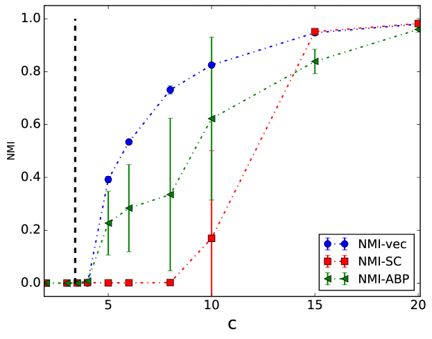
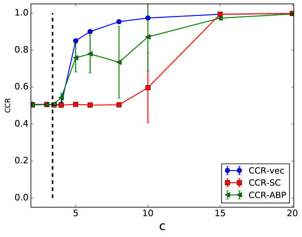
Figure 1: NMI ( top sub-figure, dashed curves) and CCR ( bottom sub-figure, solid curves) versus sparsity level $c$ for VEC, SC, and ABP on SBM graphs with constant degree scaling. Here, $\mathbf{p}$ is uniform, $K=2,\lambda=0.9$, and $n=10000$. The vertical dashed line is $c_{\text{weak}}=2.8$. This figure is best viewed in color.

To understand behavior around the weak recovery limit, we synthesized SBM graphs with $K=2$, $n=10000$, and $\lambda=0.9$ at various sparsity levels $c$ in the constant scaling regime. For these parameter settings, weak recovery is possible if, and only if, $c>c_{\text{weak}}\approx 2.8$ (cf. Condition 1). The results are summarized in Fig. 1.

Figure 1 reveals that the proposed VEC algorithm exhibits weak recovery phase transition behavior: for $c>c_{\text{weak}}$, $\text{CCR}>0.5$ and when $c<c_{\text{weak}}$, $\text{CCR}\approx 0.5$ (random guess). This behavior can be also observed through the NMI metric. The behavior of ABP which provably achieves the weak recovery limit [15] is also shown in Fig. 1. Compared to ABP, VEC has consistently superior mean clustering accuracy over the entire range of $c$ values. In addition, we note that the variance of NMI and CCR for ABP is significantly larger than VEC. This is discussed later in this section. SC, however, does not achieve weak recovery for sparse $c$ (cf. Fig. 1) which is consistent with theory [22].

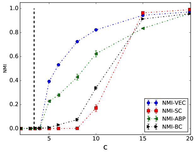
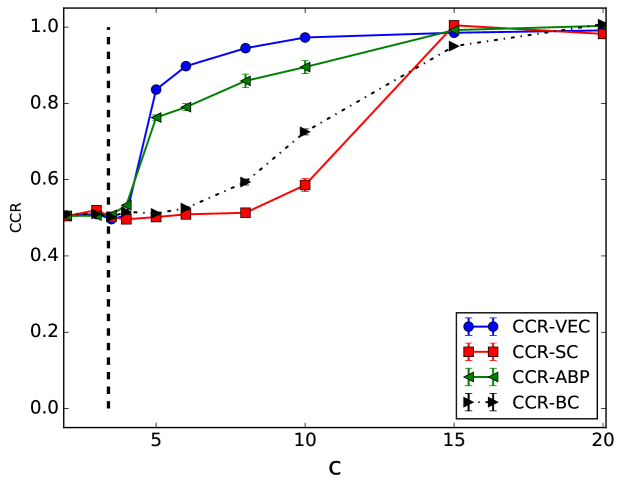
Figure 2: NMI ( top sub-figure, dashed curves) and CCR ( bottom sub-figure, solid curves) versus sparsity level $c$ for VEC, SC, and ABP on SBM graphs with constant degree scaling. Here, $\mathbf{p}$ is uniform, $K=2,\lambda=0.9$, and $n=10000$. The vertical dashed line is $c_{\text{weak}}=2.8$. Each CCR/NMI value is based on $500$ independent random graph realizations. Each point represents the mean CCR/NMI value and the associated confidence bar ($({\text{empirical std\_dev}})/\sqrt{500}$) are shown. The performance of BigClam (BC, [38]) is also shown. This figure is best viewed in color.

Effect of increasing number of random experiments: The curves shown in Fig. 1 are based on averaging performance metrics across multiple, independently generated, random realizations of SBM graphs. In order to understand the impact of the number of realizations on the overall performance trends of different algorithms, we increased the number of random graphs used to create each data point in Fig. 1 from $5$ to $500$. The resulting mean NMI and CCR values and their associated confidence intervals are shown in Fig. 2. Comparing the curves in Fig. 1 and Fig. 2, we see that they are very similar. The confidence intervals of all algorithms have clearly diminished as expected. Thery were already very small for VEC even with $5$ realizations. They have all but “disappeared” for VEC with $500$ realizations. The only significant change is to the mean curve for ABP which has become monotonic (as it should) and smoother after increasing the number of random realizations. Since the curves with $5$ and $500$ realizations are so similar, we only use $5$ random realizations for each SBM parameter setting in the rest of this paper.

Comparison with BigClam [38]: Figure 2 also shows the performance of BigClam [38] (BC) a recent powerful community detection algorithm based on matrix factorization techniques that scales well to large graphs of millions of nodes and edges. We observe that BC outperforms SC when the graph is relatively sparse. But VEC and ABP still outperform BC. Since the performance of BigClam is quite similar to that of SC, we decided to exclude BC in the remainder of our experiments.

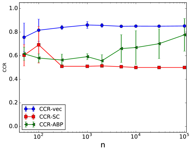
Figure 3: NMI ( top sub-figure, dashed curves) and CCR ( bottom sub-figure, solid curves) versus $n$ for VEC, SC, and ABP on SBM graphs with constant degree scaling. Here, $\mathbf{p}$ is uniform, $K=2,\lambda=0.9$, and $c=5.0>c_{\text{week}}$.

Effect of graph size: In order to provide further support for the observations presented above we also synthesized SBM graphs with increasing graph size $n$ with $K=2,\lambda=0.9,c=5.0$ held fixed in the constant degree scaling regime. Since $c=5.0>c_{\text{weak}}$, weak recovery is possible asymptotically as $n\rightarrow\infty$. As shown in Fig. 3, VEC can empirically achieve weak recovery for both small and large graphs, and consistently outperforms ABP and SC. While ABP can provably achieve weak recovery asymptotically, its performance on smaller graphs is poor.

Crossing below the weak recovery limit for $K>4$:

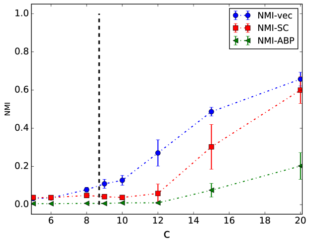
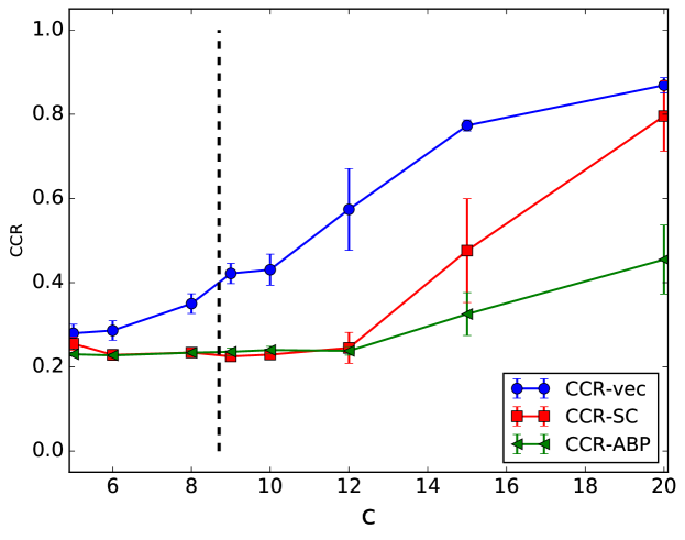
Figure 4: NMI ( top sub-figure, dashed curves) and CCR ( bottom sub-figure, solid curves) versus sparsity level $c$ for VEC, SC, and ABP on SBM graphs with constant degree scaling. Here, $\mathbf{p}$ is uniform, $K=5,\lambda=0.9$, and $n=1000$. The vertical dashed line is $c_{\text{weak}}=8.6$.

Here we explore the behavior of VEC below the weak recovery limit for $K>4$ since to-date there are no necessary and sufficient weak recovery bounds established for this setting (i.e., $K>4$). Similar to Fig. 1, we synthesized SBM graphs in the constant degree scaling regime for various sparsity levels $c$ fixing $K=5,\lambda=0.9$, and $n=1000$. In this setting, $c>c_{\text{weak}}=8.7$ is sufficient but not necessary for weak recovery. The results are summarized in Fig. 4.

As can be seen in Fig. 4, the VEC algorithm can cross the weak recovery limit: for some $c\leq c_{\text{weak}}$, $\text{CCR}>\frac{1}{K}$ and $\text{NMI}>0$ with a significant margin. Here too we observe that VEC consistently outperforms ABP and SC with a large margin.

Weak recovery with increasing number of communities $K$: Next we consider the performance of VEC as the number of communities $K$ increases. In particular, we synthesize planted partition model SBMs in the constant scaling regime with $c=10$, $\lambda=0.9$, $N=10000$, and uniform $\mathbf{p}$. As $K$ increases, recovery becomes impossible, because according to Condition 1 for weak recovery [15], weak recovery is possible if $\lambda^{2}c>K(1+(K-1)(1-\lambda))$. For the above parameter settings, we have $K\leq K_{\text{weak}}=5$.

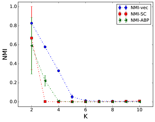
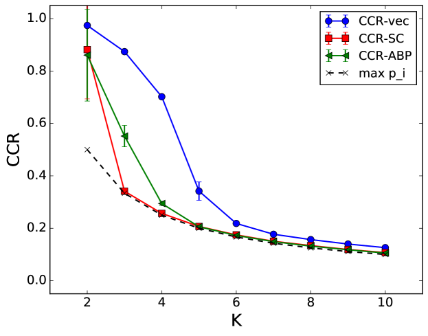
Figure 5: NMI ( top sub-figure, dashed curves) and CCR ( bottom sub-figure, solid curves) versus number of communities $K$ for VEC, SC, and ABP on SBM graphs with constant degree scaling. Here, $\mathbf{p}$ is uniform, $\lambda=0.9$, $c=10$, and $n=10000$. Weak recovery is possible if $K\leq K_{\text{weak}}=5$. The black dashed curve in the CCR sub-figure is the plot of the maximum community weight $\max_{k}p_{k}$ versus $K$. It is the CCR of the rule which assigns the apriori most likely community to all nodes.

Figure 5 summarizes the performance of VEC, SC, and ABP as a function of $K$. The performance of the three algorithms can be compared more straightforwardly by focusing on the NMI metric (plots in the upper sub-figure of Fig. 5). Similar to all the previous studies of this section, the proposed VEC algorithm can empirically achieve weak-recovery whenever the information-theoretic sufficient conditions are satisfied, i.e., $\text{NMI}>0$ with a significant margin for all $K\leq K_{\text{weak}}=5$. We note that in terms of the CCR metric, a “weak” recovery corresponds to $\text{CCR}>\max_{k}p_{k}\approx 1/K$ since $\max_{k}p_{k}$ it is the CCR of the rule which assigns the apriori most likely community label to all nodes. This is empirically attained by the VEC algorithm as illustrated in plots in the bottom sub-figure of Fig. 5.

Note that the performance of SC drops significantly beyond $K>2$. We also note that the CCR performance margin between ABP, which is a provably asymptotically consistent algorithm, and the best constant guess rule ($\text{CCR}=1/K$) is much smaller than for VEC.

IV-C Weak Recovery with Unbalanced Communities and Unequal Connectivities

Here we study how unbalanced communities and unequal connectivities affect the performance of the proposed VEC algorithm. By unbalanced communities we mean an SBM in which the community membership weights $\mathbf{p}$ are not uniform. In this scenario, some clusters will be more dominant than the others making it challenging to detect small clusters. By unequal connectivities we mean an SBM in which $\mathbf{Q}_{n}(k,k)$ is not the same for all $k$ or $\mathbf{Q}_{n}(k,k^{\prime})$ is not the same for all $k\neq k^{\prime}$. Since it is unwieldy to explore all types of unequal connectivities, our study only focuses on unequal self-connectivities, i.e., $\mathbf{Q}_{n}(k,k)$ is not the same for all $k$. In this scenario, the densities of different communities will be different making it challenging to detect the sparser communities. Here we compare NMI and CCR curves only for VEC and ABP but not SC. When communities are unbalanced or the self-connectivities are unequal we observed that SC takes an inordinate amount of time to terminate. We decided therefore to omit NMI and CCR plots for SC from the experimental results in this subsection.

Unbalanced communities: We first show results on SBMs with nonuniform community weights $\mathbf{p}$. For simplicity, we consider SBMs with $K=2$ communities and set $p_{1}=\gamma\in\left[0.5,1\right)$. Then, $p_{2}=1-\gamma$. For the other parameters we set $c=8,N=10000,\lambda=0.9$. From the general weak recovery conditions for nonuniform ${\bf p}$ in [15], it can be shown that as $\gamma\rightarrow 1$, the threshold for guaranteed weak-recovery will be broken. Specifically, for the above parameter settings, it can can be shown that $\gamma$ must not exceed $\gamma_{\text{weak}}\approx 0.65$ for weak recovery.

We summarize the results in Fig. 6. For comparison, the right (CCR) sub-figure of Fig. 6 also shows the plot of $\max_{k}p_{k}=\gamma$ which is the CCR of the rule which assigns the apriori most likely community to all nodes. From the figure it is evident that unlike ABP, the CCR performance of VEC remains stable across a wide range of $\gamma$ values indicating that it can tolerate significantly unbalanced communities.

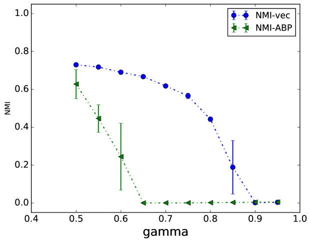
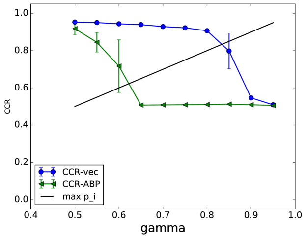
Figure 6: NMI ( top sub-figure, dashed curves) and CCR ( bottom sub-figure, solid curves) versus maximum community weight $\gamma$ for VEC and ABP on SBM graphs with constant degree scaling. Here, $K=2$, $\mathbf{p}=\left[\gamma,1-\gamma\right]$, $\lambda=0.9$, $c=8$, and $n=10000$. Weak recovery is possible if $\gamma\leq\gamma_{\text{weak}}=0.65$. The solid unmarked curve in the CCR sub-figure indicates the maximum community weights $\max_{k}p_{k}=\gamma$ in each setting. It is the CCR of the rule which assigns the apriori most likely community to all nodes.

Unequal community connectivity: We next consider the situation in which the connectivity constants of different communities are distinct. For simplicity, we consider SBMs with $K=2$ communities and balanced weights $p_{1}=p_{2}=0.5$. We focus on the constant scaling regime and set

$$Q_{n}=\begin{bmatrix}\frac{c}{n}&\frac{c(1-\lambda)}{n}\\ \frac{c(1-\lambda)}{n}&\frac{c\beta}{n}\end{bmatrix}$$

Here, $\beta\in\left(0,1\right]$ determines the relative densities of communities $1$ and $2$. For the other model parameters, we set $c=8$, $\lambda=0.9$ as in the previous subsection. From the general weak recovery conditions for unequal community connectivity in [15], it can be shown that weak recovery requires that $\beta\geq\beta_{\text{weak}}\approx 0.60$. We summarize the results in Fig. 7.

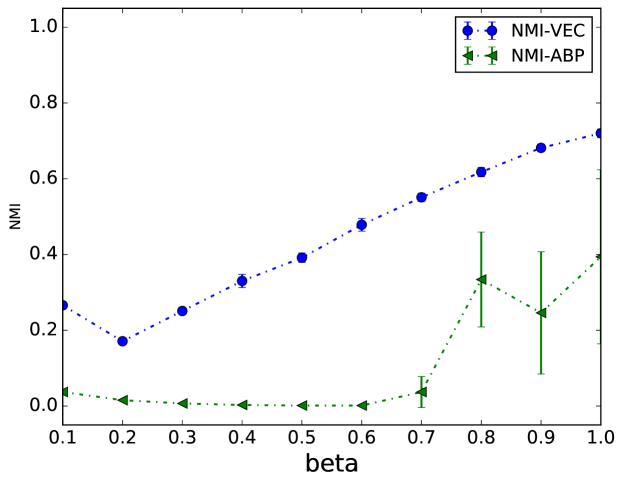
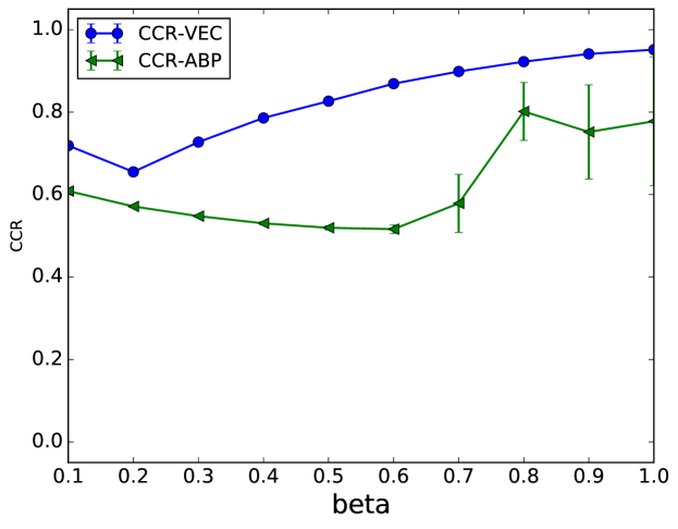
Figure 7: NMI ( top sub-figure, dashed curves) and CCR ( bottom sub-figure, solid curves) versus community connectivity $\beta$ for VEC and ABP on SBM graphs with constant degree scaling. Here, $\mathbf{p}$ is uniform, $\lambda=0.9$, $c=8$ and $n=10000$. Weak recovery is possible if $\beta\leq\beta_{\text{weak}}=0.60$. The dashed curve in the CCR sub-figure is the maximum community weight $\max_{k}p_{k}$ in each setting. It is the CCR of the rule which assigns the apriori most likely community to all nodes.

From the figure it is once again evident that the performance of VEC remains stable across a wide range of $\beta$ values when compared to ABP.

IV-D Exact Recovery Limits

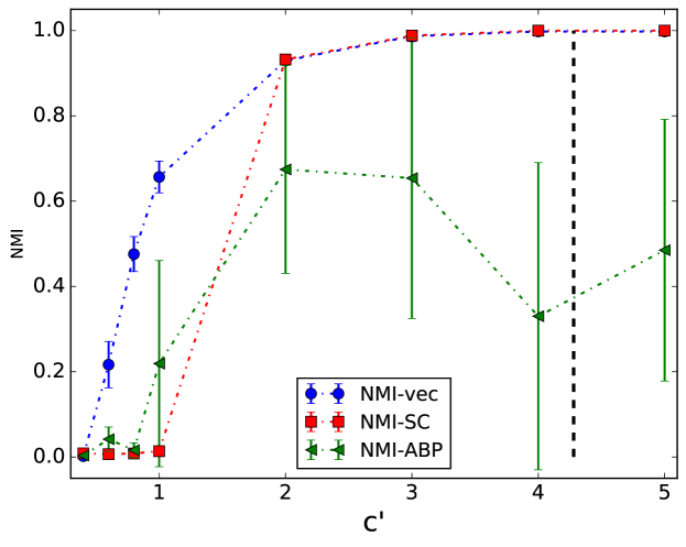
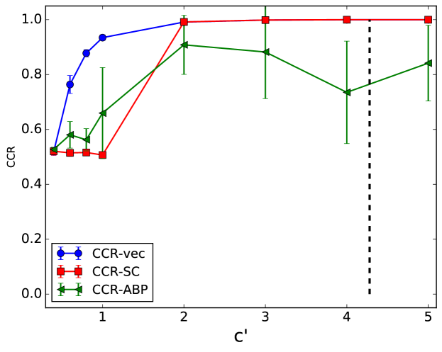
Figure 8: NMI ( top sub-figure, dashed curves) and CCR ( bottom sub-figure, solid curves) versus sparsity level $c^{\prime}$ for VEC, SC, and ABP on SBM graphs with logarithmic scaling. Here, $\mathbf{p}$ is uniform, $K=2,\lambda=0.9$, and $n=10000$. The vertical dashed-line is at $c^{\prime}_{\text{exact}}=4.3$.

We now turn to explore the behavior of VEC near the exact recovery limit. Figure 8 plots NMI and CCR as a function of increasing sparsity level $c^{\prime}$ for SBM graphs under logarithmic node degree scaling fixing $K=2$, $N=10000$, and $\lambda=0.9$. In this setting, exact recovery is solvable if, and only if, $c^{\prime}>c^{\prime}_{\text{exact}}\approx 4.3$ (cf. Condition 2 in Sec. IV-A). As can be seen in Fig. 8, the CCR and NMI values of VEC converge to $1.0$ as $c^{\prime}$ increases far beyond $c^{\prime}_{\text{exact}}$. Therefore, VEC empirically attains the exact recovery limit. We note that SC can match the performance of VEC when $c^{\prime}$ is large, but cannot correctly detect communities for very sparse graphs ($c^{\prime}\leq 1$). Note also that VEC significantly outperforms ABP in this scaling scheme.

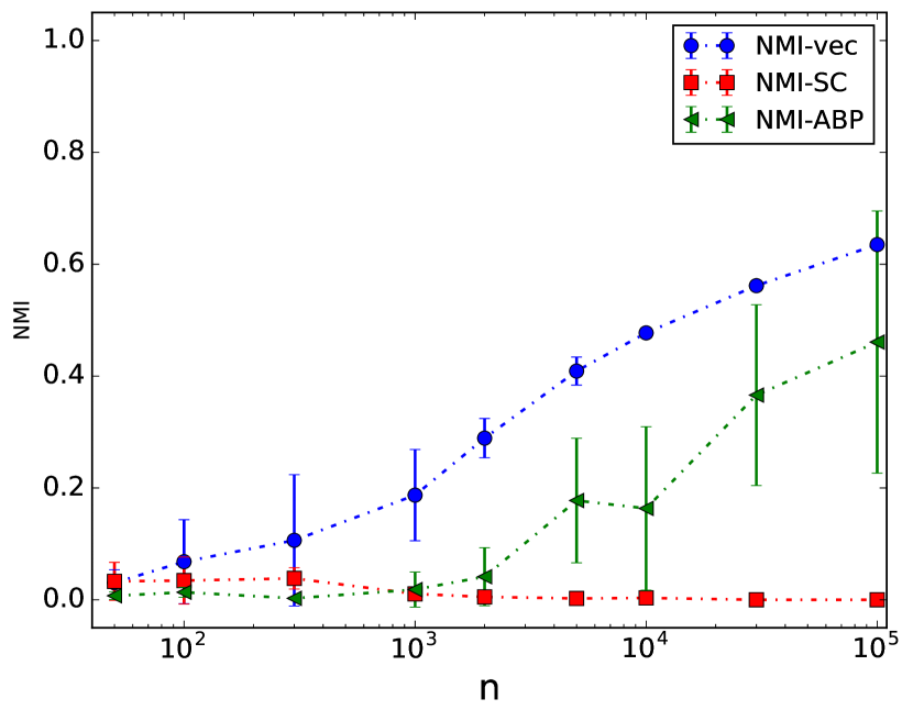
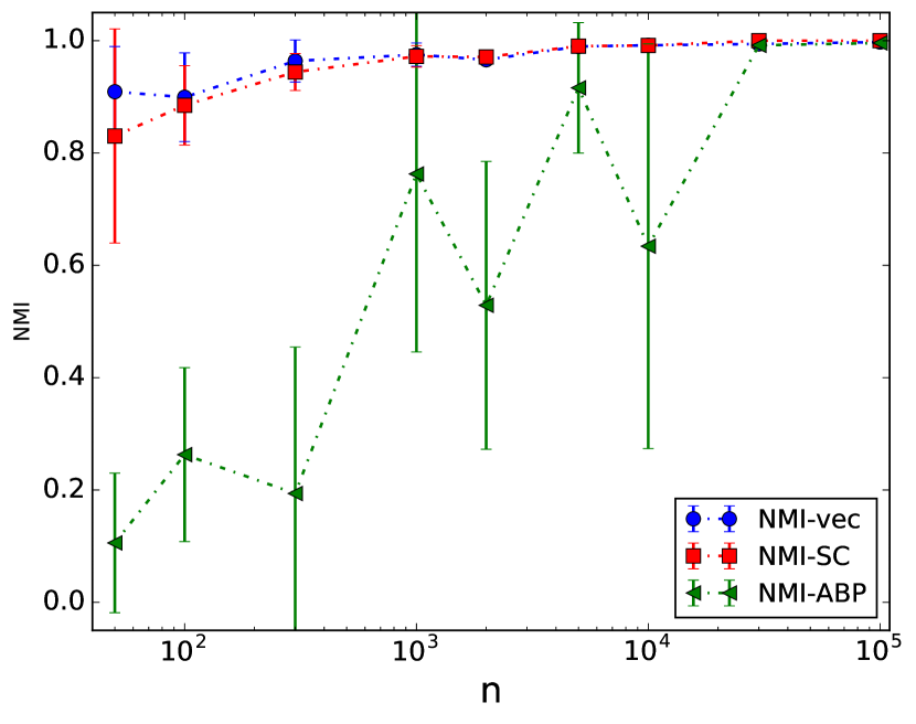
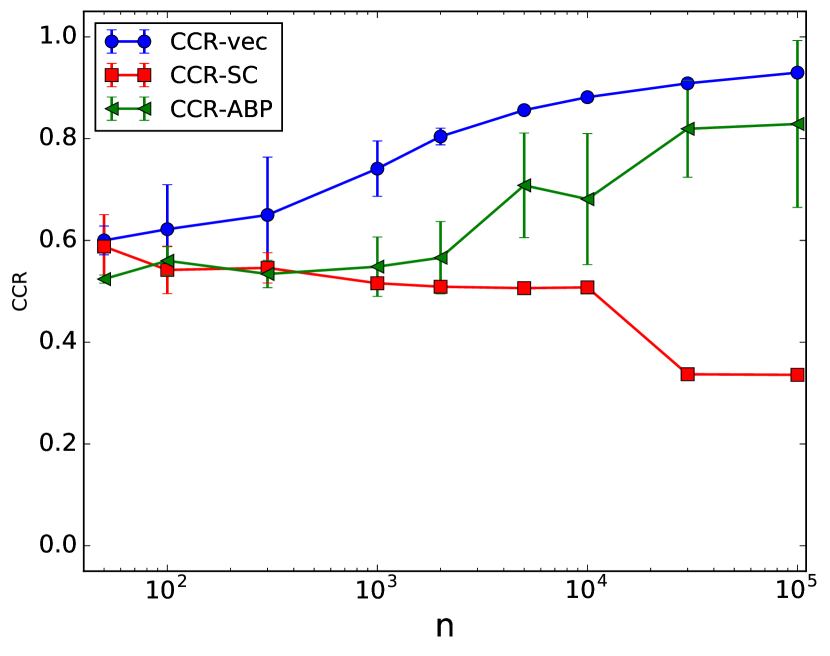
(a) $c^{\prime}=0.6$

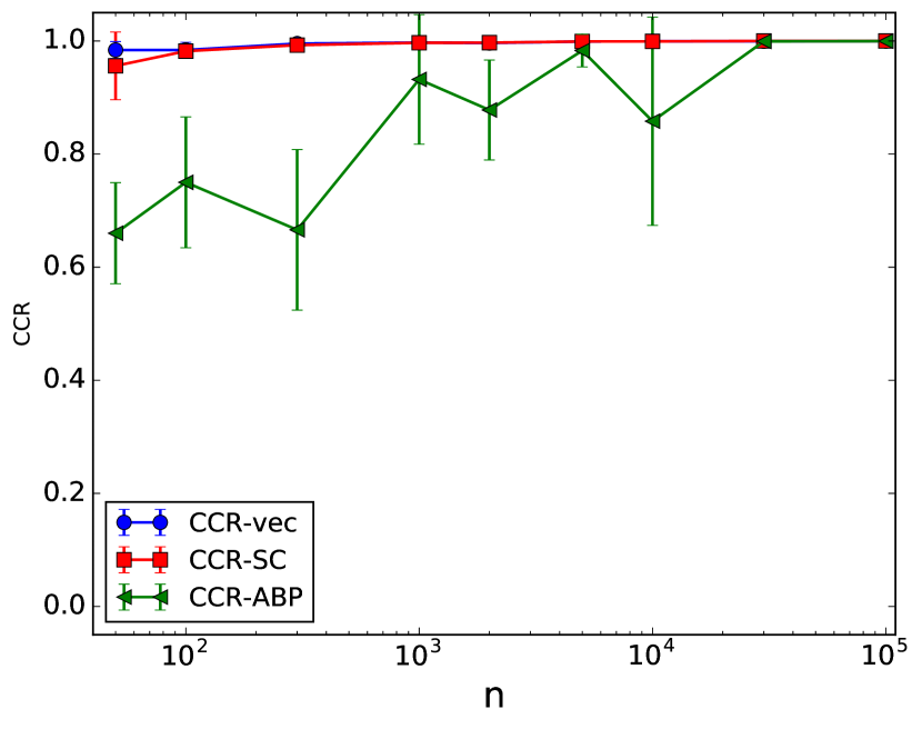
(b) $c^{\prime}=2.5$

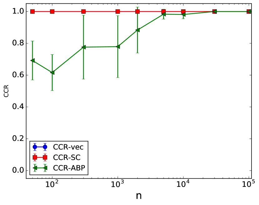
(c) $c^{\prime}=4.5$

Figure 9: NMI (top sub-figure, dashed curves) and CCR (bottom sub-figure, solid curves) versus number of nodes $n$ for VEC, SC, and ABP on SBM graphs with logarithmic scaling. Here, $\mathbf{p}$ is uniform, $K=2$, and $\lambda=0.9$. In subplots $(a)$ and $(b)$, $c^{\prime}<c_{\text{exact}}^{\prime}$ while in subplot $(c)$, $c^{\prime}>c_{\text{exact}}^{\prime}$. We note that in subplot $(c)$, the curves of VEC and SC are on top of each other since they have very similar performance in this setting.

We also compared the behavior of VEC, ABP, and SC algorithms for increasing graph sizes $n$. We set $K=2,\lambda=0.9$, and $\mathbf{p}\sim$ uniform. Figure 9 illustrates the performance of VEC, SC, and ABP as a function of the number of nodes $n$ for three different choices of $c^{\prime}:c^{\prime}=0.6,2.5$, and $4.5$. Since exact recovery requires $c^{\prime}\geq c^{\prime}_{\text{exact}}\approx 4.3$, only the third choice of $c^{\prime}$ guarantees exact recovery asymptotically.

As can be seen in Fig. 9, when $c^{\prime}$ is above the exact recovery condition (see Fig. 9 $(c)$), the proposed algorithm VEC can achieve exact recovery, i.e., $\text{CCR}\approx 1$ and $\text{NMI}\approx 1$. In this setting, the proposed VEC algorithm can be observed to achieve exact recovery even when the number of nodes $n$ is relatively small. On the other hand, when $c^{\prime}$ is below the exact recovery condition (see Figs. 9 $(a)$ and $(b)$), as $n$ increases, the accuracy of VEC increases and converges to a value that is somewhere between random guessing ($\text{CCR}=0.5,\text{NMI}=0.0$) and exact recovery ($\text{CCR}=1.0,\text{NMI}=1.0$).

We note that among the compared baselines, the performance of SC is similar to that of VEC when $c^{\prime}$ is large (relatively dense graph) but its performance deteriorates when $c^{\prime}$ is small (sparse graph). As shown in Fig. 9 $(a)$, when the SBM-synthesized graph is relatively sparse, the performance of SC is close to a random guess while the performance of VEC and ABP increases with the number of nodes $n$. This observation is consistent with known theoretical results [11, 23].

IV-E Robustness of proposed approach

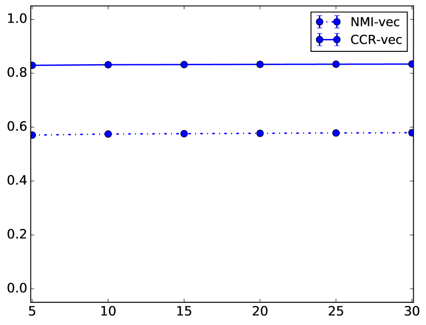
(a) $r$

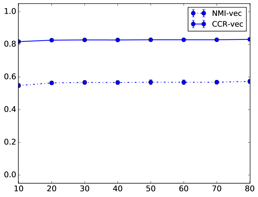
(b) $\ell$

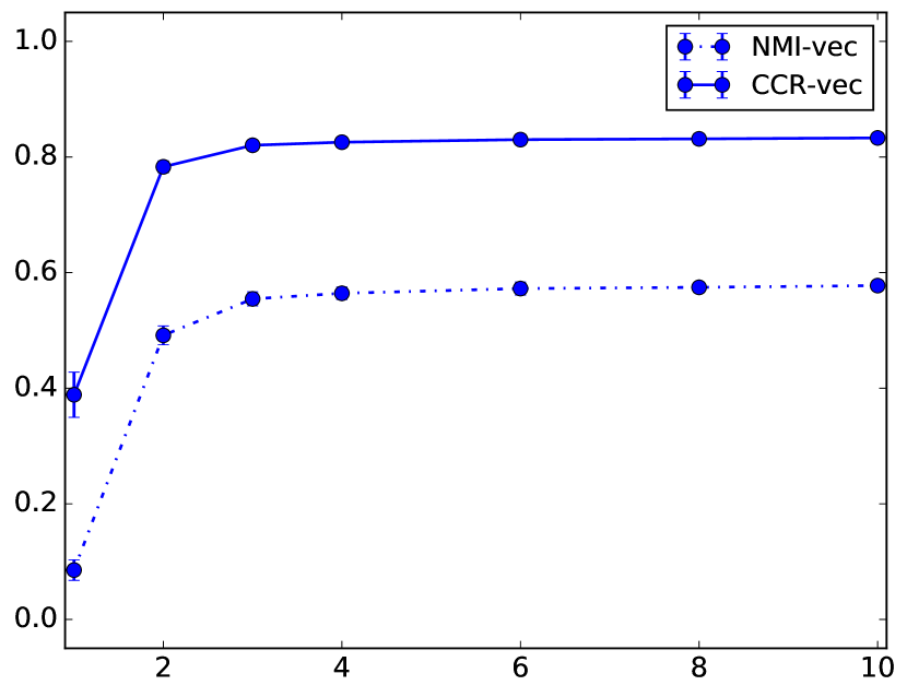
(c) $w$

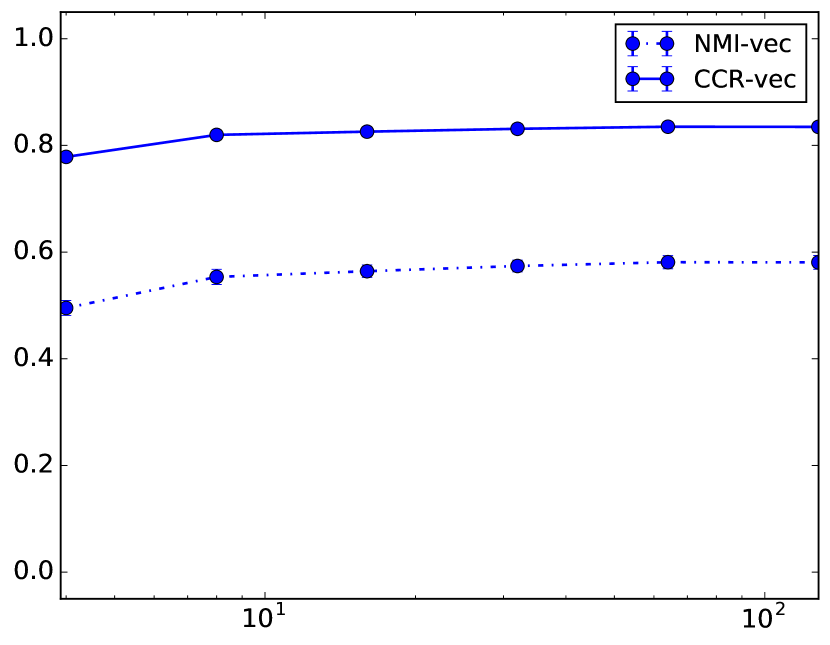
(d) $\log(d)$

Figure 10: NMI (dashed curves) and CCR (solid curves) as a function of different algorithm parameters of VEC on SBM graphs: (a) the number of random paths simulated from each node $r$, (b) the length of each random path $\ell$, (c) the size of the local window $w$, and (d) the embedding dimension $d$. In each subplot, only one parameter is varied keeping others fixed. When fixed, the default parameter values are $r=10,\ell=60,w=8,d=50$.

Parameter sensitivity: The performance of VEC depends on the number of random paths per node $r$, the length of each path $\ell$, the local window size $w$, and the embedding dimension $d$. We synthesized SBM graphs under logarithmic scaling with $K=5,N=10,000,c^{\prime}=2,\lambda=0.9$ and applied VEC with different choices for $r$, $\ell$, $w$, and $d$. The results are summarized in Fig. 10. While the performance of VEC is remarkably insensitive to $r$, $\ell$, and $d$ across a wide range of values, a relatively large local window size $w\geq 3$ appears to be essential for attaining good performance (cf. Fig. 10(c)). This suggests that incorporating a larger graph neighborhood is critical to the success of VEC.

Effect of random initialization in VEC and ABP: We also studied the effect of random initialization in VEC and ABP. We synthesized two SBM graphs as described in Table II. For a fixed graph, we run VEC and ABP $10$ times and summarize the mean and standard deviation values of NMI and CCR. We observe that the variance of ABP is an order of magnitude higher than VEC indicating its high sensitivity to initialization.

TABLE II: Means and standard deviations of NMI and CCR for $10$ runs on the same graph. Sim1: a graph with constant scaling, $K=5,N=10000,c=15.0,\lambda=0.9$. Sim2: a graph with logarithmic scaling, $K=2,N=10000,c^{\prime}=2.0,\lambda=0.9$.

	NMI		CCR
Expt.	VEC	ABP	VEC	ABP
Sim1	$0.42\pm 0.004$	$0.14\pm 0.03$	$0.74\pm 0.002$	$0.42\pm 0.06$
Sim2	$0.96\pm 0.002$	$0.73\pm 0.37$	$0.99\pm 0.0003$	$0.93\pm 0.15$

IV-F Summarizing overall performance via Performance Profiles

So far we presented and discussed the performance of VEC, ABP, and SC across a wide range of parameter settings. All results indicate that VEC matches or outperforms both ABP and SC in almost all scenarios. In order to summarize and compare of the overall performance of all three algorithms across the wide range of parameter settings that we have considered, we adopt the commonly used Performance Profile [40] as a “global” evaluation metric. Formally, let $\mathcal{P}$ denote a set of experiments and $a$ a specific algorithm. Let $Q(a,e)$ denote the value of a performance metric attained by an algorithm $a$ in experiment $e$ where higher $Q$ values correspond to better performance. Then the performance profile of $a$ at $\tau\in[0,1]$ is the fraction of the experiments in which the performance of $a$ is at least a factor $(1-\tau)$ times as good as the best performing algorithm in that experiment, i.e.,

$$PP_{a}(\tau):=\frac{|\{e:Q(a,e)\geq(1-\tau)\max_{a^{\prime}}Q(a^{\prime},e)\}|}{|\mathcal{P}|}$$ (4)

The Performance Profile is thus an empirical cumulative distribution function of an algorithm’s performance relative to the best-performing algorithm in each experiment. We calculate $PP_{a}(\tau)$ for $\tau\in(0,1)$. The higher a curve corresponding to an algorithm, the more often it outperforms the other algorithms.

For simplicity, we only consider the simulation settings for the planted partition model SBMs in the constant degree scaling regime. We set $c\in\{2,5,10,15\}$, $K\in\{2,5,10\}$, and $N\in\{1e2,1e3,1e4,1e5\}$. For each combination of settings $(c,K,N)$, we conduct $5$ independent random repetitions of the experiment. Thus overall the Performance Profile is calculated based on $240$ experiments.

Figure 11 shows the performance profiles for both NMI and CCR metrics. From the figure it is clear that VEC dominates both ABP and SC and that ABP and SC have similar performance across many experiments.

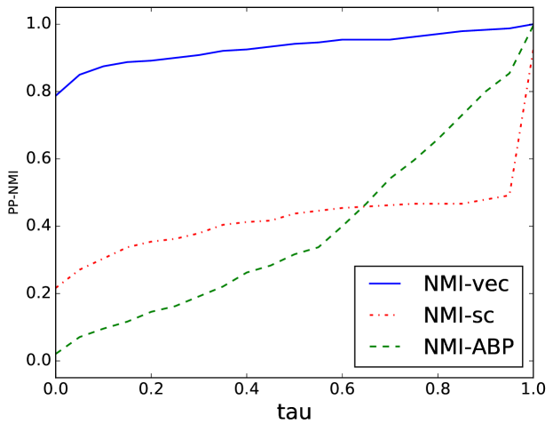
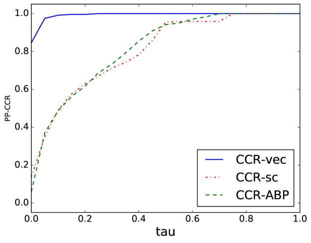
Figure 11: NMI (top sub-figure) and CCR (bottom sub-figure) Performance Profiles for VEC, SC, and ABP on SBM graphs with constant degree scaling. Here, $c\in\{2,5,10,15\}$, $K\in\{2,5,10\}$, $N\in\{1e2,1e3,1e4,1e5\}$, and $5$ random runs for each combination of settings for a total of $240$ distinct experiments.

IV-G Degree-corrected SBM

Our experiments thus far focused on the SBM where the expected degree is constant across all nodes within the same community (degree homogeneity). In order to compare the robustness of different algorithms to degree heterogeneity, we considered the degree-corrected SBM [41] (DC-SBM), which generates edge-weighted graphs with a power law within-community degree distribution that is observed in many real-world graphs. We adopted the following generative procedure which was proposed in [41]: (1) Assign the latent community labels using the same procedure as in the SBM; (2) Within each community, sample a parameter $\theta_{i}$ from a power law distribution for each node $i$ within this community, and normalize these $\theta_{i}$’s so that they sum up to $1$; (3) For any two nodes $i$ and $j$, sample a weighted edge $\{i,j\}$ with weights drawn from a Poisson distribution with mean $\theta_{i}\theta_{j}Q_{n}(\pi_{i},\pi_{j})$. We omitted the steps of generating self-loops since they will be ignored by the community detection algorithms. Our proposed algorithm VEC can be modified to handle weighted graphs by setting the random walk transition probabilities to be proportional to the edge weights. The ABP and SC algorithms can also be suitably adapted to work with weighted graphs.

We simulated graphs with $n=1000,\lambda=0.9$ and the power law distribution for $\theta_{i}$ with power $-2.5$ and a minimum $\theta_{i}$ value of $10$. We considered a number of sparsity settings used to simulate SBM graphs in previous sections. For each setting, the mean NMI and CCR values and their confidence intervals (based on $500$ random graphs ) are summarized in Table III. These results indicate that our algorithm still outperforms the competing approaches. We would like to point out that even though the DC-SBM and SBM parameters are similar, the similarity of parameter settings does not imply similarity of information-theoretic limits. To the best of our knowledge, the information-theoretic limits of recovery for the DC-SBM is still open.

TABLE III: Results for degree-corrected SBM graphs.

Setting	NMI			CCR
	VEC	SC	ABP	VEC	SC	ABP
$K=2,c=10$, constant scaling	$0.610\pm 0.057$	$0.007\pm 0.01$	$0.008\pm 0.05$	$0.920\pm 0.02$	$0.512\pm 0.01$	$0.519\pm 0.04$
$K=5,c=10$, constant scaling	$0.167\pm 0.02$	$0.022\pm 0.01$	$0.006\pm 0.01$	$0.418\pm 0.03$	$0.224\pm 0.001$	$0.227\pm 0.02$
$K=2,c^{\prime}=2$, log scaling	$0.737\pm 0.07$	$0.018\pm 0.04$	$0.014\pm 0.07$	$0.953\pm 0.02$	$0.515\pm 0.02$	$0.522\pm 0.04$
$K=5,c^{\prime}=2$, log scaling	$0.295\pm 0.05$	$0.018\pm 0.01$	$0.007\pm 0.01$	$0.573\pm 0.07$	$0.224\pm 0.01$	$0.226\pm 0.02$

V Experiments with Real-World Graphs

Having comprehensively studied the empirical performance of VEC, ABP, and SC on SBM-based synthetic graphs, in this section we turn our attention to real-world datasets that have ground truth (non-overlapping) community labels. Here we use only NMI[9] to measure the performance.

We consider two benchmark real-world graphs: the Political Blogs network [42] and the Amazon co-purchasing network [43]. Since the original graphs are directed, we convert it to undirected graphs by forming an edge between two nodes if either direction is part of the original graph. The basic statistics of the datasets are summarized in Table IV. Here, $\hat{\lambda}$ and $\hat{c^{\prime}}$ are the maximum likelihood estimates of $\lambda$ and $c^{\prime}$ respectively in the planted partition model SBM under logarithmic scaling. Note that in Amazon, the ground truth community proportions are highly unbalanced.

TABLE IV: Summary of real-world dataset parameters.

Dataset	$n$	$K$	# edges	$\hat{\lambda}$	$\hat{c^{\prime}}$	$\max_{k}\hat{p}_{k}$
Blogs	$1,222$	$2$	$16,714$	$0.89$	$6.9$	$0.52$
Amazon	$334,844$	$4$	$925,803$	$0.94$	$0.7$	$0.74$

We report NMI and CCR values for VEC, SC, and ABP applied to these datasets. To apply ABP, we set the algorithm parameters using the fitted SBM parameters as suggested in [15]. As shown in Table V, VEC achieves better accuracy compared to SC and ABP.

TABLE V: Results on real-world datasets.

	NMI			CCR
Data	VEC	SC	ABP	VEC	SC	ABP
Blogs	$0.745$	$0.002$	$0.686$	$0.954$	$0.529$	$0.925$
Amazon	$0.310$	$0.006$	$0.025$	$0.783$	$0.742$	$0.762$

The performance of SC is noticeably poorer (in terms of both NMI and CCR) compared to both VEC and ABP. Interestingly, the NMI of SC on random graphs that are synthetically generated according to a planted partition SBM model that best fits (in a maximum-likelihood sense) the Political Blogs graph is surprisingly good: NMI = $1.0$ (average NMI across 10 random graphs). This suggests that real-world graphs such as Political Blogs have additional characteristics that are not well-captured by a planted partition SBM model. This is further confirmed by the plots of empirical degree distributions of nodes in real-world and synthesized graphs in Fig. 12. The plots show that the node degree distributions are quite different in real-world and synthesized graphs even if the SBM model which is used to generate the graphs is fitted in a maximum-likelihood sense to real-world graphs. These results also suggest that the performance of SC is sensitive to model-mismatch and its good performance on synthetically generated graphs based on SBMs may not be indicative of good performance on matching real-world graphs. In contrast to SC, both VEC and ABP do not seem to suffer from this limitation.

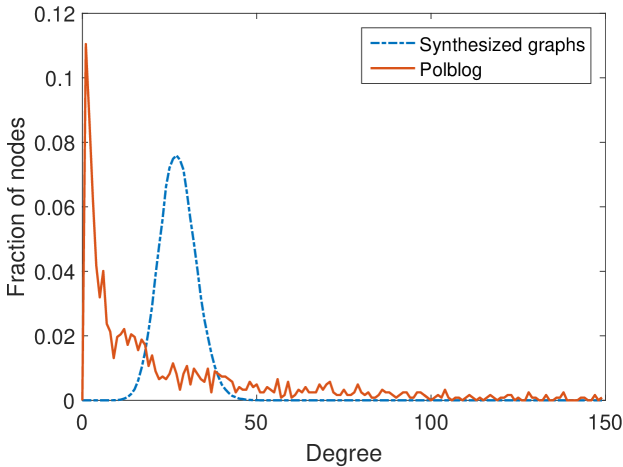
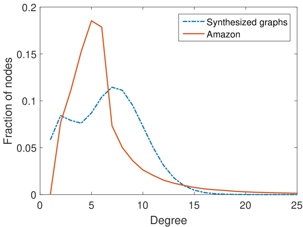
Figure 12: Empirical degree distributions of real and synthesized graphs (averaged over 200 trials) for the Political Blogs (top) and Amazon (bottom) datasets. The error bars are too small to be visible in the plots and have been omitted. The distributions have long tails and are truncated in the figure for better of visualization.

Finally, we also visualize the learned embeddings in Political Blogs using the now-popular t-Distributed Stochastic Neighbor Embedding (t-SNE) tool [44] in Fig. 13. The picture is consistent with the intuition that nodes from the same community are close to each other in the latent embedding space.

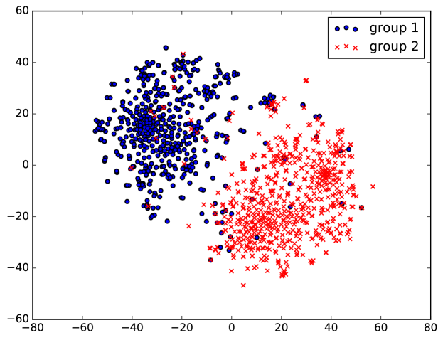
Figure 13: t-SNE visualization of learned embedding vectors in the Blogs dataset. The markers reflect ground-truth groups.

VI Concluding Remarks

In this work we put forth a novel framework for community discovery in graphs based on node embeddings. We did this by first constructing, via random walks in the graph, a document made up of sentences of node-paths and then applying a well-known neural word embedding algorithm to it. We then conducted a comprehensive empirical study of community recovery performance on both simulated and real-world graph datasets and demonstrated the effectiveness and robustness of the proposed approach over two state-of-the-art alternatives. In particular, the new method is able to attain the information-theoretic limits for recovery in stochastic block models.

There are a number of aspects of the community recovery problem that we have not explored in this work, but which merit further investigation. First, we have focused on undirected graphs, but our algorithm can be applied ‘as-is’ to directed graphs as well. We have assumed knowledge of the number of communities $K$, but the node embedding part of the algorithm itself does not make use of this information. In principle, we can apply any $K$-agnostic clustering algorithm to the node embeddings. We have focused on non-overlapping community detection. It is certainly possible to convert an overlapping community detection problem with $K$ communities into a non-overlapping community detection problem with $2^{K}$ communities, but this approach is unlikely to work well in practice if $K$ is large. An alternative approach is to combine the node embeddings with topic models to produce a “soft” clustering. Finally, this study was purely empirical in nature. Establishing theoretical performance guarantees that can explain the excellent performance of our algorithm is an important task which seems challenging at this time. One difficulty is the nonconvex objective function of the word2vec algorithm. This can be partially addressed by constructing a suitable convex relaxation and analyzing its limiting behavior (under suitable scaling) as the length of the random walk goes to infinity. The limiting objective function will still be random since it depends on the observed realization of the random graph. One could then examine if the limiting objective, when suitably normalized, concentrates around its mean value as the graph size goes to infinity.

References

- [1] Y. Bengio, A. Courville, and P. Vincent, “Representation learning: A review and new perspectives,” IEEE transactions on pattern analysis and machine intelligence, vol. 35, no. 8, pp. 1798–1828, 2013.
- [2] M. Belkin and P. Niyogi, “Laplacian eigenmaps and spectral techniques for embedding and clustering,” in Advances in Neural Information Processing Systems, 2002, pp. 585–591.
- [3] B. Perozzi, R. Al-Rfou, and S. Skiena, “Deepwalk: Online learning of social representations,” in Proc. of the 20th ACM SIGKDD International Conference on Knowledge Discovery and Data Mining (KDD), Aug. 2014, pp. 701–710.
- [4] Z. Yang, W. Cohen, and R. Salakhutdinov, “Revisiting semi-supervised learning with graph embeddings,” arXiv preprint arXiv:1603.08861, 2016.
- [5] F. McSherry, “Spectral partitioning of random graphs,” in Foundations of Computer Science (FOCS), 2001 IEEE 42th Annual Symposium on, 2001, pp. 529–537.
- [6] W. Chen, Y. Song, H. Bai, C. Lin, and E. Chang, “Parallel spectral clustering in distributed systems,” IEEE Transactions on Pattern Analysis and Machine Intelligence, vol. 33, no. 3, pp. 568–586, 2011.
- [7] T. Mikolov, I. Sutskever, K. Chen, G. S. Corrado, and J. Dean, “Distributed representations of words and phrases and their compositionality,” in Advances in neural information processing systems, 2013, pp. 3111–3119.
- [8] A. Grover and J. Leskovec, “node2vec: Scalable feature learning for networks,” in Proc. of the 20th ACM SIGKDD International Conference on Knowledge Discovery and Data Mining (KDD), Aug. 2016.
- [9] A. Lancichinetti and S. Fortunato, “Community detection algorithms: A comparative analysis,” Physical Review E, vol. 80, p. 056117, Nov 2009.
- [10] S. Fortunato, “Community detection in graphs,” Physics reports, vol. 486, no. 3, pp. 75–174, 2010.
- [11] E. Abbe and C. Sandon, “Community detection in general stochastic block models: Fundamental limits and efficient algorithms for recovery,” in Proc. of the 56th Annual Symposium on Foundations of Computer Science (FOCS), Sep. 2015, pp. 670–688.
- [12] J. Yang and J. Leskovec, “Defining and evaluating network communities based on ground-truth,” Knowledge and Information Systems, vol. 42, no. 1, pp. 181–213, 2015.
- [13] E. Mossel, J. Neeman, and A. Sly, “Belief propagation, robust reconstruction and optimal recovery of block models,” in Proc. of the 27th Conference on Learning Theory (COLT), 2014, pp. 356–370.
- [14] A. Decelle, F. Krzakala, C. Moore, and L. Zdeborová, “Asymptotic analysis of the stochastic block model for modular networks and its algorithmic applications,” Physical Review E, vol. 84, no. 6, p. 066106, 2011.
- [15] E. Abbe and C. Sandon, “Detection in the stochastic block model with multiple clusters: proof of the achievability conjectures, acyclic bp, and the information-computation gap,” in Advances in Neural Information Processing Systems (NIPS), Dec. 2016.
- [16] H. White, S. Boorman, and R. Breiger, “Social structure from multiple networks, blockmodels of roles and positions,” American Journal of Sociology, pp. 730–780, 1976.
- [17] M. Newman, D. Watts, and S. Strogatz, “Random graph models of social networks,” Proc. of the National Academy of Sciences, vol. 99, no. 1, pp. 2566–2572, 2002.
- [18] J. Leskovec, K. Lang, A. Dasgupta, and M. Mahoney, “Statistical properties of community structure in large social and information networks,” in Proc. of the 17th International Conference on World Wide Web (WWW). ACM, 2008, pp. 695–704.
- [19] D. I. Shuman, S. K. Narang, P. Frossard, A. Ortega, and P. Vandergheynst, “The emerging field of signal processing on graphs: Extending high-dimensional data analysis to networks and other irregular domains,” IEEE Signal Processing Magazine, vol. 30, no. 3, pp. 83–98, 2013.
- [20] P. Holland, K. Laskey, and S. Leinhardt, “Stochastic blockmodels: First steps,” Social Networks, vol. 5, no. 2, pp. 109–137, 1983.
- [21] R. Boppana, “Eigenvalues and graph bisection: An average-case analysis,” in Proc. of the 28th Anuual Symposium on Foundations of Computer Science (FOCS), 1987, pp. 280–285.
- [22] J. Lei and A. Rinaldo, “Consistency of spectral clustering in stochastic block models,” The Annals of Statistics, vol. 43, no. 1, pp. 215–237, 2015.
- [23] K. Rohe, S. Chatterjee, and B. Yu, “Spectral clustering and the high-dimensional stochastic blockmodel,” The Annals of Statistics, vol. 39, no. 4, pp. 1878–1915, 2011.
- [24] B. Hajek, Y. Wu, and J. Xu, “Achieving exact cluster recovery threshold via semidefinite programming,” IEEE Transactions on Information Theory, vol. 62, no. 5, pp. 2788–2797, 2016.
- [25] P.-Y. Chen and A. O. Hero, “Phase transitions and a model order selection criterion for spectral graph clustering,” arXiv preprint arXiv:1604.03159, 2016.
- [26] M. Newman, “Community detection in networks: Modularity optimization and maximum likelihood are equivalent,” arXiv preprint arXiv:1606.02319, 2016.
- [27] J. Pennington, R. Socher, and C. D. Manning, “Glove: Global vectors for word representation.” in EMNLP, vol. 14, 2014, pp. 1532–43.
- [28] D. A. Spielman and S.-H. Teng, “Nearly-linear time algorithms for graph partitioning, graph sparsification, and solving linear systems,” in Proceedings of the thirty-sixth annual ACM symposium on Theory of computing. ACM, 2004, pp. 81–90.
- [29] R. Andersen, F. Chung, and K. Lang, “Local graph partitioning using pagerank vectors,” in Foundations of Computer Science, 2006. FOCS’06. 47th Annual IEEE Symposium on. IEEE, 2006, pp. 475–486.
- [30] R. Lambiotte, J.-C. Delvenne, and M. Barahona, “Random walks, markov processes and the multiscale modular organization of complex networks,” IEEE Transactions on Network Science and Engineering, vol. 1, no. 2, pp. 76–90, 2014.
- [31] R. Hamon, P. Borgnat, P. Flandrin, and C. Robardet, “From graphs to signals and back: Identification of network structures using spectral analysis,” arXiv preprint arXiv:1502.04697, 2015.
- [32] N. Tremblay and P. Borgnat, “Graph wavelets for multiscale community mining,” IEEE Transactions on Signal Processing, vol. 62, no. 20, pp. 5227–5239, 2014.
- [33] T. N. Kipf and M. Welling, “Semi-supervised classification with graph convolutional networks,” arXiv preprint arXiv:1609.02907, 2016.
- [34] O. Levy and Y. Goldberg, “Neural word embedding as implicit matrix factorization,” in Advances in neural information processing systems, 2014, pp. 2177–2185.
- [35] L. Bottou, “Large-scale machine learning with stochastic gradient descent,” in Proceedings of COMPSTAT’2010. Springer, 2010, pp. 177–186.
- [36] ——, “Online algorithms and stochastic approximations,” in Online Learning and Neural Networks, D. Saad, Ed. Cambridge, UK: Cambridge University Press, 1998, revised, oct 2012. [Online]. Available: http://leon.bottou.org/papers/bottou-98x
- [37] B. Recht, C. Re, S. Wright, and F. Niu, “Hogwild: A lock-free approach to parallelizing stochastic gradient descent,” in Advances in Neural Information Processing Systems, 2011, pp. 693–701.
- [38] J. Yang and J. Leskovec, “Overlapping community detection at scale: a nonnegative matrix factorization approach,” in Proceedings of the sixth ACM international conference on Web search and data mining. ACM, 2013, pp. 587–596.
- [39] K. P. Murphy, Machine learning: a probabilistic perspective. MIT press, 2012.
- [40] E. Dolan and J. Moré, “Benchmarking optimization software with performance profiles,” Mathematical Programming, vol. 91, no. 2, pp. 201–213, 2002.
- [41] B. Karrer and M. E. Newman, “Stochastic blockmodels and community structure in networks,” Physical Review E, vol. 83, no. 1, p. 016107, 2011.
- [42] L. Adamic and N. Glance, “The political blogosphere and the 2004 u.s. election: Divided they blog,” in Proc. of the 3rd International Workshop on Link Discovery, 2005, pp. 36–43.
- [43] J. Leskovec and A. Krevl, “SNAP Datasets: Stanford large network dataset collection,” http://snap.stanford.edu/data, Jun. 2014.
- [44] L. Maaten and G. Hinton, “Visualizing data using t-sne,” Journal of Machine Learning Research, vol. 9, no. Nov, pp. 2579–2605, 2008.