Sensitivity of small myosin II ensembles from different isoforms
to mechanical load and ATP concentration

Abstract

Based on a detailed crossbridge model for individual myosin II motors, we systematically study the influence of mechanical load and ATP concentration on small myosin II ensembles made from different isoforms. For skeletal and smooth muscle myosin II, which are often used in actomyosin gels that reconstitute cell contractility, fast forward movement is restricted to a small region of phase space with low mechanical load and high ATP concentration, which is also characterized by frequent ensemble detachment. At high load, these ensembles are stalled or move backwards, but forward motion can be restored by decreasing ATP concentration. In contrast, small ensembles of non-muscle myosin II isoforms, which are found in the cytoskeleton of non-muscle cells, are hardly affected by ATP concentration due to the slow kinetics of the bound states. For all isoforms, the thermodynamic efficiency of ensemble movement increases with decreasing ATP concentration, but this effect is weaker for the non-muscle myosin II isoforms.

I Introduction

Myosin II molecular motors are the main generators of contractile force in biological systems Howard (2001). As a non-processive motor, myosin II works in groups in order to generate appreciable levels of force and movement. Although large myosin II ensembles in muscle cells, where a typical ensemble size is $300$ motor heads, have been extensively studied for decades, only recently has it become clear that small ensembles of non-muscle isoforms of myosin II are essential for many cellular processes, including cell adhesion, migration, division and mechanosensing Vicente-Manzanares et al. (2009); Murrell et al. (2015). For example, cellular response to environmental stiffness is abrogated when myosin II is inhibited Engler et al. (2006). In the cytoskeleton of non-muscle cells, myosin II is organized in bipolar minifilaments, which are about $300$\text{\,}\mathrm{nm}$$ in length, as revealed both by electron Billington et al. (2013) and super resolution fluorescence microscopy Beach and Hammer III (2015). In humans, there exist three non-muscle myosin II isoforms. While A and B are both prominent in determination of cell shape and motility, the role of C is less clear and thus we do not discuss it here. The small size of the minifilaments means that cytoskeletal myosin II ensembles contain only $10$-$30$ active motor heads, which limits their stability because the whole ensemble can stochastically unbind Erdmann and Schwarz (2012).

Outside the cellular context, properties of the main isoforms of myosin II motors (skeletal muscle, smooth muscle, non-muscle A and B) can be studied in motility assays Veigel and Schmidt (2011); Walcott et al. (2012); Hilbert et al. (2013) and actomyosin gels Soares e Silva et al. (2011); Köhler et al. (2011); Murrell and Gardel (2012); Ideses et al. (2013); Linsmeier et al. (2016). In the latter case, one often works with myosin II minifilaments from skeletal or smooth muscle, because they are easier to prepare and to control than those from non-muscle myosin II. For example, the size of skeletal muscle myosin II minifilaments used in a recent actomyosin gel study has been tuned from $14$ to $144$ myosin II molecules using varying salt concentrations Ideses et al. (2013). While such synthetic skeletal muscle myosin II minifilaments seem to have a very broad size distribution Josephs and Harrington (1966), non-muscle minifilaments from myosin II A and B seem to have a relatively narrow one, close to $30$ myosin II molecules Niederman and Pollard (1975); Billington et al. (2013). This corresponds to $60$ heads, $30$ for each of the two ensembles making up the minifilament, of which only a subset is expected to be active at any moment. In the cellular context, phosphorylation through regulatory proteins such as myosin light chain kinase (MLCK) are required to make the myosin II molecules assembly-competent and to induce motor activity Somlyo and Somlyo (2003).

Apart from biochemical modifications of myosin II motors due to cellular signaling, the stochastic dynamics of small myosin II ensembles of a given size is determined mainly by two physical factors: mechanical load and ATP concentration. From muscle, it is known that the fraction of bound motors increases under load Piazzesi et al. (2007). The underlying molecular mechanism for this catch bond behavior of myosin II is the load dependence of the second phase of the power stroke, as demonstrated in single molecule experiments Veigel et al. (2003). While in muscle this mechanism is used to stabilize physiological function under load, in non-muscle cells it is an essential element of the mechanosensitivity of tissue cells Albert et al. (2014); Stam et al. (2015).

The second physical factor for the dynamics of myosin II motors is ATP concentration, because ATP is required for unbinding from the actin-bound rigor state. The effect of changes of ATP concentration on the dynamics of myosin II ensembles has been studied before for muscle fibers Cooke and Bialek (1979), but not for the small ensembles relevant in the cytoskeleton, mainly because it is usually assumed that ATP concentration in tissue cells is constant at a high level around $1$\text{\,}\mathrm{m}\mathrm{M}$$. However, recently it has been found that ATP concentration can be much more variable in the cellular context than formerly appreciated Imamura et al. (2009); Nakano et al. (2011); Ando et al. (2012). Moreover, reconstitution assays are often investigated with muscle myosin II isoforms at strongly reduced ATP concentration, but the effect of these differences has not been systematically studied before.

Here we use a detailed five-state crossbridge model for single myosin II motors to analyze the stochastic dynamics of small myosin II ensembles made from different isoforms as function of both mechanical load and ATP concentration. Our comprehensive approach combines elements of earlier models which have used different subsets of mechano-chemical states Duke (1999, 2000); Vilfan and Duke (2003); Walcott et al. (2012); Erdmann and Schwarz (2012); Erdmann et al. (2013); Albert et al. (2014); Stam et al. (2015). By including all relevant states in one model, we are able to calculate phase diagrams for ensemble performance as a function of both mechanical load and ATP concentration for all myosin II isoforms of interest. We also discuss the thermodynamic efficiency as a function of ATP concentration and find instructive differences between muscle and non-muscle isoforms.

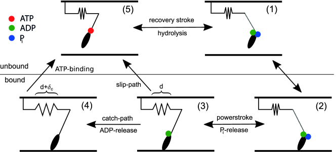
Figure 1: Five-state crossbridge model for myosin II. Motors stochastically cycle through five mechano-chemical states with different lever arm conformations and different combinations of ATP, ADP and P_i bound to the motor head. Rates for transitions between states depend on mechanical load and ATP concentration, and are specific for the myosin II isoform.

II Five-state crossbridge model

Our crossbridge model for the myosin II motor cycle with five mechano-chemical states is sketched in Fig. 1. In the two states above the line myosin II is unbound, while in the three states below it is bound to the actin filament. The reversible transition $(5)\to(1)$ with forward rate $k_{51}$ and reverse rate $k_{15}$ is the recovery stroke. In transition $(1)\to(2)$, myosin II motors reversibly bind to actin with forward rate $k_{12}$ and reverse rate $k_{21}$. The powerstroke $(2)\to(3)$ is driven by a large free energy gain and is very fast (below milliseconds). The forward rate $k_{23}$ is several orders of magnitude larger than the reverse rate $k_{32}$ and here both rates are assumed to be constant Lan and Sun (2005), although in practise they might also show some load-dependance. The powerstroke stretches the elastic neck linker with an effective spring constant $k_{\mathrm{m}}$ by a distance $d$. From state $(3)$, we consider two alternative paths for irreversible unbinding Stam et al. (2015). The regular motor cycle proceeds from $(3)\to(4)$ (catch path). It requires additional lever arm movement by $\delta_{\mathrm{c}}<d$ and is impeded by mechanical load Veigel et al. (2003). This load dependence is described by transition rate $k_{34}=k_{34}^{0}\exp\left(-F_{\mathrm{m}}/F_{\mathrm{c}}\right)$, where $F_{\mathrm{m}}=k_{\mathrm{m}}x$ is the load on a motor with neck linker strain $x$ and $F_{\mathrm{c}}=k_{\mathrm{B}}T/\delta_{\mathrm{c}}$. Because the reverse transition requires binding of ADP, which usually is maintained at very low concentrations, transition $(3)\to(4)$ is considered as irreversible. Unbinding of myosin II from actin in transition $(4)\to(5)$ requires binding of ATP. This is described by the transition rate $k_{45}=k_{\mathrm{T}}\left[\mathrm{ATP}\right]$. Alternatively, motors can unbind directly from state $(3)$ to $(5)$ along the slip path with transition rate $k_{35}=k_{35}^{0}\exp\left(F_{\mathrm{m}}/F_{\mathrm{s}}\right)$, which increases with the load $F_{\mathrm{m}}$. The slip path for unbinding has been demonstrated in single molecule experiments Guo and Guilford (2006). With $k_{34}^{0}\gg k_{35}^{0}$ and $F_{\mathrm{s}}\gg F_{\mathrm{c}}$, it is activated only under large load and prevents stalling of the motor cycle.

Parameter	Symbol	Units	Skeletal	Smooth	NM IIA	NM IIB	References
Transition rates	$k_{12}$	$\text{\,}\mathrm{s}^{-1}$	$40$	$6$	$0.2$	$0.2$	Vilfan and Duke (2003); Walcott et al. (2012); Stam et al. (2015)
	$k_{21}$	$\text{\,}\mathrm{s}^{-1}$	$2$	$2$	$0.004$	$0.004$	Duke (1999); Kovács et al. (2003)
	$k_{23}=k_{23}^{0}\operatorname{e}^{-\frac{E_{\mathrm{pp}}}{2k_{\mathrm{B}}T}}$	$\text{\,}\mathrm{s}^{-1}$	$1.4\cdot 10^{6}$	$1.4\cdot 10^{6}$	$1.4\cdot 10^{6}$	$1.4\cdot 10^{6}$	Vilfan and Duke (2003)
	$k_{32}=k_{32}^{0}\operatorname{e}^{+\frac{E_{\mathrm{pp}}}{2k_{\mathrm{B}}T}}$	$\text{\,}\mathrm{s}^{-1}$	$7\cdot 10^{-1}$	$7\cdot 10^{-1}$	$7\cdot 10^{-1}$	$7\cdot 10^{-1}$	Vilfan and Duke (2003)
	$k_{23}^{0}=k_{32}^{0}$	$\text{\,}\mathrm{s}^{-1}$	$1000$	$1000$	$1000$	$1000$	Vilfan and Duke (2003)
	$k_{34}^{0}/k_{3}^{0}$	$-$	$0.92$	$0.92$	$0.92$	$0.92$	Guo and Guilford (2006); Stam et al. (2015)
	$k_{35}^{0}/k_{3}^{0}$	$-$	$0.08$	$0.08$	$0.08$	$0.08$	Guo and Guilford (2006); Stam et al. (2015)
	$k_{3}^{0}$	$\text{\,}\mathrm{s}^{-1}$	$350$	$18$	$1.71$	$0.35$	Vilfan and Duke (2003); Walcott et al. (2012); Stam et al. (2015)
	$k_{\mathrm{T}}$	$\text{\,}\left\mathrm{missing}{(}\mathrm{s}\usk\mathrm{\SIUnitSymbolMicro}\mathrm{M}\right\mathrm{missing}{)}^{-1}$	$2$	$1.2$	$1.2$	$1.2$	Walcott et al. (2012)
	$k_{51}$	$\text{\,}\mathrm{s}^{-1}$	$100$	$100$	$100$	$100$	Walcott et al. (2012)
	$k_{15}$	$\text{\,}\mathrm{s}^{-1}$	$10$	$10$	$10$	$10$	Walcott et al. (2012)
Powerstroke distances	$d$	$\text{\,}\mathrm{nm}$	$10$	$10$	$5.5$	$5.5$	Walcott et al. (2012); Stam et al. (2015)
	$\delta_{\mathrm{c}}$	$\text{\,}\mathrm{nm}$	$1.86$	$2.60$	$2.5$	$2.5$	Walcott et al. (2012); Stam et al. (2015)
Unbinding forces	$F_{\mathrm{c}}$	$\text{\,}\mathrm{pN}$	$2.23$	$1.59$	$1.66$	$1.66$	Walcott et al. (2012); Stam et al. (2015)
	$F_{\mathrm{s}}$	$\text{\,}\mathrm{pN}$	$13.91$	$9.95$	$10.35$	$10.35$	Walcott et al. (2012); Stam et al. (2015); Guo and Guilford (2006)
Powerstroke bias	$E_{\mathrm{pp}}$	$\text{\,}\mathrm{p}\mathrm{N}\usk\mathrm{n}\mathrm{m}$	$-60$	$-60$	$-60$	$-60$	Vilfan and Duke (2003)
Neck linker elasticity	$k_{\mathrm{m}}$	$\text{\,}\mathrm{pN}\text{\,}{\mathrm{nm}}^{-1}$	$0.3$	$0.3$	$0.7$	$0.7$	Walcott et al. (2012); Stam et al. (2015)
Thermal energy	$k_{\mathrm{B}}T$	$\text{\,}\mathrm{p}\mathrm{N}\usk\mathrm{n}\mathrm{m}$	$4.14$	$4.14$	$4.14$	$4.14$	Vilfan and Duke (2003)
Mobility	$\eta$	$\text{\,}\mathrm{n}\mathrm{m}\mathrm{/}\left\mathrm{missing}{(}\mathrm{s}\usk\mathrm{p}\mathrm{N}\right\mathrm{missing}{)}$	$1000$	$1000$	$1000$	$1000$	Erdmann et al. (2013)
Duty ratio	$\rho$	$-$	$0.1$	$0.25$	$0.1$	$0.36$	$-$

Table 1: Model parameters for different myosin II isoforms as extracted from the literature.

In Tab. 1 we list the molecular parameters and transition rates of our model for four different myosin II isoforms as extracted from the literature. Following our earlier work on myosin II ensembles Erdmann and Schwarz (2012); Erdmann et al. (2013); Albert et al. (2014), the parameters for skeletal muscle myosin II are used as the reference case which here is compared to results for other myosin II isoforms. Parameters for skeletal and smooth muscle myosin II are taken from Ref. Walcott et al. (2012) and for non-muscle myosin IIA and B from Ref. Stam et al. (2015). Parameters not included in those models are supplemented from Refs. Vilfan and Duke (2003); Walcott et al. (2012); Guo and Guilford (2006). It should be noted that literature values for powerstroke distance $d$ and neck linker elasticity $k_{\mathrm{m}}$ are usually effective quantities obtained by fitting procedures and vary significantly even for the same isoform. For skeletal and smooth muscle myosin II, we use the small value $0.3\text{\,}\mathrm{pN}\text{\,}{\mathrm{nm}}^{-1}$ given in Ref. Walcott et al. (2012). For non-muscle myosin IIA and B, on the other hand, we use the larger value $k_{\mathrm{m}}=$0.7\text{\,}\mathrm{pN}\text{\,}{\mathrm{nm}}^{-1}$$ used in Ref. Stam et al. (2015). Parameters in Ref. Walcott et al. (2012) are obtained from fits to laser trap experiments and motility assays for small myosin II ensembles so that compliance of the environment might contribute to the smaller neck linker stiffness. Parameters in Ref. Stam et al. (2015) are based on single molecule experiments. Moreover, the parameters from Ref. Walcott et al. (2012) yield larger values for the single motor duty ratio at vanishing load and large ATP concentration than observed in muscle. The single motor duty ratio $\rho$ describes the probability that a motor is bound to the substrate. For a two-state model, it would be $k_{\rm on}/(k_{\rm on}+k_{\rm off})$. Due to the large powerstroke rate $k_{23}$, the single motor duty ratio for vanishing load and large ATP concentration can be estimated as $\rho\simeq k_{12}/(k_{12}+k_{3}^{0})$ as done in the last line of Tab. 1.

In a myosin II ensemble, $N_{\mathrm{t}}$ individual motors are coupled to the rigid motor filament via their elastic neck linkers. The state of an ensemble is characterized by the mechano-chemical states of all motors and the positions of bound motor heads on the actin filament. For given external load $F_{\mathrm{ext}}$, the position $z_{\mathrm{fil}}$ of the motor filament is adjusted dynamically by the balance of external load and elastic motor forces $F_{\mathrm{m}}=k_{\mathrm{m}}x$ of all bound motors Erdmann et al. (2013). The resulting bound velocity $v_{\mathrm{b}}$ is averaged to give a measure for how well the ensemble is advancing. Although single motors usually step only forward, the filament can also move backward if unbound motors rebind behind the average position of bound motors heads on the substrate. Moreover, due to the small ensemble size, it can happen that all motors are unbound at once. In this case, a different physical process has to take over to determine how fast the ensemble is moving. Here we assume that while the filament is unbound, it is pulled backwards with unbound velocity $v_{\mathrm{u}}=-\eta F_{\mathrm{ext}}$, until a first motor binds through transition $(1)\to(2)$. Due to this important effect, the resulting effective velocity $v_{\mathrm{eff}}$ is smaller than the bound velocity $v_{\mathrm{b}}$. Here we analyze the dynamics of myosin II ensembles numerically using exact stochastic simulations with the Gillespie algorithm. For more details on these procedures, we refer to our earlier work Erdmann and Schwarz (2012); Erdmann et al. (2013); Albert et al. (2014).

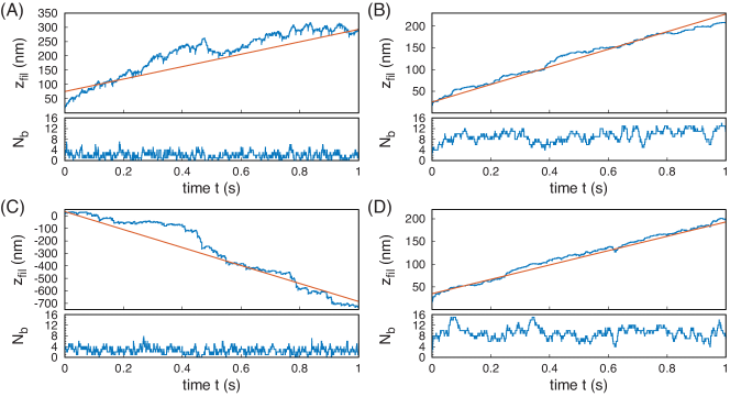
Figure 2: Stochastic trajectories for a skeletal muscle myosin II ensemble of size $N_{\mathrm{t}}=16$. Each trajectory displays the fluctuating number $N_{\mathrm{b}}$ of bound motors (lower panel) and the position $z_{\mathrm{fil}}$ of the motor filament (upper panel) as function of time. The straight lines indicate movement with average effective velocity $\left<v_{\mathrm{eff}}\right>$. Trajectories are shown for small and large values of external load and ATP concentration: $F_{\mathrm{ext}}/N_{\mathrm{t}}=0.2$\text{\,}\mathrm{pN}$$ in (A,B) (top) and $F_{\mathrm{ext}}/N_{\mathrm{t}}=0.5$\text{\,}\mathrm{pN}$$ in (C,D) (bottom); $\left[\mathrm{ATP}\right]=1$\text{\,}\mathrm{m}\mathrm{M}$$ in (A,C) (left) and $\left[\mathrm{ATP}\right]=10$\text{\,}\mathrm{\SIUnitSymbolMicro}\mathrm{M}$$ in (B,D) (right).

III Trajectories

Fig. 2 shows typical stochastic trajectories for a skeletal myosin II minifilament of size $N_{\mathrm{t}}=16$, which is a typical value for the number of active myosin II motor heads in the minifilament ensembles used in motility assays and in the cytoskeleton of non-muscle cells. For each trajectory, lower and upper panels display the fluctuating number $N_{\mathrm{b}}$ of bound motors and the fluctuating position $z_{\mathrm{fil}}$ of the motor filament, respectively. The stochastic trajectory of $z_{\mathrm{fil}}$ is compared to movement with average effective velocity $\left<v_{\mathrm{eff}}\right>$.

In Fig. 2 (A), mechanical load is small while ATP concentration is large and comparable to cellular concentrations. Due to the small single motor duty ratio, the average number of bound motors is small, $\left<N_{\mathrm{b}}\right>\simeq 1.9\ll N_{\mathrm{t}}$, and the ensemble frequently detaches completely. For the small load, both bound and effective velocity are positive, although $\left<v_{\mathrm{eff}}\right>\simeq 220$\text{\,}\mathrm{nm}\text{\,}{\mathrm{s}}^{-1}$$ is significantly smaller than $\left<v_{\mathrm{b}}\right>\simeq 540$\text{\,}\mathrm{nm}\text{\,}{\mathrm{s}}^{-1}$$. Fig. 2 (B) demonstrates the stabilizing effect of decreased ATP concentration. The average number of bound motors increases to $\left<N_{\mathrm{b}}\right>\simeq 8.8$ and ensemble detachment is no longer observed. Bound and effective velocity are therefore identical, $\left<v_{\mathrm{b}}\right>\simeq\left<v_{\mathrm{eff}}\right>\simeq 200$\text{\,}\mathrm{nm}\text{\,}{\mathrm{s}}^{-1}$$, but both are smaller than for large ATP concentration. Fig. 2 (C) demonstrates the stabilizing effect of increased external load at the same high ATP concentration as in (A). The average number of bound motors now is $\left<N_{\mathrm{b}}\right>\simeq 2.6$ and complete detachment occurs less frequently than in (A). Because the high load opposes movement, the ensemble now moves backwards with $\left<v_{\mathrm{b}}\right>\simeq-520$\text{\,}\mathrm{nm}\text{\,}{\mathrm{s}}^{-1}$$ and $\left<v_{\mathrm{eff}}\right>\simeq-720$\text{\,}\mathrm{nm}\text{\,}{\mathrm{s}}^{-1}$$.

Fig. 2 (D) demonstrates the effect of reduced ATP concentration at large external load. Compared to (A), the average number of bound motors is increased to $\left<N_{\mathrm{b}}\right>\simeq 8.8$. As in (B), ensemble detachment does not occur so that bound and effective velocities are identical. In contrast to the case of small load, backward movement observed at large load and large ATP concentration in Fig. 2 (C) is reversed to forward movement with $\left<v_{\mathrm{b}}\right>=\left<v_{\mathrm{eff}}\right>\simeq 160$\text{\,}\mathrm{nm}\text{\,}{\mathrm{s}}^{-1}$>0$. Although motor cycle time is increased by the decreased ATP concentration, load sharing by an increased number of motors leads to larger and eventually positive positional steps per motor cycle. For sufficiently large load, the mechanical effect of load sharing outruns the effect of motor cycle kinetics.

IV Phase diagrams

We now turn to a systematic analysis of the averaged behavior of small myosin II ensembles. Fig. 3 (A) and (B) show average number of bound motors and average bound velocity, respectively, as function of ATP concentration and external load for a small ensemble with skeletal muscle myosin II. For small ATP concentrations, the average number of bound motors shown in Fig. 3 (A) is large and independent of $F_{\mathrm{ext}}$, because the motor cycle is limited by unbinding from rigor state. With increasing ATP concentration, $\left<N_{\mathrm{b}}\right>$ decreases rapidly and becomes load dependent. Above physiological ATP concentration of $\sim 1$\text{\,}\mathrm{m}\mathrm{M}$$, the motor cycle is limited by load dependent rates $k_{34}+k_{35}\ll k_{45}$, thus $\left<N_{\mathrm{b}}\right>$ becomes independent of ATP concentration.

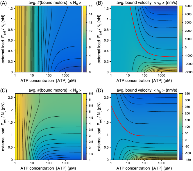
Figure 3: Muscle isoforms. Phase diagrams for (A) the average number $\left<N_{\mathrm{b}}\right>$ of bound motors and (B) the average bound velocity $\left<v_{\mathrm{b}}\right>$ for a skeletal muscle myosin II ensemble of size $N_{\mathrm{t}}=16$ as a function of external load per motor $F_{\mathrm{ext}}/N_{\mathrm{t}}$ and ATP concentration $\left[\mathrm{ATP}\right]$. (C,D) The same for smooth muscle myosin II, but for smaller ensemble size $N_{\mathrm{t}}=8$. The stall force is marked by a thick red line.

Fig. 3 (B) reveals a similar pattern for $\left<v_{\mathrm{b}}\right>$ as for $\left<N_{\mathrm{b}}\right>$, with weak load dependence for small ATP concentrations and weak ATP dependence at high ATP concentrations. However, the behavior of $\left<v_{\mathrm{b}}\right>$ with increasing ATP concentration is more complex than for $\left<N_{\mathrm{b}}\right>$. For very small $F_{\mathrm{ext}}$, $\left<v_{\mathrm{b}}\right>$ increases monotonously with ATP concentration because the motor cycle is accelerated. For larger external load, $\left<v_{\mathrm{b}}\right>$ increases with small ATP concentration but passes through a maximum and decreases with further increasing $\left[\mathrm{ATP}\right]$, because the external load is focused on a decreasing number of bound motors so that the motor cycle leads to backward steps of the ensemble. For ATP concentrations above the physiological level, $\left<v_{\mathrm{b}}\right>$ becomes independent of $\left[\mathrm{ATP}\right]$, but depends strongly on $F_{\mathrm{ext}}$. The upward convex force-velocity relation at constant $\left[\mathrm{ATP}\right]$ corresponds to the Hill relation Hill (1938) and is due to load sharing by an increasing number of bound motors Duke (1999); Erdmann and Schwarz (2012). The average effective velocity $\left<v_{\mathrm{eff}}\right>$ shows a similar behavior as $\left<v_{\mathrm{b}}\right>$ (not shown). Because the boundaries between the different regimes mainly depend on single motor properties, they shift only slightly for larger ensemble size $N_{\mathrm{t}}$ (not shown). The typical level of load which myosin II ensembles can sustain is specified by bound and effective stall forces, $F_{\mathrm{b}}^{0}$ and $F_{\mathrm{eff}}^{0}$, at which average bound and effective velocities vanish, respectively. Marked by the red isoline in Fig. 3 (B), the bound stall force $F_{\mathrm{b}}^{0}$ decreases strongly with increasing ATP concentration. This implies that to achieve forward motion, it is better to work at low ATP concentration. Due to stochastic ensemble detachment, the effective stall force is slightly smaller than $F_{\mathrm{b}}^{0}$ for $\left[\mathrm{ATP}\right]>100$\text{\,}\mathrm{\SIUnitSymbolMicro}\mathrm{M}$$.

Having first discussed skeletal myosin II as a reference case, we next turn to smooth muscle myosin II. As evident from Tab. 1, the most important change in the parameter set for smooth muscle myosin II relative to skeletal muscle myosin II are the small values of the transition rates $k_{3}^{0}$ from post-powerstroke state $(3)$ and the rate $k_{12}$ of binding to the weakly-bound state $(2)$. At vanishing load and large ATP concentration, these rates lead to a single motor duty ratio of $\rho\simeq 0.25$ compared to $\rho\simeq 0.1$ for skeletal muscle myosin II. Therefore, a significantly smaller ensemble size $N_{\mathrm{t}}$ is sufficient to stabilize ensemble attachment.

Fig. 3 (C) and (D) shows the average number of bound motors and the average bound velocity, respectively, of an ensemble of $N_{\mathrm{t}}=8$ smooth muscle myosin II motors as function of ATP concentration and external load. The plots reveal the same qualitative dependence of $\left<N_{\mathrm{b}}\right>$ and $\left<v_{\mathrm{b}}\right>$ on $\left[\mathrm{ATP}\right]$ and $F_{\mathrm{ext}}/N_{\mathrm{t}}$ as for skeletal muscle myosin II. However, the transition from the ATP sensitive regime (at low $\left[\mathrm{ATP}\right]$) to the load sensitive regime (at large $\left[\mathrm{ATP}\right]$) is shifted to smaller ATP concentrations because of the smaller value of $k_{34}+k_{35}$ relative to the rate $k_{45}=k_{\mathrm{T}}\left[\mathrm{ATP}\right]$ of unbinding from rigor state at a given value of $\left[\mathrm{ATP}\right]$. This effect is partially offset by the smaller value of the ATP binding rate $k_{\mathrm{T}}$. At small ATP concentrations, the fraction of bound motors is comparable (although slightly smaller because of the reduced binding rate $k_{12}$) to the case of skeletal muscle myosin II. In the load sensitive regime at large ATP, on the other hand, the average fraction $\left<N_{\mathrm{b}}\right>/N_{\mathrm{t}}$ of bound motors is significantly larger because of the increased single motor duty ratio. Moreover, $\left<N_{\mathrm{b}}\right>/N_{\mathrm{t}}$ increases more strongly with $F_{\mathrm{ext}}/N_{\mathrm{t}}$ (from $\left<N_{\mathrm{b}}\right>/N_{\mathrm{t}}\simeq 0.18$ at $F_{\mathrm{ext}}=0$ to a maximum of $\left<N_{\mathrm{b}}\right>/N_{\mathrm{t}}\simeq 0.52$ at $F_{\mathrm{ext}}/N_{\mathrm{t}}\simeq 2.5$\text{\,}\mathrm{pN}$$), because the force scale $F_{\mathrm{c}}$ for the catch-path is smaller than for skeletal muscle myosin II. For very small ATP concentrations, bound velocity is mainly determined by the slow unbinding from rigor state $(4)$ and becomes comparable for smooth and skeletal muscle myosin II. For large ATP concentrations, bound velocity $\left<v_{\mathrm{b}}\right>$ is reduced by a factor $\sim 10$ because of the reduced rates $k_{34}+k_{35}$ and $k_{12}$. Due to the larger fraction of bound motors sharing the external load, however, $\left<v_{\mathrm{b}}\right>$ reduces more slowly with increasing load and the stall force per bond, $F_{\mathrm{b}}^{0}/N_{\mathrm{t}}$, is larger than for skeletal muscle myosin II (note the larger force scale in Fig. 3 (D) compared to Fig. 3 (B)).

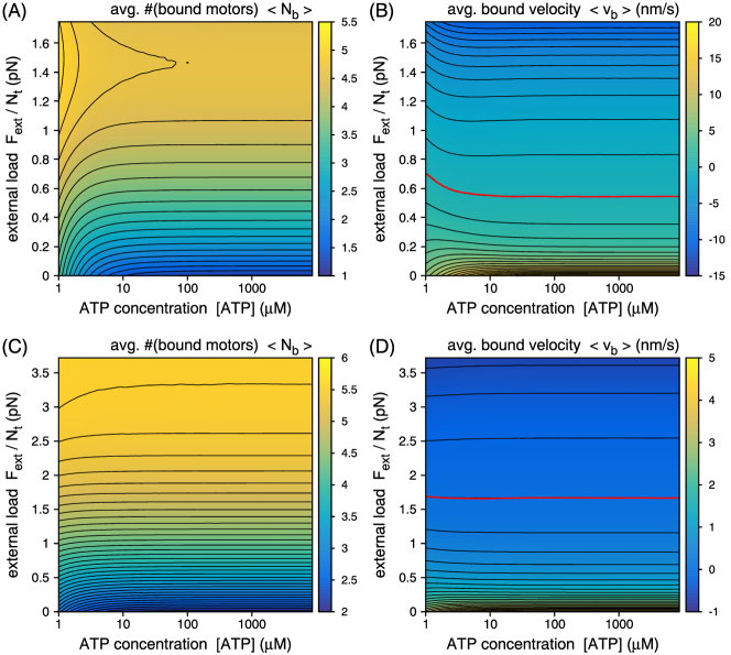
Figure 4: Non-muscle isoforms. Phase diagrams for (A) the average number $\left<N_{\mathrm{b}}\right>$ of bound motors and (B) the average bound velocity $\left<v_{\mathrm{b}}\right>$ for a non-muscle myosin IIA ensemble of size $N_{\mathrm{t}}=16$ as a function of external load per motor $F_{\mathrm{ext}}/N_{\mathrm{t}}$ and ATP concentration $\left[\mathrm{ATP}\right]$. (C,D) The same for non-muscle myosin IIB, but for smaller ensemble size $N_{\mathrm{t}}=8$. The stall force is marked by a thick red line.

We next discuss the cases of the non-muscle myosin II isoforms. As in the case of skeletal and smooth muscle myosin II, mechanical parameters for the two non-muscle isoforms of myosin II are very similar. Compared to the muscle isoforms, however, neck linker stiffness $k_{\mathrm{m}}$ is larger and powerstroke length $d$ is smaller for the non-muscle isoforms. Dynamics of non-muscle myosin IIA and B is characterized by very small values of binding rate $k_{12}$ and transition rate $k_{34}+k_{35}$, which slow down the motor cycle. The values of the transition rates result in single motor duty ratios at vanishing load and large ATP concentration of $\rho\simeq 0.1$ for non-muscle myosin IIA and $\rho\simeq 0.36$ for non-muscle myosin IIB.

Fig. 4 (A) and (B) show load and ATP dependence of $\left<N_{\mathrm{b}}\right>$ and $\left<v_{\mathrm{b}}\right>$, respectively, for an ensemble of non-muscle myosin IIA with $N_{\mathrm{t}}=16$, so that it can be compared well with skeletal muscle myosin II from Fig. 3 (A) and (B). In contrast to the cases of the muscle isoforms, $\left<N_{\mathrm{b}}\right>$ and $\left<v_{\mathrm{b}}\right>$ are essentially independent of ATP concentration due to the very small value of the load-dependent rate $k_{34}+k_{35}$ relative to the ATP dependent rate $k_{45}$. Thus $\left<N_{\mathrm{b}}\right>$ and $\left<v_{\mathrm{b}}\right>$ are load dependent over the full range of ATP concentrations. The average number of bound motors is similar to the case of skeletal muscle myosin II in the load dependent regime at high ATP concentration. The average bound velocity for non-muscle myosin IIA is very small compared to the case of skeletal muscle myosin II, but shows the same Hill-type decrease with increasing load. The bound stall force $F_{\mathrm{b}}^{0}$ is essentially independent of ATP concentration.

For non-muscle myosin IIB, transition rate $k_{34}+k_{35}$ from the post-powerstroke state as given in Tab. 1 is further reduced relative to non-muscle myosin IIA, compare Tab. 1. As a consequence, non-muscle myosin IIB has a higher single motor duty ratio $\rho\simeq 0.36$, but the motor cycle is even slower than for non-muscle myosin IIA. This relation of the non-muscle isoform is similar to the relation of slow smooth muscle myosin II with large duty ratio to the fast skeletal muscle myosin II with a small duty ratio.

Fig. 4 (C) and (D) shows the average number of bound motors and average bound velocity of an ensemble of non-muscle myosin IIB motors as function of ATP concentration and external load. Here we choose $N_{\mathrm{t}}=8$ in order to compare with the smooth muscle case from Fig. 3 (C) and (D). The transition to the ATP sensitive regime is shifted to even smaller ATP concentrations than for non-muscle myosin IIA. As expected from the larger single motor duty ratio, the average fraction $\left<N_{\mathrm{b}}\right>/N_{\mathrm{t}}$ of bound motors is larger than for non-muscle myosin IIA or smooth muscle myosin II in the load sensitive regime at large $\left[\mathrm{ATP}\right]$. Due to the smaller value of $k_{34}+k_{35}$ the average bound velocity $\left<v_{\mathrm{b}}\right>$ is further reduced. Because of the large fraction of bound motors and the large value of neck linker stiffness, however, the bound stall force per motor is significantly larger than for non-muscle myosin IIA or smooth muscle myosin II.

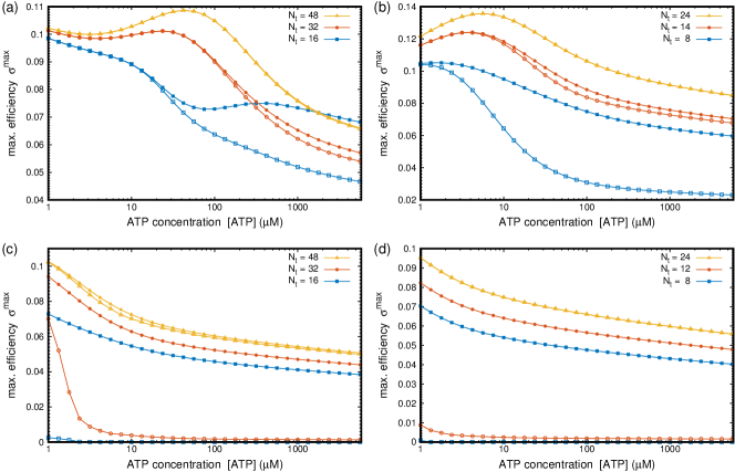
Figure 5: Maximal efficiency $\sigma^{\mathrm{m}}_{\mathrm{b}}$ and $\sigma^{\mathrm{m}}_{\mathrm{eff}}$ for the bound movement (solid symbols) and the effective movement (open symbols) as function of ATP concentration. (A) Skeletal muscle myosin II ensembles with sizes $N_{\mathrm{t}}=16$, $24$ and $48$. (B) Smooth muscle myosin II ensembles with sizes $N_{\mathrm{t}}=8$, $14$ and $24$. (C) Non-muscle myosin IIA ensembles with same sizes as in (A). (D) Non-muscle myosin IIB ensembles with sizes $N_{\mathrm{t}}=8$, $12$ and $24$.

V Ensemble efficiency

The observation that decreasing ATP concentration can increase the average bound velocity of a myosin II ensemble means that the efficiency of movement can be increased by a reduced energy supply. To investigate this interesting point in more detail, we define the effective thermodynamic efficiency for bound and effective movement as the ratio of power output and input Parmeggiani et al. (1999); Schmiedl and Seifert (2008); Zimmermann and Seifert (2012):

$$\sigma_{\mathrm{b}}=\frac{F_{\mathrm{ext}}\left<v_{\mathrm{b}}\right>}{J_{\mathrm{ATP}}\Delta G}\quad\text{and}\quad\sigma_{\mathrm{eff}}=\frac{F_{\mathrm{ext}}\left<v_{\mathrm{eff}}\right>}{J_{\mathrm{ATP}}\Delta G}\,.$$ (1)

$J_{\mathrm{ATP}}$ is the average flux through the motor cycle, in which ATP is converted to ADP and P_i, and $\Delta G$ is the Gibbs free energy released during ATP hydrolysis. For convenience, we calculate the flux for the load-independent transition $(1)\to(2)$ as $J_{\mathrm{ATP}}=N_{\mathrm{t}}(p_{1}k_{12}-p_{2}k_{21})$, where $p_{i}$ is the stationary probability to be in state $i$, thereby neglecting small corrections that might result from load dependance. $\Delta G$ depends on ATP concentration through $\Delta G=\Delta G_{0}-k_{\mathrm{B}}T\ln\left(\left[\mathrm{ATP}\right]M/\left[\mathrm{ADP}\right]\left[\mathrm{P_{i}}\right]\right)$ Howard (2001), where concentrations are measured in units of $M$ and $\Delta G_{0}=-13\ k_{\mathrm{B}}T$, $\left[\mathrm{ADP}\right]=10$\text{\,}\mathrm{\SIUnitSymbolMicro}\mathrm{M}$$ and $\left[\mathrm{P_{i}}\right]=1$\text{\,}\mathrm{m}\mathrm{M}$$ under physiological conditions.

Fig. 5 (A) shows the maximal efficiencies $\sigma^{\mathrm{m}}_{\mathrm{b}}$ and $\sigma^{\mathrm{m}}_{\mathrm{eff}}$ for bound and effective movement as function of ATP concentration for different skeletal muscle myosin II ensemble sizes. The larger ensemble size, the smaller are the differences between bound and effective efficiencies. For small ATP concentrations, $\sigma^{\mathrm{m}}_{\mathrm{b}}$ and $\sigma^{\mathrm{m}}_{\mathrm{eff}}$ depend weakly on $\left[\mathrm{ATP}\right]$ because both flux $J_{\mathrm{ATP}}$ and power output approach zero for $\left[\mathrm{ATP}\right]\to 0$. For larger $N_{\mathrm{t}}$, $\sigma^{\mathrm{m}}_{\mathrm{b}}$ and $\sigma^{\mathrm{m}}_{\mathrm{eff}}$ display a maximum before decreasing with increasing ATP concentrations. Above physiological ATP concentrations, $\sigma^{\mathrm{m}}_{\mathrm{b}}$ and $\sigma^{\mathrm{m}}_{\mathrm{b}}$ continue to decrease slowly because the maximal power output plateaus and energy consumption $J_{\mathrm{ATP}}\Delta G$ continues to increase. Behavior of $\sigma^{\mathrm{m}}_{\mathrm{b}}$ and $\sigma^{\mathrm{m}}_{\mathrm{eff}}$ confirms that reducing energy supply increases ensemble efficiency, in particular for ATP concentrations just below the physiological level.

The maximal efficiencies $\sigma^{\mathrm{m}}_{\mathrm{b}}$ and $\sigma^{\mathrm{m}}_{\mathrm{eff}}$ plotted in Fig. 5 (B) for ensembles of smooth muscle myosin II show the same qualitative dependence on $\left[\mathrm{ATP}\right]$ as observed for skeletal muscle myosin II. Because the transition to the ATP sensitive regime occurs at smaller values of the ATP concentration, the maxima of $\sigma^{\mathrm{m}}_{\mathrm{b}}$ and $\sigma^{\mathrm{m}}_{\mathrm{eff}}$ are also shifted to smaller ATP concentrations. For the smallest ensemble size $N_{\mathrm{t}}=8$, the difference of effective and bound efficiencies is larger than for skeletal muscle myosin II and is observed at smaller ATP concentrations. Because of the smaller bound velocity and the reduced rebinding rate, ensemble detachment reduces the effective velocity more strongly than for skeletal muscle myosin II. Although ensemble velocity is smaller for smooth muscle myosin II, the efficiency is quantitatively similar to the case of skeletal muscle myosin II, because the reduced power output is compensated by the reduced rate of ATP consumption.

Fig. 5 (C) shows the maximal efficiencies $\sigma^{\mathrm{m}}_{\mathrm{b}}$ and $\sigma^{\mathrm{m}}_{\mathrm{eff}}$ for non-muscle myosin IIA. For bound movement $\sigma^{\mathrm{m}}_{\mathrm{b}}$ shows a significant decrease with increasing ATP concentration only for extremely small values of $\left[\mathrm{ATP}\right]$. Maximal efficiency $\sigma^{\mathrm{m}}_{\mathrm{eff}}$ of effective movement deviates strongly from $\sigma^{\mathrm{m}}_{\mathrm{b}}$ and drops to zero for the smaller ensembles as a consequence of ensemble detachment. Although ensemble detachment does not occur more frequently than for skeletal muscle myosin II, effective velocity is reduced more strongly because of the smaller rebinding rate $k_{12}$ and the large unbound velocity relative to $\left<v_{\mathrm{b}}\right>$.

Fig. 5 (D) plots the maximal efficiencies of bound and effective ensemble movement for non-muscle myosin IIB ensembles. The maximal efficiency $\sigma^{\mathrm{m}}_{\mathrm{b}}$ of the bound ensemble movement shows a very weak decrease with increasing ATP concentration similar to non-muscle myosin IIA and comparable to skeletal and smooth muscle myosin II at large values of $\left[\mathrm{ATP}\right]$. Although bound ensemble velocity is very small for non-muscle myosin IIB, the efficiency is quantitatively similar to the case of skeletal muscle myosin II, because the reduced power output is compensated by the reduced rate of ATP consumption. As for non-muscle myosin IIA, the maximal efficiency $\sigma^{\mathrm{m}}_{\mathrm{eff}}$ of effective movement deviates strongly from $\sigma^{\mathrm{m}}_{\mathrm{b}}$ and drops to zero for the smaller ensembles as a consequence of ensemble detachment. Because of the smaller rebinding rate $k_{12}$ and the large unbound velocity $v_{\mathrm{u}}$ relative to $\left<v_{\mathrm{b}}\right>$, the effective velocity becomes negative for very small external load on the ensemble.

VI Discussion

Using a detailed five-state crossbridge model for the myosin II motor cycle, we have systematically analyzed the influence of mechanical load and ATP concentration on the stochastic dynamics of small myosin II ensembles for different isoforms of myosin II. Because load and ATP dependence are described by sequential transitions in the crossbridge cycle, influence of load becomes more pronounced with increasing ATP concentration.

For the muscle isoforms we observe two distinct regimes for myosin II ensemble dynamics: an ATP sensitive regime with weak load dependence at small ATP concentrations, and a mechano-sensitive regime at large ATP concentrations. For the non-muscle isoforms, which cycle much slower than their muscle counterparts, only the mechano-sensitive regime is observed. Transition to an ATP sensitive regime would require ATP concentrations well below the level commonly used in motility assays or actomyosin gels. We speculate that ATP concentrations in cells might be locally more variable than formerly appreciated Imamura et al. (2009); Nakano et al. (2011); Ando et al. (2012), for example during phases of fast actin polymerization and strong actomyosin contraction in migrating cells, but that the non-muscle isoforms are buffered from this effect by their low ATP sensitivity as demonstrated in Fig. 4 compared to Fig. 3.

Ensemble movement results from the interplay of motor cycle kinetics and ensemble mechanics which are both affected by ATP concentration. Decreasing ATP concentration from the mechano-sensitive regime at near vanishing load stabilizes ensembles but decreases velocity. This is known from skeletal muscle and was investigated before in motility assays Walcott et al. (2012). Here we also have shown the effects for decreasing ATP concentration at large load, as it might occur in the cytoskeleton of non-muscle cells and in actomyosin gels, and have found that ensemble velocity can in fact increase, because the collective effect of load sharing by an increasing number of bound motors outruns increased motor cycle time. We find that maximal efficiency increases with decreasing ATP concentration, similar to ratchet models for single motors Parmeggiani et al. (1999). For the small myosin II ensembles, however, we find that in our model the effective thermodynamic efficiency is rather low (typically $\sigma^{\mathrm{m}}_{\mathrm{b}}$ is below $0.1$).

Our results for ensemble efficiency are in stark contrast to the much higher values for single motors, like e.g. the F₁-ATPase Zimmermann and Seifert (2012). They are also in stark contrast to the values for skeletal muscle, which has been measured to be of the order of $0.3$ Whipp and Wasserman (1969). There are several reasons why efficiency is low in our model. We first note that motors mechanically work against each other and that they dissipate elastic energy during unbinding. We also note that for small ensembles, our results are strongly shaped by the physical process that takes over during times of unbinding. For simplicity, here we have used hydrodynamic slip during times of unbinding, but it would be interesting to consider also other physical processes in this context. Interestingly, we also observed that in our model, efficiency can be as high as $0.5$ when optimizing parameter values (mainly by increasing $k_{\mathrm{m}}$ while keeping ATP flux effectively constant by adjusting other parameters). This indicates that our results depend sensitively on parameter values, which here have been chosen from the literature as listed in Tab. 1.

Finally, our work shows that one has to be careful when drawing conclusions on cellular contractility from reconstituted actomyosin gels. Here one often uses skeletal or smooth muscle myosin II and reduces ATP concentrations to stabilize the system Soares e Silva et al. (2011); Köhler et al. (2011); Murrell and Gardel (2012); Ideses et al. (2013); Linsmeier et al. (2016). Our analysis shows that decreasing ATP concentrations has the desired effect of increased contractility for the muscle myosin II isoforms. However, it also shows that the same would not work for non-muscle myosin II isoforms, because they are less sensitive to changes in ATP concentrations, and that the resulting numbers for bound motors and contraction velocities might be quite different.