Hydrodynamic interactions between nearby slender filaments

Abstract

Cellular biology abound with filaments interacting through fluids, from intracellular microtubules, to rotating flagella and beating cilia. While previous work has demonstrated the complexity of capturing nonlocal hydrodynamic interactions between moving filaments, the problem remains difficult theoretically. We show here that when filaments are closer to each other than their relevant length scale, the integration of hydrodynamic interactions can be approximately carried out analytically. This leads to a set of simplified local equations, illustrated on a simple model of two interacting filaments, which can be used to tackle theoretically a range of problems in biology and physics.

While one tends to think of biological cells as stubby, their environment is in fact rich with filamentous structures. Inside cells, polymeric filaments of microtubules, actin, and intermediate filaments fill the eukaryotic cytoplasm Alberts et al. (2007) and provide it with its mechanical structure Boal (2002). Outside cells, the motion of flagella and cilia allows cells to generate propulsive forces Berg and Anderson (1973); Brennen and Winet (1977); Lauga and Powers (2009) and induces flows critical to human health Sleigh et al. (1988); Fauci and Dillon (2006).

In all cases, these biological filaments are immersed in a viscous fluid in which they move at low Reynolds number, be it due to their polymerisation, to fluctuations and thermal forces, or to the action of molecular motors Bray (2000). At low Reynolds number, the flows induced locally by the motion of filaments relative to a background fluid have a slow spatial decay as $\sim 1/r$ Lighthill (1975); Leal (2007). In situations where filaments are close to each other, we thus expect nonlocal hydrodynamic interactions to be important Goldstein et al. (2016).

Integrating long-ranged hydrodynamic interactions between filaments has long been recognised as a challenging problem, and one where the theoretical approach has consisted of either full numerical simulations or very simplified analysis. A variety of computational methods have been developed to tackle it including slender-body theory Johnson (1980); Gueron and Liron (1993); Tornberg and Shelley (2004), boundary elements to implement boundary integral formulations Kanehl and Ishikawa (2014), the immersed boundary method Lim and Peskin (2012); Yang et al. (2008a), regularised flow singularities Flores et al. (2005) and particle-based methods Yang et al. (2010); Reigh et al. (2012).

While these computational approaches allow to address complex geometries and dynamics, the difficulty of integrating long-range hydrodynamic interactions has prevented analytical approaches from providing insight beyond simplified setups. The two most common approaches in biophysics consist in replacing the dynamics in three dimensions by a two-dimensional problem for which the analysis may be easier to carry out Taylor (1951); Elfring and Lauga (2009), or by focusing on far-field hydrodynamic interactions and ignoring the geometrical details of near-field hydrodynamics, a popular approach to study synchronisation of flagella and cilia Vilfan and Julicher (2006); Guirao and Joanny (2007); Niedermayer et al. (2008); Uchida and Golestanian (2010); Golestanian et al. (2011); Friedrich and Jülicher (2012); Bennett and Golestanian (2013).

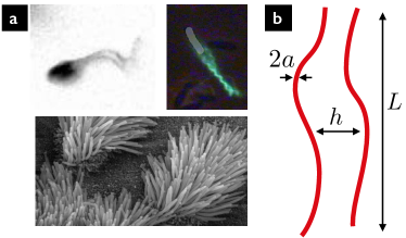
Figure 1: (a) Examples where nearby filaments interact through a viscous fluid (clockwise from top left): two spermatozoa synchronising their flagella (reprinted with permission from Yang, Elgeti & Gompper, Physical Review E, 78, 061903, 2008 Yang et al. (2008b); copyright 2008, American Physical Society); flagellar filaments of peritrichous bacteria during swarming (reprinted with permission from Turner, Zhang, Darnton & Berg, Journal of Bacteriology, 192, 3259–3267, 2010 Turner et al. (2010); copyright 2010, American Society for Microbiology); epithelium cilia (courtesy of C. Daghlian, Wikimedia Commons). (b) Prototypical setup: two slender filaments of length $L$ and radius $a$ at a typical distance $h$ from each other.

In realistic biological situations, three-dimensional filaments are not far from each other, but in fact are often found in the opposite, near-field, limit where their separation distance is much smaller than their length. This is illustrated in Fig. 1a with three examples relevant to cell motility: synchronising flagella of spermatozoa; bundle of bacterial flagellar filaments; epithelium cilia. In order to capture the dynamics of these interacting filaments, new analytical tools are thus required.

In this paper, we show that analytical progress can be achieved by taking advantage of a separation of length scales. A generic two-filament setup (as in Fig. 1b) is characterised by three length scales: the filament radius, $a$; the separation distance between the filaments, $h$; and the filament length, $L$. While far-field studies focus on the limit $h\gg\{L,a\}$, many biological situations are in the opposite near-field limit, for example in the case of waving cilia arrays Blake and Sleigh (1974), for which $\{a,h\}\ll L$, i.e. slender filaments close to each other compared to their typical size. We show here that in the special case where $a\ll h$, i.e. for filaments thinner than any another other length scale in the problem, the hydrodynamic interactions between the filaments can be analytically integrated out, leading to a set of simplified local equations valid in the limit $a\ll h\ll L$. Our results, illustrated on a simple model of two interacting rigid filaments, will allow to tackle theoretically a range of problems in biology and physics.

Consider the two filaments in Fig. 1b, numbered #1 and #2. Denote the location of the centerline to filament $i$ as $\mathbf{r}^{(i)}(s,t)$ where $s$ is the arclength, and let $\mathbf{t}^{(i)}(s)={\partial\mathbf{r}^{(i)}}/{\partial s}$ be its unit tangent. In order to compute the hydrodynamic forces on the filaments, we exploit the two assumed separations of scales, $a\ll h\ll L$. We first note that the limit $a\ll L$ implies that the filaments are slender. Furthermore, since the displacements of the filaments are at most on the order of their separation distance, $h$, their typical curvature, denoted $\kappa$, is at most of order $\kappa\sim h/L^{2}$. Since we assume the limit $h\ll L$, this means that we have always $\kappa h\ll 1$ and $\kappa L\ll 1$, and the filaments undergo long-wavelength deformation. In that case, resistive-force theory may be used to calculate the hydrodynamic force densities on each filament Gray and Hancock (1955); Cox (1970); Lighthill (1975). Denoting the force densities $\mathbf{f}^{(1)}$ and $\mathbf{f}^{(2)}$, resistive-force theory states that they are proportional to the local velocity of the filament relative the background fluid i.e.

$$\mathbf{f}^{(1)}=-\left(\xi_{\perp}\mathbf{I}+(\xi_{\parallel}-\xi_{\perp})\mathbf{t}^{(1)}\mathbf{t}^{(1)}\right)\cdot\left(\frac{\partial\mathbf{r}^{(1)}}{\partial t}-\mathbf{v}^{(2)\to(1)}\right),\\ \mathbf{f}^{(2)}=-\left(\xi_{\perp}\mathbf{I}+(\xi_{\parallel}-\xi_{\perp})\mathbf{t}^{(2)}\mathbf{t}^{(2)}\right)\cdot\left(\frac{\partial\mathbf{r}^{(2)}}{\partial t}-\mathbf{v}^{(1)\to(2)}\right),$$ (1)

where all fields are implicitly functions of $s$ and $t$ and where $\xi_{\perp}$ and $\xi_{\parallel}$ are the drag coefficients for motion in the direction perpendicular and parallel to its local tangent Gray and Hancock (1955); Cox (1970); Lighthill (1975). We compute below the hydrodynamic force density acting on filament #1, the other one being deduced by symmetry. In Eq. 1, the term $\mathbf{v}^{(2)\to(1)}$ denotes the flow induced by the motion of filament $2$ near filament $1$: it represents the effect of hydrodynamic interactions and the goal of this paper is to show how to calculate its value. As filament #2 undergoes in general both rotational and translational motion, we split $\mathbf{v}^{(2)\to(1)}$ into the flows induced by local moments, $\mathbf{v}_{M}^{(2)\to(1)}$ (rotation), and those induced by local forces, $\mathbf{v}_{F}^{(2)\to(1)}$ (translation). We then write $\mathbf{v}^{(2)\to(1)}=\mathbf{v}_{M}^{(2)\to(1)}+\mathbf{v}_{F}^{(2)\to(1)}$, and calculate the values of each term in the long-wavelength limit, $h\ll L$.

In order to simplify the presentation, we focus in detail on the derivation of the first velocity term, $\mathbf{v}^{(2)\to(1)}_{M}$, induced by the rotational motion of filament #2, while the value of $\mathbf{v}_{F}^{(2)\to(1)}$ is computed along similar lines (see below). Note that while $\mathbf{v}^{(2)\to(1)}_{M}$ is exactly zero for non-rotating filaments, e.g. in the case of the planar waving flagella of spermatozoa, it will be important in other situations involving rotation, e.g. the dynamics of bacterial flagellar filaments. Since $a\ll h$, the flow may be described by a superposition of flow singularities. If $\mathbf{m}^{(2)}$ denotes the hydrodynamic torque density acting on filament #2, the flow is given as a line of integral of rotlets (or point torques) as Batchelor (1970)

$$\mathbf{v}_{M}^{(2)\to(1)}(s)=\int_{0}^{L}\frac{-\mathbf{m}^{(2)}(s^{\prime})}{8\pi\mu}\times\frac{\mathbf{R}(s,s^{\prime})}{R(s,s^{\prime})^{3}}{\rm d}s^{\prime},$$ (2)

where $s$ and $s^{\prime}$ are the arclengths along filaments $\#1$ and $\#2$ and $\mathbf{R}(s,s^{\prime})=\mathbf{r}^{(1)}(s)-\mathbf{r}^{(2)}(s^{\prime})$ is the relative position vector with magnitude $R$ (all quantities are implicit functions of time). If filament #2 rotates relative to the background fluid with rotation rate $\omega^{(2)}(s^{\prime})$ then it is a classical result that

$$\mathbf{m}^{(2)}(s^{\prime})=-\xi_{r}\omega^{(2)}(s^{\prime})\mathbf{t}^{(2)}(s^{\prime}),$$ (3)

where the resistance coefficient in rotation is $\xi_{r}=4\pi\mu a^{2}$.

We nondimensionalize lengths by $L$, leading to two dimensionless numbers: the filament aspect ratio, $\epsilon_{a}=a/L$, and the distance-to-size ratio, $\epsilon_{h}=h/L$. Times are non-dimensionalised by a relevant, problem-specific time scale $T$. The integral from Eq. 2 becomes then in dimensionless form

$$\bar{\mathbf{v}}_{M}^{(2)\to(1)}(\bar{s})=\frac{\epsilon_{a}^{2}}{2}\int_{0}^{1}\bar{\omega}(\bar{s}^{\prime})^{(2)}\mathbf{t}^{(2)}(\bar{s}^{\prime})\times\frac{\bar{\mathbf{R}}(\bar{s},\bar{s}^{\prime})}{\bar{R}(\bar{s},\bar{s}^{\prime})^{3}}{\rm d}\bar{s}^{\prime},$$ (4)

and we drop the bars for notation convenience.

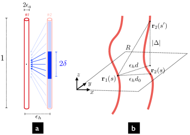
Figure 2: (a) Illustration of method to compute hydrodynamic interactions. The integration region is split into a local region of size $2\delta$ and a non-local region where the separation of lengths $\epsilon_{h}\ll\delta\ll 1$ may be exploited to compute the flow separately. (b) Geometric relations between $d$, $d_{0}$ and $R$: $R$ is the distance between points on two filaments, $\epsilon_{h}d$ the projection in $x-y$ plane and $\epsilon_{h}d_{0}$ the local separation distance.

Since we are in the long-wavelength limit, it is natural to use cartesian coordinates (Fig. 2). We denote by $\mathbf{e}_{z}$ the unit vector along the mean direction of the (approximately) parallel filaments and describe the instantaneous geometry of each filament as $\mathbf{r}^{(i)}(t,s^{(i)})=\left[\epsilon_{h}x^{(i)}(t,s^{(i)}),\epsilon_{h}y^{(i)}(t,s^{(i)}),s^{(i)}\right]$ where $s^{(1)}\equiv s$ and $s^{(2)}\equiv s^{\prime}$. Introducing the notation $\Delta=s-s^{\prime}$ and the planar vector $\mathbf{d}(s;s^{\prime})=[x^{(1)}(s)-x^{(2)}(s^{\prime}),y^{(1)}(s)-y^{(2)}(s^{\prime}),0]$ of magnitude $d=|\mathbf{d}|$, then the relative position vector $\mathbf{R}$ is written by separating the direction along and perpendicular to the filaments as $\mathbf{R}=\Delta\mathbf{e}_{z}+\epsilon_{h}\mathbf{d},$ with magnitude $R=\left(\Delta^{2}+\epsilon_{h}^{2}d^{2}\right)^{1/2}$.

The schematic representation of how the integration is performed is shown in Fig. 2a with detailed notation in Fig. 2b. Our method is inspired by a classical calculation due to Lighthill where, in order to describe the flow induced by the motion of a single filament, he separated the flow induced by point singularities into local and nonlocal terms using an intermediate length scale on which the filament was still slender but almost straight Lighthill (1975). We introduce an intermediate length scale $\delta$ satisfying $\epsilon_{h}\ll\delta\ll 1$ and split the integration into two regions: (1) a nonlocal region, $|\Delta|\geq\delta$, where the distance between two points on the filaments is dominated by $R\sim|\Delta|$ since $\epsilon_{h}\ll\delta$ (resulting velocity denoted $\mathbf{v}^{{\rm NL}}$); and (2) a local region where $|\Delta|\leq\delta$, and for which in the limit $\delta\ll 1$ we can approximate $R\sim\left(\Delta^{2}+\epsilon_{h}^{2}d_{0}^{2}\right)^{1/2}$ where $d_{0}$ is the local filament-filament distance $d_{0}(s)=d(s;s^{\prime}=s)$ (resulting velocity denoted $\mathbf{v}^{{\rm L}}$). The final result, sum of $\mathbf{v}^{{\rm NL}}$ and $\mathbf{v}^{{\rm L}}$, should then be independent of the value of $\delta$.

Changing the variable of integration in Eq. 4 to $\Delta=s-s^{\prime}$, the non-local contribution to the integral is given by

$$\mathbf{v}_{M}^{{\rm NL}}=\frac{\epsilon_{a}^{2}}{2}\left(\int_{s-1}^{-\delta}+\int_{\delta}^{s}\right)\left[\omega^{(2)}\mathbf{t}^{(2)}\right]_{(s-\Delta)}\times\frac{\mathbf{R}}{R^{3}}{\rm d}\Delta.$$ (5)

Since $|\Delta|\geq\delta$ and $\epsilon_{h}\ll\delta$, we have $R(s;s-\Delta)\approx|\Delta|$. Writing $\mathbf{R}=\Delta\mathbf{e}_{z}+\epsilon_{h}\mathbf{d}(s;s-\Delta)$ and $\mathbf{t}^{(2)}(s-\Delta)=\mathbf{e}_{z}+\epsilon_{h}\mathbf{t}_{\perp}(s-\Delta)$ where $\displaystyle\mathbf{t}_{\perp}(s-\Delta)=\left(\frac{\partial{x^{(2)}}}{\partial{s^{\prime}}},\frac{\partial{y^{(2)}}}{\partial{s^{\prime}}},0\right)\big{|}_{s^{\prime}=s-\Delta}$, the integrand from Eq. 5 is given by

$$\epsilon_{h}\omega^{(2)}(s-\Delta)[\mathbf{e}_{z}\times\mathbf{d}(s;s-\Delta)+\mathbf{t}_{\perp}(s-\Delta)\times\Delta\mathbf{e}_{z}]\frac{1}{|\Delta|^{3}}\cdot$$ (6)

The leading-order term in Eq. 6 diverges as $1/\Delta^{3}$ in the limit $\delta\to 0$, leading to a final asymptotic integral as

$$\mathbf{v}_{M}^{{\rm NL}}=\frac{\epsilon_{a}^{2}\epsilon_{h}}{2}\left(\int_{-\delta}^{s-1}\!\!\!+\int_{\delta}^{s}\right)\omega^{(2)}(s-\Delta)\mathbf{e}_{z}\times\mathbf{d}(s;s-\Delta)\frac{{\rm d}\Delta}{\Delta^{3}}\cdot$$ (7)

In the limit where $\delta\to 0$, the result in Eq. 7 diverges and is dominated by the behavior of the integrand near the boundary, i.e. $\Delta=0$. Calling $\mathbf{d}_{0}$ the local direction between the filaments perpendicular to their long axis, i.e. $\mathbf{d}_{0}=\mathbf{d}(s;s)$ (Fig. 2b), we obtain in the limit $\delta\to 0$

$$\mathbf{v}_{M}^{{\rm NL}}=\frac{\epsilon_{a}^{2}\epsilon_{h}}{2\delta^{2}}\omega^{(2)}(s)\mathbf{e}_{z}\times\mathbf{d}_{0},$$ (8)

at leading order.

Next we consider the local integration where we have

$$\mathbf{v}_{M}^{{\rm L}}=\frac{\epsilon_{a}^{2}}{2}\int_{-\delta}^{\delta}\omega^{(2)}(s-\Delta)\mathbf{t}^{(2)}(s-\Delta)\times\frac{\mathbf{R}}{R^{3}}d\Delta.$$ (9)

In the local region, we can Taylor-expand $\omega^{(2)}$ and $\mathbf{d}$ around $\Delta=0$ (i.e. around $s^{\prime}=s$) as

$$\left(\begin{array}[]{c}\displaystyle\omega(s-\Delta)^{(2)}\\ \displaystyle\mathbf{d}(s-\Delta)\end{array}\right)=\left(\begin{array}[]{c}\displaystyle\omega(s)^{(2)}\\ \displaystyle\mathbf{d}(s)\end{array}\right)+\Delta\left(\begin{array}[]{c}\omega^{(2)}_{0\Delta}\\ \mathbf{d}_{0\Delta}\end{array}\right)+O(\Delta^{2}),$$ (10)

where, under the long-wavelength approximation, the derivatives $\omega^{(2)}_{0\Delta}$ and $\mathbf{d}_{0\Delta}$ are of order one (i.e. the geometry and the rotation of the filaments vary on the length scale $L$). In that case, each term in the integrand can be expanded and we get at leading order that only the local values of the rotation rate, $\omega^{(2)}(s)$, and the force, $\mathbf{f}^{(2)}(s)$, enter the problem, with a local flow given by

$$\mathbf{v}_{M}^{{\rm L}}=\frac{\epsilon_{a}^{2}\epsilon_{h}}{2}\omega^{(2)}(s)\int_{-\delta}^{\delta}\frac{\mathbf{e}_{z}\times\mathbf{d}_{0}}{(\Delta^{2}+\epsilon_{h}^{2}d_{0}^{2})^{\frac{3}{2}}}{\rm d}\Delta,$$ (11)

which may be evaluated analytically with an asymptotic expression given by

$$\mathbf{v}_{M}^{{\rm L}}=\frac{\epsilon_{a}^{2}\epsilon_{h}}{2}\omega^{(2)}(s)\,\mathbf{e}_{z}\times\mathbf{d}_{0}\left(\frac{2}{\epsilon_{h}^{2}d_{0}^{2}}-\frac{1}{\delta^{2}}\right).$$ (12)

Adding up Eq. 8 and 12, we obtain the final flow induced by filament #2, which is independent of the value of $\delta$, given at leading-order by

$$\mathbf{v}_{M}^{(2)\to(1)}=\frac{\epsilon_{a}^{2}}{\epsilon_{h}d_{0}^{2}}\omega^{(2)}(s)\mathbf{e}_{z}\times\mathbf{d}_{0}.$$ (13)

A similar approach may be used to evaluate the second velocity term, $\mathbf{v}^{(2)\to(1)}_{F}$, induced by the forcing of filament #2 on the fluid. In that case, the flow is given by a line integral of stokeslet singularities (point forces) as

$$\mathbf{v}_{F}^{(2)\to(1)}(s)=\int_{0}^{L}\frac{-\mathbf{f}^{(2)}(s^{\prime})}{8\pi\mu}\cdot\left(\frac{\mathbf{I}}{R}+\frac{\mathbf{R}\mathbf{R}}{R^{3}}\right){\rm d}s^{\prime},$$ (14)

where $\mathbf{I}$ is the identity tensor and $\mathbf{f}^{(2)}$ the force density acting on filament #2. One notable difference between Eq. 2 and Eq. 14 is that the integrand in Eq. 2 is known explicitly (filament rotation), whereas that in Eq. 14 has in it the quantity we are trying to determine, specifically the unknown force density, $\mathbf{f}^{(2)}$. We can however proceed as above as long as $\mathbf{f}^{(2)}$ varies on the length scale $L$, and similarly for the other filament, so that the resulting velocities in Eq. 1 will lead to a linear system to invert to determine both $\mathbf{f}^{(1)}$ and $\mathbf{f}^{(2)}$. After nondimensionalising force densities by $8\pi\mu L/T$, the nonlocal contribution of the integral in Eq. 14 is written as

$$\mathbf{v}_{F}^{{\rm NL}}=-\left(\int_{s-1}^{-\delta}+\int_{\delta}^{s}\right)\left(\frac{\mathbf{I}}{R}+\frac{\mathbf{R}\mathbf{R}}{R^{3}}\right)\cdot\mathbf{f}^{(2)}(s-\Delta){\rm d}\Delta,$$ (15)

whose evaluation at leading-order value is given by the logarithmic term

$$\mathbf{v}_{F}^{{\rm NL}}=2(\ln\delta)(\mathbf{I}+\mathbf{e}_{z}\mathbf{e}_{z})\cdot\mathbf{f}^{(2)}(s).$$ (16)

Similarly, the local portion of the integral, written as

$$\mathbf{v}_{F}^{{\rm L}}=-\int_{-\delta}^{\delta}\left(\frac{\mathbf{I}}{R}+\frac{\mathbf{R}\mathbf{R}}{R^{3}}\right)\cdot\mathbf{f}^{(2)}{\rm d}\Delta,$$ (17)

can be Taylor-expanded and exactly integrated to lead to the local logarithmic dependence

$$\mathbf{v}_{F}^{{\rm L}}=2\ln\left(\frac{\epsilon_{h}d_{0}}{\delta}\right)(\mathbf{I}+\mathbf{e}_{z}\mathbf{e}_{z})\cdot\mathbf{f}^{(2)}(s).$$ (18)

Adding Eq. 16 and 18 we obtain the final force term as

$$\mathbf{v}_{F}^{(2)\to(1)}=2\ln\left({\epsilon_{h}d_{0}}\right)(\mathbf{I}+\mathbf{e}_{z}\mathbf{e}_{z})\cdot\mathbf{f}^{(2)}(s),$$ (19)

for the velocity induced by the unknown force density.

Returning to dimensional quantities Eqs. 13-19 can be written as

$$\mathbf{v}_{M}^{(2)\to(1)}=\left(\frac{a}{h(s)}\right)^{2}\omega^{(2)}(s)\mathbf{e}_{z}\times{\bf h}{(s)},$$ (20)

$$\mathbf{v}_{F}^{(2)\to(1)}=\frac{1}{4\pi\mu}\ln\left(\frac{h(s)}{L}\right)(\mathbf{I}+\mathbf{e}_{z}\mathbf{e}_{z})\cdot\mathbf{f}^{(2)}(s),$$ (21)

where ${\bf h}(s)$ is the dimensional local vector between the filaments, i.e. ${\bf h}(s)=\mathbf{r}_{1}(s)-\mathbf{r}_{2}(s)$, and $h(s)$ its norm.

The results in Eqs. 20-21, together with Eq. 1 are the main new results of this paper. They provide a linear, local relationship between the force density on each filament ($\mathbf{f}^{(i)}$) and the kinematics of their motion ($\omega^{(j)}$ and $\partial\mathbf{r}^{(k)}/\partial t$). As a remark, we note that one is not allowed to formally take the limit $h\to 0$ or $h\to\infty$ in Eqs. 20-21, as both violate the limit $a\ll h\ll L$ in which these formulae were derived.

For planar motion ($\omega^{(j)}=0$ for $j=1,2$), the algebra simplifies further. In Eq. 1, since $h\ll L$, the tangent vectors are $\mathbf{t}=\mathbf{e}_{z}$ at leading order in $h/L$ and since $\xi_{\perp}\approx 2\xi_{\parallel}$ Lighthill (1975) we have for each filament

$$\xi_{\perp}\mathbf{I}+(\xi_{\parallel}-\xi_{\perp})\mathbf{t}\mathbf{t}\approx\xi_{\perp}\left(\mathbf{I}-\frac{1}{2}\mathbf{e}_{z}\mathbf{e}_{z}\right)\equiv\bf J,$$ (22)

so that on each filament $i$ we have the dynamic balance

$$\mathbf{f}^{(i)}(s,t)-{\bf J}\cdot\mathbf{v}^{(j)\to(i)}=-{\bf J}\cdot\frac{\partial\mathbf{r}^{(i)}}{\partial t},$$ (23)

with $j\neq i$. Given the tensorial operator appearing in Eq. 21, we have to evaluate

$$\left(\mathbf{I}-\frac{1}{2}\mathbf{e}_{z}\mathbf{e}_{z}\right)\cdot(\mathbf{I}+\mathbf{e}_{z}\mathbf{e}_{z})=\mathbf{I},$$ (24)

and we further note that ${\xi_{\perp}}/{4\pi\mu}\approx{1}/{\ln(1/\epsilon_{a})}$ Lighthill (1975). As a result, Eq. 23 simplifies for each filament to

$$\mathbf{f}^{(i)}(s,t)+\frac{\ln({h(s,t)}/{L})}{\ln(a/L)}\mathbf{f}^{(j)}(s,t)=-{\bf J}\cdot\frac{\partial\mathbf{r}^{(i)}}{\partial t},$$ (25)

with $j\neq i$. Defining $\lambda(s,t)\equiv{\ln({h(s,t)}/{L})}/{\ln(a/L)}$ and $\Lambda(s,t)\equiv 1-\lambda^{2}(s,t)$ (note that $\Lambda>0$ since $a<h$), this linear system can be inverted by hand and we obtain the analytical formula for the force density $\mathbf{f}^{(i)}(s,t)$ acting on filament $i$ as

$$\mathbf{f}^{(i)}(s,t)=-\frac{1}{\Lambda(s,t)}{\bf J}\cdot\left(\frac{\partial\mathbf{r}^{(i)}}{\partial t}-\lambda(s,t)\frac{\partial\mathbf{r}^{(j)}}{\partial t}\right).$$ (26)

We now illustrate predictions of our theory on a simple model of two rigid filaments undergoing planar motion, and compare with numerical slender-body simulations. Consider two straight coplanar filaments of radius $a$, length $L$ with centerlines located at $[0,\epsilon y_{1}(z,t),z]$ and $[0,h_{0}+\epsilon y_{2}(z,t),z]$. Assume for simplicity small amplitude motion $\epsilon\ll 1$ and let us use our results to calculate the force density in the $y$ direction, $f^{(i)}=\mathbf{f}^{(i)}\cdot\mathbf{e}_{y}$, in powers of the amplitude ($f^{(i)}=\epsilon f_{1}^{(i)}+\epsilon^{2}f_{2}^{(i)}+...$) in the limit $a\ll h_{0}\ll L$. Writing $h=h_{0}+\epsilon h_{1}$, a Taylor expansion gives

$$\ln\left({h}/{L}\right)=\ln\left({h_{0}}/{L}\right)+\epsilon{h_{1}}/{h_{0}}+O(\epsilon^{2}),$$ (27)

which we use to evaluate Eq. 26 at order $\epsilon$, leading to

$$f_{1}^{(i)}=\frac{\xi_{\perp}}{1-[\ln(h_{0}/L)/\ln(a/L)]^{2}}\left(\frac{\ln(h_{0}/L)}{\ln(a/L)}\frac{\partial y^{(j)}}{\partial t}-\frac{\partial y^{(i)}}{\partial t}\right).$$ (28)

At order $\epsilon^{2}$, Eq. 25 becomes

$$f_{2}^{(i)}+\frac{\ln({h_{0}}/{L})}{\ln(a/L)}f_{2}^{(j)}=-\frac{h_{1}}{h_{0}\ln(a/L)}f_{1}^{(j)},$$ (29)

Assuming that both $y_{1}$ and $y_{2}$ are periodic in time on the same period, then a time-average of Eq. 29 using Eq. 28 leads to identical mean force densities along both filaments as $\big{\langle}f_{2}^{(1)}\big{\rangle}=\big{\langle}f_{2}^{(2)}\big{\rangle}=f_{2}(s)$, where

$$f_{2}(s)=\frac{\xi_{\perp}\ln(a/L)}{2h_{0}[\ln(h_{0}/L)+\ln(a/L)]^{2}}\bigg{\langle}y_{-}\frac{\partial y_{+}}{\partial t}\bigg{\rangle},$$ (30)

with $y_{+}\equiv y^{(1)}+y^{(2)}$ and $y_{-}\equiv y^{(2)}-y^{(1)}$.

For illustration purposes, let us assume that the first filament undergoes sinusoidal rigid-body motion of the form $y_{1}(t)={\cal R}(\sum_{n}\ell_{n}\exp in\omega t)$ while the second filament has the same motion with a phase difference $\phi$, i.e. $y_{2}(t)=y_{1}(t+\phi)$. Our theory, Eq. 30, predicts that the two-rod system will pump the fluid by exerting a net force on it, $F$, of magnitude

$$F_{2}=\frac{4\pi\mu\omega L}{2h_{0}[\ln(h_{0}/L)+\ln(a/L)]^{2}}\sum_{n}n|\ell_{n}|^{2}\sin(n\phi)\cdot$$ (31)

Clearly Eq. 31 predicts zero net force for in-phase ($\phi=0$) and out-of-phase ($\phi=\pi$) motion and thus an optimal phase difference between the two filaments exits.

We test in Fig. 3 this theoretical prediction against a numerical implementation of nonlocal slender-body appropriate for interactions Johnson (1980); Tornberg and Gustavsson (2006) in the case $n=1$. We numerically solve for the force distribution along each filament using a Galerkin method based on Legendre polynomials. The net force on each filament is then computed at 15 equidistant points within a period, and the mean force calculated. While the theoretical approach (Eq. 31) was derived only asymptotically in the limit where $a/h\to 0$ and $h/L\to 0$ we see that even when these parameters are not asymptotically small (here $a/h=0.25$ and $h/L=0.1$), the theoretical prediction (solid line) is able to capture the computational results (dashed line and symbols) with good approximation. In contrast, far-field predictions are off by more than two orders of magnitude.

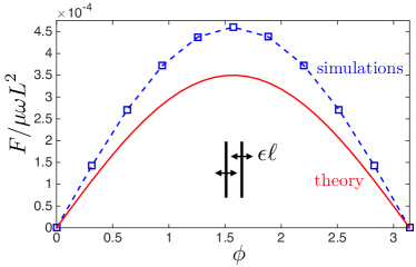
Figure 3: Net force induced on the fluid by a two-rod pump, $F/\mu\omega L^{2}$, as a function of the phase difference, $\phi$, between the rods. Dashed line and symbols: slender-body theory simulations; Solid line: theory (Eq. 31). The dimensionless distance between the rods is $h/L=0.1$, their aspect ratio $a/L=0.025$ (so that $a/h=0.25$) and the motion amplitude is $\epsilon\ell=h/10$.

In summary, we have used an asymptotic method to compute the hydrodynamic interactions between nearby filaments undergoing arbitrary rotation and translation. The key ingredient allowing the calculation to be carried out is to exploit the separation of length scales $a\ll h\ll L$ which enables a representation of the flow as a superposition of fundamental singularities whose strengths vary only on long wavelengths compared to the separation between the filaments. While the work above was derived only in the case of filaments with main directions parallel to each other, future work with be required to generalise the results to the case of non-parallel filaments; we speculate that the “local” aspect of the final equation is likely to involve the point on each filament which is nearest to the other.

Like any other asymptotic derivation, a crucial question in our work is that of the magnitude of the error (i.e. the order of the next-order terms). To fix ideas, consider first a single filament undergoing planar deformation with a centerline described by $[x,y(x,t)]$. The classical formula for the leading-order force density, $\mathbf{f}$, on the filament is $\mathbf{f}=-(\xi_{\perp}\partial y/\partial t)\mathbf{e}_{y}$, with (i) logarithmic corrections in the aspect ratio of the filament from next-order terms beyond resistive-force theory, i.e. relative error $O(1/\ln(L/a))$ Cox (1970) and (ii) algebraic corrections in the typical slope of the filament, i.e. relative error $O(h/L)$ due to the difference between the true instantaneous geometry of the filament and its mean direction Lauga and Powers (2009). The same relative errors apply to our current work. Additional errors arise in our work near the ends of the filaments. Specifically, in order for the non-local integrations to be carried out near the ends of the filaments, the arclength $s$ needs to satisfy $h\ll\min(s,L-s)$, with logarithmically (resp. algebraically) small relative errors in $h/\min(s,L-s)$ from filament translation (resp. rotation). Physically, this logarithmic accuracy of local hydrodynamics is the equivalent to that of resistive-force theory but extended to multiple filaments. The portion of the filament with an admissible arclength $s$ satisfying $\min(s,L-s)\gg h$ is of size $L-2s_{0}$, with $s_{0}\gg h$. Since we are in the limit $h\ll L$, the geometric mean $s_{0}=\sqrt{hL}$ satisfies the intermediate limit $L\gg s_{0}\gg h$. As a consequence, our results are able to provide the value of the hydrodynamic force density on the majority of the filaments, namely at least a portion of size $L-2\sqrt{hL}$.

We finally point out that while the addition of higher-order flow singularities than rotlet and stokeslets along each filament would improve the analysis, the resulting additional terms would decay spatially algebraically and faster than the terms in Eqs. 20-21, which provide thus the leading-order contribution in the limit $a\ll h\ll L$.

The framework developed in this paper will allow to address theoretically a number of problems in the biomechanics of filaments where nonlocal hydrodynamic interactions may be integrated out analytically for example in cytoskeletal mechanics, hydrodynamic interactions and cellular propulsion, beyond the classical, complementary, far-field approach. For example, two particular problems in the realm of biological synchronisation Goldstein et al. (2016) could be tackled: the requirements for attraction and synchronisation between the rotating helical flagellar filaments of bacteria Kim and Powers (2004); Reichert and Stark (2005) and the generation of metachronal waves in cilia arrays Brennen and Winet (1977); Guirao and Joanny (2007); Niedermayer et al. (2008).

Our results should also be applicable to a broad range of problems in physical sciences where slender bodies interact through a viscous fluid, such as liquid crystals. As an example, a set of recent measurements showed strong interactions between living organisms and a liquid crystal Zhou et al. (2014), a situation which could be addressed using our framework.

References

- Alberts et al. (2007) B. Alberts, A. Johnson, J. Lewis, M. Raff, K. Roberts, and P. Walter, Molecular Biology of the Cell, Fifth Edition (Garland Science, New York, NY, 2007).
- Boal (2002) D. Boal, Mechanics of the cell (Cambridge Univ. Press., Cambridge, U.K., 2002).
- Berg and Anderson (1973) H. C. Berg and R. A. Anderson, Nature 245, 380 (1973).
- Brennen and Winet (1977) C. Brennen and H. Winet, Annu. Rev. Fluid Mech. 9, 339 (1977).
- Lauga and Powers (2009) E. Lauga and T. R. Powers, Rep. Prog. Phys. 72, 096601 (2009).
- Sleigh et al. (1988) M. A. Sleigh, J. R. Blake, and N. Liron, Am. Rev. Resp. Dis. 137, 726 (1988).
- Fauci and Dillon (2006) L. J. Fauci and R. Dillon, Ann. Rev. Fluid Mech. 38, 371 (2006).
- Bray (2000) D. Bray, Cell Movements (Garland Publishing, New York, NY, 2000).
- Lighthill (1975) J. Lighthill, Mathematical Biofluiddynamics (SIAM, Philadelphia, 1975).
- Leal (2007) L. G. Leal, Advanced Transport Phenomena: Fluid Mechanics and Convective Transport Processes (Cambridge University Press, Cambridge, UK, 2007).
- Goldstein et al. (2016) R. E. Goldstein, E. Lauga, A. I. Pesci, and M. R. Proctor, Phys. Rev. Fluids. 1, 073201 (2016).
- Johnson (1980) R. E. Johnson, J. Fluid Mech. 99, 411 (1980).
- Gueron and Liron (1993) S. Gueron and N. Liron, Biophys. J. 65, 499 (1993).
- Tornberg and Shelley (2004) A.-K. Tornberg and M. J. Shelley, J Comput Phys 196, 8 (2004).
- Kanehl and Ishikawa (2014) P. Kanehl and T. Ishikawa, Phys. Rev. E 89, 042704 (2014).
- Lim and Peskin (2012) S. Lim and C. S. Peskin, Phys. Rev. E 85, 036307 (2012).
- Yang et al. (2008a) X. Yang, R. H. Dillon, and L. J. Fauci, Bull. Math. Biol. 70, 1192 (2008a).
- Flores et al. (2005) H. Flores, E. Lobaton, S. Mendez-Diez, S. Tlupova, and R. Cortez, Bulletin Math. Biol. 67, 137 (2005).
- Yang et al. (2010) Y. Yang, V. Marceau, and G. Gompper, Phys. Rev. E 82, 031904 (2010).
- Reigh et al. (2012) S. Y. Reigh, R. G. Winkler, and G. Gompper, Soft Matt. 8, 4363 (2012).
- Taylor (1951) G. I. Taylor, Proc. R. Soc. A 209, 447 (1951).
- Elfring and Lauga (2009) G. Elfring and E. Lauga, Phys. Rev. Lett. 103, 088101 (2009).
- Vilfan and Julicher (2006) A. Vilfan and F. Julicher, Phys. Rev. Lett. 96, 058102 (2006).
- Guirao and Joanny (2007) B. Guirao and J. F. Joanny, Biophys. J. 92, 1900 (2007).
- Niedermayer et al. (2008) T. Niedermayer, B. Eckhardt, and P. Lenz, Chaos 18, 037128 (2008).
- Uchida and Golestanian (2010) N. Uchida and R. Golestanian, Phys. Rev. Lett. 104, 178103 (2010).
- Golestanian et al. (2011) R. Golestanian, J. M. Yeomans, and N. Uchida, Soft Matter 7, 3074 (2011).
- Friedrich and Jülicher (2012) B. M. Friedrich and F. Jülicher, Phys. Rev. Lett. 109, 138102 (2012).
- Bennett and Golestanian (2013) R. R. Bennett and R. Golestanian, Phys. Rev. Lett. 110, 148102 (2013).
- Yang et al. (2008b) Y. Yang, J. Elgeti, and G. Gompper, Phys. Rev. E 78, 061903 (2008b).
- Turner et al. (2010) L. Turner, R. Zhang, N. C. Darnton, and H. C. Berg, J. Bacteriol. 192, 3259 (2010).
- Blake and Sleigh (1974) J. R. Blake and M. A. Sleigh, Biol. Rev. Camb. Phil. Soc. 49, 85 (1974).
- Gray and Hancock (1955) J. Gray and G. J. Hancock, J. Exp. Biol. 32, 802 (1955).
- Cox (1970) R. G. Cox, J. Fluid Mech. 44, 791 (1970).
- Batchelor (1970) G. K. Batchelor, J. Fluid Mech. 41, 545 (1970).
- Tornberg and Gustavsson (2006) A.-K. Tornberg and K. Gustavsson, J. Comp. Phys. 215, 172 (2006).
- Kim and Powers (2004) M. Kim and T. R. Powers, Physical Review E 69, 061910 (2004).
- Reichert and Stark (2005) M. Reichert and H. Stark, The European Physical Journal E 17, 493 (2005).
- Zhou et al. (2014) S. Zhou, S. Sokolov, O. D. Lavrentovich, and I. S. Aranson, Proc. Natl. Acad. Sci. U.S.A. 111, 1265 (2014).