Non-Equilibrium Markov State Modeling of the Globule-Stretch Transition

Abstract

We describe a systematic approach to construct coarse-grained Markov state models from molecular dynamics data of systems driven into a non-equilibrium steady state. We apply this method to study the globule-stretch transition of a single tethered model polymer in shear flow. The folding/unfolding rates of the coarse-grained model agree with the original detailed model. We demonstrate that the folding/unfolding proceeds through the same narrow region of configuration space but along different cycles.

I Introduction

Computer simulations have developed into a powerful tool to predict and optimize material properties. However, even given the ever increasing computational power, relevant time and length scales, in particular for biological and synthetic macromolecules Karplus and McCammon (2002); Kamerlin et al. (2011), will remain prohibitively long for fully atomistic simulations, and multiscale methods are crucial to make progress. While structure-based coarse-graining Müller-Plathe (2002) has been quite successful Harmandaris and Kremer (2009); Salerno et al. (2016), challenges remain like transferability (e.g., from bulk to surfaces), and in particular the correct treatment (or a posteriori deduction) of the materials dynamical properties through the coarse-grained dynamics. For the latter, Markov state models (MSMs) Noé and Fischer (2008); Noé et al. (2009); Bowman et al. (2011); Prinz et al. (2011) have been used successfully to tackle the evolution of large proteins towards their native state, bridging the gap from molecular dynamics on nanoseconds to folding on milliseconds Dobson (2003); Noé (2015). The dynamics of MSMs is a discrete-time master equation with transition probabilities obey detailed balance on a network of long-lived (metastable) mesostates.

Here we describe a systematic approach to construct MSMs with dynamics that break detailed balance. We employ this method to study a model polymer in shear flow. The rheology of dilute flexible polymers has been studied extensively due to their fundamental and practical relevance Larson (2005). Examples include biomolecules such as the von Willebrand factor in blood plasma and DNA in steady shear flow Smith et al. (1999). The shear drag can overcome the entropic forces favoring coiled or globular configurations and stretch the polymers, which might be a continuous or even discontinuous transition De Gennes (1974). Motion of DNA tethered to a planar surface has been described as cyclic in experiments Doyle et al. (2000) and computer simulations Delgado-Buscalioni (2006); Zhang et al. (2009).

Driving a system away from thermal equilibrium implies a non-vanishing entropy production. In a steady state, this entropy is produced exclusively in cycles since there are no sources and sinks for the probability. This poses novel challenges for constructing coarse-grained models in non-equilibrium, which only very recently have been begun to be addressed Wang and Schütte (2015); Koltai et al. (2016); Pellegrini et al. (2016). Reducing the complexity by removing states implies a reduced entropy production, which severely influences dynamical properties and fluctuations Puglisi et al. (2010). In Ref. 22, we have introduced non-equilibrium Markov state modeling (NE-MSM) performing the coarse-graining in cycle space instead of collecting configurations in metastable basins as for conventional MSM. The analog of these basins are now communities of cycles with similar properties. The coarse-graining procedure preserves the entropy production of these communities, which makes our approach consistent with stochastic thermodynamics Seifert (2012).

II Model

We study a single model polymer with $N=50$ beads in shear flow inspired by Ref. 24. We employ Brownian dynamics (BD) simulations with

$$\dot{\mathbf{r}}_{k}=-\nabla_{k}U+\mathbf{v}(\mathbf{r}_{k})+\boldsymbol{\eta}_{k}(t)$$ (1)

for the bead positions $\mathbf{r}_{k}=(x_{k},y_{k},z_{k})^{T}$, where $\mathbf{v}(\mathbf{r})$ represents the shear flow. Interactions with solvent particles are modeled by a random force with correlations $\langle\eta_{k}^{\alpha}(t)\eta_{l}^{\beta}(t^{\prime})\rangle=2\delta_{kl}\delta^{\alpha\beta}\delta(t-t^{\prime})$, where upper indices label vector components. The potential energy $U=U_{\text{nb}}+U_{\text{b}}$ is split into the non-bonded short-ranged Lennard-Jones pair potentials $U_{\text{nb}}=\varepsilon_{\text{LJ}}\sum_{k<l}[r_{k,l}^{-12}-2r_{k,l}^{-6}]$ and bonds $U_{\text{b}}=\frac{\kappa}{2}\sum_{k=1}^{N-1}(r_{k+1,k}-1)^{2}$ that connect the nearest neighboring beads. Here, $r_{k,l}$ is the distance between the $k$-th and $l$-th bead, $\varepsilon_{\text{LJ}}=2.3$ determines the strength of the non-bonded potential, and $\kappa=100$ is the effective spring constant. All quantities have been non-dimensionalized by rescaling lengths with the bead diameter $\sigma$ and timescales with the characteristic monomer diffusion time $\sigma^{2}/(4D_{0})$. Numerical values for the strain rate $\dot{\gamma}$ thus correspond to the Weissenberg number.

The polymer is driven into a non-equilibrium steady state through simple shear flow. While some scaling relations depend on hydrodynamic interactions Alexander-Katz et al. (2006); Winkler (2006), the qualitative behavior of the cyclic motion does not and in the following we neglect hydrodynamic interactions. As flow profile we choose

$$\mathbf{v}(\mathbf{r})=\dot{\gamma}(z-z_{\text{c}})\mathbf{e}_{x},$$ (2)

where $\dot{\gamma}$ is the strain rate and $z_{\text{c}}$ is the $z$ component of the center of mass of the polymer. We found that this shift of the flow stabilizes the globular and stretched configurations as it increases the effective barrier for folding/unfolding and thus leads to a better separation between globular and extended states. Qualitatively, the same effect would be expected when including hydrodynamic interactions with the wall. Our conclusions do not depend on this detail. The polymer is grafted onto a repulsive planar surface (the $x$-$y$ plane with $z=0$) by fixing the position of the first bead to $\mathbf{r}_{1}=(0,0,0.5)$. Although simplified, this model reproduces the cyclic dynamics found in experiments Doyle et al. (2000).

A reasonable order parameter describing the folding and unfolding of the polymer is the relative end-to-end distance $R_{\text{ee}}\equiv|x_{0}-x_{N}|/N$, where $R_{\text{ee}}=1$ corresponds to a straight line of touching beads. We perform BD simulations for multiple values of $\dot{\gamma}$, see Fig. 1. We find different behaviors of $\langle R_{\text{ee}}\rangle$ that we categorize into three regimes. For $\dot{\gamma}\lesssim 1$ the polymer remains collapsed, while for $\dot{\gamma}\gtrsim 2.2$ it is dominantly found in elongated conformations. For intermediate strain rates the polymer exhibits transitions between globular and elongated conformations, which was also found in similar simulations for free polymers Alexander-Katz et al. (2006) and grafted polymers Lemak et al. (1998); Delgado-Buscalioni (2006) under shear. The exemplary time series for $\dot{\gamma}=1.6$ in the inset of Fig. 1 shows a clear separation of both states with random lifetimes and fast transitions. The average folding time $t_{\text{fold}}\approx 3000$ is much larger than the intrinsic Rouse time $t_{\text{R}}=N^{2}/(2\pi^{2}\kappa)\sim 1$ of the polymer.

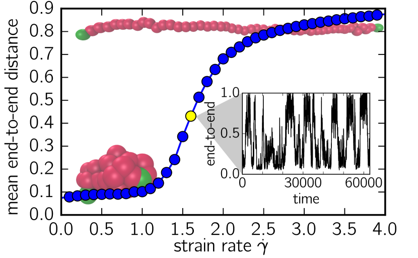
Figure 1: Mean end-to-end distance $\langle R_{\text{ee}}\rangle$ as a function of strain rate $\dot{\gamma}$. For $\dot{\gamma}=1.6$ (yellow/bright circle) the inset shows an exemplary time series. Also shown are two snapshots for the globule (bottom) and extended polymer (top).

III Theory

Our goal is to construct a dynamically consistent NE-MSM with as few discrete states as possible. Every discrete state $i$ is a set of $N$ particle positions, which we collect in the vector $\mathbf{R}_{i}\equiv(\mathbf{r}_{k})$ with $3N$ entries. These states, or centroids, represent discrete volumes of configuration space, i.e., many configurations with slightly different positions. Following Ref. 22, the outline of the algorithm is as follows: The first step is to generate many (specifically $M=500$) centroids using the BD simulation data as input employing a spatial clustering algorithm (for technical details, see Ref. 9 and appendix A). From the counting matrix of transitions in the BD data we construct an approximate Markov process and identify cycles. The crucial step is to group cycles into communities (i.e., clusters of cycles with similar properties defined through suitable order parameters) and determine one cycle representative for each community. In the actual coarse-graining, only representatives and the states that they visit are retained. The final step is then to rescale the Markov dynamics so that it preserves the entropy production of every community as well as the total entropy production.

Entropy production arises from non-vanishing probability currents $J^{i}_{j}\equiv\Phi^{i}_{j}-\Phi^{j}_{i}$ with probability fluxes $\Phi^{i}_{j}$ along transitions $i\to j$. In thermal equilibrium the condition of detailed balance holds, $\Phi^{i}_{j}=\Phi^{j}_{i}$, which implies zero currents. The mean entropy production rate Altaner et al. (2012); Knoch and Speck (2015) is

$$\dot{S}=\sum_{ij}\Phi^{i}_{j}A^{i}_{j}=\frac{1}{2}\sum_{ij}J^{i}_{j}A^{i}_{j}$$ (3)

with affinities $A^{i}_{j}\equiv\log{\Phi^{i}_{j}}-\log{\Phi^{j}_{i}}$.

III.1 Cycle decomposition

In a steady state, Kirchhoff’s law implies that probability flows in cycles. A cycle $\alpha=(i_{1}\to i_{2}\to\cdots\to i_{1})$ is defined as an ordered set of states, at the end of which the starting state is reached again and all other states are visited exactly once. Cycles that differ only in the cyclic permutation of their states are considered identical. We extend the concept of affinities to cycles, yielding the cycle affinities $A_{\alpha}\equiv\sum_{(i\to j)\in\alpha}A^{i}_{j}$, where the sum is over all edges along cycle $\alpha$. Traversing a full cycle, the entropy produced equals the cycle affinity. Graph theoretical results allow us to decompose the probability fluxes Kalpazidou (2007); Knoch and Speck (2015); Altaner et al. (2012)

$$\Phi^{i}_{j}=\sum_{\alpha\ni(i\to j)}\varphi_{\alpha}$$ (4)

into cycle fluxes with non-negative weights $\varphi_{\alpha}\geqslant 0$. The summation is over all cycles $\alpha$ that include the edge $(i\to j)\in\alpha$. The number of cycles quickly becomes very large. Here we employ the algorithm introduced in Ref. 22 and summarized in appendix B to efficiently determine a subset of cycles with non-vanishing weights $\varphi_{\alpha}>0$. These cycles have non-negative cycle affinities (and thus entropy production), which makes our approach conceptually different from the well-known Schnakenberg theory Schnakenberg (1976). Inserting Eq. (4) into Eq. (3), we obtain $\dot{S}=\sum_{\alpha}\varphi_{\alpha}A_{\alpha}$, which clearly shows that all entropy production is encoded in cycles.

III.2 Cycle communities

At this point we have determined all entropy-producing cycles. To make progress, we now need to find similarities between cycles. One approach is to consider the connectivity between cycles Altaner et al. (2012); Conrad et al. (2015); Knoch and Speck (2015). For the globule-stretch transition, we found this approach to be less suitable since it groups cycles that are located in different parts of configuration space . Instead, here we describe an alternative, general method to reduce the complexity of the high-dimensional configuration space to a few variables based on the topology of cycles. As our main tool, we perform a principal component analysis (PCA) Jolliffe (2002), which is an orthogonal linear transformation returning the eigenvectors (the principal components) and eigenvalues of the covariance matrix of the centroid positions. The principal component $\mathbf{C}^{(1)}$ corresponding to the largest eigenvalue coincides with the direction in configuration space exhibiting the largest variance; in the present case it already accounts for $\approx 96$% of the observed variance. In Fig. 2 the normalized projections $c^{(n)}_{i}\equiv\mathbf{R}_{i}\cdot\mathbf{C}^{(n)}/\mathcal{N}$ of centroids onto first and second principal component are plotted, where the normalization $\mathcal{N}$ ensures that $c^{(1)}_{i}\in[-1,1]$. Centroids with small (negative) values for $c^{(1)}_{i}$ correspond to globular configurations (they contribute little to the observed variance of positions), large (positive) values correspond to stretched configurations. The second component indicates the variance within these states. Both globular and stretched configurations show larger fluctuations while the intermediate states with $c^{(1)}_{i}\sim 0$ exhibit less fluctuations. Hence, the PCA reproduces the expected, typical picture of two basins with intermediate transition states.

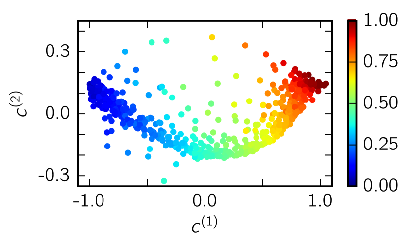
Figure 2: Configuration space ($\dot{\gamma}=1.6$). Scatter plot of the normalized projections of all centroids onto the two largest principal components. Colors indicate the end-to-end distance $R_{\text{ee}}$.

Going back to cycles, we now define two variables: (i) the cycle centers

$$x_{\alpha}\equiv\left(\frac{1}{|\alpha|}\sum_{i\in\alpha}\mathbf{R}_{i}\right)\cdot\mathbf{C}^{(1)}$$ (5)

with $|\alpha|$ the number of centroids in cycle $\alpha$ and (ii) the cycle diameters

$$d_{\alpha}\equiv\max_{i,j\in\alpha}\left\{|c^{(1)}_{i}-c^{(1)}_{j}|\right\}.$$ (6)

The set of points $(x_{\alpha},d_{\alpha})$ is plotted in Fig. 3a, where every point now represents a single cycle. These points are clearly not random. Many cycles have a small diameter $d_{\alpha}$ but different cycle centers. We identify these cycles as local because the centroids $i\in\alpha$ in these cycles have similar $c^{(1)}_{i}$ and thus belong to a compact region in configuration space. There is a second group of cycles with large diameter, which, consequently, we identify as global cycles. Basically the same structure is recovered when plotting $(x_{\alpha},A_{\alpha})$ shown in Fig. 3b, indicating that local cycles have low affinities and global cycles have large affinities.

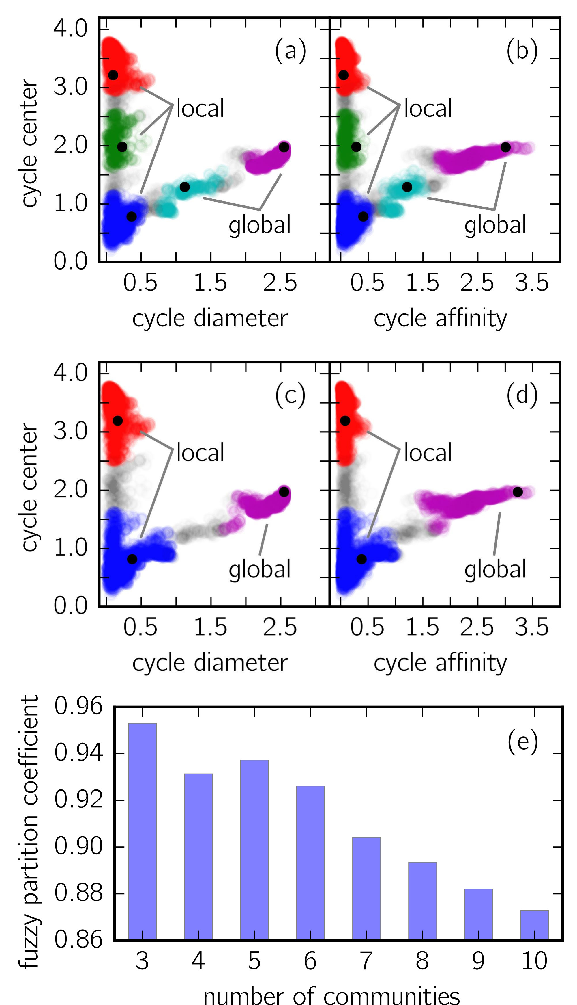
Figure 3: Cycle space ($\dot{\gamma}=1.6$). (a) Scatter plot of cycle center vs. the cycle diameter, and (b) cycle affinity vs. cycle center. The cycle diameter and centers are computed using a PCA (see text for details). Colors represent cycle communities while gray points indicate no community. The filled black circles indicate the cycle representatives. (c,d) The same plots as for (a,b) but for three cycle communities. (e) The fuzzy partition coefficients computed for multiple communities. The best result is obtained for 3 communities followed by a slightly lower value for 5 communities.

We can turn these insights into a more quantitative statement by partitioning the cycle space into $k$ communities. To this end we employ an implementation of the fuzzy $c$-means algorithm (an implementation is available in Ref. 33), which assigns to each cycle a probability for belonging to a specific community. First, we normalize all three features (cycle diameters, cycle centers, and affinities) by their variance to make them comparable. These features are then used as an input for the fuzzy c-means clustering algorithm returning membership degrees $u_{ij}$ which express the probability that observation $i$ belongs to community $j$. To obtain an indicator of how good the clustering results are we compute the fuzzy partition coefficient (FPC) that is defined as the Frobenius norm of the membership matrix

$$\text{FPC}=\frac{1}{n}\sum_{i=1}^{k}\sum_{j=1}^{n}u_{ij}^{2}.$$ (7)

Here $k$ is the number of chosen communities and $n$ the number of observations (cycles in our case). The closer the FPC gets to one the better the cycle space can be partitioned into the chosen number of clusters.

The advantage of fuzzy partitioning is that some cycles might not belong to any cycle community while others match well in multiple ones. The minimal number of cycle communities to account for the collective folding and unfolding dynamics is $k=3$ (see Fig. 3e), but to capture the full dynamics we found $k=5$ cycle communities to be more appropriate. We identify three local communities colored in blue, green, and red, as well as two global communities colored in magenta and cyan, see Fig. 3a,b. The blue community represents cycles that correspond to globular configurations while the green and red communities represent similar dynamics for intermediate and fully stretched configurations, respectively. The global cycle communities connect two (cyan) or all three (magenta) local communities.

III.3 Coarse-graining

Next, we replace each cycle community by one cycle that we will refer to as representative Knoch and Speck (2015). We find appropriate representatives by mapping mean first-passage times between states that belong to different local cycle communities. After selecting representatives, we delete all states not belonging to any of the representatives and rescale the remaining transition rates with restrictions that: the total entropy production rate $\dot{S}$, all remaining cycle affinities $A_{\alpha}$ and all remaining edge affinities $A^{i}_{j}$ are preserved. For details see Ref. 22 and appendix C.

At this stage the coarse-grained MSM still contains many states since a single cycle can traverse hundreds of states. The important point is, however, that the coarse-grained model lost much of its original complexity as it now contains only a few cycles. We can thus further reduce the number of states. To this end we identify two dominant motifs, which we refer to as bridge and triangle states. Both motifs build on states that have exactly two neighbors. For bridge states the neighbors are not connected to each other Altaner and Vollmer (2012). Triangle states complete cycles that do not exhibit positive entropy productions and thus are not part of the decomposition Eq. (4). We iteratively search and remove these states (for details see appendix D) until no more are found, which completes our coarse-graining scheme.

IV Coarse-grained NE-MSM

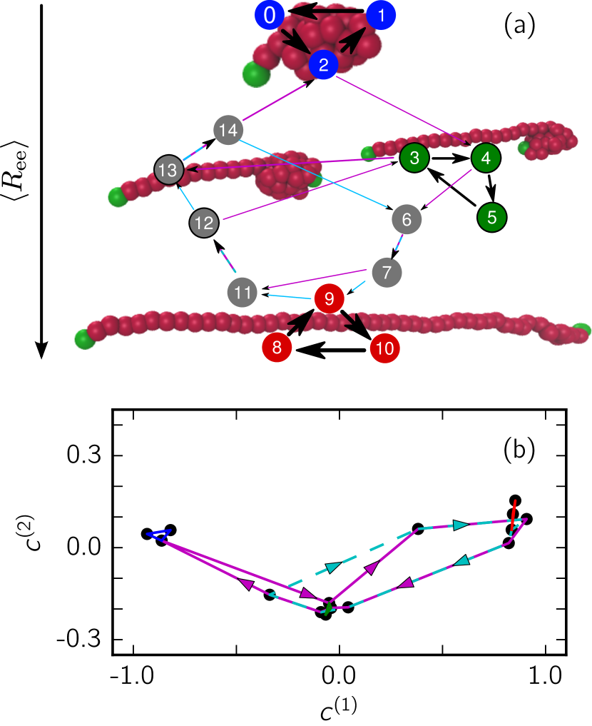
Figure 4: Final NE-MSM for $\dot{\gamma}=1.6$. (a) Transition network of the polymer dynamics with 15 centroids (filled circles) and 5 cycles. The colored states green, blue, and red correspond to the colors of the local cycle communities shown in Fig. 3. States with a black border are structurally very similar and constitute the transition ensemble. The arrows point in the direction of probability currents (net flux), while the arrow widths represent the magnitude of currents. On average, the polymer dynamics follows the direction of the arrows. Arrow colors cyan and magenta correspond to the global cycles. (b) Transition network in configuration space using the normalized projections onto the two largest principal components. Symbols are the configurations while lines indicate the cycles with the arrows pointing in the direction of the net flux.

The final NE-MSM for strain rate $\dot{\gamma}=1.6$ is shown in Fig. 4a. After removing the bridge and triangle states the transition network contains 15 states (centroids). The collective rates for folding and unfolding of this coarse-grained model agree with those obtained from the BD simulations by construction. Moreover, the remaining five cycles now allow for detailed insights into the relevant pathways in non-equilibrium. The three local cycles are composed of three states, the minimal number for a non-trivial, entropy-producing cycle. The red and blue cycle connect stable globular and stretched configurations, respectively. The green cycle represents a metastable intermediate of half-stretched configurations that do not unfold correctly but quickly fold back to the intermediate. The global cyan cycle also contains half-stretched configurations (structurally similar to the green cycle) but here the unfolding reaches the final stretched states before returning to their half-stretched origin. Finally, the magenta cycle represents the full transition from globule to stretched configurations and back.

The five states $(3,4,5,12,13)$ describing intermediate, half-stretched configurations are very close in configuration space (see Fig. 4b). They constitute the analog of the transition ensemble through which the folding/unfolding has to proceed. In non-equilibrium, however, the folding and unfolding processes follow different paths through this narrow region of configuration space. The globule to half-stretched transition proceeds along $2\to 4$ (with state 4 belonging to the green cycle) whereas the reverse half-stretched to globule transition proceeds along $13\to 14\to 2$, with states 13 and 14 belonging to the cyan cycle. The cycle topology thus reveals the dynamical trapping of the polymer in an intermediate, which cannot be captured by structural information alone. Employing order parameters like distances in configuration space or lifetimes to identify mesostates will clearly miss this important feature of cyclic non-equilibrium dynamics.

Another question that we can address is dissipation, the role of which for bio-processes has been investigated recently, e.g., for self-replication England (2013) and in the activation of signaling proteins Weber et al. (2015). The rate of dissipated heat $\dot{Q}_{\text{diss}}=\dot{S}/T$ created in each cycle community is proportional to their respective entropy production rate $\dot{S}$. Our analysis reveals that both the blue and red cycles are equally responsible for about 30% of the total dissipated heat, while the green, cyan, and magenta communities produce 5%, 15%, and 50%, respectively. The latter is caused by the large conformational changes (folding and unfolding process) of the polymer. The blue and red cycles, on the other hand, do not exhibit large conformational changes, therefore, the conformational changes must be on very short timescales, which is confirmed by the large probability currents shown in Fig. 4a.

We finally comment on using a PCA, which is not necessarily the best method to reduce the dimensionality of configuration space, and more advanced methods such as the time-lagged independent correlation analysis exist Pérez-Hernández et al. (2013). Moreover, it is common practice to first apply a dimensionality reduction to the continuous molecular dynamics (or BD) data and subsequently discretize the reduced configuration space into finite sets. We did not follow this approach because NE-MSMs built from reduced configuration space exhibit a significantly lower entropy production rate than NE-MSMs built from full configuration space (assuming the same number of centroids is used). Recent results Barato and Seifert (2015); Gingrich et al. (2016) suggest that the fluctuations of general currents are bounded by the entropy production, which directly links dynamic with thermodynamic consistency.

V Conclusions

To conclude, we have presented a general method to systematically construct coarse-grained models composed of a few discrete states from molecular data of steadily driven systems. Specifically, we have studied the globule-stretch transition of a simple model polymer, but the method can in principle be applied to more realistic and complex molecules (such as F₁-ATPase Sugawa et al. (2016)), delivering minimal and thermodynamically consistent Markov state models. While these models can be employed to bridge time scales, they also allow insights into the relevant transition pathways. Here we have shown that different directions can pass through the same region of configuration space, which we believe might be a general property of transitions in driven systems.

Appendix A Spatial clustering

The configuration space is discretized by employing the popular $k$-means clustering algorithm which divides the continuous configuration space into $k$ volumes and returns their centroids (center of each volume). Next the BD trajectories are projected onto the centroids, storing its dynamical information as simple sequences of centroid indices. We extract the dynamical information by counting the number of transitions $C_{i\to j}(\tau)$ for a given lag time $\tau$ (time in between transitions). The count matrix $\boldsymbol{C}(\tau)$ is used to approximate the transition matrix $\boldsymbol{T}(\tau)$ by

$$T_{i\to j}(\tau)=\frac{C_{i\to j}(\tau)}{\sum_{j}C_{i\to j}(\tau)},$$ (8)

which is also the maximum probability estimator for the true transition operator Prinz et al. (2011). We additionally require $\boldsymbol{T}$ to have two important properties: First, $\boldsymbol{T}$ must be ergodic, i.e. each state can be reached from every other state in finite time or the transition network spanned by $\boldsymbol{T}$ is connected. Second, all occurring transitions are reversible, i.e. if $T^{i}_{j}>0$ then $T^{j}_{i}>0$.

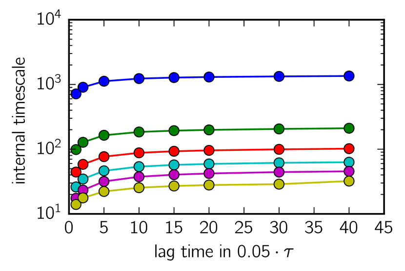
Figure 5: Lag time analysis. The six slowest internal timescales are plotted for different lag times. For building the MSM we choose $\tau=20$.

If the process described by $\boldsymbol{T}$ is time-homogeneous its entries $T^{i}_{j}$ are ought to be time-independent. To test this we perform a lag time analysis Swope et al. (2004) shown in Fig. 5. For equilibrium systems the eigenvalues $\lambda_{i}$ of the transition matrix $\boldsymbol{T}$ can be converted into relaxation timescales of the system $t_{i}=-\tau/\log{(\lambda_{i})}$ with slowest modes corresponding to the largest $\lambda_{i}$. If the largest eigenvalues are time-independent, also the slowest modes are time-independent yielding a good estimation of the minimal lag time that can be used. In NE-MSM the eigenvalues can become complex, which leaves their physical interpretation still open for discussion. However, for the polymer dynamics the largest eigenvalues sorted by either their real part or absolute value exhibit no imaginary part.

For a continuous-time Markov process with rate matrix $\boldsymbol{W}$, the transition probability can be expressed as $\boldsymbol{T}=e^{\boldsymbol{W}\tau}$. While conventional Markov state models have discrete-time dynamics, for our purposes we require a rate matrix, which we approximate from the computed transition matrix through

$$\boldsymbol{W}\approx\frac{\boldsymbol{T}-\mathbf{1}}{\tau}.$$ (9)

All off-diagonal elements of $\boldsymbol{W}$ are non-negative $\omega^{i}_{j}\geq 0$ while the diagonal elements are $\omega^{i}_{i}=-\sum_{j}\omega^{i}_{j}$. Following the Perron-Frobenius theorem, $\boldsymbol{T}$ and thus $\boldsymbol{W}$ have an unique largest real eigenvalue $\lambda_{\text{max}}$ with a corresponding eigenvector that has strictly positive entries. This eigenvector represents the steady-state probability distribution with elements $p_{i}$. Finally, the probability fluxes are obtained by $\Phi^{i}_{j}=\omega^{i}_{j}p_{i}$.

Appendix B Cycle decomposition

Here we describe an algorithm that decomposes a given probability flux matrix $\boldsymbol{\Phi}$ into cycle fluxes. Each element of $\boldsymbol{\Phi}$ transforms through $\Phi^{i}_{j}=\sum_{(i\to j)\ni\alpha}\varphi_{\alpha}$ with $\varphi_{\alpha}\geq 0$. The sum adds the cycle weights of all cycles containing the edge $i\to j$. For the cycle decomposition we start by dividing $\boldsymbol{\Phi}$ into a symmetric detailed-balance part $\boldsymbol{\Phi}^{\text{db}}$ and a non-negative current part $\boldsymbol{J}$ so that

$$\boldsymbol{\Phi}=\boldsymbol{\Phi}^{\text{db}}+\boldsymbol{J}.$$ (10)

Here $\boldsymbol{J}$ is obtained by $\boldsymbol{\Phi}-\boldsymbol{\Phi}^{T}$ with all negative elements set to zero. The symmetric part follows as $\boldsymbol{\Phi}^{\text{db}}=\boldsymbol{\Phi}-\boldsymbol{J}$. To make progress, we identify all non-zero elements of $\boldsymbol{\Phi}^{\text{db}}$ yielding a set of trivial cycles, i.e. cycles with only two different states ($i\to j\to i$). Their cycle weights are identical to their corresponding non-zero entry $\varphi_{i\to j\to i}\equiv\Phi^{i\,\text{db}}_{j}=\Phi^{j\,\text{db}}_{i}$. The algorithm to decompose the current part $\boldsymbol{J}$ is split into two parts. First, searching for a non-trivial cycles (cycle with more than 2 different states) and second determining its cycle weights. Theoretically, the number of possible non-trivial cycles grows exponentially with the number of non-zero entries of $\boldsymbol{J}$. However, if both steps run alternately the decomposition becomes computationally affordable even for a large number of states. To detect a non-trivial cycle, we propose the following steps:

1. Find the position of the largest element of $\boldsymbol{J}$, $\operatorname{arg\,max}(J^{i}_{j})$.

2. Search for the shortest path (smallest number of transitions) from state $j$ leading back to state $i$ (only following the non-zero transitions). This step can be efficiently achieved by applying a breadth-fist/depth-first search Newman (2010).

3. Return the non-trivial cycle, i.e. ($i\to j\to\,$found path).

To determine the corresponding cycle weight $\varphi_{\alpha}$, we take all flux values along cycle $\alpha$ and determine their smallest value becoming the cycle weight

$$\varphi_{\alpha}\equiv\min_{i\to j\in\alpha}\{J^{i}_{j}\}.$$ (11)

Summing up both steps, the final algorithm reads

1. Find a non-trivial cycle

2. Compute its cycle weight $\varphi_{\alpha}$

3. Update the current matrix by subtracting $\varphi_{\alpha}$ along $\alpha$, $\boldsymbol{J}=\boldsymbol{J}-\sum_{(i\to j)\in\alpha}\varphi_{\alpha}$ and repeat with the first step

4. The algorithm stops when the residuum $||\boldsymbol{J}_{\text{max}}||$ has become smaller than a threshold.

General considerations Kalpazidou (2007); Altaner et al. (2012) show that the maximum number of needed non-trivial cycles is bounded by $N_{\text{cycles}}=|E|-|V|+1$ with $|E|$ being the number of non-zero elements of $\boldsymbol{J}$ and $|V|$ its rank.

Appendix C Cycle representatives and coarse-graining

Once the cycle communities are found, the idea for coarse-graining the MSM is to pick one cycle for each community – we refer to it as representative –, delete all states not belonging to any representative and, finally, rescale the remaining transition rates $\omega^{i}_{j}$. To be thermodynamically consistent the newly computed transition rates have to preserve four quantities: The total entropy production rate $\dot{S}$, the cycle affinities of the representatives $A_{\alpha}$, all remaining edge affinities $A^{i}_{j}$ and the dissipated heat along the remaining edges $\log{(\omega^{i}_{j})}-\log{(\omega^{j}_{i})}$. For a detailed description of the coarse-graining algorithm we refer the reader to our previous publication Knoch and Speck (2015).

Since we know now how to coarse-grain a given set of cycle representatives, we address the question of how to select “appropriate” representatives. Any set of cycle representatives is thought to be appropriate if the graph spanned by their coarse-grained transition matrix is ergodic and the mean first passage times (MFPT) between local communities are preserved. For example, the polymer dynamics for $k=3$ communities as illustrated in Fig. 3c,d exhibits 2 local and 1 global community. To compute the MFPTs we identify all states of the red community, say as set $R$, and all states belonging to the blue one as set $B$. Any appropriate set of representatives needs to preserve MFPT_R→B and MFPT_B→R.

Especially, the conservation of MFPTs is of particular importance as it ensures the coarse-grained MSM to express the correct timescales. So far no determinstic algorithm exists that returns a reliable set of representatives. For this reason we formulate a stochastic algorithm that picks candidates for cycle representatives randomly and checks for ergodicity and MFPTs. The algorithm is outlined as follows:

1. Choose one representative per cycle community by drawing a random number.

2. Check if set of representatives span ergodic transition network. If yes, compute coarse-grained MSM, else go back to step (1).

3. Compute MFPTs of the coarse-grained MSM and compare to MFPTs of full MSM. If MFPTs match, return coarse-grained MSM, else go back to step (1).

Appendix D Coarse-graining of bridge and triangle states

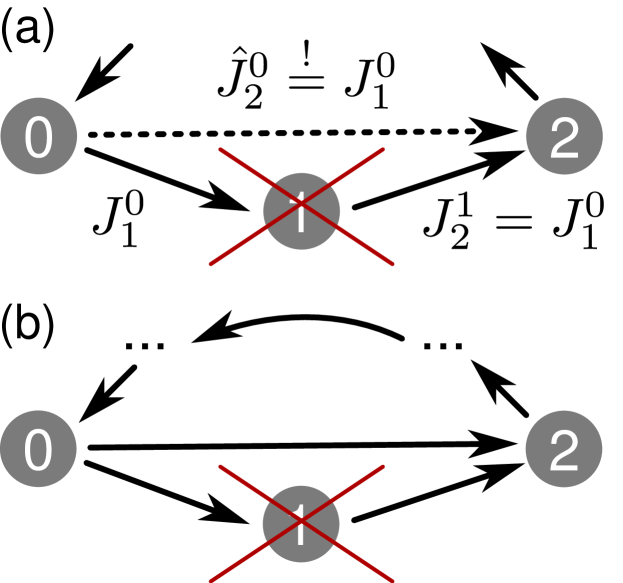
Figure 6: Illustration of bridge and triangle state coarse-graining approach. (a) Bridge state: After deletion of state 1 the other states are directly connected (dotted arrow). (b) Triangle state: After deletion of state 1 the existing connections $0\leftrightarrow 2$ are modified. The arrows point in the direction of probability currents.

To coarse-grain bridge states (state 1 in Fig. 6a) we form a new connection between the two neighboring states (state 0 and 2 in Fig. 6a). The new transition rates $\hat{\omega}^{0}_{2}$ and $\hat{\omega}^{2}_{0}$ have to preserve three characteristics: (i) edge affinities $\hat{A}^{0}_{2}=A^{0}_{1}+A^{1}_{2}$, (ii) probability currents $\hat{J}^{0}_{2}=J^{0}_{1}=J^{1}_{2}$ and (iii) dissipated heat $\log{(\hat{\omega}^{0}_{2}/\hat{\omega}^{2}_{0})}=\log{(\omega^{0}_{1}/\omega^{1}_{0})}+\log{(\omega^{1}_{2}/\omega^{2}_{1})}$. Using conditions (i) and (ii), the new probability fluxes follow as

$$\hat{\Phi}^{0}_{2} =\hat{\Phi}^{2}_{0}\frac{\Phi^{0}_{1}\Phi^{1}_{2}}{\Phi^{1}_{0}\Phi^{2}_{1}}~{}\text{ and }~{}\hat{\Phi}^{0}_{2}=\hat{\Phi}^{2}_{0}+\Phi^{0}_{1}-\Phi^{1}_{0}$$

$$\Rightarrow\hat{\Phi}^{2}_{0} =\frac{\Phi^{0}_{1}-\Phi^{1}_{0}}{\left(\frac{\Phi^{0}_{1}\Phi^{1}_{2}}{\Phi^{1}_{0}\Phi^{2}_{1}}\right)-1}$$ (12)

To fulfill condition (iii) we demand that the ratio between any two probabilities of the full network are preserved $\hat{p}_{i}/\hat{p}_{j}=p_{i}/p_{j}$, which includes $\hat{p}_{0}/\hat{p}_{2}=p_{0}/p_{2}$, and thus

$$\frac{w^{i}_{j}}{w^{j}_{i}}=\frac{\Phi^{i}_{j}}{\Phi^{j}_{i}}\frac{p_{j}}{p_{i}}=\frac{\hat{\Phi}^{i}_{j}}{\hat{\Phi}^{j}_{i}}\frac{\hat{p}_{j}}{\hat{p}_{i}}=\frac{\hat{w}^{i}_{j}}{\hat{w}^{j}_{i}}.$$ (13)

Condition (iii) is also the main difference between our approach and the one discussed in Ref. 34. In our adaptation the probability distribution of the complete network is changed, while Altaner et al. change it only locally ($p_{0}$ and $p_{2}$) and hence absorb $p_{1}$ into $p_{0}$ and $p_{2}$. The disadvantage of the latter is that condition (iii) is not preserved for the full network and, when using the coarse-graining approach iteratively, accumulation of probability in single states might occur, which leads to unphysical results.

For the coarse-graining of triangle states (state 1 in Fig. 6b) we consider all cycles that contain the edges $0\to 1\to 2$. We modify these cycles by replacing the edges $0\to 1\to 2$ with a new edge $0\to 2$. To be thermodynamically consistent the modified cycles have to (i) preserve the cycle entropy production rate $\dot{S}_{\alpha}\equiv\varphi_{\alpha}A_{\alpha}$, (ii) preserve the edge affinities $A^{0}_{2}$ and (iii) dissipated heat $\log{(\omega^{0}_{2}/\omega^{2}_{0})}$. To rescale the transition rates we use the same rescaling algorithm as for the rescaling of the cycle representatives. Note that through restriction (i) it is not necessarily possible to coarse-grain all found triangle structures. Assume, for instance, that the modified cycle coincides with an already existing cycle, then, the rescaling is not unique anymore and entropy production is destroyed as only one out of two cycles survives.

References

- Karplus and McCammon (2002) M. Karplus and J. A. McCammon, “Molecular dynamics simulations of biomolecules,” Nat. Struct. Mol. Biol. 9, 646–652 (2002).
- Kamerlin et al. (2011) S. C. L. Kamerlin, S. V. A. Dryga, and A. Warshel, “Coarse-grained (multiscale) simulations in studies of biophysical and chemical systems,” Ann. Rev. Phys. Chem. 62, 41–64 (2011).
- Müller-Plathe (2002) F. Müller-Plathe, “Coarse-graining in polymer simulation: From the atomistic to the mesoscopic scale and back,” ChemPhysChem 3, 754–769 (2002).
- Harmandaris and Kremer (2009) V. A. Harmandaris and K. Kremer, “Dynamics of polystyrene melts through hierarchical multiscale simulations,” Macromol. 42, 791–802 (2009).
- Salerno et al. (2016) K. M. Salerno, A. Agrawal, D. Perahia, and G. S. Grest, “Resolving dynamic properties of polymers through coarse-grained computational studies,” Phys. Rev. Lett. 116, 058302 (2016).
- Noé and Fischer (2008) F. Noé and S. Fischer, “Transition networks for modeling the kinetics of conformational change in macromolecules,” Curr. Opin. Struct. Biol. 18, 154–162 (2008).
- Noé et al. (2009) F. Noé, C. Schütte, E. Vanden-Eijnden, L. Reich, and T.R. Weikl, “Constructing the equilibrium ensemble of folding pathways from short off-equilibrium simulations,” Proc. Natl. Acad. Sci. USA 106, 19011–19016 (2009).
- Bowman et al. (2011) G. R. Bowman, V. A. Voelz, and V. S. Pande, “Taming the complexity of protein folding,” Curr. Opin. Struct. Biol. 21, 4 – 11 (2011).
- Prinz et al. (2011) J.-H. Prinz, H. Wu, M. Sarich, B. Keller, M. Senne, M. Held, J. D. Chodera, C. Schütte, and F. Noé, “Markov models of molecular kinetics: Generation and validation,” J. Chem. Phys. 134, 174105 (2011).
- Dobson (2003) C. M. Dobson, “Protein folding and misfolding,” Nature 426, 884–890 (2003).
- Noé (2015) F. Noé, “Beating the millisecond barrier in molecular dynamics simulations,” Biophys. J. 108, 228–229 (2015).
- Larson (2005) R. G. Larson, “The rheology of dilute solutions of flexible polymers: Progress and problems,” J. Rheol. 49, 1–70 (2005).
- Smith et al. (1999) D. E. Smith, H. P. Babcock, and S. Chu, “Single-polymer dynamics in steady shear flow,” Science 283, 1724–1727 (1999).
- De Gennes (1974) P. G. De Gennes, “Coil-stretch transition of dilute flexible polymers under ultrahigh velocity gradients,” J. Chem. Phys. 60, 5030–5042 (1974).
- Doyle et al. (2000) P. S. Doyle, B. Ladoux, and J.-L. Viovy, “Dynamics of a tethered polymer in shear flow,” Phys. Rev. Lett. 84, 4769–4772 (2000).
- Delgado-Buscalioni (2006) R. Delgado-Buscalioni, “Cyclic motion of a grafted polymer under shear flow,” Phys. Rev. Lett. 96, 088303 (2006).
- Zhang et al. (2009) Y. Zhang, A. Donev, T. Weisgraber, B. J. Alder, M. D. Graham, and J. J. de Pablo, “Tethered dna dynamics in shear flow,” The Journal of Chemical Physics 130, 234902 (2009).
- Wang and Schütte (2015) H. Wang and C. Schütte, “Building markov state models for periodically driven non-equilibrium systems,” J. Chem. Theory Comput. 11, 1819–1831 (2015).
- Koltai et al. (2016) P. Koltai, G. Ciccotti, and C. Schütte, On Markov state models for non-equilibrium molecular dynamics, Tech. Rep. 16-11 (ZIB, Takustr.7, 14195 Berlin, 2016).
- Pellegrini et al. (2016) F. Pellegrini, F. P. Landes, A. Laio, S. Prestipino, and E. Tosatti, “Markov state modeling of sliding friction,” arXiv:1605.03849 (2016).
- Puglisi et al. (2010) A. Puglisi, S. Pigolotti, L. Rondoni, and A. Vulpiani, “Entropy production and coarse graining in markov processes,” J. Stat. Mech. , P05015 (2010).
- Knoch and Speck (2015) F. Knoch and T. Speck, “Cycle representatives for the coarse-graining of systems driven into a non-equilibrium steady state,” New J. Phys. 17, 115004 (2015).
- Seifert (2012) U. Seifert, “Stochastic thermodynamics, fluctuation theorems, and molecular machines,” Rep. Prog. Phys. 75, 126001 (2012).
- Alexander-Katz et al. (2006) A. Alexander-Katz, M. F. Schneider, S. W. Schneider, A. Wixforth, and R. R. Netz, “Shear-flow-induced unfolding of polymeric globules,” Phys. Rev. Lett. 97, 138101 (2006).
- Winkler (2006) R. G. Winkler, “Semiflexible polymers in shear flow,” Phys. Rev. Lett. 97, 128301 (2006).
- Lemak et al. (1998) A. S. Lemak, N. K. Balabaev, Y. N. Karnet, and Y. G. Yanovsky, “The effect of a solid wall on polymer chain behavior under shear flow,” J. Chem. Phys. 108, 797–806 (1998).
- Altaner et al. (2012) B. Altaner, S. Grosskinsky, S. Herminghaus, L. Katthän, M. Timme, and J. Vollmer, “Network representations of nonequilibrium steady states: Cycle decompositions, symmetries, and dominant paths,” Phys. Rev. E 85, 041133 (2012).
- Kalpazidou (2007) S. L. Kalpazidou, Cycle representations of Markov processes, Vol. 28 (Springer Science & Business Media, 2007).
- Schnakenberg (1976) J. Schnakenberg, “Network theory of microscopic and macroscopic behavior of master equation systems,” Rev. Mod. Phys. 48, 571 (1976).
- Conrad et al. (2015) N. D. Conrad, R. Banisch, and C. Schütte, “Modularity of directed networks: Cycle decomposition approach,” J. Comput. Dyn. 2, 1–24 (2015).
- Note (1) The reason why the connectivity fails is presumably because the underlying potential energy landscape does not offer well separated basins.
- Jolliffe (2002) I. Jolliffe, Principal component analysis (Wiley Online Library, 2002).
- (33) http://pythonhosted.org/scikit-fuzzy.
- Altaner and Vollmer (2012) B. Altaner and J. Vollmer, “Fluctuation-preserving coarse graining for biochemical systems,” Phys. Rev. Lett. 108, 228101 (2012).
- England (2013) J. L. England, “Statistical physics of self-replication,” J. Chem. Phys. 139, 121923 (2013).
- Weber et al. (2015) J. K. Weber, D. Shukla, and V. S. Pande, “Heat dissipation guides activation in signaling proteins,” Proc. Natl. Acad. Sci. USA 112, 10377–10382 (2015).
- Pérez-Hernández et al. (2013) G. Pérez-Hernández, F. Paul, T. Giorgino, G. De Fabritiis, and F. Noé, “Identification of slow molecular order parameters for markov model construction,” J. Chem. Phys. 139, 015102 (2013).
- Barato and Seifert (2015) A. C. Barato and U. Seifert, “Thermodynamic uncertainty relation for biomolecular processes,” Phys. Rev. Lett. 114, 158101 (2015).
- Gingrich et al. (2016) T. R. Gingrich, J. M. Horowitz, N. Perunov, and J. L. England, “Dissipation bounds all steady-state current fluctuations,” Phys. Rev. Lett. 116, 120601 (2016).
- Sugawa et al. (2016) M. Sugawa, K. Okazaki, M. Kobayashi, T. Matsui, G. Hummer, T. Masaike, and T. Nishizaka, “F1-atpase conformational cycle from simultaneous single-molecule fret and rotation measurements,” Proc. Natl. Acad. Sci. USA 113, E2916–E2924 (2016).
- Swope et al. (2004) W. C. Swope, J. W. Pitera, and F. Suits, “Describing protein folding kinetics by molecular dynamics simulations. 1. theory,” J. Phys. Chem. B 108, 6571–6581 (2004).
- Newman (2010) M. Newman, Networks: An Introduction (Oxford university press, 2010).