Production of charmed baryons in $\bar{p}p$ collisions close to their thresholds

Abstract

Cross sections for the charm-production reactions $\bar{p}p\to\bar{\Lambda}_{c}^{-}\Sigma_{c}^{+}$, $\bar{\Sigma}_{c}\Sigma_{c}$, $\bar{\Xi}_{c}\Xi_{c}$, and $\bar{\Xi}_{c}^{\prime}\Xi_{c}^{\prime}$ are presented, for energies near their respective thresholds. The results are based on a calculation performed in the meson-exchange framework in close analogy to earlier studies of the Jülich group on the strangeness-production reactions $\bar{p}p\to\bar{\Lambda}\Sigma$, $\bar{\Sigma}\Sigma$, $\bar{\Xi}\Xi$ by connecting the two sectors via SU(4) flavor symmetry. The cross sections are found to be in the order of $0.1-1$ $\mu b$ at energies of $100$ MeV above the respective thresholds, for all considered channels. Complementary to meson-exchange, where the charmed baryons are produced by the exchange of $D$ and $D^{*}$ mesons, a charm-production potential derived in a quark model is employed for assessing uncertainties. The cross sections predicted within that picture turned out to be significantly smaller.

I Introduction

The FAIR project at the GSI laboratory has an extensive program aiming at a high-accuracy spectroscopy of charmed hadrons and at an investigation of their interactions with ordinary matter PANDA . For the feasibility of such studies, specifically those of the $\rm\bar{P}$ANDA experiment Wiedner:2011 the production rate for charmed hadrons in antiproton-proton (${\bar{p}p}$) is a key factor. Knowledge of such production rate is also relevant for studies of in-medium changes of charmed hadrons—for recent references, see Refs. in-medium1 ; in-medium2 ; Shyam:2016 . However, presently very little is known about the strength of the interaction of charmed hadrons with ordinary baryons and mesons. In view of that, over the last few years we have looked at the exclusive charm-production reactions ${\bar{p}p}\rightarrow\bar{\Lambda}_{c}^{-}{\Lambda}_{c}^{+}$ Haidenbauer:2010 and ${\bar{p}p}\rightarrow D\bar{D},\,D_{s}\bar{D}_{s}$ Haidenbauer:2014 ; Haidenbauer:2015 close to their thresholds with the objective to provide with our predictions estimations for the pertinent cross sections.

In the present paper we extend our study of the reaction ${\bar{p}p}\rightarrow\bar{\Lambda}_{c}^{-}{\Lambda}_{c}^{+}$ Haidenbauer:2010 to the production of other charmed baryons such as the $\Sigma_{c}$, the $\Xi_{c}$ and the $\Xi_{c}^{\prime}$. The projected antiproton beam-momentum available for the $\rm\bar{P}$ANDA experiment reaches up to $15$ GeV/c corresponding to a center-of-mass energy of $\sqrt{s}=5.5$ GeV Boca . Thus, the production of most of the charmed members of the lowest SU(4) $J^{P}=1/2^{+}$ baryon $20$-plet is possible at $\rm\bar{P}$ANDA, including the $\Xi_{c}$ and $\Xi_{c}^{\prime}$ and even the $\Omega_{c}^{0}$ PDG . While there is a large number of calculations for ${\bar{p}p}\rightarrow\bar{\Lambda}_{c}^{-}{\Lambda}_{c}^{+}$ Kroll:1988cd ; Kaidalov:1994mda ; Titov:2008 ; Goritschnig:2009sq ; Khodjamirian:2012 ; Shyam:2014 ; Wang:2016 this can not be said for the production of other charmed baryons. Khodjamirian et al. Khodjamirian:2012 published cross sections for $\bar{\Lambda}_{c}^{-}{\Sigma}_{c}^{+}$ and ${\bar{\Sigma}_{c}\Sigma_{c}}$. Titov and Kämpfer provided results for $d\sigma/dt$, for $\bar{\Lambda}_{c}^{-}{\Sigma}_{c}^{+}$ and ${\bar{\Sigma}_{c}\Sigma_{c}}$ in Titov:2008 and for ${\bar{\Xi}_{c}\Xi_{c}}$ in Titov:2011 . However, their analysis focusses on the region of small momentum transfer and integrated cross sections are not given. The earliest study we are aware of where integrated cross sections for ${\bar{\Sigma}_{c}^{--}\Sigma_{c}^{++}}$ were presented is the one by Kroll et al. Kroll:1988cd .

Our analysis of charm production is done in complete analogy to that of the reactions ${\bar{p}p}\rightarrow{\bar{\Lambda}\Lambda},{\bar{\Lambda}\Sigma},{\bar{\Sigma}\Sigma},{\bar{\Xi}\Xi}$ performed by the Jülich group some time ago Haidenbauer:1991 ; Haidenbauer:1992 ; Haidenbauer:1993 ; Haidenbauer:XX . In those studies the hyperon-production reaction is considered within a coupled-channel model. This allows to take into account rigorously the effects of the initial (${\bar{p}p}$) and final (${\bar{Y}Y}$) state interactions which play an important role for energies near the production threshold Haidenbauer:1991 ; Haidenbauer:1992 ; Kohno ; Alberg . The microscopic strangeness production is described by meson exchange and arises from the exchange of the $K$ and $K^{*}$ mesons. The elastic parts of the interactions in the initial (${\bar{p}p}$) and final (${\bar{Y}Y}$) states are likewise described by meson exchange, while annihilation processes are accounted for by phenomenological optical potentials. Specifically, the elastic parts of the initial- (ISI) and final-state interactions (FSI) are $G$-parity transforms of an one-boson-exchange variant of the Bonn $NN$ potential obepf and of the hyperon-nucleon model A of Ref. Holzenkamp89 , respectively. With this model a good overall description of the ${\bar{p}p}\to{\bar{\Lambda}\Lambda}$, ${\bar{p}p}\to{\bar{\Lambda}\Sigma}{\rm+c.c.}$, and ${\bar{p}p}\to{\bar{\Sigma}\Sigma}$ data obtained in the P185 experiment at LEAR (CERN) PS185 could be achieved and its results are also in line with the scarce experimental information for ${\bar{p}p}\to{\bar{\Xi}\Xi}$ Haidenbauer:XX .

The extension of the model to the charm sector is based on SU(4) flavor symmetry. Accordingly, the elementary charm production process is described by $t$-channel $D$ and $D^{*}$ meson exchanges. Note that the symmetry is invoked primarily as guideline for providing constraints on the pertinent baryon-meson coupling constants. Though we do not expect that the SU(4) symmetry should hold, recent calculations of the relevant coupling constants within QCD light-cone sum rules suggest that the actual deviation from the SU(4) values could be only in the order of a factor $2$ or even less Khodjamirian:2012 ; even smaller deviations have been obtained 3p0 in a constituent quark model calculation using the ${}^{3}P_{0}$ pair-creation mechanism. We examine the sensitivity of the results to variations in the elastic and annihilation parts of the initial ${\bar{p}p}$ interaction. Furthermore, as already done for $\bar{\Lambda}_{c}^{-}{\Lambda}_{c}^{+}$ Haidenbauer:2010 , we investigate the effect of replacing the meson-exchange transition by a charm-production potential derived in a quark model. Again this serves for assessing uncertainties in the model, since one could question the validity of a meson-exchange description of the transition in view of the large masses of the exchanged mesons. In this context we want to note that meson-exchange as well as the quark model lead to rather short ranged transition potentials. Thus, practically speaking those can be viewed as being contact interactions where the pertinent coupling constants are simply saturated Epelbaum:2001 by the dynamics underlying the two considered approaches.

In the next two Sections we introduce the basic ingredients of the model. In Section IV we present numerical results for total cross sections for the various ${\bar{Y}_{c}Y_{c}}$ channels, utilizing for the charm-production mechanism meson-exchange as well as the quark model. A summary of our work is presented in Section V. Details on the transition potential in the quark model and on the SU(4) coupling constants that enter the meson-exchange transition potential are collected in Appendices.

II The model

We calculate the charm production reactions ${\bar{p}p}\rightarrow\bar{Y}_{c}Y_{c}$ in close analogy to the original Jülich coupled channel approach Haidenbauer:1991 ; Haidenbauer:1992 ; Haidenbauer:1993 ; Haidenbauer:XX to strangeness production. The transition amplitude is obtained from the solution of a multi-channel Lippmann-Schwinger (LS) equation,

$$\bm{T} = \bm{V}+\bm{V\,G_{0}\,T},$$ (1)

which reads explicitly in terms of the channels $\mu$ ($\nu$) corresponding to ${\bar{N}N}$, $\bar{\Lambda}_{c}^{-}{\Lambda}_{c}^{+}$, $\bar{\Lambda}_{c}^{-}{\Sigma}_{c}^{+}$, $\bar{\Sigma}_{c}^{-}{\Lambda}_{c}^{+}$, ${\bar{\Sigma}_{c}\Sigma_{c}}$, and ${\bar{\Xi}_{c}\Xi_{c}}$,

$$T^{\mu\nu}(\mathbf{p}_{\mu},\mathbf{p}_{\nu},z) = V^{\mu\nu}(\mathbf{p}_{\mu},\mathbf{p}_{\nu},z)+\sum_{\gamma}\int d^{3}p_{\gamma}\,V^{\mu\gamma}(\mathbf{p}_{\mu},\mathbf{p}_{\gamma},z)\,G_{0}^{\gamma}(\mathbf{p}_{\gamma},z)\,T^{\gamma\nu}(\mathbf{p}_{\gamma},\mathbf{p}_{\nu},z),$$ (2)

Here $z$ is the total energy and $\mathbf{p}_{\nu}$ ($\mathbf{p}_{\mu}$) the relative momentum in the initial (final) state in the center-of-mass. The propagator, $G_{0}(\mathbf{p},z)$, is given by

$$G_{0}^{\gamma}(\mathbf{p}_{\gamma},z)=1/(z-E^{\gamma}_{\mathbf{p}_{\gamma}}+i\epsilon)$$ (3)

with $E^{1}_{\mathbf{p}_{1}}=E^{\bar{N}}_{\mathbf{p}_{{\bar{N}N}}}+E^{N}_{\mathbf{p}_{{\bar{N}N}}}$, etc., being the relativistic energies of the two baryons in the intermediate state. The calculations are performed in isospin basis, which is sufficient for an exploratory study. Moreover, the mass splitting between $\Sigma^{++}_{c}$, $\Sigma^{+}_{c}$, and $\Sigma^{0}_{c}$ is rather small PDG . This is different in the strangeness sector where there is a sizable mass difference between the $\Sigma^{+}$, $\Sigma^{0}$, and $\Sigma^{-}$ which made a calculation in the particle basis mandatory Haidenbauer:1993 .

The transition potential from ${\bar{N}N}$ to the ${\bar{Y}_{c}Y_{c}}$ channel is given by $t$-channel $D$ and $D^{*}$ exchanges, see Fig. 1 (upper row). The expressions for the transition potentials are the same as for $K$ and $K^{*}$ exchange and can be found in Ref. Holzenkamp89 . They are of the generic form

$$V^{{\bar{Y}_{c}Y_{c}},{\bar{N}N}}(t)\sim\sum_{M=D,D^{*}}g_{\bar{N}\bar{Y}_{c}M}g_{NY_{c}M}\frac{F_{\bar{N}\bar{Y}_{c}M}(t)F_{NY_{c}M}(t)}{t-m^{2}_{M}},$$ (4)

where $g_{NY_{c}M}$ are coupling constants and $F_{NY_{c}M}(t)$ are form factors. Under the assumption of $SU(4)$ symmetry the coupling constants are identical to those in the corresponding strangeness production reaction for ${\bar{N}N}\to\bar{\Lambda}_{c}^{-}{\Lambda}_{c}^{+}$, ${\bar{N}N}\to\bar{\Lambda}_{c}^{-}{\Sigma}_{c}^{+},\bar{\Sigma}_{c}^{-}{\Lambda}_{c}^{+}$, and ${\bar{N}N}\to{\bar{\Sigma}_{c}\Sigma_{c}}$, but differ for ${\bar{\Xi}_{c}\Xi_{c}}$, see Appendix B. With regard to the vertex form factors we use here a monopole form with a cutoff mass $\Lambda$ of 3 GeV, at the $NY_{c}D$ as well as at the $NY_{c}D^{*}$ vertex, as in our study of $\bar{\Lambda}_{c}^{-}{\Lambda}_{c}^{+}$ production Haidenbauer:2010 .

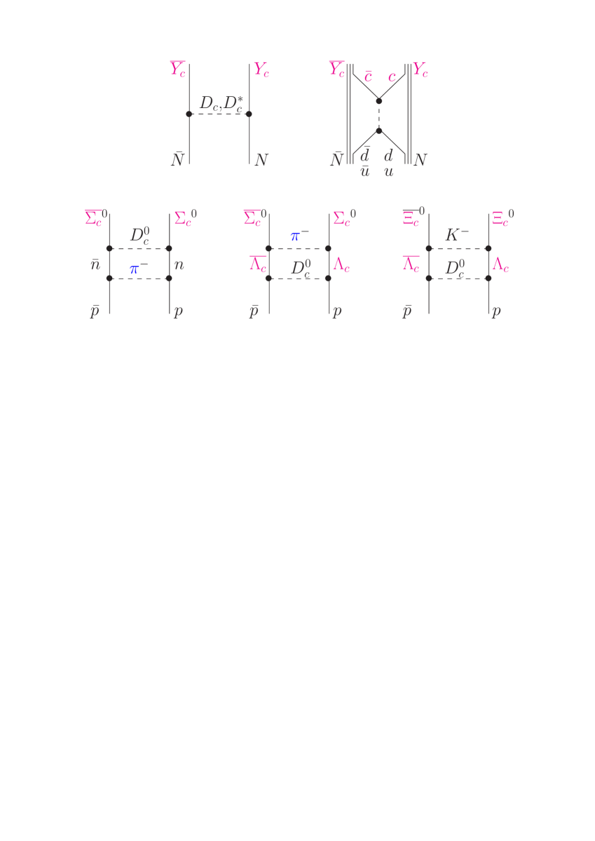
Figure 1: Upper row: Contributions to the $\bar{N}N\to\bar{Y}_{c}Y_{c}$ transition potential $V^{\mu\nu}$ in the meson-exchange picture (left) and the quark model (right). Lower row: Selected contributions to the ${\bar{p}p}\to\bar{\Sigma}_{c}^{0}\Sigma_{c}^{0}$ and ${\bar{p}p}\to\bar{\Xi}_{c}^{0}\Xi_{c}^{0}$ transition amplitude generated by the coupled channel framework.

The ${\bar{\Xi}_{c}\Xi_{c}}$ channel cannot be reached from ${\bar{N}N}$ via single meson exchange, and the same is also the case for $\bar{\Sigma}_{c}^{0}\Sigma_{c}^{0}$ from an initial ${\bar{p}p}$ state. The corresponding transition potentials $V^{\mu\nu}$ are zero. However, the employed coupled-channel framework, cf. Eq. (2), generates automatically multistep processes so that the corresponding transition amplitudes $T^{\mu\nu}$ are no longer zero. Some contributions that arise at the first iteration in the LS equation are depicted in the lower row of Fig. 1. In principle, there are also contributions from non-iterative two-meson exchanges. However, we expect those to be much less important in comparison to iterated one-meson exchange. In the latter case the two baryons in the intermediate states can go on-shell and the pertinent contributions are accordingly enhanced Weinberg .

The diagonal potentials $V^{\mu\mu}$ are given by the sum of an elastic part and an annihilation part. For the ${\bar{N}N}$ channel we use again the set of potentials introduced and described in Refs. Haidenbauer:2010 ; Haidenbauer:2014 . Their elastic part is loosely connected (via G-parity transform) to a simple, energy-independent one-boson-exchange $NN$ potential (OBEPF). However, since at the high energies necessary for charm production any $NN$ potential has to be considered as being purely phenomenological several variants were constructed in order to explore how strongly the results on charm production depend on the choice of the ${\bar{N}N}$ interaction. In two of those variants (called A and A’ in Haidenbauer:2010 ; Haidenbauer:2014 ) only the longest ranged (and model-independent) part of the elastic ${\bar{N}N}$ interaction, namely one-pion exchange, was kept. Model B and C include also some short-range contributions, see the discussion in Haidenbauer:2010 .

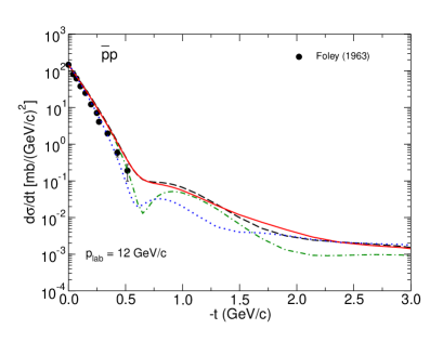
Figure 2: Differential cross section for elastic ${\bar{p}p}$ scattering at $p_{lab}$ = 12 GeV/c as a function of $t$. The curves represent results based on the ${\bar{N}N}$ potentials A (dash-dotted line), A’ (dotted), B (dashed) and C (solid), see text for details. The experimental information is taken from Foley et al. Foley .

All variants are supplemented by a phenomenological spin-, isospin-, and energy-independent optical potential of Gaussian form, in order to take into account annihilation,

$$V^{{\bar{N}N}\to{\bar{N}N}}_{opt}(r)=(U_{0}+iW_{0})\,e^{-r^{2}/2r^{2}_{0}}.$$ (5)

The free parameters ($U_{0}$, $W_{0}$, $r_{0}$) were determined by a fit to ${\bar{N}N}$ data in the energy region relevant for the reactions ${\bar{p}p}\to\bar{\Lambda}_{c}^{-}{\Lambda}_{c}^{+}$ and ${\bar{p}p}\to D\bar{D}$, i.e. for laboratory momenta of $p_{lab}=6-10$ GeV/c. (Their actual values can be found in Table 1 of Ref. Haidenbauer:2010 .) The data set comprises total cross sections, and integrated elastic and charge-exchange (${\bar{p}p}\to\bar{n}n$) cross sections. With all four variants a rather satisfying description of the ${\bar{N}N}$ data in that energy region could be obtained as documented in Refs. Haidenbauer:2010 ; Haidenbauer:2014 . Even at $p_{lab}=12$ GeV/c, i.e. at a momentum that corresponds roughly to the ${\bar{\Xi}_{c}\Xi_{c}}$ threshold, the differential cross section is nicely reproduced by all models, as exemplified in Fig. 2. Evidently, not only the magnitude at very forward angles but also the slope is reproduced well by all considered ${\bar{N}N}$ interactions. We want to emphasize that differential cross sections were not included in the fitting procedure and are, therefore, predictions of the models.

Note that yet another ${\bar{N}N}$ model was considered in Haidenbauer:2010 , namely Model D, which is based on the full G-parity transformed OBEPF. However, its results disagree considerably with the empirical ${\bar{p}p}$ differential cross sections as well as with the integrated charge-exchange cross sections and, thus, cannot be considered to be realistic. Because of that it was no longer utilized in our study of ${\bar{p}p}\to D\bar{D}$ Haidenbauer:2014 ; Haidenbauer:2015 and we will not use it here either.

In Ref. Haidenbauer:2010 the interaction in the final $\bar{\Lambda}_{c}^{-}{\Lambda}_{c}^{+}$ system was assumed to be the same as the one in ${\bar{\Lambda}\Lambda}$. Specifically, this means that the elastic part of the interaction is fixed by coupling constants and vertex form factors taken from the hyperon-nucleon model A of Ref. Holzenkamp89 , while the annihilation part is again parameterized by an optical potential which contains, however, spin-orbit and tensor components in addition to a central component Haidenbauer:1991 :

$$V^{\bar{\Lambda}_{c}^{-}{\Lambda}_{c}^{+}\to\bar{\Lambda}_{c}^{-}{\Lambda}_{c}^{+}}_{opt}(r) = \bigl{[}U_{c}+iW_{c}+(U_{LS}+iW_{LS})\,\mathbf{L}\cdot\mathbf{S}$$ (6)

$$+\,(U_{t}+iW_{t})\,\bm{\sigma}_{\Lambda_{c}}\cdot\mathbf{r}\,\bm{\sigma}_{\bar{\Lambda}_{c}}\cdot\mathbf{r}\bigr{]}\,e^{-r^{2}/2r^{2}_{0}}.$$

The free parameters in the optical ${\bar{\Lambda}\Lambda}$ potential were determined in Ref. Haidenbauer:1991 by a fit to data on total and differential cross sections, and analyzing power for ${\bar{p}p}\to{\bar{\Lambda}\Lambda}$. As already emphasized in Haidenbauer:2010 , we do not expect that the $\bar{\Lambda}_{c}^{-}{\Lambda}_{c}^{+}$ interaction will be the same on a quantitative level. But at least the bulk properties should be similar, because in both cases near threshold the interactions will be govered by strong annihilation processes. In the present study we need also interactions in the final $\bar{\Lambda}_{c}^{-}{\Sigma}_{c}^{+}$, ${\bar{\Sigma}_{c}\Sigma_{c}}$, and ${\bar{\Xi}_{c}\Xi_{c}}$ systems. Those interactions have been fixed by adopting the same philosophy as for $\bar{\Lambda}_{c}^{-}{\Lambda}_{c}^{+}$ and the parameters are likewise taken over from corresponding studies in the strangeness sector Haidenbauer:1993 ; Haidenbauer:XX .

III Transition potential from the constituent quark model

As an alternative to meson exchange we consider a charm-production potential inspired by quark-gluon dynamics. The strange-hadron production in $p\bar{p}$ reactions has been studied extensively within the constituent quark model in the past. The best known works are perhaps those of Kohno and Weise Kohno , Furui and Faessler Furui , Burkardt and Dillig Burkardt , Roberts Roberts and Alberg, Henley and Wilets Alberg . For an extensive list of references see the review PS185 and for a fairly recent work Ref. Ortega:2012 . In the present study we adopt the interaction proposed by Kohno and Weise, derived in the so-called ${}^{3}S_{1}$ mechanism. In this model the $\bar{s}s$ (or $\bar{c}c$) pair in the final state is created from an initial $\bar{u}u$ or $\bar{d}d$ pair via $s$-channel gluon exchange, see Fig. 1. After quark degrees-of-freedom are integrated out the potential has the form Kohno :

$${V}^{{\bar{p}p}\to{\bar{\Lambda}\Lambda}}(r)=\frac{4}{3}A_{1}(\alpha,\beta)^{3/2}\frac{4\pi\tilde{\alpha}}{m_{G}^{2}}\delta_{S1}\left(\frac{3}{4\pi\langle{r}^{2}\rangle}\right)^{3/2}\exp\left[-\frac{3}{4}B_{1}(\alpha,\beta)\frac{r^{2}}{\langle{r}^{2}\rangle}\right]\ ,$$ (7)

$${V}^{{\bar{p}p}\to\bar{\Lambda}\Sigma^{0},\bar{\Sigma}^{0}\Lambda}(r)=-\frac{4}{3\sqrt{3}}A_{1}(\alpha,\beta)^{3/2}\frac{4\pi\tilde{\alpha}}{m_{G}^{2}}(\delta_{S0}+\frac{2}{3}\delta_{S1})\,\left(\frac{3}{4\pi\langle{r}^{2}\rangle}\right)^{3/2}\exp\left[-\frac{3}{4}B_{1}(\alpha,\beta)\frac{r^{2}}{\langle{r}^{2}\rangle}\right]\ ,$$ (8)

$${V}^{{\bar{p}p}\to{\bar{\Sigma}^{0}\Sigma^{0}}}(r)=\frac{8}{27}A_{1}(\alpha,\beta)^{3/2}\frac{4\pi\tilde{\alpha}}{m_{G}^{2}}(\delta_{S0}+\frac{21}{18}\delta_{S1})\,\left(\frac{3}{4\pi\langle{r}^{2}\rangle}\right)^{3/2}\exp\left[-\frac{3}{4}B_{1}(\alpha,\beta)\frac{r^{2}}{\langle{r}^{2}\rangle}\right]\ ,$$ (9)

$${V}^{{\bar{p}p}\to{\bar{\Sigma}^{-}\Sigma^{+}}}(r)=2\,{V}^{{\bar{p}p}\to{\bar{\Sigma}^{0}\Sigma^{0}}}(r),\quad\quad{V}^{{\bar{p}p}\to{\bar{\Sigma}^{+}\Sigma^{-}}}(r)=0\ .$$ (10)

The corresponding expressions for the transitions to charmed baryons (${{\bar{p}p}\to\bar{\Lambda}_{c}^{-}{\Lambda}_{c}^{+}}$, etc.) are formally identical. The quantity ${\tilde{\alpha}}/{m_{G}^{2}}$ in Eqs. (7)-(9) is an effective (quark-gluon) coupling strength, $\langle{r}^{2}\rangle$ is the mean square radius associated with the quark distribution in the nucleon and $S$ is the total spin in the ${\bar{p}p}$ system. The effective coupling strength is practically a free parameter that was fixed by a fit to the ${\bar{p}p}\to{\bar{\Lambda}\Lambda}$ data Haidenbauer:1992 . Contrary to Ref. Kohno and to our initial study Haidenbauer:2010 now we take into account the quark-mass dependence of the intrinsic wave functions of the baryons. This dependence is encoded in the functions $A_{1}(\alpha,\beta)$ and $B_{1}(\alpha,\beta)$ for which explicit expressions can be found in Appendix A, together with the transition potentials to other channels such as ${\bar{\Xi}\Xi}$. For equal quark masses $A_{1}$ and $B_{1}$ reduce to $1$ so that one recovers the result of Kohno and Weise. However, considering the difference in the constituent quark masses of the strange and the charmed quark one arrives at somewhat different strengths and ranges for the transition potentials in the strangeness and charm sectors. Choosing $\langle{r}^{2}\rangle^{1/2}=0.571$ fm and ${\tilde{\alpha}}/{m_{G}^{2}}=0.252$ fm² ensures agreement with the parameters used in our studies of ${\bar{p}p}\to{\bar{\Lambda}\Lambda}$ Haidenbauer:1992 and ${\bar{p}p}\to{\bar{\Lambda}\Sigma}$ Haidenbauer:1993 .

The effective coupling strength depends explicitly on the effective gluon propagator $m_{G}^{2}$, i.e. on the square of the energy transfer from initial to final quark pair, cf. Refs. Furui ; Burkardt ; Kohno1 . Heuristically this energy transfer corresponds roughly to the masses of the produced constituent quarks, i.e. $m_{G}\approx 2m_{q}$ so that we expect the effective coupling strength ${\tilde{\alpha}}/{m_{G}^{2}}$ for charm production to be reduced by the ratio of the constituent quark masses of the strange and the charmed quark squared, $(m_{s}/m_{c})^{2}\approx$ (550 MeV / 1600 MeV)² $\approx$ 1/9 as compared to the one for ${\bar{p}p}\to{\bar{\Lambda}\Lambda}$. This reduction factor is adopted in our calculation for the charm sector.

In the calculation for the quark-model transition potential the same diagonal interactions (${\bar{N}N}\to{\bar{N}N}$, ${\bar{\Lambda}\Lambda}\to{\bar{\Lambda}\Lambda}$, …) as described in the last section are employed. However, the parameters in the optical potentials for ${\bar{\Lambda}\Lambda}$ (cf. Eq. (6)) have been re-adjusted in order to ensure a reproduction of the ${\bar{p}p}\to{\bar{\Lambda}\Lambda}$ data Haidenbauer:1992 and the same has been done in Ref. Haidenbauer:1993 for ${\bar{\Lambda}\Sigma}$+c.c. and now for the new data on the ${\bar{\Sigma}\Sigma}$ channels. For the extension to the charm sector we assume again that the ${\bar{Y}_{c}Y_{c}}$ interactions are the same as those for ${\bar{Y}Y}$.

IV Results

Before we present our results for charm production let us discuss briefly the reaction ${\bar{p}p}\to{\bar{\Sigma}\Sigma}$. When the Jülich group published their results back in 1993 Haidenbauer:1993 the only experimental information on the ${\bar{\Sigma}\Sigma}$ channel at low energies consisted in a preliminary data point for ${\bar{\Sigma}^{-}\Sigma^{+}}$. In the meantime the final result for ${\bar{\Sigma}^{-}\Sigma^{+}}$ has become available Barnes:1997 and also a measurement for ${\bar{\Sigma}^{+}\Sigma^{-}}$ Johansson:1999 . The latter channel is of particular interest because it requires a double charge-exchange and, therefore, at least a two-step process. In our model calculation such processes are generated automatically by solving the LS equation (2), and it had been predicted in Ref. Haidenbauer:1993 that ${\bar{\Sigma}^{+}\Sigma^{-}}$ production is by no means suppressed at low energies as one could have expected. The actual measurement of the cross section, published several years after our calculation Johansson:1999 , nicely confirmed this prediction, see Fig. 3 (left). Results for ${\bar{p}p}\to{\bar{\Sigma}\Sigma}$ based on the constituent quark-model had not been presented in Ref. Haidenbauer:1993 . This is done here for the first time, see Fig. 3 (right). Information on the model results for ${\bar{p}p}\to{\bar{\Lambda}\Lambda}$ and ${\bar{p}p}\to{\bar{\Lambda}\Sigma}$ can be readily found in Refs. Haidenbauer:1991 ; Haidenbauer:1992 ; Haidenbauer:1993 (for the meson-exchange and the quark-model) and we refrain from reproducing those here.

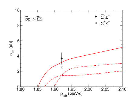
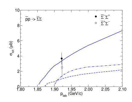
Figure 3: Cross sections for ${\bar{p}p}\to\Sigma\bar{\Sigma}$. On the left results based on the meson-exchange transition potential are displayed while on the right those for the quark model are shown. The solid, dashed, and dash-dotted lines correspond to ${\bar{\Sigma}^{-}\Sigma^{+}}$, ${\bar{\Sigma}^{0}\Sigma^{0}}$, and ${\bar{\Sigma}^{+}\Sigma^{-}}$, respectively. Data taken at $p_{lab}=1.922$ GeV/c are from Refs. Barnes:1997 ; Johansson:1999 . The symbols are placed at slightly lower and higher momenta, respectively, so that the error bars do not overlap.

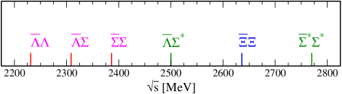
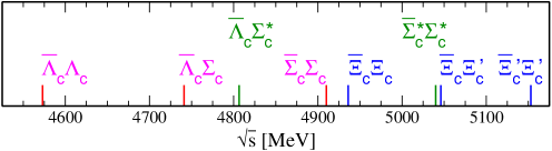
Figure 4: Thresholds of various channels in the strangeness and charm sectors. $\Sigma^{*}$ stands for the $\Sigma^{*}$(1385) and $\Sigma_{c}^{*}$ for the $\Sigma_{c}^{*}$(2520) $3/2^{+}$ resonances. Thresholds involving $1/2^{-}$ baryons such as the $\Lambda$(1405), for example, are not displayed.

It is instructive to recall the kinematical situation for the production of strange and charmed baryons in ${\bar{p}p}$ collisions. This is done in Fig. 4 where the thresholds of the various channels are indicated. One can see that the openings of the ${\bar{\Lambda}\Lambda}$, ${\bar{\Lambda}\Sigma}$, and ${\bar{\Sigma}\Sigma}$ channels are much closer together than those of their charmed counterparts. On the other hand, the ${\bar{\Xi}\Xi}$ threshold is much farther away than that of ${\bar{\Xi}_{c}\Xi_{c}}$. And in the charmed case there are in addition thresholds involving the $\Xi_{c}^{\prime}$. We indicate also the thresholds of channels that involve the $3/2^{+}$ baryons $\Sigma^{*}$(1385) and $\Sigma_{c}^{*}$(2520). Those channels are not included in the present study which aims at a rough and qualitative estimation of the (strangeness and) charm production cross section. It should be said, however, that their presence could have a sizable quantitative impact on the production cross sections, specifically in those reactions whose thresholds lie above the ones for the production of $3/2^{+}$ baryons.

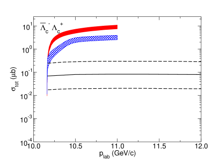
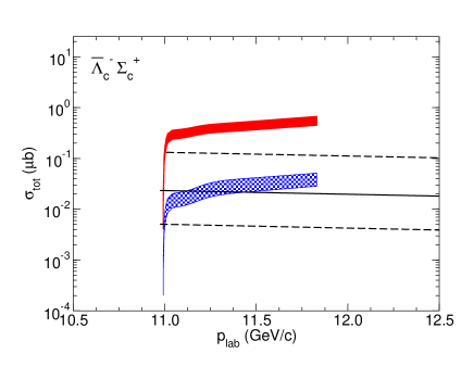
Figure 5: Cross sections for ${\bar{p}p}\to\bar{\Lambda}_{c}^{-}{\Lambda}_{c}^{+}$ (left) and ${\bar{p}p}\to\bar{\Lambda}_{c}^{-}{\Sigma}_{c}^{+}$ (right) as a function of $p_{lab}$. The solid (red) bands are results based on the meson-exchange transition potential, the hatched (blue) bands are for the quark model. The solid and dashed lines are results taken from Ref. Khodjamirian:2012 , see text.

Predictions for the charm production reactions ${\bar{p}p}\to\bar{\Lambda}_{c}^{-}{\Lambda}_{c}^{+}$ and ${\bar{p}p}\to\bar{\Lambda}_{c}^{-}{\Sigma}_{c}^{+}$ are shown in Fig. 5. The meson-exchange result for ${\bar{p}p}\to\bar{\Lambda}_{c}^{-}{\Lambda}_{c}^{+}$ is identical to the one presented in Ref. Haidenbauer:2010 . However, as already said in Sec. III we no longer consider the unrealistic ${\bar{N}N}$ model D because it predicts a too large ${\bar{p}p}$ cross section and, as a consequence, leads to a much stronger reduction of the ${\bar{p}p}\to\bar{\Lambda}_{c}^{-}{\Lambda}_{c}^{+}$ amplitude as compared to the other ${\bar{N}N}$ potentials (A-C) that reproduce the ${\bar{N}N}$ data in the relevant energy region very well Haidenbauer:2010 ; Haidenbauer:2014 . Accordingly, the variation of the predicted production cross section due to differences in the employed ${\bar{N}N}$ ISI, represented by bands in Fig. 5, is now much smaller, namely less than a factor 2. Thus, for ${\bar{N}N}$ potentials that not only reproduce the integrated cross sections but also describe the ${\bar{p}p}$ differential cross in forward direction satisfactorily the resulting uncertainty in the predicted charm production cross sections remains modest. Evidently, now the bands from the meson-exchange and quark-model transition potentials are clearly separated. Note that for the latter in the present work the dependence of the mean square radius $\langle r^{2}\rangle$ on the quark masses is taken into account, cf. Sec. III, and because of that the predictions are slightly increased as compared to the ones shown in Ref. Haidenbauer:2010 .

Table 1: Production cross sections for strange and charmed baryons at the excess energy $\varepsilon$ = 25 MeV in $\mu b$. The corresponding laboratory momenta are indicated in the table. The variations in the charm case are those due to the $\bar{N}N$ models A-C. Note that the results for $\Xi_{c}^{\prime}\bar{\Xi}_{c}^{\prime}$ are from a truncated coupled-channel calculation, see text.

	Strangeness			Charm
	$p_{lab}$	Meson	Quark	$p_{lab}$	Meson	Quark
	(GeV/c)	exchange	model	(GeV/c)	exchange	model
${\bar{p}p}\to{\bar{\Lambda}\Lambda}$ ($\bar{\Lambda}_{c}^{-}{\Lambda}_{c}^{+}$)	1.507	24.7	27.7	10.28	2.65-4.00	0.66-1.27
${\bar{p}p}\to{\bar{\Lambda}\Sigma}$ ($\bar{\Lambda}_{c}^{-}{\Sigma}_{c}^{+}$)	1.724	5.84	6.38	11.12	0.32-0.49	0.01-0.02
${\bar{p}p}\to{\bar{\Sigma}^{-}\Sigma^{+}}$ (${\bar{\Sigma}_{c}^{--}\Sigma_{c}^{++}}$)	1.942	3.51	3.67	11.98	0.63-1.09	0.001
${\bar{p}p}\to{\bar{\Sigma}^{0}\Sigma^{0}}$ (${\bar{\Sigma}_{c}^{-}\Sigma_{c}^{+}}$)	1.942	1.40	1.45	11.98	0.19-0.29	0.001
${\bar{p}p}\to{\bar{\Sigma}^{+}\Sigma^{-}}$ (${\bar{\Sigma}_{c}^{0}\Sigma_{c}^{0}}$)	1.942	2.65	2.86	11.98	0.26-0.40	0.001
${\bar{p}p}\to{\bar{\Xi}^{0}\Xi^{0}}$ (${\bar{\Xi}_{c}^{-}\Xi_{c}^{+}}$)	2.677	0.21	0.45	12.15	0.42-0.60	0.003-0.005
${\bar{p}p}\to{\bar{\Xi}^{+}\Xi^{-}}$ (${\bar{\Xi}_{c}^{0}\Xi_{c}^{0}}$)	2.677	0.17	0.32	12.15	0.17-0.26	0.003-0.005
${\bar{p}p}\to{\bar{\Xi}_{c}^{\prime-}\Xi_{c}^{\prime+}}$				13.32	0.15-0.22	(0.5-0.7)$\cdot 10^{-4}$
${\bar{p}p}\to{\bar{\Xi}_{c}^{\prime 0}\Xi_{c}^{\prime 0}}$				13.32	0.05-0.08	(0.5-0.7)$\cdot 10^{-4}$

In order to facilitate a quantitative comparison between the two model approaches, but also between the predictions for charm production with those for the strangeness sector, we provide tables with results corresponding to the excess energies of $25$ MeV (Table 1) and $100$ MeV (Table 2) in the respective channels. One can see from those tables that the quark model yields ${\bar{p}p}\to\bar{\Lambda}_{c}^{-}{\Lambda}_{c}^{+}$ cross sections that are roughly a factor $2-3$ smaller than the ones based on meson exchange.

The ${\bar{p}p}\to\bar{\Lambda}_{c}^{-}{\Sigma}_{c}^{+}$ ($\bar{\Sigma}_{c}^{-}\Lambda_{c}^{+}$) cross sections predicted by the meson-exchange model are more or less an order of magnitude smaller than those for ${\bar{p}p}\to\bar{\Lambda}_{c}^{-}{\Lambda}_{c}^{+}$, cf. Fig. 5 and Tables 1 and 2. This could be somehow expected based on the corresponding ratio in the strangeness sector. On the other hand, the predictions based on the quark model are much smaller. In particular, they are roughly a factor $100$ smaller than the pertinent results for the $\bar{\Lambda}_{c}^{-}{\Lambda}_{c}^{+}$ channel, and they are a factor $30$ smaller than the $\bar{\Lambda}_{c}^{-}{\Lambda}_{c}^{+}$ results in the meson-exchange picture.

For the ease of comparison we include in Fig. 5 also results from Khodjamirian et al. Khodjamirian:2012 (solid curve; the dashed curves indicate the uncertainty.) In that study, following Kaidalov and Volkovitsky Kaidalov:1994mda , a non-perturbative quark-gluon string model is used where, however, now baryon-meson coupling constants from QCD lightcome sum rules are employed. Interestingly, those results obtained in a rather different framework are more or less in line with our quark-model predictions.

Results for the ${\bar{p}p}\to{\bar{\Sigma}_{c}\Sigma_{c}}$ channels are presented in Fig. 6. The cross sections predicted by the meson-exchange model are all of similar magnitude, even the one for ${\bar{\Sigma}_{c}^{0}\Sigma_{c}^{0}}$ where a two-step process is required. The magnitude is also comparable to the cross section for ${\bar{p}p}\to\bar{\Lambda}_{c}^{-}{\Sigma}_{c}^{+}$. Also here the results based on the quark model are significantly smaller, i.e. even by roughly three orders of magnitude. Again we include here the results from Khodjamirian et al. Khodjamirian:2012 . In this case only isospin averages results are available. Let us mention that Kroll et al. Kroll:1988cd have already published integrated cross sections for ${\bar{\Sigma}_{c}^{--}\Sigma_{c}^{++}}$ more than two decades ago. Their predictions amount to about $10^{-3}$ $\mu b$ at $p_{lab}=16$ GeV/c and, thus, are more or less compatible with those by Khodjamirian et al.

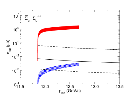
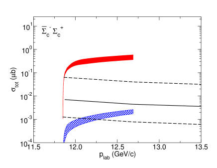
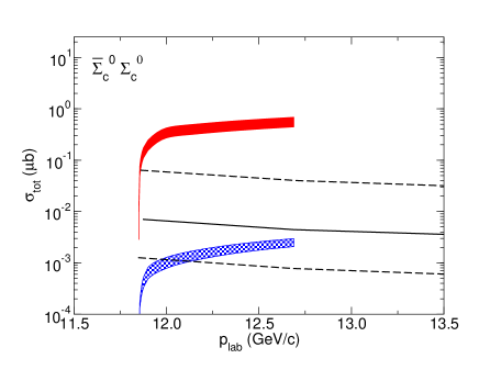
Figure 6: Cross sections for ${\bar{p}p}\to{\bar{\Sigma}_{c}\Sigma_{c}}$ as a function of $p_{lab}$. Top left: ${\bar{\Sigma}_{c}^{--}\Sigma_{c}^{++}}$, top right ${\bar{\Sigma}_{c}^{-}\Sigma_{c}^{+}}$, bottom: ${\bar{\Sigma}_{c}^{0}\Sigma_{c}^{0}}$.
Same description of curves as in Fig. 5.

Production cross sections for ${\bar{p}p}\to\Xi_{c}\bar{\Xi}_{c}$ are displayed in Fig. 7. The results exhibit a similar pattern to what we already observed for the ${\bar{\Sigma}_{c}\Sigma_{c}}$ case. Once again the cross sections based on the meson-exchange transition potential are in the order of $0.1-1$ $\mu b$ while the predictions for the quark model are orders of magnitude smaller. We performed also exploratory calculations for the reaction ${\bar{p}p}\to\Xi_{c}^{\prime}\bar{\Xi}_{c}^{\prime}$. Its threshold lies significantly higher than those of the other charmed baryons and several more channels are already open, see Fig. 4. Therefore, in this case only a very rough estimate can be expected from our model study. Because of that we omitted the $\Xi_{c}\bar{\Xi}_{c}$ and $\Xi_{c}\bar{\Xi}_{c}^{\prime},\,\Xi_{c}^{\prime}\bar{\Xi}_{c}$ channels in that calculation for simplicity reasons. The corresponding results are quoted in Tables 1 and 2.

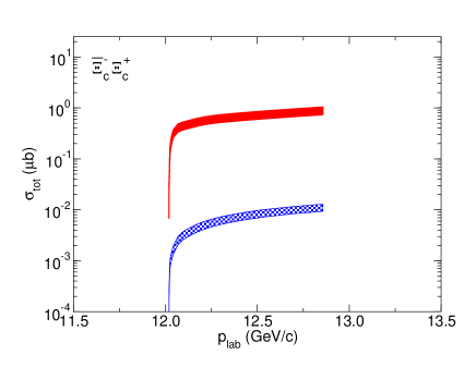
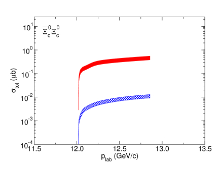
Figure 7: Cross sections for $\Xi_{c}\bar{\Xi}_{c}$ as a function of $p_{lab}$. Left: ${\bar{\Xi}_{c}^{-}\Xi_{c}^{+}}$, right ${\bar{\Xi}_{c}^{0}\Xi_{c}^{0}}$. Same description of curves as in Fig. 5.

There is a clear trend that the cross sections in the quark model become more and more suppressed as compared to those from meson-exchange for channels with higher lying thresholds. The main reason for the stronger suppression is presumably related to the exponential $r$ dependence of the potential, see the expressions in Sec. III and Appendix A. It amounts to $V^{\mu\nu}(q)\propto{\rm exp}(-q^{2}\langle r^{2}\rangle/3)$ in momentum space with $\mathbf{q}=\mathbf{p}_{\mu}-\mathbf{p}_{\nu}$ being the transferred momentum. With increasing masses of the baryons there is an increasing momentum mismatch between the on-shell momenta in the initial (${\bar{N}N}$) and final states and, because of the exponential $q^{2}$ dependence, the on-shell matrix elements are strongly reduced for transitions to higher channels. In the meson-exchange picture the potential is given by $V^{\mu\nu}(q)\propto 1/(-q^{2}-m^{2}_{M})$, see Eq. (4). Since $m_{M}$ is already of the order of $2$ GeV variations in $q^{2}$ due to the different charm thresholds have only a moderate effect on the strength of the (on-shell) potential.

In addition also the interactions in the final ${\bar{Y}_{c}Y_{c}}$ states play a more important role. For $\bar{\Lambda}_{c}^{-}{\Lambda}_{c}^{+}$ production we had found that the results are rather insensitive to the FSI Haidenbauer:2010 , leading to a reduction of the cross section in the order of only 10-15 % when it is switched off altogether. This is no longer the case for channels with higher lying thresholds. Indeed, an increased sensitivity is not too surprising in view of the fact that some channels like ${\bar{\Sigma}_{c}^{0}\Sigma_{c}^{0}}$ and, of course, ${\bar{\Xi}_{c}\Xi_{c}}$ can only be reached by two-step processes, which means via ${\bar{Y}_{c}Y_{c}}$ FSI effects. We explored the sensitivity by (arbitrarily) increasing the annihilation in the ${\bar{\Sigma}_{c}\Sigma_{c}}$ channel by multiplying the strength parameters of the ${\bar{\Sigma}_{c}\Sigma_{c}}$ annihilation potential with a factor 2 and found that this reduces the pertinent charm production cross sections by one order of magnitude. Note that specifically for the quark model, where the on-shell transition matrix elements are rather small as discussed above, off-shell rescattering in the various transitions becomes very important.

Table 2: Production cross sections for strange and charmed baryons at the excess energy $\varepsilon$ = 100 MeV in $\mu b$. The corresponding laboratory momenta are indicated in the table. The variations in the charm case are those due to the $\bar{N}N$ models A-C. Note that the results for $\Xi_{c}^{\prime}\bar{\Xi}_{c}^{\prime}$ are from a truncated coupled-channel calculation, see text.

	Strangeness			Charm
	$p_{lab}$	Meson	Quark	$p_{lab}$	Meson	Quark
	(GeV/c)	exchange	model	(GeV/c)	exchange	model
${\bar{p}p}\to{\bar{\Lambda}\Lambda}$ ($\bar{\Lambda}_{c}^{-}{\Lambda}_{c}^{+}$)	1.719	72.6	70.6	10.66	5.65-8.37	2.22-3.49
${\bar{p}p}\to{\bar{\Lambda}\Sigma}$ ($\bar{\Lambda}_{c}^{-}{\Sigma}_{c}^{+}$)	1.937	10.6	9.5	11.50	0.60-0.91	0.02-0.04
${\bar{p}p}\to{\bar{\Sigma}^{-}\Sigma^{+}}$ (${\bar{\Sigma}_{c}^{--}\Sigma_{c}^{++}}$)	2.157	5.63	8.48	12.38	0.91-1.58	0.002
${\bar{p}p}\to{\bar{\Sigma}^{0}\Sigma^{0}}$ (${\bar{\Sigma}_{c}^{-}\Sigma_{c}^{+}}$)	2.157	2.35	2.77	12.38	0.30-0.46	0.002
${\bar{p}p}\to{\bar{\Sigma}^{+}\Sigma^{-}}$ (${\bar{\Sigma}_{c}^{0}\Sigma_{c}^{0}}$)	2.157	3.27	3.66	12.38	0.38-0.58	0.002
${\bar{p}p}\to{\bar{\Xi}^{0}\Xi^{0}}$ (${\bar{\Xi}_{c}^{-}\Xi_{c}^{+}}$)	2.904	0.40	0.94	12.55	0.62-0.87	0.007-0.010
${\bar{p}p}\to{\bar{\Xi}^{+}\Xi^{-}}$ (${\bar{\Xi}_{c}^{0}\Xi_{c}^{0}}$)	2.904	0.29	0.76	12.55	0.31-0.45	0.007-0.010
${\bar{p}p}\to{\bar{\Xi}_{c}^{\prime-}\Xi_{c}^{\prime+}}$				13.74	0.27-0.39	(0.1-0.2)$\cdot 10^{-3}$
${\bar{p}p}\to{\bar{\Xi}_{c}^{\prime 0}\Xi_{c}^{\prime 0}}$				13.74	0.08-0.13	(0.1-0.2)$\cdot 10^{-3}$

The charm production cross sections based on the meson-exchange picture depend also sensitively on the form-factor parameters at the $NY_{c}D$ and $NY_{c}D^{*}$ vertices. As said in Sec. II, for the results discussed above a cutoff mass of $\Lambda=$ 3 GeV has been used. When reducing this value to 2.5 GeV the cross sections for ${\bar{p}p}\to\bar{\Lambda}_{c}^{-}{\Lambda}_{c}^{+}$ drop by roughly a factor 3 Haidenbauer:2010 . For the other charm production channels considered in the present paper such a decrease of the cutoff mass in the transition potential yields a reduction of a factor $5$ in the cross sections. One can view that variation as a further uncertainty of the predictions based on the meson-exchange model. If so one can conclude that the results of the meson-exchange and quark transition potentials for ${\bar{p}p}\to\bar{\Lambda}_{c}^{-}{\Lambda}_{c}^{+}$ are indeed compatible with each other. However, this is definitely not the case for the other charm production channels considered. In principle, employing even smaller cutoff masses would further decrease the cross sections of the meson-exchange charm-production mechanism. However, as argued in Ref. Haidenbauer:2010 , in view of the fact that the exchanged mesons have a mass of around 1.9 to 2 GeV we consider values below 2.5 GeV as being not really realistic.

Finally, a comment on the SU(4) flavor symmetry which is used here as guideline for providing constraints on the pertinent baryon-meson coupling constants. As already said in the Introduction, recent calculations of the relevant ($D$ and $D^{*}$) coupling constants within QCD light-cone sum rules suggest that the actual deviation from the SU(4) predictions could be in the order of a factor $2$ or smaller, see Table 1 in Ref. Khodjamirian:2012 . Indeed, in several cases the ratio of the $NY_{c}M$ to $NYM$ coupling constants turned out to be practically consistent with SU(4) symmetry (where that ratio is $1$) within the quoted uncertainty. In any case, since the coupling constants enter quadratically into the potential, see Eq. (4), and with the 4th power into the cross sections it follows that a factor $2$ ($1.5$) in the coupling constant implies roughly a variation in the order of a factor $16$ ($5$) in the cross section. Such variations are larger than those from the ${\bar{p}p}$ ISI represented by the bands. However, they are well within the difference we observe between the predictions based on the meson-exchange transition potential and those of the quark model.

V Summary

In this paper we presented predictions for the charm-production reaction ${\bar{p}p}\to\bar{\Lambda}_{c}^{-}{\Lambda}_{c}^{+}$, $\bar{\Lambda}_{c}^{-}{\Sigma}_{c}^{+}$, ${\bar{\Sigma}_{c}\Sigma_{c}}$, and ${\bar{\Xi}_{c}\Xi_{c}}$. The production process is described within the meson-exchange picture in close analogy to our earlier studies on ${\bar{p}p}\to{\bar{\Lambda}\Lambda}$ Haidenbauer:1991 , ${\bar{\Lambda}\Sigma}$, ${\bar{\Sigma}\Sigma}$ Haidenbauer:1993 , and ${\bar{\Xi}\Xi}$ Haidenbauer:XX by connecting the dynamics via SU(4) symmetry. The calculations were performed within a coupled-channels framework so that the interaction in the initial ${\bar{p}p}$ interaction, which plays a crucial role for reliable predictions, can be taken into account rigorously. The interactions in the various ${\bar{Y}_{c}Y_{c}}$ channels and the transitions between those channels are also included.

The obtained $\bar{\Lambda}_{c}^{-}{\Sigma}_{c}^{+}$ ($\bar{\Sigma}_{c}^{-}{\Lambda}_{c}^{+}$) production cross sections are in the order of $0.5-1$ $\mu b$ for energies not too far from the threshold. Thus, they are about a factor $10$ smaller than the corresponding cross sections for $\bar{\Lambda}_{c}^{-}{\Lambda}_{c}^{+}$. The ${\bar{\Sigma}_{c}\Sigma_{c}}$ cross sections are likewise in the order of $0.5-1$ $\mu b$ where those for ${\bar{\Sigma}_{c}^{--}\Sigma_{c}^{++}}$ are predicted to be somewhat larger than those for ${\bar{\Sigma}_{c}^{-}\Sigma_{c}^{+}}$ and ${\bar{\Sigma}_{c}^{0}\Sigma_{c}^{0}}$. The cross sections for ${\bar{\Xi}_{c}\Xi_{c}}$ production, for which the threshold is only slightly higher than the one for ${\bar{\Sigma}_{c}\Sigma_{c}}$, are found to be around $0.5$ $\mu b$.

In order to shed light on the model dependence of our results we investigated the effect of replacing the meson-exchange transition potential by a charm-production mechanism derived in a quark model. In our earlier work on the reaction ${\bar{p}p}\to\bar{\Lambda}_{c}^{-}{\Lambda}_{c}^{+}$ we had found that both pictures lead to predictions of essentially the same order of magnitude Haidenbauer:2010 . Thus, it seemed that the details of the production mechanism do not matter, only the involved scales and these are fixed by the masses of the exchanged mesons or, correspondingly, the constituent masses of the produced charmed quarks. Now, it turned out that our conclusion drawn from that work was perhaps too optimistic. The extension of the study to other charmed baryons in the present work revealed drastic differences between the predictions of the two production mechanisms for channels with higher thresholds. Specifically, for ${\bar{p}p}\to\bar{\Lambda}_{c}^{-}{\Sigma}_{c}^{+}$ $(\bar{\Sigma}_{c}^{-}{\Lambda}_{c}^{+})$ the quark model yields results that are more than one order of magnitude smaller than those obtained for the meson-exchange model and in case of ${\bar{p}p}\to{\bar{\Sigma}_{c}\Sigma_{c}}$ or ${\bar{p}p}\to{\bar{\Xi}_{c}\Xi_{c}}$ the differences even amount to three orders of magnitude.

Clearly, this large difference or uncertainty in our predictions is a bit disillusioning. But to some extent it does not really come unexpected. While for the lowest channel, $\bar{\Lambda}_{c}^{-}{\Lambda}_{c}^{+}$, the magnitude of the cross section is mostly influenced by the initial ${\bar{p}p}$ interaction (which is known and fixed from experimental data) this is no longer the case for the other reactions. Here two-step processes of the form ${\bar{p}p}\to\bar{\Lambda}_{c}^{-}{\Lambda}_{c}^{+}\to{\bar{\Sigma}_{c}\Sigma_{c}}$, ${\bar{p}p}\to\bar{\Lambda}_{c}^{-}{\Sigma}_{c}^{+}\,(\bar{\Sigma}_{c}^{-}{\Lambda}_{c}^{+})\to{\bar{\Sigma}_{c}\Sigma_{c}}$, etc. become increasingly important. Accordingly, the influence of the interactions in the $\bar{\Lambda}_{c}^{-}{\Lambda}_{c}^{+}$, $\bar{\Lambda}_{c}^{-}{\Sigma}_{c}^{+}$, …, channels become more significant and those are not constrained by any empirical information. Specifically, for the quark-model results these interactions play a decisive role because direct transitions are suppressed due to the large momentum mismatch. Accepting the difference between the predictions based on meson exchange and those for the quark model as the basic uncertainty of our model calculation leaves ample room and, thus, is not so uncouraging for pertinent measurements. The results for meson exchange taken alone convey a much more optimistic perspective for experimental efforts. In any case, which of those scenarios is closer to reality can be only decided by performing concrete experiments that will hopefully be pursued at FAIR in the future.

Acknowledgments We thank Ulf-G. Meißner for his careful reading of our manuscript and Albrecht Gillitzer for stimulating discussions. Work partially supported by Conselho Nacional de Desenvolvimento Científico e Tecnológico - CNPq, Grant No. 305894/2009-9 (GK), and Fundação de Amparo à Pesquisa do Estado de São Paulo - FAPESP, Grant No. 2013/01907-0 (GK).

Appendix A Quark model

The microscopic quark-model interaction of the strange- and charm-baryon production potentials is inspired by an $s-$channel one-gluon exchange amplitude for light quark-antiquark $\bar{l}l$ pair annihilation and heavy quark-antiquark $\bar{h}h$ pair creation that can be parametrized in terms of an effective quark-gluon coupling strength $\tilde{\alpha}/m^{2}_{G}$ as:

$$V(\bar{l}l\rightarrow\bar{h}h)=-\frac{4\pi\tilde{\alpha}_{s}}{m^{2}_{G}}\,C\,\mathbf{S}^{2}\,\delta^{3}(\mathbf{r}_{l}-\mathbf{r}_{\bar{l}})\,\delta^{3}(\mathbf{r}_{h}-\mathbf{r}_{\bar{h}})\,\delta^{3}(\mathbf{r}_{h}-\mathbf{r}_{l}),$$ (11)

where $C$ is the color matrix

$$C(\bar{l}l\rightarrow\bar{h}h) = \frac{1}{6}\sum^{8}_{a=1}\left[\left(\frac{\lambda^{a}}{2}\right)_{\bar{l}l}-\left(\frac{\lambda^{a}}{2}\right)^{*}_{\bar{h}h}\right]^{2},$$ (12)

and $\mathbf{S}$ is the total spin of the light quark-antiquark pair (or of the heavy antiquark-quark pair, any quark mass factors involved in either case are absorbed in the effective coupling). Also, $l$ stands for $(u,d)$ and, depending on the case, $h$ for $s$ or $c$. For example, while in the process $\bar{p}p\rightarrow\bar{\Lambda}\Lambda\,(\bar{\Lambda}_{c}\Lambda_{c})$, $h=s\,(c)$, in $\bar{\Lambda}\Lambda\rightarrow\bar{\Xi}_{c}\Xi_{c}$, $l=(u,d)$ and $h=c$, and so on.

To evaluate the transition potential, we need quark-model wave functions for the baryons and antibaryons. For simplicity, we use harmonic oscillator wave functions, that for the ground states are given by

$$\phi_{B}(\mathbf{r}_{1},\mathbf{r}_{2},\mathbf{r}_{2})=\phi_{B}(\bm{\rho},\bm{\lambda})=\left(\frac{1}{\pi b^{2}_{\rho}}\right)^{3/4}\left(\frac{1}{\pi b^{2}_{\lambda}}\right)^{3/4}\,\exp\left(-\frac{1}{2b^{2}_{\rho}}\bm{\rho}^{2}-\frac{1}{2b^{2}_{\lambda}}\bm{\lambda}^{2}\right),$$ (13)

where $\bm{\rho}$ and $\bm{\lambda}$ are the Jacobi coordinates $\bm{\rho}=\mathbf{r}_{1}-\mathbf{r}_{2}$ and $\bm{\lambda}=\mathbf{r}_{3}-(m_{1}\mathbf{r}_{1}+m_{2}\mathbf{r}_{2})/(m_{1}+m_{2})$, with $m_{1}$, $m_{2}$ and $m_{3}$ being the quarks masses. For example, for the proton we have $m_{1}=m_{2}=m_{u}$ and $m_{3}=m_{d}$ (in the present paper, we take $m_{u}=m_{d}\equiv m$), $b^{p}_{\rho}=\sqrt{2\,\langle r^{2}\rangle}$, and $b^{p}_{\lambda}=\sqrt{3/2\,\langle r^{2}\rangle}$, where $\langle r^{2}\rangle$ is the proton mean square radius. For $\Lambda$ ($\Sigma$), $m_{1}=m_{2}=m$, $m_{3}=m_{s}$, and the size parameters $b^{\Lambda}_{\rho}$ and $b^{\Lambda}_{\lambda}$ are related to those of the proton as $b^{\Lambda}_{\rho}=b^{p}_{\rho}$ and $b^{\Lambda}_{\lambda}=\sqrt{\alpha}\,b^{p}_{\lambda}$ (and analogous for $\Sigma$), where $\alpha$ depends on the quark masses as

$$\alpha^{2}=\frac{m_{s}+2m}{3m_{s}}.$$ (14)

For $\Lambda_{c}$ ($\Sigma_{c}$), $m_{s}$ in Eq. (14) is to be replaced by the charmed quark mass $m_{c}$. For $\Xi$ one has $m_{1}=m_{2}=m_{s}$ and $m_{3}=m$ and, analogous to $\Lambda$, one can relate the respective size parameters to those of the proton as $b^{\Xi}_{\rho}=b^{p}_{\rho}$ and $b^{\Xi}_{\lambda}=\sqrt{\beta}\,b^{p}_{\lambda}$, with

$$\beta^{2}=\frac{m+2m_{s}}{3m}.$$ (15)

Finally, for the $\Xi_{c}$ and $\Xi^{\prime}_{c}$ states, which involve $u(d)$, $s$ and $c$ quarks, in order to keep the calculation simple we define an average mass $\bar{m}=(m+m_{s})/2$ so that in the wave function (13) the size parameters are related to those of the proton as $b^{\Xi_{c}}_{\rho}=b^{p}_{\rho}$ and $b^{\Xi_{c}}_{\lambda}=\sqrt{\bar{\beta}}\,b^{p}_{\lambda}$, with

$${\bar{\beta}}^{2}=\frac{m_{c}+2\bar{m}}{3m_{c}}.$$ (16)

Given the microscopic interaction and the baryon and antibaryon wave functions, one can evaluate rather easily the transition potentials. For the transitions $\bar{p}p\rightarrow\bar{\Lambda}\Lambda,\bar{\Sigma}^{0}\Sigma^{0},\bar{\Lambda}\Sigma^{0},\bar{\Sigma}^{-}\Sigma^{+}$ the potentials have been given explicitly in Eqs. (7)-(10), where the functions $A_{1}(\alpha,\beta)$ and $B_{1}(\alpha,\beta)$ take into account the different sizes of the baryons due to quark-mass differences encoded in the parameters $\alpha$ and $\beta$ defined above:

$$A_{1}(\alpha,\beta)=\frac{2}{1+\alpha},\hskip 28.45274ptB_{1}(\alpha,\beta)=\frac{1+\alpha}{2\alpha}.\hskip 28.45274pt$$ (17)

The expressions for the corresponding charm-production potentials $\bar{p}p\rightarrow\bar{\Lambda}^{-}_{c}\Lambda^{+}_{c}$, …, are identical. But $\alpha$ and $\beta$ differ and, accordingly, the values of the factors $A_{1}$ and $B_{1}$. And, of course, also the effective coupling constant is different. The transition potentials for double-strange baryon production, $\bar{\Lambda}\Lambda,\bar{\Sigma}^{0}\Sigma^{0},\bar{\Lambda}\Sigma^{0},\bar{\Sigma}^{-}\Sigma^{0}\rightarrow\bar{\Xi}^{0}\Xi^{0},\bar{\Xi}^{+}\Xi^{-}$, can be written generically as

$$V^{\text{2-s\,prod}}(r)=A_{2}(\alpha,\beta)^{3/2}\left(\frac{4\pi\tilde{\alpha}}{m^{2}_{G}}\right)\left(\chi_{0}\,\delta_{S0}+\chi_{1}\,\delta_{S1}\right)\left(\frac{3}{4\pi\langle r^{2}\rangle}\right)^{3/2}\exp\left[-\frac{3}{4}B_{2}(\alpha,\beta)\frac{r^{2}}{\langle r^{2}\rangle}\right],$$ (18)

where

$$A_{2}(\alpha,\beta) = \frac{2^{9}\,\alpha^{4}\,\beta}{\left[3+5\beta+\alpha\left(5+3\beta\right)\right]\,\left[3+5\beta+6\alpha^{2}\left(-1+\beta\right)+12\alpha^{3}\beta+\alpha^{4}\left(3+9\beta\right)\right]},$$ (19)

$$B_{2}(\alpha,\beta) = \frac{2\,\alpha^{3}\,\left[3+5\beta+\alpha\left(5+3\beta\right)\right]}{3+5\beta+6\alpha^{2}\left(-1+\beta\right)+12\alpha^{3}\beta+\alpha^{4}\left(3+9\beta\right)}.$$ (20)

and $\chi_{0}$ and $\chi_{1}$ are color-spin-flavor coefficients whose values are given in Table 3 (we use the phase conventions of Ref. Close for the spin-flavor wave functions).

Table 3: Color-spin-flavor factors $\chi_{0}$ and $\chi_{1}$ for the transitions to double-strange baryons $\bar{\Xi}^{(0,+)}\Xi^{(0,-)}$.

Initial state$\;\;\;\rightarrow$	$\bar{\Lambda}\Lambda$	$\bar{\Sigma}^{0}\Sigma^{0}$	$\bar{\Lambda}\Sigma^{0}$	$\bar{\Sigma}^{-}\Sigma^{+}$	Final State  $\downarrow$
S=0	$\frac{8}{9}$	-$\frac{16}{27}$	$\frac{4}{9\sqrt{3}}$	-$\frac{32}{27}$	$\bar{\Xi}^{0}\;\Xi^{0}$
	$\frac{8}{9}$	-$\frac{16}{27}$	-$\frac{4}{9\sqrt{3}}$	$0$	$\bar{\Xi}^{+}\Xi^{-}$
S=1	$\frac{28}{27}$	$\frac{52}{81}$	$\frac{16}{9\sqrt{3}}$	$\frac{104}{27}$	$\bar{\Xi}^{0}\;\Xi^{0}$
	$\frac{28}{27}$	$\frac{52}{81}$	-$\frac{16}{9\sqrt{3}}$	$0$	$\bar{\Xi}^{+}\Xi^{-}$

In the production of the charmed antibaryon-baryon states $\bar{\Xi}^{(0,-)}_{c}\Xi^{(0,+)}_{c}$ and $\bar{\Xi}^{\prime(0,-)}_{c}\Xi^{\prime(0,+)}_{c}$, there are two situations to distinguish, those with strange antibaryon-baryon ($\bar{\Lambda}\Lambda,\bar{\Sigma}^{0}\Sigma^{0},\bar{\Lambda}\Sigma^{0},\bar{\Sigma}^{0}\Lambda$) in the initial states and those with charmed antibaryon-baryon ($\bar{\Lambda}^{-}_{c}\Lambda^{+}_{c},\bar{\Sigma}^{-}_{c}\Sigma^{+}_{c},\bar{\Lambda}^{-}_{c}\Sigma^{+}_{c},\bar{\Sigma}^{-}_{c}\Lambda^{+}_{c},\bar{\Sigma}^{--}_{c}\Sigma^{++}_{c}$). While in the first case a anticharm-charm quark pair is created, in the second a antistrange-strange quark pair is created and the symmetry of the wave functions leads to different transition potentials in the two cases. The corresponding transition potentials are of the generic form given in Eq. (18), with the coefficients $\chi_{0}$ and $\chi_{1}$ given in Table 4, and the functions $A_{2}$ and $B_{2}$ replaced by

$$A_{3}(\alpha,\bar{\beta})=A_{2}(\alpha,\bar{\beta}),\hskip 28.45274ptB_{3}(\alpha,\bar{\beta})=B_{2}(\alpha,\bar{\beta})$$ (21)

for the strange antibaryon-baryon initial states and

$$A_{4}(\alpha_{c},\bar{\beta}) = \frac{2^{4}\,\alpha^{4}_{c}\,\beta}{\left(\alpha_{c}+\bar{\beta}\right)\left(3\alpha^{4}_{c}+2\bar{\beta}+3\alpha^{3}_{c}\bar{\beta}\right)},$$ (22)

$$B_{4}(\alpha_{c},\bar{\beta}) = \frac{4\,\alpha^{3}_{c}\,\left(\alpha_{c}+\bar{\beta}\right)}{3\alpha^{4}_{c}+2\bar{\beta}+3\alpha^{3}_{c}\bar{\beta}}$$ (23)

for the charmed antibaryon-baryon initial states, with $\alpha_{c}$ being the charmed counterpart of $\alpha$:

$$\alpha^{2}_{c}=\frac{m_{c}+2m_{u}}{3m_{c}}.$$ (24)

Though we provide here all transition potentials between the strangeness and the charm sectors for completeness reasons, it should be said that only transitions of the form ${\bar{p}p}\to\bar{\Lambda}_{c}^{-}{\Lambda}_{c}^{+}\to{\bar{\Xi}_{c}\Xi_{c}}$, etc., are included in the actual coupled-channel calculation. Transitions via strange baryons like ${\bar{p}p}\to{\bar{\Lambda}\Lambda}\to{\bar{\Xi}_{c}\Xi_{c}}$ are ignored. We expect such processes to be less significant. At least, in our study of the production of the charm-strange meson $D_{s}$ in ${\bar{p}p}\to D^{+}_{s}D^{-}_{s}$ it had turned out that two-step processes involving strange hadrons are practically negligible Haidenbauer:2014 .

Table 4: Color-spin-flavor factors $\chi_{0}$ and $\chi_{1}$ for the transitions to $\bar{\Xi}^{(0,-)}_{c}\Xi^{(0,+)}_{c}$ and $\bar{\Xi}^{\prime(0,-)}_{c}\Xi^{\prime(0,+)}_{c}$ final states

Initial state$\;\;\;\rightarrow$	$\bar{\Lambda}\Lambda$	$\bar{\Sigma}^{0}\Sigma^{0}$	$\bar{\Lambda}\Sigma^{0}$	$\bar{\Lambda}^{-}_{c}\Lambda^{+}_{c}$	$\bar{\Sigma}^{-}_{c}\Sigma^{-}_{c}$	$\bar{\Lambda}^{-}_{c}\Sigma^{+}_{c}$	$\bar{\Sigma}^{--}_{c}\Sigma^{++}_{c}$	Final State  $\downarrow$
S=0	-$\frac{2}{9}$	$0$	$0$	$\frac{2}{3}$	-$\frac{2}{9}$	$0$	$0$	$\bar{\Xi}^{0}_{c}\;\Xi^{0}_{c}$
	$0$	$0$	$0$	$\frac{2}{3}$	-$\frac{2}{9}$	$0$	-$\frac{4}{9}$	$\bar{\Xi}^{-}_{c}\Xi^{+}_{c}$
	$\frac{4}{9}$	$\frac{4}{9}$	$\frac{11}{27}$	-$\frac{2}{9}$	$\frac{10}{27}$	$\frac{4}{9\sqrt{3}}$	$0$	$\bar{\Xi}^{\prime 0}_{c}\Xi^{\prime 0}_{c}$
	$\frac{4}{9}$	$\frac{4}{27}$	-$\frac{4}{9\sqrt{3}}$	-$\frac{2}{9}$	$\frac{10}{27}$	-$\frac{4}{9\sqrt{3}}$	$\frac{20}{27}$	$\bar{\Xi}^{\prime-}_{c}\Xi^{\prime+}_{c}$
S=1	$\frac{2}{27}$	$\frac{2}{3}$	-$\frac{2}{3\sqrt{3}}$	$\frac{2}{3}$	$\frac{2}{27}$	$0$	$0$	$\bar{\Xi}^{0}_{c}\;\Xi^{0}_{c}$
	$\frac{2}{9}$	$\frac{2}{3}$	-$\frac{2}{3\sqrt{3}}$	$\frac{2}{3}$	$\frac{2}{27}$	$0$	$\frac{4}{27}$	$\bar{\Xi}^{-}_{c}\Xi^{+}_{c}$
	$\frac{14}{27}$	$\frac{14}{27}$	$\frac{14}{27}$	$\frac{2}{27}$	$\frac{62}{81}$	-$\frac{4}{27\sqrt{3}}$	$0$	$\bar{\Xi}^{\prime 0}_{c}\Xi^{\prime 0}_{c}$
	$\frac{14}{27}$	$\frac{14}{81}$	-$\frac{14}{27\sqrt{3}}$	$\frac{2}{27}$	$\frac{62}{81}$	$\frac{4}{27\sqrt{3}}$	$\frac{124}{81}$	$\bar{\Xi}^{\prime-}_{c}\Xi^{\prime+}_{c}$

Appendix B SU(4) considerations

For calculating the baryon-baryon-meson coupling constants within the assumed SU(4) symmetry we utilize here the tensors $\psi_{\mu\nu\lambda}$ ($\mu,\nu,\lambda=1,...,4$) introduced by Okubo Okubo for representing the baryon 20-plet, see also the Appendix of Ref. Liu01 . These tensors fulfil the conditions

$$\psi_{\mu\nu\lambda}+\psi_{\nu\lambda\mu}+\psi_{\lambda\mu\nu}=0,\ \ \psi_{\mu\nu\lambda}=\psi_{\nu\mu\lambda}.$$ (25)

In terms of the baryon fields the tensor is given by Okubo

$$\begin{array}[]{lll}\psi_{111}=p&\psi_{221}=n&\psi_{123}=\frac{1}{\sqrt{2}}\Sigma^{0}\\ \psi_{231}=\frac{1}{2}(-\frac{1}{\sqrt{2}}\Sigma^{0}+\sqrt{\frac{3}{2}}\Lambda)&\psi_{312}=\frac{1}{2}(-\frac{1}{\sqrt{2}}\Sigma^{0}-\sqrt{\frac{3}{2}}\Lambda)&\psi_{113}=\Sigma^{+}\\ \psi_{223}=\Sigma^{-}&\psi_{331}=\Xi^{0}&\psi_{332}=\Xi^{-}\\ \\ \psi_{124}=\frac{1}{\sqrt{2}}\Sigma_{c}^{+}&\psi_{241}=\frac{1}{2}(-\frac{1}{\sqrt{2}}\Sigma_{c}^{+}+\sqrt{\frac{3}{2}}\Lambda_{c}^{+})&\psi_{412}=\frac{1}{2}(-\frac{1}{\sqrt{2}}\Sigma_{c}^{+}-\sqrt{\frac{3}{2}}\Lambda_{c}^{+})\\ \psi_{114}=\Sigma_{c}^{++}&\psi_{224}=\Sigma_{c}^{0}&\psi_{134}=\frac{1}{\sqrt{2}}\Xi_{c}^{+}\\ \psi_{341}=\frac{1}{2}(-\frac{1}{\sqrt{2}}\Xi_{c}^{+}-\sqrt{\frac{3}{2}}\Xi_{c}^{\prime+})&\psi_{413}=\frac{1}{2}(-\frac{1}{\sqrt{2}}\Xi_{c}^{+}+\sqrt{\frac{3}{2}}\Xi_{c}^{\prime+})&\psi_{234}=\frac{1}{\sqrt{2}}\Xi_{c}^{0}\\ \psi_{342}=\frac{1}{2}(-\frac{1}{\sqrt{2}}\Xi_{c}^{0}-\sqrt{\frac{3}{2}}\Xi_{c}^{\prime 0})&\psi_{423}=\frac{1}{2}(-\frac{1}{\sqrt{2}}\Xi_{c}^{0}+\sqrt{\frac{3}{2}}\Xi_{c}^{\prime 0})&\psi_{334}=\Omega_{c}^{0}\\ \\ \psi_{441}=\Xi_{cc}^{++}&\psi_{442}=\Xi_{cc}^{+}&\psi_{443}=\Omega_{cc}^{+}\,.\end{array}$$ (34)

The SU(4) 15-plet of the mesons is represented by the tensor

$$\begin{array}[]{llll}M^{1}_{1}=\frac{\pi^{0}}{\sqrt{2}}+\frac{\eta_{8}}{\sqrt{6}}+\frac{\eta_{15}}{\sqrt{12}}&M^{2}_{1}=\pi^{+}&M^{3}_{1}=K^{+}&M^{4}_{1}={\bar{D}}^{0}\\ M^{1}_{2}=\pi^{-}&M^{2}_{2}=-\frac{\pi^{0}}{\sqrt{2}}+\frac{\eta_{8}}{\sqrt{6}}+\frac{\eta_{15}}{\sqrt{12}}&M^{3}_{2}=K^{0}&M^{4}_{2}=D^{-}\\ M^{1}_{3}=K^{-}&M^{2}_{3}={\bar{K}}^{0}&M^{3}_{3}=-\sqrt{\frac{2}{3}}\eta_{8}+\frac{\eta_{15}}{\sqrt{12}}&M^{4}_{3}=D_{s}^{-}\\ M^{1}_{4}=D^{0}&M^{2}_{4}=D^{+}&M^{3}_{4}=D_{s}^{+}&M^{4}_{4}=-\frac{3\eta_{15}}{\sqrt{12}}\end{array}\;.$$ (39)

Note that the structure for vector mesons is identical and, therefore, we don’t give its form explicitly. It can be obtained via the obvious replacements $\pi\to\rho$, $K\to K^{*}$, etc.

In terms of those tensors the SU(4) invariant interaction Lagrangian is given formally by

$${\mathcal{L}}=g(a\psi^{*\alpha\mu\nu}M^{\beta}_{\alpha}\psi_{\beta\mu\nu}+b\psi^{*\alpha\mu\nu}M^{\beta}_{\alpha}\psi_{\beta\nu\mu})$$ (40)

In the actual evaluation of the baryon-baryon-meson coupling constants for the SU(4) case we take as reference the standard SU(3) calculation. There those couplings are obtained from Polinder

$${\mathcal{L}} = \left<\frac{D}{2}\bar{B}\left\{M,B\right\}+\frac{F}{2}\bar{B}\left[M,B\right]\right>\ ,$$ (41)

where $B$ and $M$ are the baryon and meson octets in the usual matrix representation Polinder and the brackets $\left<...\right>$ denote that the trace has to be taken. The two independent coupling constants $F$ and $D$ are usually expressed by the ratios $\alpha_{ps}=F/(F+D)$ and $1-\alpha_{ps}$, respectively. The SU(3) relations for the coupling constants can be read off by re-grouping the terms that arise in the explicit evaluation of Eq. (41) into multiplets within the isospin basis, cf. Eq. (2.17) in Ref. Polinder . The expressions based on the SU(4) Lagrangian (40) can be mapped onto our SU(3) results with $a=(-4+10\alpha_{ps})\frac{4}{9}$ and $b=(-5+8\alpha_{ps})\frac{4}{9}$.

The coupling constants at the baryon-baryon-meson vertices relevant for the present study are given by

$$\begin{array}[]{lll}g_{\Xi_{c}\Xi_{c}\pi}=\alpha_{ps}g_{NN\pi}&g_{\Xi_{c}^{\prime}\Xi_{c}^{\prime}\pi}=\frac{5\alpha_{ps}-2}{3}g_{NN\pi}\\ g_{\Xi_{c}^{\prime}\Xi_{c}\pi}=\frac{1}{\sqrt{3}}(\alpha_{ps}-1)g_{NN\pi}&\\ g_{\Xi_{c}\Xi_{c}\eta_{8}}=-\frac{1}{\sqrt{3}}\alpha_{ps}g_{NN\pi}&g_{\Xi_{c}^{\prime}\Xi_{c}^{\prime}\eta_{8}}=\frac{1}{3\sqrt{3}}(2-5\alpha_{ps})g_{NN\pi}\\ g_{\Xi_{c}^{\prime}\Xi_{c}\eta_{8}}=(\alpha_{ps}-1)g_{NN\pi}&\\ g_{\Xi_{c}\Xi_{c}\eta_{15}}=\frac{1}{\sqrt{6}}(3-4\alpha_{ps})g_{NN\pi}&g_{\Xi_{c}^{\prime}\Xi_{c}^{\prime}\eta_{15}}=\frac{1}{3\sqrt{6}}(-7+4\alpha_{ps})g_{NN\pi}\\ g_{\Xi_{c}\Lambda_{c}K}=\sqrt{\frac{2}{3}}(\alpha_{ps}-1)g_{NN\pi}&g_{\Xi_{c}^{\prime}\Lambda_{c}K}=\frac{\sqrt{2}}{3}(2-5\alpha_{ps})g_{NN\pi}\\ g_{\Xi_{c}\Sigma_{c}K}=\sqrt{2}\alpha_{ps}g_{NN\pi}&g_{\Xi_{c}^{\prime}\Sigma_{c}K}=\sqrt{\frac{2}{3}}(1-\alpha_{ps})g_{NN\pi}\\ &\\ g_{\Lambda_{c}\Sigma_{c}\pi}=\frac{2}{\sqrt{3}}(1-\alpha_{ps})g_{NN\pi}&g_{\Sigma_{c}\Sigma_{c}\pi}=2\alpha_{ps}g_{NN\pi}\\ g_{\Lambda_{c}\Lambda_{c}\eta_{8}}=\frac{2\sqrt{3}}{9}(-2+5\alpha_{ps})g_{NN\pi}&g_{\Lambda_{c}\Lambda_{c}\eta_{15}}=\frac{1}{3\sqrt{6}}(-7+4\alpha_{ps})g_{NN\pi}\\ g_{\Sigma_{c}\Sigma_{c}\eta_{8}}=\frac{2}{\sqrt{3}}\alpha_{ps}g_{NN\pi}&g_{\Sigma_{c}\Sigma_{c}\eta_{15}}=\frac{1}{\sqrt{6}}(3-4\alpha_{ps})g_{NN\pi}\\ g_{\Lambda_{c}ND}=-\frac{1}{\sqrt{3}}(1+2\alpha_{ps})g_{NN\pi}&g_{\Sigma_{c}ND}=(1-2\alpha_{ps})g_{NN\pi}\end{array}$$

In case of pseudoscalar mesons the ratio $\alpha_{ps}$ is fixed from the non-relativistic quark model (SU(6)), i.e. $\alpha_{ps}=2/5$ Holzenkamp89 . The contribution of the $\eta$ meson have been neglected MHE ; Holzenkamp89 .

For the isoscalar vector mesons $\omega$, $\phi$, and $J/\psi$ we assume ideal mixing of the $\omega_{15}$, $\omega_{8}$ and $\omega_{1}$ states, i.e.

$$\omega = \sqrt{\frac{1}{2}}\omega_{1}+\sqrt{\frac{1}{3}}\omega_{8}+\sqrt{\frac{1}{6}}\omega_{15},$$

$$\phi = -\frac{1}{2}\omega_{1}+\sqrt{\frac{2}{3}}\omega_{8}-\sqrt{\frac{1}{12}}\omega_{15},$$

$$J/\psi = \phantom{-}\frac{1}{2}\omega_{1}-\frac{\sqrt{3}}{2}\omega_{15},$$ (44)

and fix the coupling constant of the SU(4) singlet by imposing the OZI rule so that $g_{NN\phi}=0$. This also ensures that $g_{NN\,J/\psi}=0$.

For the vector coupling constant the $F/(F+D)$ ratio $\alpha^{e}_{V}=1$ is used which then yields the following relations for the $\omega$ coupling constants:

$$g_{\Lambda\Lambda\omega} = g_{\Sigma\Sigma\omega}=g_{\Lambda_{c}\Lambda_{c}\omega}=g_{\Sigma_{c}\Sigma_{c}\omega}={2\over 3}g_{NN\omega},$$

$$g_{\Xi\Xi\omega} = g_{\Xi_{c}\Xi_{c}\omega}=g_{\Xi_{c}^{\prime}\Xi_{c}^{\prime}\omega}={1\over 3}g_{NN\omega},$$ (45)

$$g_{\Lambda\Lambda\phi} = g_{\Sigma\Sigma\phi}=-{\sqrt{2}\over 3}g_{NN\omega},$$

$$g_{\Xi\Xi\phi} = 2g_{\Xi_{c}\Xi_{c}\phi}=2g_{\Xi_{c}^{\prime}\Xi_{c}^{\prime}\phi}=-{2\sqrt{2}\over 3}g_{NN\omega},$$

$$g_{\Lambda_{c}\Lambda_{c}J/\psi} = g_{\Sigma_{c}\Sigma_{c}J/\psi}={\sqrt{2}\over 3}g_{NN\omega},$$

$$g_{\Xi_{c}\Xi_{c}J/\psi} = g_{\Xi_{c}^{\prime}\Xi_{c}^{\prime}J/\psi}={\sqrt{2}\over 3}g_{NN\omega},$$ (46)

In case of the tensor coupling constants $f$ the SU(3) relations are actually applied to the combination of the electric and magnetic coupling, $G=g+f$, and with the $F/(F+D)$ ratio $\alpha^{m}_{V}=2/5$ Holzenkamp89 . Taking also into account that in the full Bonn $NN$ model one has $f_{NN\omega}$=0 MHE yields then the following relations for the $f$’s:

$$f_{\Lambda\Lambda\omega} = f_{\Lambda_{c}\Lambda_{c}\omega}=-{1\over 2}f_{NN\rho},$$

$$f_{\Sigma\Sigma\omega} = f_{\Sigma_{c}\Sigma_{c}\omega}=+{1\over 2}f_{NN\rho},$$

$$f_{\Xi\Xi\omega} = -2f_{\Xi_{c}\Xi_{c}\omega}=2f_{\Xi_{c}^{\prime}\Xi_{c}^{\prime}\omega}=-{1\over 2}f_{NN\rho}$$ (47)

$$f_{\Lambda\Lambda\phi} = -f_{\Sigma\Sigma\phi}=-{\sqrt{2}\over 2}f_{NN\rho},$$

$$f_{\Xi\Xi\phi} = 2f_{\Xi_{c}\Xi_{c}\phi}=-2f_{\Xi_{c}^{\prime}\Xi_{c}^{\prime}\phi}=-{\sqrt{2}\over 2}f_{NN\rho}$$

$$f_{\Lambda_{c}\Lambda_{c}J/\psi} = -f_{\Sigma_{c}\Sigma_{c}J/\psi}={\sqrt{2}\over 2}f_{NN\rho},$$

$$f_{\Xi_{c}\Xi_{c}J/\psi} = -f_{\Xi_{c}^{\prime}\Xi_{c}^{\prime}J/\psi}=-{\sqrt{2}\over 2}f_{NN\rho}$$ (48)

In the study of strangeness production Haidenbauer:1991 ; Haidenbauer:1992 ; Haidenbauer:1993 ; Haidenbauer:XX the contribution of $\phi$ meson exchange was ignored. Since its contribution is of rather short range it was argued that it is effectively included via the real part of the phenomenological annihilation potential, which is also of short range and has to determined by a fit to data anyway. We adopt the same point of view here, and we also omit the contribution of the even shorter ranged contribution from $J/\psi$ exchange. Exploratory calculations for strangeness production with inclusion of $\phi$ exchange resulted in an increase of the cross sections by a factor of roughly 2. However, as expected this increase can be easily compensated by an appropriate adjustment of the parameters in the annihilation potential so that one arrives again at results that agree with the measurements. A corresponding compensation takes place also in the charm sector if we include the $\phi$ meson but then adopt likewise the re-adjusted parameters (from the strangeness sector) for the final-state interaction in $\Lambda_{c}\bar{\Lambda}_{c}$, etc.

In the works of the Bonn-Jülich groups the $\sigma$ meson stands for the correlated $\pi\pi$ s-wave interaction and is neither considered to be an SU(3) singlet nor a member of the $0^{+}$-meson octet. Here, for simplicity reasons we simply take over the coupling constants used at the $\Lambda\Lambda\sigma$-, $\Sigma\Sigma\sigma$-, and $\Xi\Xi\sigma$ vertices in previous works Holzenkamp89 ; Haidenbauer:XX for the corresponding vertices for charmed baryons. Table 5 summarizes the values of the coupling constants and cutoff masses of the vertex form factors employed in the present calculation.

Table 5: Coupling constants and cutoff masses at the $\Xi\Lambda K$, $\Xi\Xi\pi$, etc. and the corresponding $\Xi_{c}\Lambda_{c}K$, $\Xi_{c}\Xi_{c}\pi$, etc. vertices. The coupling constants are obtained from SU(4) relations with $g_{NN\pi}/\sqrt{4\pi}$ = 3.795, $g_{NN\rho}/\sqrt{4\pi}$ = 0.917, and $f_{NN\rho}/\sqrt{4\pi}$ = 5.591 and the $F/(F+D)$ ratios $\alpha_{ps}=2/5$, $\alpha^{e}_{v}=1$ and $\alpha^{m}_{v}=2/5$.

	Strangeness			Charm
Vertex	$g_{\alpha}/\sqrt{4\pi}$	$f_{\alpha}/\sqrt{4\pi}$	$\Lambda_{\alpha}$ (GeV)	$g_{\alpha}/\sqrt{4\pi}$	$f_{\alpha}/\sqrt{4\pi}$
$\Xi\Lambda K$	1.315		2.0	-1.859
$\Xi\Sigma K$	-3.795		2.0	2.147
$\Xi\Lambda K^{*}$	1.588	0.666	2.2		-3.188
$\Xi\Sigma K^{*}$	-0.917	-5.591	2.2	1.297	2.385
$\Xi\Xi\pi$	-0.759		1.3	1.518
$\Xi\Xi\rho$	0.971	-2.219	1.3	0.917	1.686
$\Xi\Xi\omega$	1.491	-2.800	2.0	1.491	1.398
$\Xi\Xi\phi$	-4.216	-3.953		-2.108	-1.977
$\Xi\Xi J/\psi$				2.108	-3.953
$\Xi\Xi\sigma$	3.162		1.7	3.162
$\Xi_{c}^{\prime}\Sigma K$			2.0	1.859
$\Xi_{c}^{\prime}\Lambda K^{*}$			2.2	1.297	-1.297
$\Xi_{c}^{\prime}\Sigma K^{*}$			2.2	1.682	1.682
$\Xi_{c}^{\prime}\Xi_{c}^{\prime}\rho$			1.3	0.917	-0.917
$\Xi_{c}^{\prime}\Xi_{c}^{\prime}\omega$			2.0	1.491	-1.398
$\Xi_{c}^{\prime}\Xi_{c}^{\prime}\phi$				-2.108	1.977
$\Xi_{c}^{\prime}\Xi_{c}^{\prime}J/\psi$				2.108	3.953
$\Xi_{c}^{\prime}\Xi_{c}^{\prime}\sigma$			1.7	3.162

References

(1) W. Erni et al. [Panda Collaboration],
arXiv:0903.3905 [hep-ex].
(2) U. Wiedner,
Prog. Part. Nucl. Phys. 66, 477 (2011).
(3) C. E. Jimenez-Tejero, L. Tolos, I. Vidaña and A. Ramos,
Few Body Syst. 50, 351 (2011).
(4) A. Hosaka, T. Hyodo, K. Sudoh, Y. Yamaguchi and S. Yasui,
arXiv:1606.08685 [hep-ph].
(5)
R. Shyam and K. Tsushima,
Phys. Rev. D 94, 074041 (2016).
(6)
J. Haidenbauer and G. Krein,
Phys. Lett. B 687, 314 (2010).
(7)
J. Haidenbauer and G. Krein,
Phys. Rev. D 89, 114003 (2014).
(8)
J. Haidenbauer and G. Krein,
Phys. Rev. D 91, 114022 (2015).
(9) G. Boca [PANDA Collaboration],
EPJ Web Conf. 95, 01001 (2015).
(10)
K.A. Olive et al. [Particle Data Group], Chin. Phys. C 38, 090001 (2014).
(11)
P. Kroll, B. Quadder and W. Schweiger,
Nucl. Phys. B 316, 373 (1989).
(12)
A. B. Kaidalov and P. E. Volkovitsky,
Z. Phys. C 63, 517 (1994).
(13)
A. I. Titov and B. Kämpfer,
Phys. Rev. C 78, 025201 (2008).
(14)
A. T. Goritschnig, P. Kroll and W. Schweiger,
Eur. Phys. J. A 42, 43 (2009).
(15)
A. Khodjamirian, C. Klein, T. Mannel and Y. M. Wang,
Eur. Phys. J. A 48, 31 (2012).
(16)
R. Shyam and H. Lenske,
Phys. Rev. D 90, 014017 (2014).
(17)
Y. Y. Wang, Q. F. Lü, E. Wang and D. M. Li,
Phys. Rev. D 94, 014025 (2016).
(18)
A. I. Titov and B. Kämpfer,
arXiv:1105.3847 [hep-ph].
(19)
J. Haidenbauer, T. Hippchen, K. Holinde, B. Holzenkamp, V. Mull and J. Speth,
Phys. Rev. C 45, 931 (1992).
(20)
J. Haidenbauer, K. Holinde, V. Mull and J. Speth,
Phys. Rev. C 46, 2158 (1992).
(21)
J. Haidenbauer, K. Holinde and J. Speth,
Nucl. Phys. A 562, 317 (1993).
(22)
J. Haidenbauer, K. Holinde, and J. Speth,
Phys. Rev. C 47, 2982 (1993).
(23) M. Kohno and W. Weise, Phys. Lett. B 179, 15 (1986).
(24) M.A. Alberg, E.M. Henley, L. Wilets and P.D. Kunz,
Nucl. Phys. A 560, 365 (1993).
(25)
J. Haidenbauer, K. Holinde and M. B. Johnson,
Phys. Rev. C 45, 2055 (1992).
(26)
B. Holzenkamp, K. Holinde and J. Speth,
Nucl. Phys. A 500, 485 (1989).
(27) E. Klempt, F. Bradamante, A. Martin
and J.-M. Richard, Phys. Rept. 368, 119 (2002).
(28) G. Krein,
EPJ Web Conf. 73, 05001 (2014).
(29)
E. Epelbaum, U. G. Meißner, W. Glöckle and C. Elster,
Phys. Rev. C 65, 044001 (2002).
(30) S. Weinberg, Phys. Lett. B 251, 288 (1990).
(31) K.J. Foley et al., Phys. Rev. Lett. 11, 503 (1963).
(32)
P. D. Barnes et al. [PS185 Collaboration],
Phys. Lett. B 402, 227 (1997).
(33)
T. Johansson et al.,
Nucl. Phys. A 655, 173 (1999).
(34) S. Furui and A. Faessler, Nucl. Phys. A 468, 699 (1987).
(35) M. Burkardt and M. Dillig, Phys. Rev. C 37, 1362
(1988).
(36) W. Roberts, Z. Phys. C 49, 633 (1991).
(37)
P. Garcia Ortega, D. Rodriguez Entem and F. Fernández González,
Hyperfine Interact. 213, 71 (2012).
(38) M. Kohno and W. Weise, Phys. Lett. B 152, 303 (1985).
(39) S. Okubo, Phys. Rev. D 11, 3261 (1975).
(40) W. Liu, M. Ko, and Z.W. Lin,
Phys. Rev. C 65, 015203 (2001).
(41) H. Polinder, J. Haidenbauer, and U.-G. Meißner,
Nucl. Phys. A 779, 244 (2006).
(42)
R. Machleidt, K. Holinde, and Ch. Elster,
Phys. Rept. 149, 1 (1987).
(43)
F. E. Close, An Introduction to Quarks and Partons
(Academic Press, 1979).