Toward a classification of semidegenerate 3D superintegrable systems

Abstract

Superintegrable systems of 2nd order in 3 dimensions with exactly 3-parameter potentials are intriguing objects. Next to the nondegenerate 4-parameter potential systems they admit the maximum number of symmetry operators but their symmetry algebras don’t close and not enough is known about their structure to give a complete classification. Some examples are known for which the 3-parameter system can be extended to a 4th order superintegrable system with a 4-parameter potential and 6 linearly independent symmetry generators. In this paper we use Bôcher contractions of the conformal Lie algebra $so(5,{\mathbb{C}})$ to itself to generate a large family of 3-parameter systems with 4th order extensions, on a variety of manifolds, and all from Bôcher contractions of a single “generic” system on the 3-sphere. We give a contraction scheme relating these systems. The results have myriad applications for finding explicit solutions for both quantum and classical systems.

1 Introduction

Superintegrable quantum mechanical systems admit the maximum possible symmetry and this forces analytic and algebraic solvability. These systems appear in a wide variety of modern physical and mathematical theories, from semiconductors to supersymmetric field theories, [1, 2]. Superintegrable systems of 2nd order are of particular interest due primarily to their connection with separation of variables. The special functions of mathematical physics and their properties are closely related to their origin and use in providing explicit solutions for 2nd order superintegrable systems. The structure theory for 2D 2nd order superintegrable Helmholtz and Laplace equations has been worked out in its entirety, [3, 4, 5, 6, 7]. There is a single family of superintegrable systems with generating symmetry operators that are functionally linearly dependent; the remaining (functionally linearly independent) systems are nondegenerate (3 parameter Helmholtz potentials) and degenerate (1 parameter potentials). Every functionally linearly independent system is obtainable from the generic system on the 2-sphere through a sequence of restrictions, Bôcher contractions and Stäckel transforms. Each Laplace equation is a Stäckel equivalence class of Helmholtz systems and always contains a constant curvature space representative. The nondegenerate systems always have 3 functionally independent 2nd order generators which determine a quadratic algebra that closes at order 6.

However, the hierarchy of 3D 2nd order superintegrable Helmholtz and Laplace equations is only partially worked out. There are now multiple functionally linearly dependent systems (such as the Calogero 3-body system on the line) and we are not aware of a classification for them. All of the nondegenerate (4-parameter Helmholtz potential) systems are known, [8]. These have 5 functionally linearly independent, contained in 6 linearly independent (but functionally dependent) 2nd order generators which determine a quadratic algebra that closes at order 6. The functional dependence is described by a relation at order 8. Every Laplace equation is again a Stäckel equivalence class of Helmholtz systems and always contains a constant curvature space representative. Every nondegenerate system is obtainable from the generic system on the 3-sphere through a sequence of Bôcher contractions and Stäckel transforms.

Immediately below the 4-parameter Helmholtz systems in the 3D hierarchy are the 3-parameter systems. These admit 5 functionally linearly independent 2nd order generators. The first recognition of the special significance of 3D Helmholtz superintegrable systems that had only 3-parameter potentials was in the paper [9] by Evans. The most important early example studied was the extended Coulomb system. The Schrödinger operator in Cartesian coordinates $(x,y,z)$ can be written as

$$H_{cI}=\partial^{2}_{x}+\partial^{2}_{y}+\partial^{2}_{z}-\frac{a}{\sqrt{x^{2}+y^{2}+z^{2}}}+\frac{a_{1}}{x^{2}}+\frac{a_{2}}{y^{2}}.$$ (1)

It admits symmetries (here $J_{12}=x\partial_{y}-y\partial_{x},J_{13}=x\partial_{z}-z\partial_{x},J_{23}=y\partial_{z}-z\partial_{y}$),

$$L_{12}=J^{2}_{12}+a_{2}\frac{x^{2}}{y^{2}}+a_{1}\frac{y^{2}}{x^{2}},\quad L_{13}=J^{2}_{13}+a_{1}\frac{z^{2}}{x^{2}},\ L_{23}=J^{2}_{23}+a_{2}\frac{z^{2}}{y^{2}},$$ (2)

$$L=-\frac{1}{2}\left(\{\partial_{x},J_{13}\}+\{\partial_{y},J_{23}\}+2a_{1}\frac{z}{x^{2}}+2a_{2}\frac{z}{y^{2}}\right)-\frac{a\,z}{2\sqrt{x^{2}+y^{2}+z^{2}}}.$$ (3)

In this case the symmetry algebra doesn’t close under commutation, [10]. However, Verrier and Evans, [11], showed that this system could be extended to a 4-parameter potential corresponding to a 4th order superintegrable system with 5 generators: four 2nd order and one 4th order. Later it was shown that this extended system admitted a second independent 4th order generator and that the 6 linearly independent symmetries determined an algebra that closed at order 10, while the functional identity relating the 6 generators was order 12, [12, 13]. The extended system and its generating symmetries are as follows:

$$H_{cII}=\partial_{x}^{2}+\partial_{y}^{2}+\partial_{z}^{2}+\frac{a}{\sqrt{x^{2}+y^{2}+z^{2}}}+\frac{a_{1}}{x^{2}}+\frac{a_{2}}{y^{2}}+\frac{a_{3}}{z^{2}},$$ (4)

$$I_{12}=J_{12}^{2}+\frac{a_{1}y^{2}}{x^{2}}+\frac{a_{2}x^{2}}{y^{2}},\ I_{13}=J_{13}^{2}+\frac{a_{1}z^{2}}{x^{2}}+\frac{a_{3}x^{2}}{z^{2}},\ I_{23}=J_{23}^{2}+\frac{a_{2}z^{2}}{y^{2}}+\frac{a_{3}y^{2}}{z^{2}},$$

$$M_{3}=\frac{1}{2}(\{J_{23},\partial_{y}\})-\{J_{31},\partial_{x}\})-z(\frac{a}{2\sqrt{x^{2}+y^{2}+z^{2}}}+\frac{a_{1}}{x^{2}}+\frac{a_{2}}{y^{2}}+\frac{a_{3}}{z^{2}}),$$

$$M_{1}=\frac{1}{2}(\{J_{31},\partial_{z}\})-\{J_{12},\partial_{y}\})-x(\frac{a}{2\sqrt{x^{2}+y^{2}+z^{2}}}+\frac{a_{2}}{y^{2}}+\frac{a_{3}}{z^{2}}+\frac{a_{1}}{x^{2}}),$$

$$J_{0}:=\frac{1}{4}\left(-16M_{3}^{2}-\{(\{x,\partial_{x}\}+\{y,\partial_{y}\}+\{z,\partial_{z}\})^{2},{2a_{3}}{z}\}\right),$$

$${J^{\prime}}_{0}:=\frac{1}{4}\left(-16M_{1}^{2}-\{(\{x,\partial_{x}\}+\{y,\partial_{y}\}+\{z,\partial_{z}\})^{2},{2a_{1}}{x^{2}}\}\right).$$

Here, $\{A,B\}=AB+BA$, the operator symmetrizer. A basis of generators for the symmetry operators is $\{H,I_{12},I_{13},I_{23},J_{0},{J^{\prime}}_{0}\}$.

Another example of the extension of a 3-parameter potential 2nd order superintegrable system to a 4-parameter potential 4th order superintegrable system is the extended anisotropic oscillator, [14, 15]. Several other examples of 3-parameter 2nd order superintegrable systems have been reported and there are some structure results, [3]. In particular, every 3-parameter system is multiseparable and Stäckel equivalent to a 3-parameter constant curvature space system. A 3-parameter system can be extended to a nondegenerate 4-parameter system if and only if it admits 6 linearly independent 2nd order symmetries. The 5 generators of the symmetry algebra of a truly 3-parameter system do not determine a closed structure in the usual manner. We call such a truly 3-parameter system semidegenerate:

Definition 1

A 3D Helmholtz superintegrable system on a conformally flat space is semidegenerate provided it satisfies the following conditions [3]:

1. It is 2nd order superintegrable, i.e., it admits 5 functionally independent 2nd order symmetries.

2. It admits a 3-parameter potential $V({\bf x})=a_{1}V^{(1)}({\bf x})+a_{2}V^{(2)}({\bf x})+a_{3}V^{(3)}({\bf x})$ where the set $\{V^{(1)},V^{(2)},V^{(3)}\}$ is functionally independent.

3. It fails to be nondegenerate, i.e., it does not admit 6 functionally independent 2nd order symmetries.

There are analogous definitions for semidegenerate Laplace and classical systems. In the hierarchy of 3D Helmholtz and Laplace superintegrable systems the semidegenerate systems are just one step below the nondegenerate (4-parameter) systems.

Up to now there has been no regular procedure for deriving semidegenerate systems and determining which can be extended to 4-parameter systems of 4th order. We provide a partial solution to this problem. Since our past experience is that the most ‘generic’ systems are those on spheres, we first find such a 4th order system on the 3-sphere and then use the tools of Bôcher contractions and Stäckel transforms to obtain other systems as limits.

The new 3-parameter system on the 3-sphere is (in Laplace equation form) $H_{coulsphere}\Theta=0$ where

$$H_{coulsphere}=\Delta_{S}+\frac{a_{1}s_{4}}{\sqrt{s_{1}^{2}+s_{2}^{2}+s_{3}^{2}}}+\frac{a_{2}}{s_{1}^{2}}+\frac{a_{3}}{s_{2}^{2}}+a_{4},$$ (5)

and $\Delta_{S}=\sum_{1\leq j<k\leq 4}(s_{j}\partial_{s_{k}}-s_{k}\partial_{s_{j}})^{2}$, is the Laplace-Beltrami operator on the 3-sphere. A basis of 2nd order symmetries is$\{H_{coulsphere},L_{12},L_{13},L_{23},L\}$:

$$L_{12}=(s_{1}\partial_{s_{2}}-s_{2}\partial_{s_{1}})^{2}+\frac{a_{3}s_{1}^{2}}{s_{2}^{2}}+\frac{a_{2}s_{2}^{2}}{s_{1}^{2}},$$

$$L_{13}=(s_{1}\partial_{s_{3}}-s_{3}\partial_{s_{1}})^{2}+\frac{a_{2}s_{3}^{2}}{s_{1}^{2}},\ L_{23}=(s_{2}\partial_{s_{3}}-s_{3}\partial_{s_{2}})^{2}+\frac{a_{3}s_{3}^{2}}{s_{2}^{2}},$$

$$L=\{(s_{1}\partial_{s_{3}}-s_{3}\partial_{s_{1}}),(s_{1}\partial_{s_{4}}-s_{4}\partial_{s_{1}})\}+\{(s_{2}\partial_{s_{3}}-s_{3}\partial_{s_{2}}),(s_{2}\partial_{s_{4}}-s_{4}\partial_{s_{2}})\}$$

$$-\frac{a_{1}s_{3}}{\sqrt{s_{1}^{2}+s_{2}^{2}+s_{3}^{2}}}-2s_{3}s_{4}(\frac{a_{2}}{s_{1}^{2}}+\frac{a_{3}}{s_{2}^{2}}).$$

The conformally Stäckel equivalent flat space system is

$$H_{flat}=\partial_{x}^{2}+\partial_{y}^{2}+\partial_{z}^{2}+\frac{2a_{1}(1-r^{2})}{r(r^{2}+1)^{2}}+\frac{a_{2}}{x^{2}}+\frac{a_{3}}{y^{2}}+\frac{4a_{4}}{(r^{2}+1)^{2}}.$$

Here $r^{2}=x^{2}+y^{2}+z^{2}$. This 3-parameter system extends to the 4th order 4-parameter system $H^{\prime}_{coulsphere}\Theta=0$ where

$$H^{\prime}_{coulsphere}=\Delta_{S}+\frac{a_{0}s_{4}}{\sqrt{s_{1}^{2}+s_{2}^{2}+s_{3}^{2}}}+\frac{a_{1}}{s_{1}^{2}}+\frac{a_{2}}{s_{2}^{2}}+\frac{a_{3}}{s_{3}^{2}}+a_{4},$$ (6)

and $\Delta_{S}=\sum_{1\leq j<k\leq 4}J_{jk}^{2}$ is the Laplace-Beltrami operator on the 3-sphere. Here $J_{jk}=s_{j}\partial_{s_{k}}-s_{k}\partial_{s_{j}}$. A basis of 2nd and 4th order symmetries is $\{H^{\prime}_{coulsphere},L_{12},L_{13},L_{23},K_{1},K_{3}\}$ with

$$L_{12}=J_{12}^{2}+\frac{a_{2}s_{1}^{2}}{s_{2}^{2}}+\frac{a_{1}s_{2}^{2}}{s_{1}^{2}},\ L_{13}=J_{13}^{2}+\frac{a_{1}s_{3}^{2}}{s_{1}^{2}}+\frac{a_{3}s^{2}_{1}}{s^{2}_{3}},\ L_{23}=J_{23}^{2}+\frac{a_{2}s_{3}^{2}}{s_{2}^{2}}+\frac{a_{3}s_{2}^{2}}{s_{3}^{2}},$$

$$K_{1}=-4M_{1}^{2}-\frac{1}{2}\left\{\left(\{s_{1},J_{41}\}+\{s_{2},J_{42}\}+\{s_{3},J_{43}\}\right)^{2},\frac{a_{3}}{s_{3}^{2}}\right\}+a_{3}\frac{5-7(s_{1}^{2}+s_{2}^{2})}{s_{3}^{2}},$$

$$K_{3}=-4M_{3}^{2}-\frac{1}{2}\left\{\left(\{s_{1},J_{41}\}+\{s_{2},J_{42}\}+\{s_{3},J_{43}\}\right)^{2},\frac{a_{1}}{s_{1}^{2}}\right\}+a_{1}\frac{5-7(s_{3}^{2}+s_{2}^{2})}{s_{1}^{2}},$$

$$M_{1}=\frac{1}{2}\left(\{J_{23},J_{42}\}+\{J_{13},J_{41}\}\right)-\frac{a_{0}}{2}\frac{s_{3}}{\sqrt{s_{1}^{2}+s_{2}^{2}+s_{3}^{2}}}-a_{1}\frac{s_{3}s_{4}}{s_{1}^{2}}-a_{2}\frac{s_{3}s_{4}}{s_{2}^{2}}-a_{3}\frac{s_{4}}{s_{3}},$$

$$M_{3}=\frac{1}{2}\left(\{J_{21},J_{42}\}+\{J_{31},J_{43}\}\right)-\frac{a_{0}}{2}\frac{s_{1}}{\sqrt{s_{1}^{2}+s_{2}^{2}+s_{3}^{2}}}-a_{3}\frac{s_{1}s_{4}}{s_{3}^{2}}-a_{2}\frac{s_{1}s_{4}}{s_{2}^{2}}-a_{1}\frac{s_{4}}{s_{1}}.$$

Note that for $a_{3}=0$, $K_{1}$ becomes a perfect square. The conformally Stäckel equivalent flat space system is

$$H^{\prime}_{flat}=\partial_{x}^{2}+\partial_{y}^{2}+\partial_{z}^{2}+\frac{2a_{0}(1-r^{2})}{r(r^{2}+1)^{2}}+\frac{a_{1}}{x^{2}}+\frac{a_{2}}{y^{2}}+\frac{a_{3}}{z^{2}}+\frac{4a_{4}}{(r^{2}+1)^{2}}.$$

Here $r^{2}=x^{2}+y^{2}+z^{2}$. We will show that this system contracts to the extended Coulomb system in flat space. Though we have no proof, there is evidence that it is not a Bôcher contraction of another such system. Thus it is a natural candidate for producing a family of similar systems by Bôcher contraction from this single source. We expect that the 6 generators determine a closed algebra but we have not carried out the formidable calculations to verify this.

Our procedure will be to construct many more examples of 3-parameter 2nd order systems that extend to 4-parameter 4th order systems by applying all possible Bôcher contractions to (5) and (6).

In §2 we review the action of the Stäckel transform on 3D Helmholtz superintegrable systems and in §3 we relate Helmholtz and Laplace superintegrable systems. In §4 we introduce Bôcher contractions of 3D Laplace systems and determine their basic properties. In §5 we review the conformally superintegrable nondegenerate Laplace systems and describe their relationship to Bôcher contractions and Stäckel transforms. The next two sections contain our basic detailed results. In §6 we list all semidegenerate conformally superintegrable Laplace systems that can be obtained via sequences of special Bôcher contractions of system (5). In §7 we list all 4th order conformally superintegrable Laplace systems that can be obtained via sequences of special Bôcher contractions of system (6) and extend at least one semidegenerate system. We conclude with some remarks on unsolved problems.

2 The Stäckel transform on 3D manifolds

For a conformally flat manifold with metric $ds^{2}=\lambda(x,y,z)(dx^{2}+dy^{2}+dz^{2})$ in Cartesian-like coordinates, a formally self-adjoint Hamiltonian operator takes the form

$$H=\frac{1}{\lambda^{3/2}}\sum_{k,j=1}^{3}\partial_{k}\left(\delta^{kj}\lambda^{1/2}\partial_{j}\right)+V(x,y,z).$$ (7)

Here $\delta^{kj}$ is the Kronecker delta, the measure is $\lambda^{3/2}\ dx\ dy\ dz$ and we assume all boundary terms are zero. Without loss of generality, we can assume that all even-order symmetry operators for $H$ are formally self-adjoint and all odd order symmetries are formally skew-adjoint.

We can perform a gauge transformation ${\hat{H}}=e^{{\cal R}}{H}e^{-{\cal R}}$ such that $\hat{H}$ is more suitable for Stäckel transforms. We choose $\cal R$ such that the differential operator part of $\hat{H}$ is formally self-adjoint with respect to the measure $\lambda\ dx\ dy\ dz$. It is straightforward to show that if we set ${\cal R}=\frac{1}{4}\ln\lambda$, we have

$${\hat{H}}=e^{{\cal R}}{H}e^{-{\cal R}}=\frac{1}{\lambda}\sum_{i=1}^{3}\left(\partial_{ii}-{\cal R}_{ii}+{\cal R}_{i}^{2}\right)+V=\frac{1}{\lambda}\sum_{i=1}^{3}\left(\partial_{ii}\right)+{\hat{V}}.$$ (8)

Here $V=-\frac{R}{8}+{\hat{V}}$ where $R$ is the scalar curvature. Thus the modified potential merely changes by an additive constant for a constant curvature space but is nontrivial for other spaces.

The 3D quantum Stäckel transform of a superintegrable conformally flat system $H=\Delta_{3}+V$ was defined in [4]. We merely note here the simplification achieved by using the form $\hat{H}$. Suppose $V=V_{0}(x,y,z)+\alpha U(x,y,z)$ where $U\neq 0$ and $\alpha$ is a parameter. Then $U$ determines a Stäckel transform of $H$ to system $\tilde{H}$ defined by $\hat{\tilde{H}}=\frac{1}{U}{\hat{H}}$, i.e., multiplication on the left by the function $1/U$. To obtain $\tilde{H}$ explicitly we perform an inverse gauge transformation. Modulo a transposition of symmetry operators, the transform preserves the quadratic algebra structure equations, [7].

3 Laplace equations

Given the eigenvalue equation $H\Theta=E\Theta$ where $H$ is a 2nd order superintegrable system (7) we can associate it with a unique Laplace equation as follows: The eigenvalue equation is equivalent to

$${\hat{H}}\Theta\equiv\left(\frac{1}{\lambda(x,y,z)}\sum_{k=1}^{3}\partial^{2}_{k}+{\hat{V}}(x,y,z)\right)\Theta=E\Theta,$$ (9)

which in turn is equivalent to the Laplace equation

$$({\tilde{\Delta}}+{\tilde{V}})\Theta\equiv\left(\sum_{k=1}^{3}\partial^{2}_{k}+\lambda{\hat{V}}-E\lambda\right)\Theta=0,$$ (10)

where ${\tilde{\Delta}}$ is the flat space Laplacian and ${\tilde{V}}=\lambda V-E\lambda$. Now we are considering $E$ as a parameter in the potential $\tilde{V}$.

We give a more general definition of Laplace systems.

Definition 2

Systems of Laplace type are of the form

$$H\Theta\equiv\Delta_{n}\Theta+V\Theta=0.$$ (11)

Here $\Delta_{n}$ is the Laplace-Beltrami operator on a real or complex conformally flat $n$-dimensional Riemannian or pseudo Riemannian manifold. A conformal symmetry of this equation is a partial differential operator $S$ in the variables ${\bf x}=(x_{1},\cdots,x_{n})$ such that $[S,H]\equiv SH-HS=R_{S}H$ for some differential operator $R_{S}$. A conformal symmetry maps any solution $\Psi$ of (11) to another solution. Two conformal symmetries ${S},{S}^{\prime}$ are identified if $S=S^{\prime}+RH$ for some differential operator $R$, since they agree on the solution space of (11). The system is conformally superintegrable if there are $2n-1$ functionally independent conformal symmetries, ${S}_{1},\cdots,{S}_{2n-1}$ with ${S}_{1}={H}$. It is second order conformally superintegrable if each symmetry $S_{i}$ can be chosen to be a differential operator of at most second order.

Facts, [7]:

• If $S$ is a ordinary symmetry of Hamiltonian $H=\frac{1}{\lambda}H^{\prime}$, i.e., $[S,H]=0$, where $\lambda$ is a function, then $S$ is a conformal symmetry of the Laplace equation $H^{\prime}\Theta=0$.

• If $S$ is a conformal symmetry of Hamiltonian $H=\frac{1}{\lambda}H^{\prime}$ where $\lambda$ is a function, then $S$ is a conformal symmetry of the Laplace equation $H^{\prime}\Theta=0$.

• If $S$ is an ordinary symmetry of the Hamiltonian $H$, ${\cal R}(x,y,z)$ is a function, and ${\hat{H}}=e^{-{\cal R}}He^{\cal R}$ is a gauge transformed Hamiltonian, then ${\hat{L}}=e^{-{\cal R}}Le^{\cal R}$ is an ordinary symmetry of $\hat{H}$.

Definition 3

Let $n=3$. We say that conformally superintegrable system (11) is nondegenerate if the potential $V$ is 5-parameter, i,e, $V(x,y,z)=\sum_{j=1}^{5}a_{j}V^{(j)}(x,y,z)$ where the $a_{j}$ are arbitrary parameters and the set $\{V^{(1)},\cdots,V^{(5)}\}$ is linearly independent over the manifold.

In analogy with Stäckel transforms of Helmholtz systems we can define conformal Stäckel transforms of Laplace systems. Basic facts, [16]:

• Conformal Stäckel Transform (CST): Assume

  $$H\Psi=(\partial^{2}_{x}+\partial^{2}_{y}+\partial^{2}_{z}+V(x,y,z))\Psi=0;\quad V=V_{0}+\alpha U,$$

  $${\rm metric}:\ ds^{2}=dx^{2}+dy^{2}+dz^{2},\quad{\rm measure}:\ dx\ dy\ dz,$$

  $$CST:\quad{\tilde{H}}\Psi=U^{-1}(\partial^{2}_{x}+\partial^{2}_{y}+\partial^{2}_{z})+U^{-1}V_{0}+\alpha)\Psi=0,$$

  $${\rm metric}:\ ds^{2}=U(dx^{2}+dy^{2}+dz^{2}),\quad{\rm measure}:\ U^{3/2}\ dx\ dy\ dz.$$

• Transformation to self-adjoint form (SA): Set $\Psi=S\Phi$, ${\hat{H}}=S^{-1}{\tilde{H}}S$, where $S=U^{1/4}$. Then the SA form is ${\hat{H}}\Psi=0$ where

  $${\hat{H}}=\frac{1}{U^{\frac{3}{2}}}\partial_{x}(U^{\frac{1}{2}}\partial_{x})+\frac{1}{U^{\frac{3}{2}}}\partial_{y}(U^{\frac{1}{2}}\partial_{y})+\frac{1}{U^{\frac{3}{2}}}\partial_{z}(U^{\frac{1}{2}}\partial_{z})-\frac{1}{8}{\cal R}+\frac{V_{0}}{U}+\alpha,$$

  and $\cal R$ is the Riemann scalar curvature.

4 Bôcher contractions

For constant curvature Helmholtz systems the underlying manifold admits the symmetry algebra $e(2,{\mathbb{C}})$ (flat space), or $so(3,{\mathbb{C}})$ (the 2-sphere). Limits of these superintegrable systems to other superintegrable systems are induced by generalized Inönü-Wigner contractions of these Lie algebras, [17, 18]. For Helmholtz systems on manifolds with lower or no nontrivial symmetry algebra at all it is not clear how to classify such limits. However all these systems are equivalent to conformally superintegrable Laplace systems on flat space, which has conformal symmetry algebra $so(5,{\mathbb{C}})$, the Lie algebra of the conformal group, [19]. In his 1894 thesis Bôcher developed a geometrical method for finding and classifying the R-separable orthogonal coordinate systems for the flat space Laplace equation $\Delta_{n}\Psi=0$ in $n$ dimensions (no potential). He took advantage of the conformal symmetry of these equations. The conformal symmetry algebra in the complex case is $so(n+2,{\mathbb{C}})$. We will use his ideas for $n=3$ , but applied to the Laplace equations with potential.

The conformal symmetry algebra of the flat space Laplacian $\partial_{x}^{2}+\partial_{y}^{2}+\partial_{z}^{2}$ has 10 generators:

$$\partial_{x},\partial_{y},\partial_{z},\quad K_{1}=x-(x^{2}+y^{2}+z^{2})\partial_{x}+2x(x\partial_{x}+y\partial_{y}+z\partial_{z}),$$

$$K_{2}=y-(x^{2}+y^{2}+z^{2})\partial_{y}+2y(x\partial_{x}+y\partial_{y}+z\partial_{z}),$$

$$K_{3}=z-(x^{2}+y^{2}+z^{2})\partial_{z}+2z(x\partial_{x}+y\partial_{y}+z\partial_{z}),\ D=x\partial_{x}+y\partial_{y}+z\partial_{z}+\frac{1}{2},$$

$$J_{12}=x\partial_{y}-y\partial_{x}=-J_{21},\ J_{23}=y\partial_{z}-z\partial_{y}=-J_{32},\ J_{31}=z\partial_{x}-x\partial_{z}=-J_{13},$$

nonlinear in the $K$-operators. Bôcher linearizes this action through the introduction of pentaspherical coordinates on flat space. These are projective coordinates $(x_{1},\cdots,x_{5})$ that satisfy

$$x_{1}^{2}+x_{2}^{2}+x_{3}^{2}+x_{4}^{2}+x_{5}^{2}=0,\ ({\rm The\ null\ cone.})\quad\sum_{k=1}^{5}x_{k}\partial_{x_{k}}=0.$$

They are related to Cartesian coordinates $(x,y,z)$ and to coordinates on the 3-sphere $(s_{1},s_{2},s_{3},s_{4})$,  $\sum_{i=1}^{4}s_{i}^{2}=1$, by

$$\frac{x_{1}}{X}=\frac{x_{2}}{Y}=\frac{x_{3}}{Z}=2T,\ x_{4}+ix_{5}=-2T^{2},\ x_{4}-ix_{5}=2(X^{2}+Y^{2}+Z^{2}).$$

$$x=\frac{X}{T}=-\frac{x_{1}}{x_{4}+ix_{5}},\ y=\frac{Y}{T}=-\frac{x_{2}}{x_{4}+ix_{5}},\ z=\frac{Z}{T}=-\frac{x_{3}}{x_{4}+ix_{5}},$$

$$x=\frac{s_{1}}{1+s_{4}},\ y=\frac{s_{2}}{1+s_{4}},\ z=\frac{s_{3}}{1+s_{4}},$$

$$s_{1}=\frac{2x}{r^{2}+1},\ s_{2}=\frac{2y}{r^{2}+1},\ s_{3}=\frac{2z}{r^{2}+1},\ s_{4}=\frac{1-r^{2}}{r^{2}+1},\ r^{2}=x^{2}+y^{2}+z^{2},$$

$${H}=\partial_{x}^{2}+\partial_{y}^{2}+\partial_{z}^{2}+V_{F}=(x_{4}+ix_{5})^{2}(\sum_{k=1}^{5}\partial_{x_{k}}^{2}+V_{B})=(1+s_{4})^{2}(\sum_{j=1}^{4}\partial_{s_{j}}^{2}+V_{S}),$$

$$V_{F}=(x_{4}+ix_{5})^{2}\,V_{B}=(1+s_{4})^{2}\,V_{S},$$

$$(1+s_{4})=-i\frac{(x_{4}+ix_{5})}{x_{5}},\ (1+s_{4})^{2}=-\frac{(x_{4}+ix_{5})^{2}}{x_{5}^{2}},$$

$$s_{1}=\frac{ix_{1}}{x_{5}},\ s_{2}=\frac{ix_{2}}{x_{5}},\ s_{3}=\frac{ix_{3}}{x_{5}},\ s_{4}=\frac{-ix_{4}}{x_{5}}.$$

Here $\sum_{j=1}^{4}\partial_{s_{j}}^{2}$ is the Laplace-Beltrami operator on the 3-sphere. Thus

$$\left(\partial_{x}^{2}+\partial_{y}^{2}+\partial_{z}^{2}+V_{F}\right)\Theta=0\Leftrightarrow\left(\sum_{k=1}^{5}\partial_{x_{k}}^{2}+V_{B}\right)\Theta=0\Leftrightarrow\left(\sum_{j=1}^{4}\partial_{s_{j}}^{2}+V_{S}\right)\Theta=0.$$

Relation to flat space and 3-sphere 1st order conformal constants of the motion We define

$$L_{jk}=x_{j}\partial_{x_{k}}-x_{k}\partial_{x_{j}},\ 1\leq j,k\leq 5,\ j\neq k,$$

where $L_{jk}=-L_{kj}$. Note that this is a basis for $so(5,{\mathbb{C}})$. The generators for flat space conformal symmetries are related to these via

$$\partial_{x}=L_{14}+iL_{15},\ \partial_{y}=L_{24}+iL_{25},\ \partial_{z}=L_{34}+iL_{35},\ D=iL_{45},$$

$$J_{k\ell}=L_{k\ell},,\ K_{\ell}=L_{\ell 4}-iL_{\ell 5},\quad k,\ell=1,2,3,\ k\neq\ell.$$

The generators for $3$-sphere conformal constants of the motion are related to the $L_{jk}$ via

$$L_{12}=J_{12},\ L_{13}=J_{13},\ L_{23}=J_{23},\ L_{14}=J_{41},L_{24}=J_{42},\ L_{34}=J_{43},$$

$$L_{15}=-i\partial_{s_{1}},\ L_{25}=-i\partial_{s_{2}},\ L_{35}=-i\partial_{s_{3}},\ L_{45}=i\partial_{s_{4}}.$$

Bôcher introduced a prescription for taking limits of quadratic forms on the null cone which lead to the construction of all orthogonal separable coordinates for the flat space free Laplace, wave and Helmholtz equations. We now recognize that these limits are generalized Inönü-Wigner contractions of the conformal Lie algebra to itself. We call them Bôcher contractions. A formal treatment was given in [20], with an emphasis on dimension $n=2$. Only minor modifications are needed for dimension 3 and higher:

Definition 4

Let

$${\bf x}={\bf A}(\epsilon){\bf y},\ {\rm where}\ {\bf x}=(x_{1},\cdots,x_{n+2}),{\bf y}=(y_{1},\cdots,y_{n+2})$$

are column vectors, and ${\bf A}=(A_{jk}(\epsilon))$, is an $(n+2)\times(n+2)$ matrix with matrix elements $A_{kj}(\epsilon)=\sum_{\ell=-N}^{N}a^{\ell}_{kj}\epsilon^{\ell}$. Here $N$ is a nonnegative integer and the $a^{\ell}_{kj}$ are complex constants. The matrix $\bf A$ defines a Bôcher contraction of the conformal algebra $so(n+2,{\mathbb{C}})$ to itself provided

$$1):\quad\det({\bf A})=\pm 1,\ {\rm constant\ for\ all\ }\epsilon\neq 0,$$ (12)

$$2):\quad{\bf x}\cdot{\bf x}\equiv\sum_{j=1}^{n+2}x_{i}(\epsilon)^{2}={\bf y}\cdot{\bf y}+O(\epsilon).$$ (13)

If, in addition, ${\bf A}\in O(n+2,{\mathbb{C}})$ for all $\epsilon\neq 0$ the matrix $\bf A$ defines a special Bôcher contraction.

For a special Bôcher contraction ${\bf x}\cdot{\bf x}={\bf y}\cdot{\bf y}$, with no $\epsilon$ error term.

This is a contraction in the generalized Inönü-Wigner sense. Indeed, let $L_{ts}=x_{t}\partial_{x_{s}}-x_{s}\partial_{x_{t}}$, ${s\neq t}$ be a generator of $so(n+2,{\mathbb{C}})$ and ${\bf\tilde{A}}(\epsilon)={\bf A}^{-1}$ be the matrix inverse. We have the expansion

$$L_{ts}=\sum_{k,\ell}(A_{tk}{\tilde{A}}_{\ell s}-A_{sk}{\tilde{A}}_{\ell t})y_{k}\partial_{y_{\ell}}=\epsilon^{\alpha_{ts}}\left(\sum_{k\ell}F_{k\ell}\ y_{k}\partial_{y_{\ell}}+O(\epsilon)\right),$$ (14)

where $\bf F$ is a constant nonzero matrix. Here the integer $\alpha_{ts}$ is the smallest power of $\epsilon$ occurring in the expansion of $L_{ts}$. Now consider the product $L_{ts}({\bf x}\cdot{\bf x})$. On one hand it is obvious that $L_{ts}({\bf x}\cdot{\bf x})\equiv 0$, but on the other hand the expansions (13),(14) yield

$$L_{ts}({\bf x}\cdot{\bf x})=\epsilon^{\alpha_{ts}}\left(\sum_{k\ell}F_{k\ell}\ y_{k}\partial_{y_{\ell}}\right)(\sum_{j}y_{j}^{2})+O(\epsilon^{\alpha_{ts}}).$$

Thus, $\left(\sum_{k\ell}F_{k\ell}\ y_{k}\partial_{y_{\ell}}\right)(\sum_{j}y_{j}^{2})\equiv 0$ for $\bf F$ a constant nonzero matrix. However, the only differential operators of the form $\sum_{k\ell}F_{k\ell}\ y_{k}\partial_{y_{\ell}}$ that map ${\bf y}\cdot{\bf y}$ to zero are elements of $so(n+2,{\mathbb{C}})$:

$$\sum_{k\ell}F_{k\ell}\ y_{k}\partial_{y_{\ell}}=\sum_{j>k}b_{jk}L^{\prime}_{jk},\quad L^{\prime}_{jk}=y_{j}\partial_{y_{k}}-y_{k}\partial_{y_{j}}.$$

Thus

$$\epsilon^{-\alpha_{ts}}L_{ts}=\sum_{j>k}b_{jk}L^{\prime}_{jk}\equiv L^{\prime}$$ (15)

and this determines the contraction of $L_{ts}$ to $L^{\prime}$. Similarly, if we apply this same procedure to the operator $L=\sum_{t>s}c(\epsilon)_{ts}L_{ts}$ for any rational polynomials $c_{ts}(\epsilon)$ we will obtain an operator $L^{\prime}=\sum_{j>k}b_{jk}L^{\prime}_{jk}$ in the limit. Further, due to condition (12), by choosing the $b_{ts}$ appropriately we can obtain any $L^{\prime}\in so(4,{\mathbb{C}})$ in the limit. In this sense the mapping $L\to L^{\prime}$ is onto. Note that if $\bf A$ doesn’t depend on $\epsilon$ then the contraction will be the identity mapping. Our interest is in the cases where $\bf A$ has nontrivial dependence on $\epsilon$.

Theorem 1

Suppose the matrix ${\bf A}(\epsilon)$ defines a Bôcher contraction of $so(n+2,{\mathbb{C}})$. Let $\{L_{t_{i}s_{i}},\ i=1,\cdots,6\}$ be an ordered basis for $so(n+2,{\mathbb{C}})$ such that $\alpha_{t_{1}s_{1}}\leq\alpha_{t_{2}s_{2}}\leq\cdots\leq\alpha_{t_{6}s_{6}}$. Then there is an ordered basis $\{L_{j},\ j=1,\cdots,n+2\}$ such that

1. $L_{j}\in{\rm span}\{L_{t_{i}s_{i}},\ i=1,\cdots,j\}$

2. There are integers $\alpha_{1}\leq\alpha_{2}\leq\cdots\leq\alpha_{6}$ such that

   $$\lim_{\epsilon\to 0}\frac{L_{j}}{\epsilon^{\alpha_{j}}}=L_{j}^{\prime},\quad 1\leq\ j\leq 6,$$

   and $\{L^{\prime}_{j},\ j=1,\cdots,n+2\}$ forms a basis for $so(n+2,{\mathbb{C}})$ in the $y_{k}$ variables.

Proof: Induction on $j$. For $j=1$ the result follows from (15). Assume the assertion is true for $j\leq j_{0}<n+2$. Then, due to the nonsingularity condition (12), we can always find polynomials in $\epsilon$, $\{a_{1}(\epsilon),a_{2}(\epsilon),\cdots,a_{j_{0}}(\epsilon)\}$ such that

$$L_{j_{0}+1}=L_{t_{j_{0}+1},s_{j_{0}+1}}-\sum_{i=1}^{j_{0}}a_{i}L_{i}=\epsilon^{\alpha_{j_{0}+1}}L^{\prime}_{j_{0}+1}+O(\epsilon^{\alpha_{j_{0}+2}}),$$

where $L^{\prime}_{j_{0}+1}$ is linearly independent of $\{L_{i}^{\prime},\ 1\leq i\leq j_{0}\}$ and $\alpha_{j_{0}+1}\geq\alpha_{j_{0}}$. $\Box$

Note that the proof applies to quadratic forms in general. For the definition and proof, the null cone condition ${\bf x}\cdot{\bf x}=0$ is never imposed.

Just as in [20], we can compose two Bôcher contractions ${\bf A}(\epsilon_{1})$ and ${\bf B}(\epsilon_{2})$ and obtain another Bôcher contraction, though in general not uniquely. However, if $\bf A,B$ are special Bôcher contractions then composition is just matrix multiplication within the group $O(n+2,{\mathbb{C}})$, uniquely defined: we can let $\epsilon_{1}$ and $\epsilon_{2}$ go to zero independently and obtain the same contraction limit.

4.1 Special Bôcher contractions

Special Bôcher contractions are much easier to understand and manipulate than general Bôcher contractions: composition is merely matrix multiplication. The contractions that arise from the Bôcher recipe are not “special”. However, just as in [20] for $n=2$, in the case $n=3$ we can associate a special Bôcher contraction with each contraction obtained from Bôcher’s recipe, such that the special contraction contains the same basic geometrical information.

Extending constructions due to Jacobi and Liouville for obtaining orthogonal separable coordinates for the free Helmholtz equations in Euclidean $n$-space and the $n$-sphere, Bôcher showed that (choosing $n=3$ for the purposes of this paper) that for given $x,y,z$ the pair of quadratic forms

$$\Omega\equiv\sum_{i=1}^{5}x_{i}^{2}=0,\quad\Phi\equiv\sum_{i=1}^{5}\frac{x_{i}^{2}}{\lambda-e_{i}}=0,$$

where $\Omega=0$ is the null cone, determines 5 solutions $\lambda=y^{1},\cdots,y^{5}$ and the $y^{j}$ are orthogonal cyclidic R-separable coordinates for the free Laplace equation $(\partial_{x}^{2}+\partial_{y}^{2}+\partial_{z}^{2})\Theta=0$. Here, the $e_{i}$ are pairwise distinct constants. Bôcher observed that the two quadratic forms $\Omega$ and $\Phi$ are such that $\Phi$ has elementary divisors $[1\cdots 1]$ relative to the form $\Omega$. (In other words, we can consider the quadratic forms as $5\times 5$ symmetric matrices, diagonal in this case. Here $\Omega$ corresponds to the identity matrix. The $[1,\cdots,1]$ notation refers to the fact that the $5$ eigenvalues $1/(\lambda-e_{i})$ of the $\Phi$ matrix with respect to $\Omega$ are pairwise distinct.) In fact if we have two quadratic forms related in this way they could be written more generally as

$$\Omega=\sum_{i=1}^{5}a_{i}z_{i}^{2},\quad\Phi=\sum_{i=1}^{5}a_{i}\lambda_{i}z_{i}^{2},$$ (16)

where $x_{i}^{2}=a_{i}z_{i}^{2}$ and the $a_{i}$ are nonzero constants. (Note that the $\lambda_{i}$ are the eigenvalues of $\Phi$ with respect to $\Omega$.) If exactly 2 of the eigenvalues are equal the elementary divisors are denoted $[2,1,1,1]$. Similarly the other possible elementary divisors are $[2,2],[311],[41]$ and $[5]$, where $[5]$ corresponds to $\lambda_{1}=\lambda_{2}=\cdots=\lambda_{5}$. Bôcher showed that a family of orthogonal R-separable coordinates for the Laplace equation could be associated to each of these 6 elementary divisors. Moreover, Bôcher provided a recipe $x_{i}(\epsilon),\lambda_{i}(\epsilon)$, such that the coordinates and the defining quadratic forms for each of the elementary divisors $[n_{1}n_{2}n_{3}]$ could be obtained in the limit as $\epsilon\to 0$. In [20] it was observed that each of Bôcher’s recipes $x_{i}(\epsilon)$ defined a Bôcher contraction and by specializing their adjustable parameters we could obtain the “special” Bôcher contractions. An important advance in recognizing Bôcher’s recipes as contractions is that they are applicable to any superintegrable system, not just to $[11111]$.

A more general way to construct special Bôcher contractions is to make use of the normal forms for conjugacy classes of $so(5,{\mathbb{C}})$ under the adjoint action of $SO(5,{\mathbb{C}})$, as derived in [21]. This was discussed in [20] for the case $n=2$ and the extension to $n=3$ is straight-forward. Except for the contraction $[11111]\downarrow[5]$ the new contractions follow easily from the $n=2$ results. For the remaining contraction, the result is a special case of Bôcher’s prescription. The results are as follows:

1. Contraction $[11111]\downarrow[2111]$,

   $$x_{1}\ =\ \frac{\left(1+\epsilon^{2}\right)y_{1}}{2\epsilon}-\frac{i\left(-1+\epsilon^{2}\right)y_{2}}{2\epsilon}\ ,x_{2}\ =\ \frac{i\left(-1+\epsilon^{2}\right)y_{1}}{2\epsilon}+\frac{\left(1+\epsilon^{2}\right)y_{2}}{2\epsilon}$$

   $$x_{3}\ =\ y_{3}\ ,x_{4}\ =\ y_{4}\ ,x_{5}\ =\ y_{5}\ .$$

2. Contraction $[11111]\downarrow[221]$,

   $$x_{1}\ =\ \frac{\left(1+\epsilon^{2}\right)y_{1}}{2\epsilon}-\frac{i\left(-1+\epsilon^{2}\right)y_{2}}{2\epsilon}\ ,x_{2}\ =\ \frac{i\left(-1+\epsilon^{2}\right)y_{1}}{2\epsilon}+\frac{\left(1+\epsilon^{2}\right)y_{2}}{2\epsilon}$$

   $$x_{3}\ =\ \frac{\left(1+\epsilon^{2}\right)y_{3}}{2\epsilon}-\frac{i\left(-1+\epsilon^{2}\right)y_{4}}{2\epsilon}\ ,x_{4}\ =\ \frac{i\left(-1+\epsilon^{2}\right)y_{3}}{2\epsilon}+\frac{\left(1+\epsilon^{2}\right)y_{4}}{2\epsilon}$$

   $$x_{5}\ =\ y_{5}.$$

3. Contraction $[11111]\downarrow[311]$,

   $$x_{1}\ =\ \left(1-\frac{1}{2\epsilon^{2}}\right)y_{1}+\frac{y_{2}}{\epsilon}+\frac{iy_{3}}{2\epsilon^{2}}\ ,x_{2}\ =\ -\frac{y_{1}}{\epsilon}+y_{2}+\frac{iy_{3}}{\epsilon},$$

   $$x_{3}\ =\ \frac{iy_{1}}{2\epsilon^{2}}-\frac{iy_{2}}{\epsilon}+\left(1+\frac{1}{2\epsilon^{2}}\right)y_{3},\ x_{4}\ =\ y_{4}\ ,x_{5}\ =\ y_{5}.$$

4. Contraction $[11111]\downarrow[32]$,

   $$x_{1}\ =\ \left(1-\frac{1}{2\epsilon^{2}}\right)y_{1}+\frac{y_{2}}{\epsilon}+\frac{iy_{3}}{2\epsilon^{2}}\ ,x_{2}\ =\ -\frac{y_{1}}{\epsilon}+y_{2}+\frac{iy_{3}}{\epsilon}\ ,$$

   $$x_{3}\ =\ \frac{iy_{1}}{2\epsilon^{2}}-\frac{iy_{2}}{\epsilon}+\left(1+\frac{1}{2\epsilon^{2}}\right)y_{3}\ ,x_{4}\ =\ \frac{\left(1+\epsilon^{2}\right)y_{4}}{2\epsilon}-\frac{i\left(-1+\epsilon^{2}\right)y_{5}}{2\epsilon}\ ,$$

   $$x_{5}\ =\ \frac{i\left(-1+\epsilon^{2}\right)y_{4}}{2\epsilon}+\frac{\left(1+\epsilon^{2}\right)y_{5}}{2\epsilon}.$$

5. Contraction $[11111]\downarrow[41]$,

   $$x_{1}\ =\ y_{1}+\left(\frac{1}{2\epsilon^{2}}+\frac{1}{2\epsilon}\right)y_{2}+i\,\left(\frac{1}{2\epsilon^{2}}+\frac{1}{2\epsilon}\right)y_{3}\ ,$$

   $$x_{2}\ =\ \left(-\frac{1}{2\epsilon^{2}}-\frac{1}{2\epsilon}\right)y_{1}+y_{2}+i\,\left(\frac{1}{2\epsilon^{2}}+\frac{1}{2\epsilon}\right)y_{4}\ ,$$

   $$x_{3}\ =\ -i\,\left(\frac{1}{2\epsilon^{2}}+\frac{1}{2\epsilon}\right)y_{1}+y_{3}+\left(-\frac{1}{2\epsilon^{2}}-\frac{1}{2\epsilon}\right)y_{4}\ ,$$

   $$x_{4}\ =\ -i\,\left(\frac{1}{2\epsilon^{2}}+\frac{1}{2\epsilon}\right)y_{2}+\left(\frac{1}{2\epsilon^{2}}+\frac{1}{2\epsilon}\right)y_{3}+y_{4}\ ,$$

   $$x_{5}\ =\ y_{5}\ .$$

6. Contraction $[11111]\downarrow[5]$,

   $$x_{1}\ =\ \frac{y_{1}+\epsilon\,y_{2}+\epsilon^{2}\,y_{3}+\epsilon^{3}\,y_{4}+\epsilon^{4}\,y_{5}}{\sqrt{5}\,\epsilon^{2}}\ ,$$

   $$x_{2}\ =\ \frac{y_{1}+Z\,\epsilon\,y_{2}+Z^{2}\,\epsilon^{2}\,y_{3}+Z^{3}\,\epsilon^{3}\,y_{4}+Z^{4}\epsilon^{4}\,y_{5}}{\sqrt{5}\,Z^{2}\,\epsilon^{2}}\ ,$$

   $$x_{3}\ =\ \frac{y_{1}+Z^{2}\,\epsilon\,y_{2}+Z^{4}\,\epsilon^{2}\,y_{3}+Z^{6}\,\epsilon^{3}\,y_{4}+Z^{8}\epsilon^{4}\,y_{5}}{\sqrt{5}\,Z^{4}\,\epsilon^{2}}\ ,$$

   $$x_{4}\ =\ \frac{y_{1}+Z^{3}\,\epsilon\,y_{2}+Z^{6}\,\epsilon^{2}\,y_{3}+Z^{9}\,\epsilon^{3}\,y_{4}+Z^{12}\epsilon^{4}\,y_{5}}{\sqrt{5}\,Z\,\epsilon^{2}}\ ,$$

   $$x_{5}\ =\ \frac{y_{1}+Z^{4}\,\epsilon\,y_{2}+Z^{8}\,\epsilon^{2}\,y_{3}+Z^{12}\,\epsilon^{3}\,y_{4}+Z^{16}\epsilon^{4}\,y_{5}}{\sqrt{5}\,Z^{3}\,\epsilon^{2}}\ ,$$

   $$\ .$$

   where $Z$ is a primitive fifth root of unity: $1+Z+Z^{2}+Z^{3}+Z^{4}=0$.

4.2 Application of the Bôcher contraction

Suppose we have a conformal superintegrable system of some order

$$(\sum_{i=1}^{n+2}\partial_{x_{i}}^{2}+V_{B})\Theta=0,\quad V_{B}({\bf x})=\sum_{j=1}^{k}a_{j}V^{(j)}({\bf x}),$$ (17)

where the $a_{j}$ are the independent parameters in the potential and the set $\{V^{(1)},\cdots,V^{(k)}\}$ is functionally independent and parameter free. Let ${\bf a}=(a_{1},\cdots,a_{k})$ and let ${\bf x}={\bf A}(\epsilon){\bf y}$ be a special Bôcher contraction of $so(n+2,{\mathbb{C}})$. We will show that the application of this contraction to the Laplace equation (17) yields a unique finite limit once we determine rational functions $a_{k}(\epsilon)$ appropriately. Since ${\bf A}(\epsilon){\bf y}\in O(n+2)$ for all $\epsilon\neq 0$ it is clear that $\sum_{i=1}^{n+2}\partial_{x_{i}}^{2}\to\sum_{i=1}^{n+2}\partial_{y_{i}}^{2}$ as $\epsilon\to 0$, so we only need to show that $V_{B}({\bf x}(\epsilon))\to{\hat{V}}_{B}({\bf y})$ as $\epsilon\to 0$ for appropriate $a_{j}(\epsilon)$. We can expand the potential as a Laurent series in $\epsilon$:

$$V_{B}({\bf x}(\epsilon))=\epsilon^{\alpha_{1}}\sum_{s}{\tilde{a}}^{(1)}_{s}f_{s}^{(1)}({\bf y})+\epsilon^{\alpha_{2}}\sum_{s}{\tilde{a}}^{(2)}_{s}f_{s}^{(2)}({\bf y})+\cdots$$ (18)

Here, $\alpha_{1}<\alpha_{2}<\alpha_{3}\cdots$, the parameters ${\tilde{a}}^{(j)}_{s}$ are linear combinations of the parameters $a_{1},\cdots,a_{k}$, for each fixed $j$  the set $\{f_{s}^{(j)}({\bf y})\}$ is functionally independent, and ${\tilde{a}}^{(j)}_{s}={\bf a}\cdot{\bf c}^{(j)}_{s}$ where ${\bf c}^{(j)}_{s}$is a nonzero $k$-vector of constants. (At this point we impose the null cone condition ${\bf y}\cdot{\bf y}=0$.) We order the vectors as

$${\bf c}^{(1)}_{1},{\bf c}^{(1)}_{2},\cdots,{\bf c}^{(2)}_{1},{\bf c}^{(2)}_{2},\cdots$$

Let $\hat{k}$ be the dimension of the space spanned by these vectors. Starting with ${\bf c}^{(1)}_{1}={\bf c}^{(\beta_{1})}_{\gamma_{1}}$, choose vectors ${\bf c}^{(\beta_{\ell})}_{\gamma_{\ell}}$ in increasing order such that each of the sets $\{{\bf c}^{(\beta_{1})}_{\gamma_{1}},{\bf c}^{(\beta_{2})}_{\gamma_{2}},\cdots{\bf c}^{(\beta_{m})}_{\gamma_{m}}\}$ is linearly independent for $m=1,\cdots,d$. To obtain a finite limit, we require ${\bf a}\cdot{\bf c}^{(\beta_{\ell})}_{\gamma_{\ell}}=b_{\ell}\epsilon^{-\alpha_{\beta_{\ell}}}$ for each $\ell=1,\cdots,d$, where the $b_{\ell}$ are $\epsilon$-independent parameters. It follows that

$$\sum_{i=1}^{n+2}\partial_{x_{i}}^{2}+V_{B}({\bf x}(\epsilon))=\sum_{i=1}^{n+2}\partial_{y_{i}}^{2}+V_{B}({\bf y},{\bf b})+O(\epsilon),$$ (19)

where ${\bf b}=(b_{a},\cdots,b_{d})$.

Now we examine the behavior of the symmetry operators under special Bôcher contraction. The analysis is very similar to that used to prove Theorem 1. Let $\{S_{1},S_{2},\cdots S_{h}\}$ be an ordered basis for the symmetries of system (17). Then there is an ordered basis of symmetries $\{S^{\prime}_{1}(\epsilon),{S^{\prime}}_{2}(\epsilon),\cdots{S^{\prime}}_{h}(\epsilon)\}$ of (17) for each $\epsilon\neq 0$ such that

1. ${S^{\prime}}_{j}\in{\rm span}\{S_{i},\ i=1,\cdots,j\}$

2. There are integers $\beta_{1}\leq\beta_{2}\leq\cdots\leq\beta_{h}$ such that

   $$\lim_{\epsilon\to 0}\frac{S^{\prime}_{j}}{\epsilon^{\beta_{j}}}={\hat{S}}_{j},\quad 1\leq\ j\leq h,$$

   where $\{{\hat{S}}_{1},\cdots,{\hat{S}}_{h}\}$ is a linearly independent set of operators for the contracted system $\left(\sum_{i=1}^{n+2}\partial_{y_{i}}^{2}+{\hat{V}}_{B}({\bf y},{\bf b})\right)\Theta=0$

Indeed applying a Bôcher contraction ${\bf x}={\bf A}(\epsilon){\bf y}$ to a nonzero symmetry $S$ of (17) we have

$$S({\bf x}(\epsilon))=\epsilon^{\beta}\left({\hat{S}}({\bf y})+O(\epsilon)\right),$$

where $\beta$ is the smallest power of $\epsilon$ occurring in the expansion of $S$. Thus $\epsilon^{-\beta}S\to{\hat{S}}\neq 0$ as $\epsilon\to 0$. The rest is by induction on $j$. For $j=1$ the result follows. Assume the assertion is true for $j\leq j_{0}<h$. Then there are polynomials in $\epsilon$, $\{a_{1}(\epsilon),a_{2}(\epsilon),\cdots,a_{j_{0}}(\epsilon)\}$ such that

$$S^{\prime}_{j_{0}+1}=S_{t_{j_{0}+1}}-\sum_{i=1}^{j_{0}}a_{i}S_{i}=\epsilon^{\beta_{j_{0}+1}}{\hat{S}}_{j_{0}+1}+O(\epsilon^{\beta_{j_{0}+2}}),$$

${\hat{S}}_{j_{0}+1}$ is linearly independent of $\{{\hat{S}}_{i},\ 1\leq i\leq j_{0}\}$ and $\beta_{j_{0}+1}\geq\beta_{j_{0}}$.

It remains to show that the $\{{\hat{S}}_{j}\}$ are symmetries of system $(\sum_{i=1}^{n+2}\partial_{y_{i}}^{2}+V_{B}({\bf y},{\bf b})\Theta=0$. For this, note that

$$\left[\sum_{i=1}^{n+2}\partial_{x_{i}}^{2}+V_{B}({\bf x}(\epsilon)),\epsilon^{-\beta_{j}}S^{\prime}_{j}\right]=\left[\sum_{i=1}^{n+2}\partial_{y_{i}}^{2}+{\hat{V}}_{B}({\bf y},{\bf b}),{\hat{S}}_{j}\right]+O(\epsilon).$$

The quantity on the left is $0$ for all $\epsilon\neq 0$, so the quantity on the right must vanish in the limit as $\epsilon\to 0$.

5 3D Nondegenerate Laplace equations

$$(\partial^{2}_{x}+\partial^{2}_{y}+\partial^{2}_{z}+V(x,y,z))\Psi=(x_{4}+ix_{5})^{2}\left(\sum_{k=1}^{5}\partial_{x_{k}}^{2}+{\tilde{V}}(x_{1},\cdots,x_{5})\right)=0,$$

where ${\tilde{V}}={V}/{(x_{4}+ix_{5})^{2}}$. There are 10 equivalence classes [5]:

1. $V_{[1,1,1,1,1]}=\frac{a_{1}}{x^{2}}+\frac{a_{2}}{y^{2}}+\frac{a_{3}}{z^{2}}+\frac{4a_{4}}{(x^{2}+y^{2}+z^{2}-1)^{2}}-\frac{4a_{5}}{(x^{2}+y^{2}+z^{2}+1)^{2}}$,

2. $V_{[2,1,1,1,]}=\frac{a_{1}}{x^{2}}+\frac{a_{2}}{y^{2}}+\frac{a_{3}}{z^{2}}+a_{4}(x^{2}+y^{2}+z^{2})+a_{5}$,

3. $V_{[2,2,1]}=\frac{a_{1}}{z^{2}}+\frac{a_{2}}{(x+iy)^{2}}+\frac{a_{3}(x-iy)}{(x+iy)^{3}}+a_{4}(x^{2}+y^{2}+z^{2})+a_{5}$.

4. $V_{[3,1,1]}=a_{1}x+\frac{a_{2}}{y^{2}}+\frac{a_{3}}{z^{2}}+a_{4}(4x^{2}+y^{2}+z^{2})+a_{5}$.

5. $V_{[3,2]}=a_{1}x+\frac{a_{2}}{(y+iz)^{2}}+\frac{a_{3}(y-iz)}{(y+iz)^{3}}+a_{4}(4x^{2}+y^{2}+z^{2})+a_{5}$, Stäckel equivalent to $V_{[2,3]}=\frac{a_{1}}{(x+iy)^{2}}+\frac{a_{2}z}{(x+iy)^{3}}+a_{3}(x^{2}+y^{2}+z^{2})+\frac{a_{4}(x^{2}+y^{2}-3z^{2})}{(x+iy)^{4}}+a_{5}$,

6. $V_{[4,1]}=\frac{a_{1}}{z^{2}}+a_{2}(x-iy)+a_{3}\left(2(x+iy)-3(x-iy)^{2}\right)+\break a_{4}\left(z^{2}-2(x-iy)^{3}+4(x^{2}+y^{2})\right)+a_{5}$,

7. $V_{[5]}=-a_{1}(x+iy)+a_{2}(3(x+iy)^{2}+z)+a_{3}\left(16(x+iy)^{3}+(x-iy)+\right.$ $\left.12(x+iy)z\right)+a_{4}\left(5(x+iy)^{4}+(x^{2}+y^{2}+z^{2})+6(x+iy)^{2}z\right)+a_{5}$,

8. $V_{[0]}=a_{1}x+a_{2}y+a_{3}z+a_{4}(x^{2}+y^{2}+z^{2})+a_{5}$,

9. $V_{[0,0]}=a_{1}x+a_{2}y+\frac{a_{3}}{z^{2}}+a_{4}(4x^{2}+4y^{2}+z^{2})+a_{5}$,

10. $V_{[A]}=a_{1}z+a_{2}(x-iy)+a_{3}\left((x-iy)^{2}+2(x+iy)\right)+a_{4}\left((x-iy)^{3}\right.$ $\left.+6(x^{2}+y^{2}+z^{2})\right)+a_{5}$,

It is an easy extension of 2D theory, [18, 7], to show that each Bôcher contraction can be applied to any of these 3D nondegenerate Laplace systems and a superintegrable system results. (However, a functionally linearly independent system may contract to a functionally linearly dependent system.) It has been shown that each Laplace equation can be obtained as a Bôcher contraction of system $V[11111]$, [5], but the full contraction scheme has not yet been worked out.

6 Semidegenerate Laplace systems

Here, we designate the Laplace systems in Bôcher and flat space Cartesian coordinates by

$${H}=\partial_{x}^{2}+\partial_{y}^{2}+\partial_{z}^{2}+V_{F}=(x_{4}+ix_{5})^{2}\,(\sum_{k=1}^{5}\partial_{x_{k}}^{2}+V_{B})=(1+s_{4})^{2}(\sum_{j=1}^{4}\partial_{s_{j}}^{2}+V_{S}),$$

where

$$V_{F}=(x_{4}+ix_{5})^{2}\,V_{B}=(1+s_{4})^{2}\,V_{S}.$$

We start with the “generic” semidegenerate system (5) and apply each Bôcher contraction to this system as described in subsection 4.2. In this case we have $n=3,h=5,k=4$. There are 5 basic Bôcher contractions, but each contraction is not symmetric in the coordinates $x_{i}$ so there are potentially $5!\times 5=120$ limits to take, though in practice this can be reduced substantially. Each contraction yields a superintegrable system, but it need not be semidegenerate. The contracted system will have 5 independent symmetries and $d$-parameter potential. If $d<4$ then the contraction cannot cover a full semidegenerate system so we do not count it. If $d=k=4$ but the contracted potential is functionally dependent, again the contraction cannot be semidegenerate. If $d=4$ and the contracted potential is functionally independent and the contracted system admits 6 linearly independent symmetries, then it can be extended to a 2nd order system with nondegenerate 4-parameter potential and is not semidegenerate. The remaining cases are semidegenerate. However we ignore ‘identity“ contractions of (5) to itself. Once we have determined all new semidegenerate systems resulting from Bôcher contractions of (5) we repeat the procedure for each of these new systems. We continue this process on the results until no new semidegenerate systems appear. The process is relatively straightforward but lengthy. Here and for the 4th order extensions we write the parameters in order, i.e., $V_{F}=\sum_{j}a_{j}V^{(j)}$, where $V_{F}$ is the potential in flat space and Cartesian coordinates. We list the results:

1. System I: $V_{F}=$

   $$-\frac{a_{1}(x^{2}+y^{2}+z^{2}-1)}{(x^{2}+y^{2}+z^{2}+1)^{2}\sqrt{x^{2}+y^{2}+z^{2}}}+\frac{a_{2}}{x^{2}}+\frac{a_{3}}{y^{2}}+\frac{4a_{4}}{(x^{2}+y^{2}+z^{2}+1)^{2}}.$$

   There are 2 constant curvature Helmholtz systems in this Stäckel equivalence class:

   $$\Delta_{S}+\frac{a_{1}s_{4}}{\sqrt{s_{1}^{2}+s_{2}^{2}+s_{3}^{2}}}+\frac{a_{2}}{s_{1}^{2}}+\frac{a_{3}}{s_{2}^{2}}+a_{4},\ \Delta_{S}+\frac{ia_{1}s_{1}}{s_{4}^{2}\sqrt{s_{1}^{2}+s_{4}^{2}}}-\frac{a_{2}}{s_{2}^{2}}+a_{3}+\frac{a_{4}}{s_{4}^{2}}.$$

2. System II: $V_{F}=\frac{a_{1}}{\sqrt{x^{2}+y^{2}+z^{2}}}+\frac{a_{2}}{x^{2}}+\frac{a_{3}}{y^{2}}+a_{4}$. This is a $[11111]\downarrow[2111]$ contraction of System I. There are 2 constant curvature Helmholtz systems in this Stäckel equivalence class. One is $\Delta_{F}+V_{F}$, listed above, and the other is

   $$\Delta_{S}-\frac{a_{1}}{s_{2}^{2}}+a_{2}+\frac{a_{3}}{(s_{4}-is_{1})\sqrt{s_{1}^{2}+s_{4}^{2}}}+\frac{a_{4}}{(s_{4}-is_{1})^{2}}.$$

3. System III: $V_{F}=a_{3}(x^{2}+y^{2}+z^{2})+a_{2}-\frac{a_{4}}{y^{2}}+\frac{a_{1}x}{y^{2}\sqrt{x^{2}+y^{2}}}$. This is a $[11111]\downarrow[2111]$ and a $\downarrow[311]$ contraction of System I.

4. System IV: $V_{F}=\frac{a_{3}}{y^{2}}+a_{2}-\frac{a_{4}}{z^{2}}+\frac{ia_{1}x}{z^{2}\,\sqrt{x^{2}+z^{2}}}4$. This is a $\downarrow[2111]$ contraction of System I.

5. System V: $V_{F}=\frac{ia_{1}(y+iz)}{\sqrt{(y+iz)^{2}+1}}+a_{2}+\frac{a_{3}}{x^{2}}+a_{4}(x^{2}+y^{2}+z^{2})$. This is a $\downarrow[221]$ contraction of System I.

6. System VI: $V_{F}=\frac{a_{3}}{y^{2}}+a_{2}-a_{1}x-a_{4}(x^{2}+y^{2}+z^{2})$. This is a $\downarrow[2111]$ of System I and a $\downarrow[311]$ contraction of Systems I and II.

7. System VII: $V_{F}=\frac{a_{1}}{(x+iy)^{2}}+a_{2}(x^{2}+y^{2}+z^{2})+a_{3}z+a_{4}$. This is a $\downarrow[32]$ contraction of System I and a $\downarrow[2111]$ contraction of System IV. It is Stäckel equivalent to

   $$V_{F}=a_{1}+\frac{a_{2}(y-iz)}{(y+iz)^{3}}+\frac{a_{3}x}{(y+iz)^{3}}+\frac{a_{4}}{(y+iz)^{2}}.$$

8. System VIII: $V_{F}=a_{1}z+a_{2}+\frac{a_{3}}{y^{2}}+\frac{a_{4}x}{y^{2}\sqrt{x^{2}+y^{2}}}$. This is a $\downarrow[2111]$ contraction of System III and IV, and a $\downarrow[311]$ contraction of Systems III and IV.

9. System IX: $V_{F}=\frac{a_{1}}{(iy+z)\sqrt{y^{2}+z^{2}}}+a_{2}-a_{3}(x^{2}+y^{2}+z^{2})+\frac{a_{4}}{(iy+z)^{2}}$. This is a $\downarrow[221]$ contraction of System I and a $\downarrow[2111]$ contraction of Systems II and III. It is Stäckel equivalent to

   $$V_{F}=\frac{a_{1}(x-iy)}{(x+iy)^{3}}+\frac{a_{2}}{(x+iy)^{2}}+a_{3}+\frac{a_{4}}{\sqrt{x^{2}+y^{2}+z^{2}}}.$$

10. System X: $V_{F}=a_{1}+\frac{a_{2}}{z^{2}}+a_{3}y+\frac{a_{4}}{\sqrt{x-iy}}$. This is a $\downarrow[2111]$ contraction of System V.

11. System XI: $V_{F}=a_{1}+a_{2}(x+iy)+\frac{a_{3}}{z^{2}}+\frac{a_{4}}{\sqrt{x-iy}}$. This is a $\downarrow[2111]$ and a $\downarrow[221]$ contraction of System X.

12. System XII: $V_{F}=a_{1}y+a_{2}+\frac{a_{3}}{x^{2}}+a_{4}z$. This is a $\downarrow[2111]$, and a $\downarrow[311]$ contraction of Systems VI, IV and V.

13. System XIII: $V_{F}=a_{1}+a_{2}x+a_{3}z+(x^{2}+y^{2}+4z^{2})$. This is a $\downarrow[2111]$ contraction of Systems III and VI, and a $\downarrow[311]$ contraction of Systems VI and IX.

14. System XIV: $V_{F}=a_{3}+a_{4}(x^{2}+y^{2}+z^{2})+\frac{a_{2}}{x^{2}}+a_{1}(y+iz)$. This is a $\downarrow[2111]$ contraction of System VI.

15. System XV: $V_{F}=\frac{a_{3}y}{(x+iz)^{3}}+\frac{a_{2}}{(x+iz)^{2}}+a_{4}+\frac{a_{1}}{\sqrt{x^{2}+y^{2}+z^{2}}}$. This is a $\downarrow[221]$ contraction of Systems III, IV, and VIII, a $\downarrow[311]$ contraction of systems II and IX, and a $\downarrow[32]$ contraction of System I. It is Stäckel equivalent to

    $$V_{F}=a_{1}x+a_{2}+\frac{a_{3}}{(y+iz)^{2}}+\frac{a_{4}}{(y+iz)\sqrt{y^{2}+z^{2}}}.$$

16. System XVI: $V_{F}=a_{1}+a_{2}x+a_{3}(y+iz)+(4x^{2}+y^{2}+z^{2})$. This is a $\downarrow[311]$ contraction of System XIV, a $\downarrow[2111]$ contraction of Systems XIII, and a $\downarrow[221]$ contraction of System XIII.

17. System XVII: $V_{F}=a_{1}+a_{2}y+a_{3}z+\frac{a_{4}}{\sqrt{x-iy}}$. This is a $\downarrow[2111]$ and a $\downarrow[221]$ contraction of System X.

18. System XVIII: $V_{F}=a_{1}+a_{2}(x+iy)+{a_{3}}{z}+\frac{a_{4}}{\sqrt{x-iy}}$. This is a $\downarrow[32]$ and a $\downarrow[41]$ contraction of System XVII, and $\downarrow[2111]$, $[221]$,$[311]$,$[32]$ and $[41]$ contractions of System XI.

19. System XIX: $V_{F}=a_{1}+a_{2}x+a_{3}z+a_{4}\left(3(z-ix)^{2}+4iy\right)$. This is a $\downarrow[311]$ contraction of System XIV.

20. System XX: $V_{F}=a_{1}+a_{2}(x-iy)+a_{3}(y+iz)+a_{4}\left(-2iz+3(y+iz)^{2}\right)$. This is a $\downarrow[32]$ contraction of System XIX.

Figure 1 is a graphical depiction of the contraction results.

Example 1

A functionally linearly dependent system. This is a $[11111]\downarrow[311]$ contraction of Systems VI a $[11111]\downarrow[41]$ contraction of System I, a $[11111]\downarrow[2111]$ contraction of System XIX, and a $[11111]\downarrow[41]$ contraction of Systems XIX, and XX.

$$V_{F}=a_{1}+a_{2}x+a_{3}z+a_{4}(x+iz)^{2}.$$

Note that the potential doesn’t depend on $y$, so the system cannot be semidegenerate.

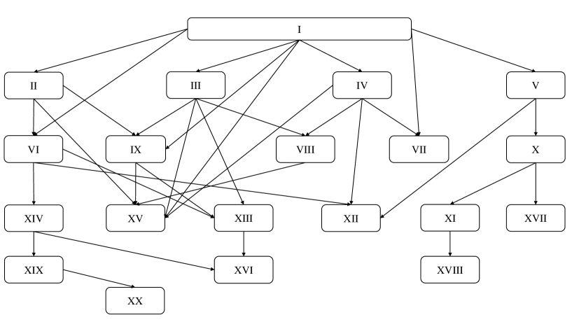
Figure 1: Contractions of semidegenerate systems. System $B$ is a Bôcher contraction of system $A$ provided there is an arrow pointed from $A$ to $B$.

7 Extensions of semi-degenerate Laplace systems to 4th order superintegrable systems

To compile this list we start with the “generic” 4th order system (6) and apply each Bôcher contraction to this system as described in subsection 4.2. In this case we have $n=3,h=6,k=5$. Since each of the 5 basic Bôcher contractions is not completely symmetric in the coordinates $x_{i}$ there are potentially $5!\times 5=120$ limits to take, though again this can be reduced substantially. Each contraction yields a superintegrable system but it need not be 4th order or an extension of a semidegenerate system. The contracted system will have 6 independent symmetries and $d$-parameter potential. If $d<5$ then the contraction cannot cover a full 4th order system so we do not count it. If $d=k=5$ but the contracted potential is functionally dependent, again the contraction cannot counted. If $d=5$ and the contracted potential is functionally independent but there are 5 linearly independent 2nd order symmetries the contracted system is 2nd order nondegenerate and cannot be counted. The remaining cases are 4th order systems with 4 2nd order symmetries. For each of these cases we must check if the system can be restricted to a 3-parameter system with 5 linearly independent symmetries. If so, we count it as an extension, though we ignore “identity“ contractions of (6) to itself. Once we have determined all new 4th order extensions resulting from Bôcher contractions of (6) we repeat the procedure for each of these new systems. We continue this process on the results until no new extension systems appear. We list the results:

1. System i: This is the extension (6) of semi-degenerate system I.

2. System ii: This is an extension of semi-degenerate system II.

   $$V_{F}=\frac{a_{0}}{\sqrt{x^{2}+y^{2}+z^{2}}}+\frac{a_{1}}{x^{2}}+\frac{a_{2}}{y^{2}}+\frac{a_{3}}{z^{2}}+a_{4}.$$

   It is a $\downarrow[2111]$ contraction of System i.

3. System iii: This is an extension of Systems IV and III. It is a $\downarrow[2111]$ contraction of System i.

   $$V_{F}:=\frac{a_{3}}{x^{2}}+\frac{a_{4}}{y^{2}}+\frac{a_{5}z}{y^{2}\ \sqrt{y^{2}+z^{2}}}+a_{1}-a_{2}(x^{2}+y^{2}+z^{2}).$$

4. System iv: This is an extension of System V, and a $\downarrow[221]$ contraction of System i.

   $$V_{F}=\frac{a_{2}}{(x+iy)^{2}}+a_{4}(x^{2}+y^{2}+z^{2})+a_{3}+\frac{a_{5}(x+iy)}{\sqrt{1-(x+iy)^{2}}}+\frac{a_{1}}{z^{2}}.$$

5. System v: This is an extension of System VI, a $\downarrow[2111]$ contraction of Systems i and ii, and a $\downarrow[311]$ contraction of System i.

   $$V_{F}=\frac{a_{3}}{x^{2}}+\frac{a_{1}}{y^{2}}+a_{2}+a_{4}z-a_{5}(x^{2}+y^{2}+z^{2}).$$

6. System vi: This is an extension of System VII, and a $\downarrow[221]$ contraction of Systems iii and iv.

   $$V_{F}=\frac{a_{2}}{(x+iy)^{2}}+a_{4}(x^{2}+y^{2}+z^{2})+a_{3}+a_{1}z+\frac{a_{5}(x+iy)}{\sqrt{1-(x+iy)^{2}}}.$$

7. System vii: This is an extension of System VIII, a $\downarrow[211]$ contraction of System iii, a $\downarrow[221]$ contraction of System iii, and a $\downarrow[311]$ contraction of System i.

   $$V_{F}=a_{3}+a_{1}x-a_{2}(4x^{2}+y^{2}+z^{2})+\frac{a_{4}}{z^{2}}+\frac{a_{5}y}{z^{2}\,\sqrt{y^{2}+z^{2}}}.$$

8. System viii: This is an extension of System IX, a $\downarrow[2111]$ contraction of Systems ii, iii and xvi, and a $\downarrow[221]$ contraction of Systems i and iii.

   $$V_{F}=\frac{a_{3}}{x^{2}}+\frac{a_{2}(y+iz)}{(y-iz)^{3}}+\frac{a_{1}}{(iy+z)^{2}}+\frac{a_{5}}{\sqrt{x^{2}+y^{2}+z^{2}}}+a_{4}.$$

   It is Stäckel equivalent to system

   $$V^{\prime}_{F}=\frac{a_{3}}{z^{2}}-a_{2}(x^{2}+y^{2}+z^{2})-a_{1}+\frac{a_{5}}{(x+iy)\ \sqrt{x^{2}+y^{2}}}+\frac{a_{4}}{(x+iy)^{2}}.$$

9. System ix: This is a $\downarrow[2111]$ contraction of System iv. It is an extension of System X.

   $$V_{F}=a_{1}+\frac{a_{2}}{z^{2}}+a_{3}x+a_{4}y+\frac{a_{5}}{\sqrt{x-iy}}.$$

10. System x: This is an extension of System VII, a $\downarrow[2111]$ contraction of Systems ii, iii and v, a $\downarrow[221]$ contraction of Systems i, ii, iii and v, a $\downarrow[311]$ contraction of System iii, and a $\downarrow[32]$ contraction of Systems i, iii and v.

    $$V_{F}=\frac{a_{2}(x-iz)}{(x+iz)^{3}}+\frac{a_{1}}{(x+iz)^{2}}+a_{3}+a_{5}y-a_{4}(x^{2}+y^{2}+x^{2}).$$

    It is Stäckel equivalent to system

    $$V^{\prime}_{F}=-a_{2}(x^{2}+y^{2}+z^{2})+a_{1}+\frac{a_{3}}{(x+iy)^{2}}+\frac{a_{5}z}{(x+iy)^{3}}+\frac{a_{4}(x-iy)}{(x+iy)^{3}}.$$

11. System xi: This is an extension of Systems XI and XII, a $\downarrow[2111]$ contraction of Systems iii and v, and a $\downarrow[311]$ contraction of Systems i, iii and v.

    $$V_{F}=\frac{a_{3}}{x^{2}}+a_{1}+a_{2}y-a_{5}(x^{2}+4y^{2}+z^{2})+a_{4}z.$$

12. System xii: This is an extension of System XIII, a $\downarrow[2111]$ contraction of System iv, and $\downarrow[2111]$, $[221]$ and $[41]$ contractions of Systems v.

    $$V_{F}=\frac{a_{4}}{(iy+z)^{3}}+\frac{a_{3}}{x^{2}}+\frac{a_{5}(y+iz)}{(y-iz)^{3}}+\frac{a_{2}}{(iy+z)^{2}}+a_{1}.$$

    Stäckel equivalent to

    $$V^{\prime}_{F}=a_{4}(x+iy)+\frac{a_{3}}{z^{2}}+a_{5}(x^{2}+y^{2}+z^{2})+a_{2}+\frac{a_{1}}{(x+iy)^{2}}.$$

13. System xiii: This is an extension of System XI, a $\downarrow[311]$ and $[32]$ contraction of System ii. A $\downarrow[221]$ contraction of Systems iii and iv, a $\downarrow[32]$ contraction of Systems i and iii, and a $\downarrow[2111]$ and $[32]$ contraction of System vii.

    $$V_{F}=a_{4}+\frac{a_{1}}{(x+iy)^{2}}+\frac{a_{3}z}{(x+iy)^{3}}+\frac{a_{2}(x^{2}+y^{2}-3z^{2})}{(x+iy)^{4}}+\frac{a_{5}}{\sqrt{x^{2}+y^{2}+z^{2}}}.$$

    It is Stäckel equivalent to

    $$V_{F}=\frac{a_{1}}{(x+iy)^{2}}+a_{2}+a_{3}z+a_{4}(x^{2}+y^{2}+4z^{2})+\frac{a_{5}}{(x+iy)\sqrt{x^{2}+y^{2}}}.$$

14. System xiv: This is a $\downarrow[41]$ contraction of Systems v and xii, and a $\downarrow[32]$ contraction of System xi. It is an extension of System XV.  $V_{F}=a_{1}+a_{2}z+$

    $$a_{3}(x+iy)+\frac{a_{4}}{(x+iy)^{2}}+a_{5}\left(3ix(z-y)+2z^{2}+2y^{2}-x^{2}-3xy\right).$$

15. System xv: This is a $\downarrow[2111]$ contraction of System xiii, and $\downarrow[2111]$ and $[32]$ contractions of System ix. It is an extension of System XVI.

    $$V_{F}=a_{1}+a_{2}x+a_{3}y+a_{4}z+\frac{a_{5}}{\sqrt{x-iy}}.$$

16. System xvi: This is an extension of system XV, a $\downarrow[221]$ and $[32]$ contraction of System v, $\downarrow[2111]$, $[221]$ and $[32]$ contractions of Systems xii, a $\downarrow[32]$ contraction of Systems i and iii, $\downarrow[2111]$, $[221]$ and $[32]$ contractions of System xii, $\downarrow[2111]$ and $[221]$ contractions of System xiv, and $\downarrow[2111]$, $[221]$ $[32]$ and $[41]$ contractions of System xi.

    $$V_{F}=a_{1}+a_{2}x+a_{3}(y+iz)+\frac{a_{4}}{(y+iz)^{2}}+a_{5}(4x^{2}+y^{2}+z^{2}).$$

17. System xvii: This is a $\downarrow[2111]$, $[311]$ and $[41]$ contraction of System xvi, a $\downarrow[2111]$, $[221]$ $[311]$, $[32]$ and $[41]$ contraction of Systems xiv and xv, a $\downarrow[311]$ and $[32]$ contraction of Systems x, v, and xxvi, a $\downarrow[311]$ contraction of Systems xii, vi and ix, a $\downarrow[41]$ contraction of System ix, a $\downarrow[32]$ contraction of System xiii, and $\downarrow[221]$, $[311]$, $[32]$ and $[41]$ contractions of System xi.

    $$V_{F}=a_{1}+a_{2}x+a_{3}y+a_{4}z+a_{5}(x+iz)^{2}.$$

Figures 2 and 3 depict the Bôcher contraction scheme for 4th order extensions of semidegenerate systems.

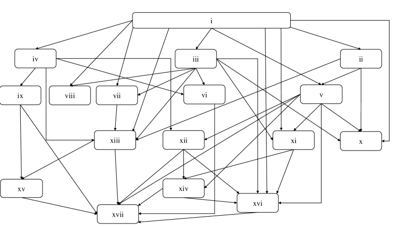
Figure 2: Contractions of 4th order systems that are extensions of semidegenerate systems

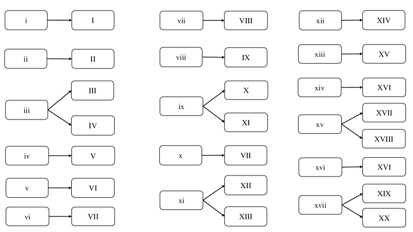
Figure 3: Extensions of semidegenerate systems

8 Conclusions and outlook

Using the powerful tool of Bôcher contractions we have found a family of 20 semidegenerate 2nd order 3D conformally superintegrable Laplace systems and 17 4th order conformally superintegrable Laplace systems that are extensions of these and have related them via Bôcher contractions. These correspond to about 100 Helmholtz systems on a variety of manifolds. These results apply to classical systems with only a few obvious adjustments. Every semidegenerate system extends to a 4th order system. Only the Bôcher contraction $[11111]\downarrow[5]$ fails to produce any new semidegenerate system. This work partially fills a gap in the classification of 3D 2nd order superintegrable systems.

The difficulty here is that, as yet, there is no detailed structure and classification theory for semidegenerate systems or for 4th order superintegrable systems. For nondegenerate 3D systems there is a complete theory with a guarantee that any Bôcher contraction of a nondegenerate system yields a nondegenerate system, unless the contracted potential is functionally dependent. Here we can use Bôcher contractions as a valuable calculational tool but with no guarantee of completeness. Is every semidegenerate system obtainable from (5) by a sequence of Bôcher contractions and Stäckel transforms? We suspect so but have no proof. Does every semidegenerate system extend to a 4th order superintegrable system? Again, we suspect so but have no proof. System ii and all systems obtained from it by contraction have a closed symmetry algebra. Is the symmetry algebra of i closed? We expect so but have not carried out the difficult calculation to verify this.

9 Acknowledgment

This work was partially supported by a grant from the Simons Foundation (#412351, Willard Miller, Jr) and by CONACYT grant (# 250881 to M.A. Escobar ).

References

• [1] Superintegrability in Classical and Quantum Systems, P. Tempesta, P. Winternitz , W. Miller, G. Pogosyan, editors, AMS, vol. 37, 2005, ISBN-10: 0-8218-3329-4, ISBN-13: 978-0-8218-3329-2
• [2] W. Miller Jr., S. Post and P. Winternitz. Classical and Quantum Superintegrability with Applications , J. Phys. A: Math. Theor., 46, 423001, (2013)
• [3] E. G. Kalnins , J. M. Kress , and W. Miller Jr., Second order superintegrable systems in conformally flat spaces. I: 2D classical structure theory. J. Math. Phys., 46, 053509, ( 2005); II: The classical 2D Stäckel transform. J. Math. Phys., 46, 053510, (2005); III. 3D classical structure theory, J. Math. Phys., 46, 103507, (2005), IV. The classical 3D Stäckel transform and 3D classification theory,, J. Math. Phys., 47, 043514, (2006) ; V: 2D and 3D quantum systems. J. Math. Phys., 47, 09350, (2006); Nondegenerate 2D complex Euclidean superintegrable systems and algebraic varieties, J. Phys. A: Math. Theor., 40, 3399-3411, (2007), http://dx.doi.org/10.1088/1751-8113/40/13/008.
• [4] E. G. Kalnins, J. M. Kress, W. Miller Jr and S. Post, Laplace-type equations as conformal superintegrable systems, Advances in Applied Mathematics 46 (2011) 396416.
• [5] J. J. Capel, J. M. Kress and S. Post, Invariant Classification and Limits of Maximally Superintegrable Systems in 3D, SIGMA, 11 (2015), 038, 17 pages arXiv:1501.06601 http://dx.doi.org/10.3842/SIGMA.2015.038
• [6] E. G. Kalnins, W. Miller Jr and E. Subag, Laplace equations, conformal superintegrability and Bôcher contractions, Acta Polytechnica, 56, 3, 214-223, 2016. http://arxiv.org/abs/1510.09067
• [7] E. G. Kalnins, W. Miller, Jr., and E. Subag, Bôcher contractions of conformally superintegrable Laplace equations, SIGMA, 12 (2016), 038, 31 pages;
• [8] J. J. Capel and J. M. Kress, Invariant Classification of Second-order Conformally Flat Superintegrable Systems, J. Phys. A: Math. Theor. 47 (2014), 495202.
• [9] N.W. Evans, Superintegrability in classical mechanics, Phys. Rev. A.   41, 5668-70, (1990).
• [10] E. G. Kalnins , J. M. Kress , and W. Miller Jr., Fine structure for 3D second order superintegrable systems: 3-parameter potentials, J. Phys. A: Math. Theor., 40, 5875-5892, (2007).
• [11] P. E. Verrier and N. W. Evans, A new superintegrable Hamiltonian, J. Math. Phys., 49 (2008), 022902, 8 pages, arXiv:0712.3677.
• [12] Y. Tanoudis and C. Daskaloyannis, Algebraic calculation of the energy eigenvalues for the nondegenerate three-dimensional Kepler-Coulomb potential, SIGMA, 7 (2011), 054, 11 pages, arXiv:1102.0397.
• [13] E. G. Kalnins , J. M. Kress , and W. Miller Jr., Extended Kepler-Coulomb quantum superintegrable systems in 3 dimensions, J. Phys. A: Math. Theor., 46, (2013) 085206.
• [14] M. A. Rodriguez, P. Tempesta and P. Winternitz, Reduction of superintegrable systems: The anisotropic harmonic oscillator,Phys. Rev. E, 78, 046608, (2008)
• [15] N. W. Evans and P. E. Verrier, Superintegrability of the caged anisotropic oscillator, J. Math. Phys., 49 (2008),092902, 10 pages, arXiv:0808.2146
• [16] M. A. Escobar-Ruiz and W. Miller, Jr., Conformal Laplace superintegrable systems in 2D: Polynomial invariant subspaces, J. Phys. A: Math. Theor., 49 305202, 2016.
• [17] E. Inönü and E. P. Wigner., On the contraction of groups and their representations. Proc. Nat. Acad. Sci. (US), 39, 510-524, (1953), http://dx.doi.org/10.1073/pnas.39.6.510
• [18] E. G. Kalnins and W. Miller Jr., Quadratic algebra contractions and 2nd order superintegrable systems, Anal. Appl. 12, 583-612, (2014), http://dx.doi.org/10.1142/S0219530514500377
• [19] M. Bôcher, Ueber die Reihenentwickelungen der Potentialtheorie, B. G. Teubner, Leipzig 1894.
• [20] M. A. Escobar-Ruiz, E. G. Kalnins, W. Miller, Jr. and E. Subag, Bôcher and abstract contractions of 2nd order quadratic algebras, arXiv:1611.02560 [math-ph], (submitted) 2016
• [21] F. R. Gantmacher, Matrix Theory, Volume 2, Chelsea, New York, 1960 (Translation of the Russian original).