Quantum-gravitational effects on gauge-invariant scalar and tensor perturbations during inflation: The slow-roll approximation

Abstract

We continue our study on corrections from canonical quantum gravity to the power spectra of gauge-invariant inflationary scalar and tensor perturbations. A direct canonical quantization of a perturbed inflationary universe model is implemented, which leads to a Wheeler-DeWitt equation. For this equation, a semiclassical approximation is applied in order to obtain a Schrödinger equation with quantum-gravitational correction terms, from which we calculate the corrections to the power spectra. We go beyond the de Sitter case discussed earlier and analyze our model in the first slow-roll approximation, considering terms linear in the slow-roll parameters. We find that the dominant correction term from the de Sitter case, which leads to an enhancement of power on the largest scales, gets modified by terms proportional to the slow-roll parameters. A correction to the tensor-to-scalar ratio is also found at second order in the slow-roll parameters. Making use of the available experimental data, the magnitude of these quantum-gravitational corrections is estimated. Finally, the effects for the temperature anisotropies in the cosmic microwave background are qualitatively obtained.

I Introduction

The search for a theory of quantum gravity will only be successful if one eventually finds a way to test the candidate theories by experiment or observation oup ; KK12 . Because of the extremely high energies at which quantum-gravitational effects are expected to be strong, many researchers have looked for features of quantum-gravitational origin in the anisotropies of the cosmic microwave background (CMB); see, for example, KK-PRL ; BEKKP ; Gianluca ; BE14 ; ACT06 ; Sasha1 ; Sasha2 ; Sasha3 ; KTV16 ; AAN ; MO16 ; BGS15 ; SBB16 ; AG16 . These anisotropies are thought to originate during the inflationary phase of the primordial universe from quantum fluctuations of the metric and the scalar inflaton field. Hence, they are in a sense already a consequence of the quantum nature of space-time and thus an effect of quantum gravity. What we are going to study in the following is to derive the corrections that arise from quantizing the Universe as a whole in the canonical formalism that leads to the Wheeler-DeWitt equation.

One way to obtain corrections to the power spectra of the inflationary scalar and tensor perturbations, which lead to the CMB anisotropies, is to perform a semiclassical approximation of the Wheeler-DeWitt equation singh . This procedure leads to a Schrödinger equation with quantum-gravitational correction terms, which can be used to calculate the corrected power spectra. This was analyzed for a simple model containing only non-gauge-invariant perturbations of a scalar field in KK-PRL ; BEKKP ; Gianluca . An alternative semiclassical approximation was presented in bertoni and was used to calculate CMB corrections in BE14 ; ACT06 ; Sasha1 ; Sasha2 ; Sasha3 ; KTV16 . The results of both approaches were essentially the same, with differences only in the numerical factors.

We have previously studied the corrections to the power spectra of gauge-invariant scalar and tensor perturbations and have made explicit calculations for the de Sitter case BKK . Here, we shall extend our analysis and use a generic slow-roll approximation that is compatible with all observational data obtained so far and which encompasses a wide range of inflaton potentials.

Our paper is organized as follows. In Sec. II, we summarize the quantization procedure and the semiclassical approximation. This leads to the equations we use in Sec. III to obtain general expressions for the power spectra without and with quantum gravity corrections. In Sec. IV, we introduce the slow-roll approximation, and in Sec. V we calculate the corresponding uncorrected power spectra. Sec. VI represents the main part of the paper; here, we calculate the slow-roll power spectra with the quantum-gravitational corrections. In Sec. VII, we derive from this the corrections to the spectral index, its running, and to the tensor-to-scalar ratio. We also comment on the observability of the calculated effects and compute the correction for the CMB temperature anisotropies. Finally, in Sec. VIII, we summarize and perform an outlook. We also compare our results with the results obtained in KTV16 .

II Quantization and semiclassical approximation of a perturbed inflationary universe

Here and in the next section, we present a brief self-contained summary of our earlier results from BKK . We model an inflationary universe as a flat Friedmann-Lemaître-Robertson-Walker (FLRW) space-time plus fluctuations. The matter content is supposed to be a massive scalar inflaton field $\phi$ with potential $\mathcal{V}(\phi)$, and a vanishing cosmological constant is assumed. For convenience, we will use conformal time $\eta$, which is defined in terms of the cosmic time $t$ and the scale factor $a(t)$ by ${\mathrm{d}\eta}/{\mathrm{d}t}=a^{-1}$. Furthermore, introducing four space-time functions $A$, $B$, $\psi$, $E$ to describe the scalar perturbations, as well as the symmetric spatial tensor $h_{ij}$ to encode the tensorial degrees of freedom, the metric of the FLRW space-time plus fluctuations reads (see, for example, Mukhanov:1992 ; PU09 )

$$\mathrm{d}s^{2}=a^{2}(\eta)\Bigl{\{} -\left(1-2A\right)\mathrm{d}\eta^{2}+2\left(\partial_{i}B\right)\mathrm{d}x^{i}\mathrm{d}\eta$$ (1)

$$+\left[\left(1-2\psi\right)\delta_{ij}+2\partial_{i}\partial_{j}E+h_{ij}\right]\mathrm{d}x^{i}\mathrm{d}x^{j}\Bigr{\}}\,.$$

The additional scalar perturbations $\varphi(\eta,\mathbf{x})$ of the field $\phi$ can be combined with the scalar metric perturbations to construct a master gauge-invariant quantity called the Mukhanov-Sasaki variable Mukhanov:1992 ; PU09 :

$$v(\eta,\mathbf{x}):=a\left[\varphi+\frac{\phi^{\prime}}{\mathscr{H}}\left(A+2\,\mathscr{H}\left(B-E^{\prime}\right)+\left[B-E^{\prime}\right]^{\prime}\right)\right],$$ (2)

where we have indicated the derivative with respect to $\eta$ with a prime and used the definition $\mathscr{H}:=a^{\prime}/a$.

We denote the Fourier transform of (2) as $v_{\mathbf{k}}$ and also introduce the Fourier-transformed perturbation variable of the gauge-invariant tensor perturbations $h_{ij}$ with polarization $\lambda\in\{+,\times\}$ as

$$v_{\mathbf{k}}^{(\lambda)}:=\frac{a\,h^{(\lambda)}_{\mathbf{k}}}{\sqrt{16\pi G}}.$$ (3)

We note that an important feature in the definition of these variables is the rescaling with respect to $a$.

The action $S$ for our perturbed inflationary universe then takes the form

$$S=\frac{1}{2}\int\mathrm{d}\eta\,\Biggl{\{}\,\mathfrak{L}^{3} \left[-\,\frac{3}{4\pi G}\,(a^{\prime})^{2}+a^{2}\,(\phi^{\prime})^{2}-2\,a^{4}\,\mathcal{V}(\phi)\right]$$

$$+\,\frac{1}{\mathfrak{L}^{3}}\sum_{\mathbf{k}} \,\Bigl{[}v_{\mathbf{k}}^{\prime}{v_{\mathbf{k}}^{*}}^{\prime}+{}^{\text{S}}\omega^{2}_{\mathbf{k}}\,v_{\mathbf{k}}v_{\mathbf{k}}^{*}\Bigr{]}\Biggr{.}$$

$$+\,\frac{1}{\mathfrak{L}^{3}}\sum_{\lambda=+,\times}\sum_{\mathbf{k}} \left[v_{\mathbf{k}}^{(\lambda)\prime}v_{\mathbf{k}}^{(\lambda)*\prime}+{}^{\text{T}}\omega^{2}_{\mathbf{k}}\,v_{\mathbf{k}}^{(\lambda)}v_{\mathbf{k}}^{(\lambda)*}\right]\Biggr{\}}\,.$$ (4)

Here, we have introduced the “frequencies” ${}^{\text{S}}\omega$ and ${}^{\text{T}}\omega$ by

$${}^{\text{S}}\omega^{2}_{\mathbf{k}}(\eta):=k^{2}-\frac{z^{\prime\prime}}{z}\,,\quad{}^{\text{T}}\omega^{2}_{\mathbf{k}}(\eta):=k^{2}-\frac{a^{\prime\prime}}{a}\,,$$ (5)

where $z$ is defined as $z:=a\,\phi^{\prime}/\mathscr{H}$.

In order to avoid the infinity arising from the volume integral of the action, it is necessary to introduce a maximum length scale $\mathfrak{L}$, which can be thought of as the maximum size of the universe under consideration (see e.g. the Appendix of Parker:2009 ). We will later have to specify a value for $\mathfrak{L}$ when comparing our results to observations; however, up to that point it is possible to remove $\mathfrak{L}$ from the notation by applying the following redefinitions Sasha2 ; BKK :

$$a_{\text{new}}=a_{\text{old}}\,\mathfrak{L}\,,\;\eta_{\text{new}}=\frac{\eta_{\text{old}}}{\mathfrak{L}}\,,\;k_{\text{new}}=k_{\text{old}}\,\mathfrak{L}\,,\;v_{\text{new}}=\frac{v_{\text{old}}}{\mathfrak{L}^{2}}\,.$$ (6)

Note that, after these rescalings, $a$ obtains the dimension of a length, whereas $\eta$, $k$, and $v_{\mathbf{k}}$ are dimensionless.

In order to perform an entirely consistent quantization, one should use a real set of variables instead of the complex $v_{\mathbf{k}}$ variables. Such real variables can be constructed from a double copy of the complex variables and the wave function, see, for instance, Martin:2012 . Nonetheless, since such a redefinition will not influence our calculations later on, we will not introduce these new variables and thus treat $v_{\mathbf{k}}$ as if it were real in order to keep our presentation brief and concise.

After a canonical quantization oup of (II), and choosing a product ansatz for the full wave function, we end up with a Wheeler-DeWitt equation of the following form, for each mode $\mathbf{k}$ and for both the scalar and tensor perturbations,

$$\frac{1}{2}\Biggl{\{}\mathrm{e}^{-2\alpha}\biggl{[} \frac{1}{m_{\text{P}}^{2}}\,\frac{\partial^{2}}{\partial\alpha^{2}}-\frac{\partial^{2}}{\partial\phi^{2}}+2\,\mathrm{e}^{6\alpha}\,\mathcal{V}(\phi)\biggr{]}$$

$$-\,\frac{\partial^{2}}{\partial v_{\mathbf{k}}^{2}}+\omega^{2}_{\mathbf{k}}(\eta)\,v_{\mathbf{k}}^{2}\Biggr{\}}\Psi_{\mathbf{k}}(\alpha,\phi,v_{\mathbf{k}})=0\,.$$ (7)

We have combined the notation for the scalar and tensor modes and thus removed the superscripts S, T and $(\lambda)$. We also have set (besides $c=1$) $\hbar=1$ and introduced the dimensionless quantity $\alpha:=\ln\!\left(a/a_{0}\right)$, where $a_{0}$ is a reference scale factor. For simplicity, we will not write out this reference scale in the following (or, equivalently, $a_{0}=1$ will be imposed); but it is implicitly understood that a factor $a_{0}$ is associated with every factor of $\mathrm{e}^{\alpha}$. We have also defined a rescaled Planck mass $m_{\text{P}}$ in order to incorporate several numerical prefactors,

$$m_{\text{P}}^{2}:=\frac{3}{4\pi G}\,.$$ (8)

We shall use $m_{\text{P}}^{2}$ as the parameter with respect to which the semiclassical approximation of (II) is carried out singh ; KK-PRL . For this purpose, $\phi$ has to be rescaled to the dimensionless variable

$$\tilde{\phi}:=m_{\mathrm{P}}^{-1}\phi.$$ (9)

More precisely, the reason behind this rescaling is that we will subsequently perform an expansion in inverse powers of $m_{\mathrm{P}}$ and, in order to obtain the correct classical background equations at first order in that expansion, it is necessary that the first two terms in square brackets of (II) have the same power of $m_{\mathrm{P}}$. In any case, once the expansion is made, we will revert and provide all expressions in terms of $\phi$.

The approximation is then performed by expanding the wave function $\Psi_{\mathbf{k}}$ using the functions $S_{i}(\alpha,\tilde{\phi},v_{\mathbf{k}})$, $i=0,1,2,\dots$, as follows:

$$\Psi_{\mathbf{k}}=\exp\Bigl{[}\mathrm{i}\left(m_{\rm P}^{2}\,S_{0}+m_{\rm P}^{0}\,S_{1}+m_{\rm P}^{-2}\,S_{2}+\ldots\right)\Bigr{]}.$$ (10)

After inserting this WKB-type ansatz into (II), the terms containing a certain power of $m_{\rm P}$ are collected and their sum is set equal to zero.

At order $m_{\text{P}}^{2}$, we obtain the Hamilton-Jacobi equation of the minisuperspace background,

$$-\left(\frac{\partial S_{0}}{\partial\alpha}\right)^{2}+m_{\rm P}^{2}\left(\frac{\partial S_{0}}{\partial\phi}\right)^{2}+\frac{2\,\mathrm{e}^{6\alpha}}{m_{\rm P}^{2}}\,\mathcal{V}(\phi)=0\,.$$ (11)

The Planck mass occurs explicitly here because the expansion in (II) is performed in the form of the equation using $\tilde{\phi}$ instead of $\phi$.

At the next order, $m_{\mathrm{P}}^{0}$, it is possible to write the corresponding equation for $S_{1}$ as a Schrödinger equation for a related wave function $\psi^{(0)}_{\mathbf{k}}$ in the following way,

$$\mathcal{H}_{\mathbf{k}}\psi^{(0)}_{\mathbf{k}}=\mathrm{i}\,\frac{\partial}{\partial\eta}\,\psi^{(0)}_{\mathbf{k}},$$ (12)

where the conformal time is defined in terms of the minisuperspace variables by

$$\frac{\partial}{\partial\eta}:=\mathrm{e}^{-2\alpha}\left[-\,\frac{\partial S_{0}}{\partial\alpha}\frac{\partial}{\partial\alpha}+m_{\rm P}^{2}\,\frac{\partial S_{0}}{\partial\phi}\frac{\partial}{\partial\phi}\right],$$ (13)

and the perturbative Hamiltonian operator is given as follows,

$$\mathcal{H}_{\mathbf{k}}:=-\,\frac{1}{2}\,\frac{\partial^{2}}{\partial v_{\mathbf{k}}^{2}}+\frac{1}{2}\,\omega^{2}_{\mathbf{k}}(\eta)\,v_{\mathbf{k}}^{2}.$$ (14)

The information at the next order, $m_{\mathrm{P}}^{-2}$, can be encoded in a wave function $\psi^{(1)}_{\mathbf{k}}$, related to the function $S_{2}$, which obeys the following corrected Schrödinger equation:

$$\mathrm{i}\,\frac{\partial}{\partial\eta}\,\psi^{(1)}_{\mathbf{k}}=\mathcal{H}_{\mathbf{k}}\psi^{(1)}_{\mathbf{k}}-\frac{\psi^{(1)}_{\mathbf{\mathbf{k}}}}{2\,m_{\rm P}^{2}\,\psi^{(0)}_{\mathbf{k}}} \Biggl{[}\frac{\bigl{(}\mathcal{H}_{\mathbf{k}}\bigr{)}^{2}}{V}\,\psi^{(0)}_{\mathbf{k}}$$ (15)

$$+\mathrm{i}\,\frac{\partial}{\partial\eta}\!\left(\frac{\mathcal{H}_{\mathbf{\mathbf{k}}}}{V}\right)\psi^{(0)}_{\mathbf{k}}\Biggr{]}\,.$$

Here, we have defined an auxiliary potential as

$$V(a,\phi):=\frac{2\,a^{4}}{m_{\rm P}^{2}}\,\mathcal{V}(\phi),$$ (16)

which has the dimension of a length squared.

In summary, the most important relations of this section are the two wave equations (12) and (15). The former one describes quantum fluctuations evolving on a classical (FLRW) background space-time, while the latter one encodes also corrections arising from the quantum behavior of that background. The aim of this paper is thus to solve these two equations with relevant initial conditions in order to obtain the power spectra with quantum-gravitational corrections for inflationary perturbations. In the next section, the ansatz to be used for such a purpose is described, as well as the explicit form of the power spectra.

III Gaussian ansatz and expressions for the power spectra

We use a Gaussian ansatz for both the uncorrected Schrödinger equation (12) and the corrected one (15), with the normalization factor $N_{\mathbf{k}}^{(0,1)}(\eta)$ and the inverse Gaussian widths $\Omega_{\mathbf{k}}^{(0,1)}(\eta)$ BKK ,

$$\psi^{(0,1)}_{{\mathbf{k}}}(\eta,v_{\mathbf{k}})=N_{\mathbf{k}}^{(0,1)}(\eta)\,\text{e}^{-\frac{1}{2}\,\Omega_{\mathbf{k}}^{(0,1)}(\eta)\,v_{\mathbf{k}}^{2}}.$$ (17)

Here, and in the following, the superscript $(0)$ stands for the uncorrected and $(1)$ for the corrected case. As will be shown below, in order to obtain the power spectra for the scalar and tensor perturbations, we have to find the solutions for $\Omega_{\mathbf{k}}^{(0,1)}$. For the uncorrected Schrödinger equation, we have to solve

$$\mathrm{i}\,\Omega_{\mathbf{k}}^{(0)\prime}(\eta)=\bigl{(}\Omega_{\mathbf{k}}^{(0)}(\eta)\bigr{)}^{2}-\omega^{2}_{\mathbf{k}}(\eta)\,,$$ (18)

while for the corrected Schrödinger equation, we have to find a solution to

$$\mathrm{i}\,\Omega_{\mathbf{k}}^{(1)\prime}(\eta)=\bigl{(}\Omega_{\mathbf{k}}^{(1)}(\eta)\bigr{)}^{2}-\widetilde{\omega}^{2}_{\mathbf{k}}(\eta).$$ (19)

In this last expression the corrected frequencies $\widetilde{\omega}_{\mathbf{k}}$ have been defined as follows:

$$\widetilde{\omega}_{\mathbf{k}}^{2}:=\omega_{\mathbf{k}}^{2}-\frac{1}{2m_{\mathrm{P}}^{2}V}\,\Re\!\kern 0.83328pt\mathfrak{e}\kern 0.83328pt\biggl{[} \left(3\Omega^{(0)}_{\mathbf{k}}-{\rm i}\,(\ln V)^{\prime}\right)\left(\omega^{2}_{\mathbf{k}}-(\Omega^{(0)}_{\mathbf{k}})^{2}\right)$$ (20)

$$+2\,\mathrm{i}\,\omega_{\mathbf{k}}\,\omega^{\prime}_{\mathbf{k}}\biggr{]}.$$

As is explicitly written in this definition, in this paper we will only consider the real part of the correction terms for the frequencies, since the imaginary part tends to exhibit unphysical behavior, in particular unitarity violation. The presence of this term can be traced back to the fact that the starting point is the Wheeler-DeWitt equation, not the Schrödinger equation. Its treatment is subtle and not fully understood. Such a term can be relevant for calculating the probability of cosmological instabilities deSitter , but we do not expect it to play a role for the corrections of the power spectrum. For a more detailed discussion about this point we refer the reader to BKK .

Since the equation for $\Omega^{(1)}_{\mathbf{k}}$ is nonlinear, it is reasonable to linearize it around the background solution $\Omega^{(0)}_{\mathbf{k}}$ by defining $\widetilde{\Omega}^{(1)}_{\mathbf{k}}:=\Omega^{(1)}_{\mathbf{k}}-\Omega^{(0)}_{\mathbf{k}}$. After neglecting the quadratic term, one obtains the following linear equation:

$${\rm i}\,\widetilde{\Omega}^{(1)\prime}_{\mathbf{k}} = 2\,\Omega^{(0)}_{\mathbf{k}}\widetilde{\Omega}^{(1)}_{\mathbf{k}}-\left(\widetilde{\omega}^{2}_{\mathbf{k}}-\omega^{2}_{\mathbf{k}}\right).$$ (21)

Since it is usually possible to find an analytical solution for $\Omega^{(0)}_{\mathbf{k}}$, one is then left with only a linear equation for $\widetilde{\Omega}^{(1)}_{\mathbf{k}}$, which is easier to solve than the full non-linear equation (19).

Apart from the equations themselves, another important key aspect of the analysis is to choose appropriate and meaningful initial conditions. For the uncorrected case, as it is usually done in quantum field theory, the Bunch-Davies vacuum will be chosen, which in this setting means $\Omega^{(1)}_{{\mathbf{k}}}=k$. The case of an initial non-Bunch-Davies state was recently discussed in Broy16 . Moreover, as we have discussed in BKK , the most natural initial conditions for the corrected case should be those that best resemble the properties of the Bunch-Davies vacuum. Namely, when the mode is well inside its Hubble radius, it should be oscillating with a fixed constant frequency and amplitude. This is achieved by choosing

$$\Re\!\kern 0.83328pt\mathfrak{e}\kern 0.83328pt(\Omega^{(1)}_{{\mathbf{k}}})^{2} = \Re\!\kern 0.83328pt\mathfrak{e}\kern 0.83328pt(\widetilde{\omega}^{2}_{{\mathbf{k}}}),$$

$$\Im\mathfrak{m}\kern 0.83328pt(\Omega^{(1)}_{{\mathbf{k}}}) = 0.$$ (22)

Since the imaginary part of the corrected frequencies has been neglected, these two relations can simply be written as $\Omega^{(1)}_{{\mathbf{k}}}=\widetilde{\omega}_{{\mathbf{k}}}$. For the linearized function the above conditions are rewritten as $\widetilde{\Omega}^{(1)}_{{\mathbf{k}}}=k-\widetilde{\omega}_{{\mathbf{k}}}$. Therefore, the latter is the condition that will be used as initial data at early times ($\eta\rightarrow-\infty$).

The power spectrum for the scalar perturbations including the quantum-gravitational corrections is given by

$${\cal P}_{\text{S}}^{(1)}(k)=\frac{4\pi G}{a^{2}\,\epsilon}\,\frac{k^{3}}{2\pi^{2}}\,\frac{1}{2\,\Re\!\kern 0.83328pt\mathfrak{e}\kern 0.83328pt{}^{{}^{\text{S}}\!}\Omega_{\mathbf{k}}^{(1)}}\approx{\cal P}_{\text{S}}^{(0)}(k)\Big{\{}1+\Delta_{\text{S}}\Big{\}}\,,$$ (23)

where $\epsilon$ is the slow-roll parameter defined below in (28), and ${\cal P}_{\text{S}}^{(0)}(k)$ is the usual scalar power spectrum defined by inserting $\Omega^{(0)}_{\mathbf{k}}$ instead of $\Omega^{(1)}_{\mathbf{k}}$ into this expression. The quantum-gravitational effects are thus encoded in the term

$$\Delta_{\text{S}}:=-\,\frac{\Re\!\kern 0.83328pt\mathfrak{e}\kern 0.83328pt{}^{{}^{\text{S}}\!}\widetilde{\Omega}^{(1)}_{\mathbf{k}}}{\Re\!\kern 0.83328pt\mathfrak{e}\kern 0.83328pt{}^{{}^{\text{S}}\!}\Omega^{(0)}_{\mathbf{k}}}.$$ (24)

This ratio has to be computed in the limit of super-Hubble scales (or late times), given by $k\eta\rightarrow 0^{-}$, when the perturbations get “frozen”.

The power spectrum for the tensor perturbations is, consequently, obtained by

$${\cal P}_{\text{T}}^{(1)}(k)=\,\frac{64\pi G}{a^{2}}\,\frac{k^{3}}{2\pi^{2}}\,\frac{1}{2\,\Re\!\kern 0.83328pt\mathfrak{e}\kern 0.83328pt{}^{{}^{\text{T}}\!}\Omega^{(1)}_{\mathbf{k}}}\approx{\cal P}_{\text{T}}^{(0)}(k)\Big{\{}1+\Delta_{\text{T}}\Big{\}}\,.$$ (25)

Here, the same comment as in the scalar case about taking the super-Hubble scale limit for $\Re\!\kern 0.83328pt\mathfrak{e}\kern 0.83328pt\Omega_{\mathbf{k}}$ applies, and the corrections are given by the term

$$\Delta_{\text{T}}:=-\frac{\Re\!\kern 0.83328pt\mathfrak{e}\kern 0.83328pt{}^{{}^{\text{T}}\!}\widetilde{\Omega}^{(1)}_{\mathbf{k}}}{\Re\!\kern 0.83328pt\mathfrak{e}\kern 0.83328pt{}^{{}^{\text{T}}\!}\Omega^{(0)}_{\mathbf{k}}}.$$ (26)

Finally, the corrected tensor-to-scalar ratio $r^{(1)}$ is defined as

$$r^{(1)}:=\frac{{\cal P}_{\text{T}}^{(1)}(k)}{{\cal P}_{\text{S}}^{(1)}(k)}\approx r^{(0)}\left(1+\Delta_{\text{T}}-\Delta_{\text{S}}\right),$$ (27)

where $r^{(0)}$ is the ratio found at the order of approximation that corresponds to quantum field theory on a fixed, curved background. In the de Sitter case, since ${}^{\text{S}}\widetilde{\omega}_{\mathbf{k}}={}^{\text{T}}\widetilde{\omega}_{\mathbf{k}}$, both corrections are the same, $\Delta_{\text{T}}=\Delta_{\text{S}}$, and thus in our previous work BKK there appeared no correction to this quantity at the considered order of approximation. This will be different here.

To recap, note that the task of obtaining quantum-gravitational corrections to the scalar and tensor power spectra reduces to solving equation (21) with initial data (22). Once this is done, one only needs to compute the corresponding power spectra using the relations (23) and (25).

IV The slow-roll approximation

In this section the well-known slow-roll approximation is described in order to clarify and set up the notation. In addition, several physical quantities, which appear in the key equations of motion (18) and (21), will be explicitly given up to linear order in the slow-roll parameters, which we will define below.

Using the Hubble parameter $H=\dot{a}/{a}$, we can define the first slow-roll parameters $\epsilon$ and $\delta$ (see e.g. Eqs (8.37) and (8.38) in PU09 ),

$$\epsilon :=-\,\frac{\dot{H}}{H^{2}}=1-\frac{\mathscr{H}^{\prime}}{\mathscr{H}^{2}}\,,$$ (28)

$$\delta :=\epsilon-\frac{\dot{\epsilon}}{2H\epsilon}=-\,\frac{\ddot{\phi}}{H\dot{\phi}}\,.$$ (29)

In terms of the slow-roll parameter $\epsilon$, the equation $\dot{a}=Ha$ and the Hamiltonian constraint equation can be written as follows:

$$\frac{\ddot{a}}{a} =(1-\epsilon)\,H^{2}\,,$$ (30)

$$H^{2}\left(1-\frac{\epsilon}{3}\right) =\frac{2}{m_{\text{P}}^{2}}\,{\cal V}(\phi),$$ (31)

or, using the conformal time $\eta$,

$$\frac{a^{\prime\prime}}{a} =(2-\epsilon)\,{\mathscr{H}}^{2}\,,$$ (32)

$${\mathscr{H}}^{2}\left(1-\frac{\epsilon}{3}\right) =\frac{2a^{2}}{m_{\text{P}}^{2}}\,{\cal V}(\phi).$$ (33)

No approximation has been assumed yet, so these relations are exact.

The first order of our approximation scheme employs the function $S_{0}$, which satisfies the Hamilton-Jacobi equation (11) of the background. One cannot write down, of course, a general solution of (11) for general $\epsilon$ and thus for general potential ${\mathcal{V}}(\phi)$. But it is possible to recover (31) from the Hamilton-Jacobi equation (11) in the slow-roll approximation, in which terms quadratic and higher of $\epsilon$ and $\delta$ are neglected. At this level of approximation, we find

$$S_{0}=-\,\frac{a^{3}}{m_{\text{P}}}\,\sqrt{\frac{2}{3}\,\frac{\mathcal{V}(\phi)}{3-\epsilon(\phi)}},$$ (34)

where

$$\epsilon(\phi)=\frac{m_{\rm P}^{2}}{12{\mathcal{V}}^{2}}\left(\frac{\partial{\mathcal{V}}}{\partial\phi}\right)^{2}.$$ (35)

This is a well-known expression for $\epsilon$; see, for example, Eq. (8.49) in PU09 . Note that the sign of $S_{0}$ is not fixed by (11), and it is chosen such that the flux of time (13) points in the direction of the expansion of the universe.

Let us now introduce in more detail the slow-roll approximation. It essentially consists in assuming

$$\dot{\phi}^{2}\ll{\mathcal{V}}\,,\quad\ddot{\phi}\ll 3H\dot{\phi}\,.$$ (36)

It can be shown that this is equivalent to assuming that the slow-roll parameters $\epsilon$ and $\delta$ are small: $\epsilon\ll 1$ and $|\delta|\ll 1$. If one assumes those to be vanishing, one would recover the de Sitter case analyzed in our previous paper BKK . Since the pure de Sitter case is often too restrictive to make contact with observations, we shall now consider the first-order slow-roll approximation, which assumes $\epsilon$ and $\delta$ to be small but nonvanishing, and drop quadratic terms in those.

In order to solve the equations presented in the previous section in this approximation, we need to express the frequencies (5) and (20), as well as the potential (16) in terms of the conformal time $\eta$ and the slow-roll parameters $\epsilon$ and $\delta$.

It is well known (see e.g. PU09 ) that, in this approximation, the frequencies of the modes can be written as

$${}^{\text{S}}\omega^{2}_{\mathbf{k}}(\eta) = k^{2}-\frac{2+3\gamma}{\eta^{2}}+{\cal O}(2),$$ (37)

$${}^{\text{T}}\omega^{2}_{\mathbf{k}}(\eta) = k^{2}-\frac{2+3\epsilon}{\eta^{2}}+{\cal O}(2),$$ (38)

where ${\cal O}(2)$ stands for terms quadratic in $\epsilon$ and $\delta$ and where we have defined, for later convenience, the combination

$$\gamma:=2\epsilon-\delta.$$ (39)

Note that setting $\delta=\epsilon$, or equivalently $\gamma=\epsilon$, converts the equation for scalar perturbations into the one for tensor perturbations. Therefore we will perform all calculations only for the scalar perturbations and obtain the results for the tensor perturbations using this relation at the end.

Making use of the Hamiltonian constraint as written in (31), it is possible to write the rescaled potential (16) as

$$V=a^{4}H^{2}\left(1-\frac{\epsilon}{3}\right).$$ (40)

In order to write this expression explicitly in terms of the conformal time and the slow-roll parameters, we use the definition of the Hubble factor in terms of the conformal time to write

$$\eta=\int\frac{\mathrm{d}a}{a^{2}H}.$$ (41)

Integrating this relation by parts twice, we get

$$\eta=-\frac{(1+\epsilon)}{aH}+{\cal O}(2).$$ (42)

Now we can express the Hubble parameter as $H=a^{\prime}/a^{2}$ and integrate this equation, which leads to

$$a=\frac{C}{(-\eta)^{1+\epsilon}}+{\cal O}(2),$$ (43)

with an integration constant $C$. The Hubble parameter then takes the form

$$H=H_{0}\left(\frac{\eta}{\eta_{0}}\right)^{\epsilon}+{\cal O}(2)=H_{0}\left[1+\epsilon\ln\!\left(\frac{\eta}{\eta_{0}}\right)\right]+{\cal O}(2),$$ (44)

in which the constant $C$ has been replaced by

$$C=(1+\epsilon)\,\frac{(-\eta_{0})^{\epsilon}}{H_{0}};$$ (45)

$H_{0}$ being the value of the Hubble parameter at $\eta=\eta_{0}$. Physically, $H_{0}$ defines the de Sitter space-time we are considering as our reference. Below we will have to choose a value for $H_{0}$, since the results will depend on it. The only physically meaningful point that exists in the evolution of different modes, is when they cross the Hubble horizon. Therefore, we will choose $H_{0}$ as the value of the Hubble factor at the Hubble-scale exit, that is, $H_{0}=H_{k}$, with $H_{k}=k/a$. Following relation (42), this implies choosing $\eta_{0}=-1/k$ on the right-hand side of (44). (Note that in this equation, at the level of approximation chosen, $\eta_{0}$ is only meaningful at order $\epsilon^{0}$.) This choice makes both $H_{0}$ and $\eta_{0}$ become $k$-dependent but, since the evolution of every $k$-mode is independent, there is no problem in assuming that they experience a different reference de Sitter space-time.

As a side remark, note that the present approximation is valid during times $\eta$ which obey

$$|\eta_{0}|\mathrm{e}^{-1/\epsilon}\ll|\eta|\ll|\eta_{0}|\mathrm{e}^{1/\epsilon}.$$ (46)

Due to the smallness of $\epsilon$, this time range is very large. Nonetheless, when considering the asymptotic value for different physical objects as $\eta\rightarrow-\infty$, one should take into account that in this limit the approximation breaks down.

Finally, making use of all above results, the potential $V$ can be written in the following way:

$$V = \frac{(aH)^{4}}{H^{2}}\left(1-\frac{\epsilon}{3}\right)$$

$$= \frac{1}{H_{k}^{2}\eta^{4}(k\eta)^{2\epsilon}}\left(1+\frac{11\epsilon}{3}\right)+{\cal O}(2),$$

where $\eta_{0}$ has already been replaced by its value at horizon crossing. This expression can then be used in (20) to obtain the explicit form of the corrected frequencies at first order in the slow-roll parameters. In this way, we can already write our main equations, (18) and (21), at this level of approximation.

V Uncorrected power spectra

In this section, we will obtain the solution to Eq. (18), in order to construct the power spectra for scalar and tensor perturbations at the level of approximation that corresponds to the usual formalism of quantum field theory on classical background space-times. In Martin:2012 , one can find a detailed computation in a formalism very similar to the present one.

Considering for now only scalar perturbations, the solution to Eq. (18) with ${}^{\text{S}}\omega^{2}_{\mathbf{k}}$ given by (37) can be written as follows:

$${}^{\text{S}}\Omega_{\mathbf{k}}^{(0)}(\eta)=-\,\mathrm{i}\,\frac{{}^{\text{S}}y^{(0)\prime}_{\mathbf{k}}(\eta)}{{}^{\text{S}}y^{(0)}_{\mathbf{k}}(\eta)},$$ (48)

where the mode functions ${}^{\text{S}}y^{(0)}_{\mathbf{k}}$ can be expressed in terms of the Bessel functions $J_{\nu}$:

$${}^{\text{S}}y^{(0)}_{\mathbf{k}}=(-k\eta)^{1/2}\bigl{[} c_{{\mathbf{k}},1}\,J_{-(\gamma+3/2)}(-k\eta)$$

$$+c_{{\mathbf{k}},2}\,J_{\gamma+3/2}(-k\eta)\bigr{]}.$$ (49)

In order to obtain the Bunch-Davies vacuum for $\eta\rightarrow-\infty$, and choosing the usual normalization of the Wronskian

$${}^{\text{S}}y^{(0)\prime}_{\mathbf{k}}\,{}^{\text{S}}y^{(0)*}_{\mathbf{k}}-{}^{\text{S}}y^{(0)\prime*}_{\mathbf{k}}\,{}^{\text{S}}y^{(0)}_{\mathbf{k}}=\mathrm{i}\,,$$ (50)

it is necessary to set

$$c_{{\mathbf{k}},1} =-c_{{\mathbf{k}},2}\,{\rm e}^{-\mathrm{i}\pi(\gamma+3/2)},$$ (51)

$$c_{{\mathbf{k}},2} =-\frac{\mathrm{i}}{2}\sqrt{\frac{\pi}{k}}\,\frac{{\rm e}^{-\mathrm{i}\pi/4+\mathrm{i}\pi(\gamma+3/2)/2}}{\sin[\pi(\gamma+3/2)]}\,.$$

In the super-Hubble limit $(-k\eta\rightarrow 0)$, the real part of ${}^{\text{S}}\Omega_{\mathbf{k}}^{(0)}(\eta)$ is given by

$$\Re\!\kern 0.83328pt\mathfrak{e}\kern 0.83328pt{}^{\text{S}}\Omega^{(0)}_{\mathbf{k}}(\eta)=\frac{k\,\pi\,2^{-2(1+\gamma)}}{\Gamma^{2}(\gamma+3/2)}(-k\eta)^{2(1+\gamma)}\,.$$ (52)

Taking the inverse of this function and linearizing it in terms of the slow-roll parameters, we get the standard result for the power spectrum of the scalar perturbations (see e.g. PU09 , p. 498):

$${\cal P}_{\text{S}}^{(0)}(k)=\frac{G\,H^{2}_{k}}{\pi\,\epsilon}\bigl{[}1-2\epsilon+\gamma(4 -2\gamma_{\text{E}}-2\ln(2))\bigr{]},$$ (53)

where $\gamma_{\text{E}}\simeq 0.5772$ is the Euler-Mascheroni constant and the result should be evaluated at the horizon exit of the mode.

Up to a global multiplicative factor, the power spectrum for the tensor modes can be immediately obtained from the last expression by setting $\gamma=\epsilon$ for the terms inside the square brackets, and reads

$${\cal P}_{\text{T}}^{(0)}(k)=\frac{16\,G\,H^{2}_{k}}{\pi}\bigl{[}1-2\epsilon+\epsilon(4 -2\gamma_{\text{E}}-2\ln(2))\bigr{]}.$$ (54)

In the de Sitter case, expression (48) simplifies considerably to

$${}^{\text{dS}}\Omega^{(0)}_{\mathbf{k}}(\eta):=\frac{k^{3}\eta^{2}}{1+k^{2}\eta^{2}}+\frac{{\rm i}}{\eta(1+k^{2}\eta^{2})}.$$ (55)

(This corresponds to Eq. (129) in BKK .)

Given the frequent appearance of the factor $-k\eta$, we now define the quantity

$$\xi:=-k\eta\,,$$ (56)

which allows us to isolate the $k$-dependence of this expression:

$${}^{\text{dS}}\Omega_{\mathbf{k}}^{(0)}(\xi):=k\left[\frac{\xi^{2}}{1+\xi^{2}}-\frac{{\rm i}}{\xi(1+\xi^{2})}\right]\,.$$ (57)

Note that the ${}^{\text{S}}\Omega_{\mathbf{k}}^{(0)}$, whose real part is given in (52), only depends on the combination $\gamma$ of the slow-roll parameters. For later convenience, we linearize it around its de Sitter counterpart (57),

$${}^{\text{S}}\Omega^{(0)}_{\mathbf{k}}={}^{\text{dS}}\Omega^{(0)}_{\mathbf{k}}+\gamma\,\Omega^{(0)}_{\gamma,\mathbf{k}}.$$ (58)

The term linear in the slow-roll parameters has the following form:

$$\Omega^{(0)}_{\gamma,\mathbf{k}}(\xi):=k\left[\frac{2\xi^{3}\mathrm{e}^{2\mathrm{i}\xi}(\pi-\mathrm{i}\text{Ei}(-2\mathrm{i}\xi))-\xi^{2}-2\mathrm{i}\xi-1}{\mathrm{i}\xi(\xi-\mathrm{i})^{2}}\right];$$ (59)

Ei being the exponential integral function. In spite of the appearance of this special function, this form of ${}^{\text{S}}\Omega^{(0)}_{\mathbf{k}}$ is much more manageable than the definition above in terms of derivatives of Bessel functions.

From this point on, we will skip the index $\mathbf{k}$ all along in order to simplify the notation.

VI Corrected power spectra

VI.1 The corrected frequencies

Inserting the form of the potential (IV) into the definition (20) and linearizing in the slow-roll parameters, we obtain the following form for the corrected frequencies for the scalar sector:

$$\widetilde{\omega}_{\text{S}}^{2}=\omega_{\text{S}}^{2}+\left(\frac{H_{k}^{2}}{m_{\text{P}}^{2}\,k}\right)\Big{(}\widetilde{\omega}^{2}_{\text{dS}}+\epsilon\,\widetilde{\omega}^{2}_{\epsilon}+\gamma\,\widetilde{\omega}^{2}_{\gamma}+\mathcal{O}(2)\Big{)};$$ (60)

the classical frequencies $\omega_{\text{S}}$ have been defined above in (37), while the other terms stand for different quantum-gravity corrections and are defined as follows:

$$\widetilde{\omega}_{\text{dS}}^{2} := \frac{\xi^{4}\left(\xi^{2}-11\right)}{2\left(\xi^{2}+1\right)^{3}},$$ (61)

$$\widetilde{\omega}_{\epsilon}^{2} := -\frac{\xi^{4}}{6\left(\xi^{2}+1\right)^{3}}\left[12\left(\xi^{2}+1\right)+\left(\xi^{2}-11\right)\left(11-6\ln\xi\right)\right],$$ (62)

$$\widetilde{\omega}_{\gamma}^{2} := \frac{\xi^{4}}{2\left(\xi^{2}+1\right)^{4}}\Big{\{}2\text{Ci}(2\xi)\left[2\xi\left(2\xi^{6}-9\xi^{4}+14\xi^{2}-11\right)\sin(2\xi)-\left(6\xi^{8}+10\xi^{6}+53\xi^{4}-12\xi^{2}+11\right)\cos(2\xi)\right]$$ (63)

$$\qquad\qquad\qquad-7\xi^{6}+21\xi^{4}-89\xi^{2}+2\left(2\xi^{6}-9\xi^{4}+14\xi^{2}-11\right)\xi\cos(2\xi)(\pi-2\text{Si}(2\xi))$$

$$\qquad\qquad\qquad+\left(6\xi^{8}+10\xi^{6}+53\xi^{4}-12\xi^{2}+11\right)\sin(2\xi)(\pi-2\text{Si}(2\xi))+27\Big{\}}.$$

Since the difference between correction terms for the frequencies of the tensorial and scalar modes are encoded in the $\Omega^{(0)}$ [see Eq. (20)], the corrected frequencies for the tensor sector can be obtained directly from (60) by setting $\gamma=\epsilon$. Note that, when written in terms of this dimensionless time variable $\xi$, the only explicit dependence of the corrected frequencies on $k$ is encoded in the global factor written in front of the quantum-gravity corrections in the decomposition (60). Furthermore, Si and Ci are, respectively, the sine and the cosine integral functions:

$$\text{Si}(x):=\int_{0}^{x}\frac{\sin u}{u}\,\mathrm{d}u\,,$$ (64)

$$\text{Ci}(x):=-\int_{x}^{\infty}\frac{\cos u}{u}\,\mathrm{d}u\,.$$ (65)

Finally, the logarithmic term that appears in the definition of $\widetilde{\omega}_{\epsilon}$ [see (62)] comes from the $\epsilon$ in the exponent in the form of the potential (IV). Note that the argument of this logarithm should be $\xi/\xi_{0}$ but, since $\xi_{0}$ is chosen as the Hubble-scale exit time, it turns out that $\xi_{0}=-k\eta_{0}=1$.

Let us comment now on the behavior of these corrected frequencies in the limit of late and early times. At late times $\eta\rightarrow 0^{-}$, or equivalently $\xi\rightarrow 0^{+}$, it is possible to check by direct computation that

$$\widetilde{\omega}_{\text{S}}^{2}=k^{2}-\frac{2+3\gamma}{\eta^{2}}+{\cal O}(\eta^{4}).$$ (66)

As can be seen, all the quantum-gravity corrections disappear in this limit. On the other hand, for the limit at early times $\eta\rightarrow-\infty$ ($\xi\rightarrow\infty$), one obtains that

$$\widetilde{\omega}_{\text{S}}^{2}=k^{2}+\frac{H_{k}^{2}}{2km_{\text{P}}^{2}}\left[1+\frac{3}{2}\gamma-\frac{23}{3}\epsilon+2\epsilon\ln\xi\right]+{\cal O}(1/\xi^{2}).$$ (67)

As commented in Sec. III, this last result will provide us with the natural initial data for $\Omega^{(1)}$ given in (22) as well as for its linearized version $\widetilde{\Omega}^{(1)}$, which is defined as $\widetilde{\Omega}^{(1)}=k-\widetilde{\omega}_{\text{\text{S}}}$ at $\xi\rightarrow\infty$.

VI.2 The linearized equation

In order to solve the linear equation (21) for $\widetilde{\Omega}^{(1)}$, we proceed in a similar way as in the decomposition (60) for the corrected frequency. We split it into three different functions, each of them corresponding to one kind of correction:

$$\widetilde{\Omega}^{(1)}:=\left(\frac{H_{k}}{m_{\text{P}}\,k}\right)^{2}\left(\widetilde{\Omega}^{(1)}_{\text{dS}}+\epsilon\,\widetilde{\Omega}^{(1)}_{\epsilon}+\gamma\,\widetilde{\Omega}^{(1)}_{\gamma}\right),$$ (68)

where the overall prefactor has been written for convenience. Recalling that $\widetilde{\Omega}^{(1)}$ is defined as $\widetilde{\Omega}^{(1)}=\Omega^{(1)}-\Omega^{(0)}$ and that the natural initial data are given by $\Omega^{(1)}=\widetilde{\omega}$, at $\xi\rightarrow\infty$, the initial data corresponding to different objects defined above can be straightforwardly obtained by linearizing the asymptotic behavior of the corrected frequency [the square root of the right-hand side of (67)] on $H_{k}^{2}/m_{\text{P}}^{2}$:

$$\widetilde{\Omega}^{(1)}_{\text{dS}} \xrightarrow[\xi\rightarrow\infty]{} \frac{1}{4},$$ (69)

$$\widetilde{\Omega}^{(1)}_{\epsilon} \xrightarrow[\xi\rightarrow\infty]{} -\frac{1}{12}\left[23-6\ln\xi\right],$$ (70)

$$\widetilde{\Omega}^{(1)}_{\gamma} \xrightarrow[\xi\rightarrow\infty]{} \frac{3}{8}.$$ (71)

In the case of $\widetilde{\Omega}^{(1)}_{\epsilon}$, due to the presence of the logarithmic term, the limit turns out to be divergent. This is obviously not a physical consequence of the quantum-gravity corrections but an artifact of the slow-roll approximation which, as mentioned in Sec. IV, is only valid for a large, but finite, interval of time. Thus, in practice, the condition (70) will have to be imposed for a large, but finite, value of $\xi_{\text{initial}}\gg 1$.

In order to find the equations of motion for the different $\widetilde{\Omega}^{(1)}$, it is enough to insert the form (68) into equation (21), linearize everything in the slow-roll parameters, and collect terms with the same slow-roll coefficient (either 1, $\epsilon$ or $\gamma$). Following this procedure, Eq. (21) is rewritten as three different equations:

$$-\,\mathrm{i}\,\frac{{\rm d}\widetilde{\Omega}^{(1)}_{\text{dS}}}{{\rm d}\xi}\, = \frac{2}{k}\,\Omega^{(0)}_{\text{dS}}\,\widetilde{\Omega}^{(1)}_{\text{dS}}-\widetilde{\omega}^{2}_{\text{dS}},$$ (72)

$$-\,\mathrm{i}\,\frac{{\rm d}\widetilde{\Omega}^{(1)}_{\epsilon}}{{\rm d}\xi}\, = \frac{2}{k}\,\Omega^{(0)}_{\text{dS}}\,\widetilde{\Omega}^{(1)}_{\epsilon}-\widetilde{\omega}^{2}_{\epsilon},$$ (73)

$$-\,\mathrm{i}\,\frac{{\rm d}\widetilde{\Omega}^{(1)}_{\gamma}}{{\rm d}\xi}\, = \frac{2}{k}\,\Omega^{(0)}_{\text{dS}}\,\widetilde{\Omega}^{(1)}_{\gamma}+\frac{2}{k}\,\Omega^{(0)}_{\gamma}\,\widetilde{\Omega}^{(1)}_{\text{dS}}-\widetilde{\omega}^{2}_{\gamma},$$ (74)

where $\Omega^{(0)}_{\text{dS}}$ and $\Omega^{(0)}_{\gamma}$ have been given above in Eqs. (57) and (59). Equation (74) for $\widetilde{\Omega}^{(1)}_{\gamma}$ is coupled to $\widetilde{\Omega}^{(1)}_{\text{dS}}$, whereas equation (73) for $\widetilde{\Omega}^{(1)}_{\epsilon}$ is independent of it. This is due to the presence of the slow-roll parameter $\gamma$ in ${}^{\text{S}}\Omega^{(0)}$ (58). Note that, due to the definitions and decompositions we have performed, in particular (60) and (68), we have been able to write our fundamental equation (21) as three differential equations with initial data (69)–(71), which do not depend on any parameter: they only depend on the time variable $\xi$. Neither $H_{k}$ nor $m_{\rm P}$ appear in these equations and also none of the slow-roll parameters. Furthermore, we have written the equations in terms of the time variable $\xi$, such that there is no explicit dependence on $k$ either. [Note that the explicit inverse of the $k$ factor that appears multiplying $\Omega^{(0)}_{\text{dS}}$ and $\Omega^{(0)}_{\gamma}$ in these equations, cancels exactly with their linear dependence on $k$, see Eqs. (57)–(59)]. Therefore, the explicit dependence of the result on the different parameters is analytically known. In particular, one can already deduce that the correction for the spectrum of the scalar perturbations $\Delta_{\text{S}}$ defined in (24) will have the following form:

$$\Delta_{\text{S}}=\frac{H_{k}^{2}}{k^{3}m_{\text{P}}^{2}}\Big{[}\beta_{\text{dS}}+\epsilon\,\beta_{\epsilon}+\gamma\,\beta_{\gamma}\Big{]},$$ (75)

with certain numerical factors $\beta_{\text{dS}}$, $\beta_{\epsilon}$ and $\beta_{\gamma}$. These factors are given by using the decompositions (58) and (68) in (75) and linearizing in the slow-roll parameters,

$$\beta_{\text{dS}} = -k\lim_{\xi\rightarrow 0}\left(\frac{\Re\!\kern 0.83328pt\mathfrak{e}\kern 0.83328pt\widetilde{\Omega}^{(1)}_{\text{dS}}}{\Re\!\kern 0.83328pt\mathfrak{e}\kern 0.83328pt\Omega^{(0)}_{\text{dS}}}\right),$$ (76)

$$\beta_{\epsilon} = -k\lim_{\xi\rightarrow 0}\left(\frac{\Re\!\kern 0.83328pt\mathfrak{e}\kern 0.83328pt\widetilde{\Omega}^{(1)}_{\epsilon}}{\Re\!\kern 0.83328pt\mathfrak{e}\kern 0.83328pt\Omega^{(0)}_{\text{dS}}}\right),$$ (77)

$$\beta_{\gamma} = k\lim_{\xi\rightarrow 0}\left(\frac{\Re\!\kern 0.83328pt\mathfrak{e}\kern 0.83328pt\Omega^{(0)}_{\gamma}\Re\!\kern 0.83328pt\mathfrak{e}\kern 0.83328pt\widetilde{\Omega}^{(1)}_{\text{dS}}-\Re\!\kern 0.83328pt\mathfrak{e}\kern 0.83328pt\Omega^{(0)}_{\text{dS}}\Re\!\kern 0.83328pt\mathfrak{e}\kern 0.83328pt\widetilde{\Omega}^{(1)}_{\gamma}}{\left(\Re\!\kern 0.83328pt\mathfrak{e}\kern 0.83328pt\Omega^{(0)}_{\text{dS}}\right)^{2}}\right).$$ (78)

Note again that all these are $k$-independent numbers. The explicit $k$ in front of the limit cancels out with the global $k$ factors in the expressions of $\Re\!\kern 0.83328pt\mathfrak{e}\kern 0.83328pt\Omega^{(0)}_{\text{dS}}$ and $\Re\!\kern 0.83328pt\mathfrak{e}\kern 0.83328pt\Omega^{(0)}_{\gamma}$ [see Eqs. (57)–(59)].

The correction $\Delta_{\text{T}}$, corresponding to the tensorial sector, can be obtained from the scalar one by imposing $\gamma=\epsilon$:

$$\Delta_{\text{T}}=\frac{H_{k}^{2}}{k^{3}m_{\text{P}}^{2}}\Big{[}\beta_{\text{dS}}+\epsilon\,(\beta_{\epsilon}+\beta_{\gamma})\Big{]}.$$ (79)

Finally, the meaningful correction for the tensor-to-scalar ratio $r$ (27) will be given by the difference between both:

$$\Delta_{\text{T}}-\Delta_{\text{S}}=\frac{H_{k}^{2}}{k^{3}m_{\text{P}}^{2}}(\delta-\epsilon)\,\beta_{\gamma},$$ (80)

where we have reintroduced the second slow-roll parameter $\delta$.

In this subsection we have already achieved the principal goal of this paper; namely, obtaining the specific forms of $\Delta_{\text{S}}$ (75) and $\Delta_{\text{T}}$ (79). The only issue left is to obtain the values of the numerical coefficients (76)–(78). This will be performed in the rest of the present section by solving the three equations (72)–(74) above. For this purpose, except for the de Sitter part, which is analytically solvable, numerical simulations will have to be performed.

VI.3 The de Sitter part $\beta_{\text{dS}}$

By construction, the equation for the de Sitter part $\widetilde{\Omega}^{(1)}_{\text{dS}}$ is the same as we found in our previous paper BKK (see Eq. (144) there), and it can be analytically solved. We will not repeat here the whole computation, but note that the behavior of the solution at $\xi\rightarrow\infty$ is given by

$$\widetilde{\Omega}^{(1)}_{\text{dS}}=\frac{1}{4}+C\,\mathrm{e}^{2i\xi}+{\cal O}\!\left(\ln(\xi^{-2})\right).$$ (81)

In order to impose the initial condition as given by (69) and, in fact, to pick up the only non-oscillating solution, the integration constant $C$ must be chosen to be vanishing. After analyzing the behavior of the solution at the super-horizon limit, one can show that the quantum-gravity correction term corresponding to the de Sitter part takes the following specific value:

$$\beta_{\text{dS}}=\frac{1}{4\mathrm{e}^{2}}\left[3\mathrm{e}^{4}\text{Ei}(-2)+9\text{Ei}(2)-\mathrm{e}^{2}\right]\approx 0.988,$$ (82)

cf. Eq. (147) in BKK .

VI.4 The $\epsilon$ part

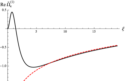
Figure 1: The evolution of $\Re\!\kern 0.83328pt\mathfrak{e}\kern 0.83328pt\widetilde{\Omega}^{(1)}_{\epsilon}$ (continuous black line) and its asymptotic value (red dashed line).

Figure 2: The evolution of the expression that defines $\beta_{\epsilon}$ (the right-hand side of Eq. (77) without taking the limit) as a function of $\xi$.

The difficulty in solving this part lies in the presence of the logarithmic term both in the source (62) and the asymptotic limit (70). In fact, if one removes this term, it is possible to solve equation (73) and obtain the value of $\beta_{\epsilon}$ analytically. This analysis is presented in the Appendix, in order to show that the presence of the logarithmic term, even if it is divergent in both early-time ($\xi\rightarrow\infty$) and late-time ($\xi\rightarrow 0$) limits, does not change the result drastically.

The complete equation (73) must be solved by numerical methods. In order to impose the initial condition (70), one needs to choose an initial large value of $\xi=\xi_{\text{initial}}$ and insert that value into the function

$$\widetilde{\Omega}^{(1)}_{\epsilon}(\xi_{\text{initial}})=-\frac{1}{12}\left[23-6\ln\xi_{\text{initial}}\right].$$ (83)

Note that it is very convenient to pick up different values for $\xi_{\text{initial}}$ to check that the final result does not depend on it. In particular, we have chosen $\xi_{\text{initial}}=10^{6}$, $10^{7}$, and $10^{8}$. The absolute difference between the various $\Omega^{(1)}_{\epsilon}(\xi)$, as computed for those different values, is less than $10^{-6}$ during the whole evolution (for any of the considered values of $\xi$), which translates to a negligible difference of around $10^{-5}$ in the value of $\beta_{\epsilon}$. In fact, in Fig. 1 it is possible to see that $\Omega^{(1)}_{\epsilon}$ tends very quickly to its asymptotic value, which explains the very weak dependence of the numerical solution on the chosen value of $\xi_{\text{initial}}$.

Finally, in order to compute numerically $\beta_{\epsilon}$, we have evaluated the expression that appears in its definition (77) for a very small value of $\xi=10^{-3}$, which leads to

$$\beta_{\epsilon}\approx-1.98.$$ (84)

Note that all the different $\Omega$ tend to vanish as $\xi\rightarrow 0$ and thus one cannot numerically compute the limit (77) by evaluating it at $\xi=0$. Nonetheless, in Fig. 2 the evolution of the right-hand side of (77) (without the limit taken) has been plotted, in order to show that the limit behaves smoothly and is well defined.

VI.5 The $\gamma$ part

Equation (74) for $\widetilde{\Omega}^{(1)}_{\gamma}$ is the most intricate one. It is, in particular, coupled to the equation for $\widetilde{\Omega}^{(1)}_{\text{dS}}$. As in the previous subsection, for the computation of $\beta_{\epsilon}$, there seems to be no way to write the solution analytically in terms of special functions and thus, it is necessary to resort to a numerical resolution. Nevertheless, the presence of the sine and cosine integral functions in the source term (63) makes it computationally highly demanding to deal with this equation numerically for large values of their argument. Thus, at early times ($\xi\gg 1$), it will be very convenient to consider instead their series expansion.

Therefore, we have applied the following procedure. First, these two functions are replaced by their series expansion in inverse powers of $\xi$ up to 20th order in the source term (63). Then, equation (74) is solved with this approximated source term and by imposing the initial data $\widetilde{\Omega}^{(1)}_{\gamma}=3/8$ for a very large initial time $\xi=\xi_{\text{initial}}\gg 1$. Next, the obtained numerical solution is used as initial data at a still large, but smaller value, of $\xi=\xi_{\text{intermediate}}<\xi_{\text{initial}}$, for Eq. (74) with the full form of its source term (63). Finally, this latter equation is solved and, with this numerical solution at hand, one can compute the expression on the left-hand side of Eq. (78), whose limit as $\xi\rightarrow 0$ will define our quantity of interest $\beta_{\gamma}$. As in the previous subsection, this limit is numerically computed by evaluating the corresponding expression for a small value of $\xi$.

In order to check the robustness of this method, different values for $\xi_{\text{initial}}$ and $\xi_{\text{intermediate}}$ have been used. In particular, we have chosen $\xi_{\text{initial}}$ as $10^{8}$, $10^{9}$, and $10^{10}$, while for $\xi_{\text{intermediate}}$ the values 100, 400, and 800 have been picked up. We find that the largest absolute difference between $\Re\!\kern 0.83328pt\mathfrak{e}\kern 0.83328pt\widetilde{\Omega}^{(1)}_{\gamma}$, as computed with the solution corresponding to these different values, during the whole evolution turns out to be smaller than $10^{-4}$. This is translated to an absolute difference of a similar order for $\beta_{\gamma}$. In fact, a value of $\beta_{\gamma}\approx 2.56$ is found and, thus, the error due to assuming an approximate equation for early times is very small.

The evolution of the real part of $\widetilde{\Omega}^{(1)}_{\gamma}$ is shown in Fig. 3, in combination with its asymptotic value $3/8$. Note that $\widetilde{\Omega}^{(1)}_{\gamma}(\xi)$ is a non-oscillating solution and approaches its asymptote from below very quickly. In Fig. 4, the evolution of the relation that defines $\beta_{\gamma}$ [the right-hand side of relation (78) without taking the limit] is shown in terms of $\xi$. As can be seen clearly in the figure, its late-time limit behaves smoothly and leads to the value

$$\beta_{\gamma}\approx 2.56.$$ (85)

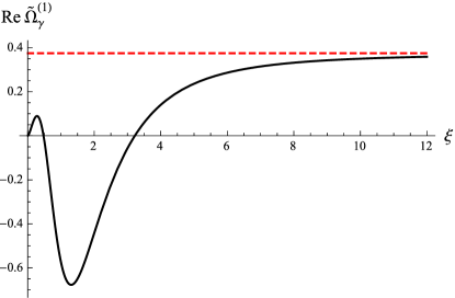
Figure 3: The evolution of $\Re\!\kern 0.83328pt\mathfrak{e}\kern 0.83328pt\widetilde{\Omega}^{(1)}_{\gamma}$ (black continuous line) and its asymptotic value 3/8 (red dashed line).

Figure 4: The evolution of the expression that defines $\beta_{\gamma}$ (the right-hand side of Eq. (78) without taking the limit) as a function of $\xi$.

VII Results and observability

In this section we will summarize our results and obtain the explicit form of the different parameters of the power spectrum, in particular the spectral indices and their running. We will also comment on the magnitude of the obtained corrections and the possibility of observing them. Finally, we will give the form of the correction for the $C_{\ell}$ coefficients used in the CMB data analysis.

VII.1 Parameters of the power spectra

The main results of this paper are the corrected forms of the power spectra for gauge-invariant scalar and tensor modes:

$${\cal P}_{\text{S}}^{(1)}(k) = {\cal P}_{\text{S}}^{(0)}(k)\Big{\{}1+\Delta_{\text{S}}\Big{\}}\,,$$ (86)

$${\cal P}_{\text{T}}^{(1)}(k) = {\cal P}_{\text{T}}^{(0)}(k)\Big{\{}1+\Delta_{\text{T}}\Big{\}}\,,$$ (87)

where ${\cal P}_{\text{S}}^{(0)}(k)$ and ${\cal P}_{\text{T}}^{(0)}(k)$ are the usual power spectra, which can be obtained in the approximation of quantum fields propagating on fixed cosmological backgrounds and which are explicitly given in (53) and (54), respectively. These correspond to the standard result derived usually by other means (see e.g. PU09 ). The quantum-gravity corrections are thus encoded in the $\Delta_{\text{S}}$ (75) and $\Delta_{\text{T}}$ (79) terms, with the $\beta_{\text{dS}}$, $\beta_{\epsilon}$ and $\beta_{\gamma}$ computed, respectively, in (82), (84), and (85). Inserting explicitly these numerical values and replacing the auxiliary parameter $\gamma$ defined in (39) by $\epsilon$ and $\delta$, the corrections to the power spectra read as follows:

$$\Delta_{\text{S}} = \frac{H_{k}^{2}}{m_{\text{P}}^{2}}\left(\frac{\bar{k}}{k}\right)^{3}\bigl{(}0.988+3.14\,\epsilon-2.56\,\delta\bigr{)}\,,$$ (88)

$$\Delta_{\text{T}} = \frac{H_{k}^{2}}{m_{\text{P}}^{2}}\left(\frac{\bar{k}}{k}\right)^{3}\bigl{(}0.988+0.58\,\epsilon\bigr{)}\,.$$ (89)

Here, we have reverted the rescaling applied in (6) and a reference wave number $\bar{k}=1/\mathfrak{L}$ has been defined as the inverse of the length scale introduced to regularize the spatial integral.

Since the dependence of the quantum-gravity corrections on the $k$ wave numbers have been analytically obtained, it is possible to derive the spectral indices and their runnings by direct computation. We will use the usual parametrization of the power spectra given by the following power-law relation,

$${\cal P}_{{\text{S}}}^{(1)}(k) = A_{{\text{S}}}\left(\frac{k}{k_{*}}\right)^{n_{\text{S}}-1+\alpha_{\text{S}}\ln(k/k_{*})},$$ (90)

$${\cal P}^{(1)}_{{\text{T}}}(k) = A_{{\text{T}}}\left(\frac{k}{k_{*}}\right)^{n_{\text{T}}+\alpha_{\text{T}}\ln(k/k_{*})},$$ (91)

where higher-order terms in $\ln(k/k_{*})$ have been neglected in the exponent and the pivot scale $k_{*}$ has been introduced. In this way, at a linear level in the slow-roll parameters, we obtain for the scalar sector

$$n_{\text{S}}-1:=\left.\frac{{\rm d}\ln{\cal P}_{\text{S}}^{(1)}(k)}{{\rm d}\ln k}\right|_{k=k_{*}}$$ (92)

$$=2\delta-4\epsilon-\frac{H_{k}^{2}}{m_{\text{P}}^{2}}\left(\frac{\bar{k}}{k_{*}}\right)^{3}\bigl{[}3\beta_{\text{dS}}+\epsilon(2\beta_{\text{dS}}+3\beta_{\epsilon}+6\beta_{\gamma})$$

$$\qquad\qquad\qquad\qquad\qquad\qquad\qquad\qquad\qquad\qquad-3\delta\beta_{\gamma}\bigr{]}$$

$$\approx 2\delta-4\epsilon-\frac{H_{k}^{2}}{m_{\text{P}}^{2}}\left(\frac{\bar{k}}{k_{*}}\right)^{3}\left(2.96+11.40\,\epsilon-7.68\,\delta\right),$$

with the first two terms taken together being the usual first-order approximation of the spectral index. In order to obtain this result, the relation

$$\frac{{\rm d}\ln H_{k}}{{\rm d}\ln k}=-\epsilon,$$ (93)

has been used. Similarly, for the tensor sector, one obtains

$$n_{\text{T}} := \left.\frac{{\rm d}\ln{\cal P}_{\text{T}}^{(1)}(k)}{{\rm d}\ln k}\right|_{k=k_{*}}$$

$$= -\,2\epsilon-\frac{H_{k}^{2}}{m_{\text{P}}^{2}}\left(\frac{\bar{k}}{k_{*}}\right)^{3}\left[3\beta_{\text{dS}}+\epsilon(3\beta_{\epsilon}+3\beta_{\gamma}+2\beta_{\text{dS}})\right]$$

$$\approx -\,2\epsilon-\frac{H_{k}^{2}}{m_{\text{P}}^{2}}\left(\frac{\bar{k}}{k_{*}}\right)^{3}\left(2.96+3.72\,\epsilon\right).$$

Finally, one can also obtain the running of the spectral indices,

$$\alpha_{\text{S}}:=\left.\frac{{\rm d}n_{\text{S}}}{{\rm d}\ln k}\right|_{k=k_{*}},$$ (95)

$$\alpha_{\text{T}}:=\left.\frac{{\rm d}n_{\text{T}}}{{\rm d}\ln k}\right|_{k=k_{*}},$$ (96)

by taking into account the dependence of the slow-roll parameters on the wave number. In particular, up to second-order terms we have

$$\frac{{\rm d}\epsilon}{{\rm d}\ln k} = 2\epsilon(\epsilon-\delta),$$ (97)

$$\frac{{\rm d}\delta}{{\rm d}\ln k} = 2\epsilon(\epsilon-\delta)-\theta,$$ (98)

where the second-order slow-roll parameter $\theta$ is defined as

$$\theta:=\frac{\dot{\epsilon}-\dot{\delta}}{H}.$$ (99)

In this way, one gets by direct computation the results

$$\alpha_{\text{S}} = 4\epsilon(\delta-\epsilon)-2\theta$$

$$\!\!+\,\frac{3H_{k}^{2}}{m_{\text{P}}^{2}}\left(\frac{\bar{k}}{k_{*}}\right)^{3}\!\bigl{[}3\beta_{\text{dS}}+\epsilon(4\beta_{\text{dS}}+3\beta_{\epsilon}+6\beta_{\gamma})-3\delta\beta_{\gamma}\bigr{]}$$

$$\approx 4\epsilon(\delta-\epsilon)-2\theta$$

$$\!\!+\,\frac{H_{k}^{2}}{m_{\text{P}}^{2}}\left(\frac{\bar{k}}{k_{*}}\right)^{3}\left(8.89+40.12\,\epsilon-23.04\,\delta\right),$$

$$\alpha_{\text{T}} = 4\epsilon(\delta-\epsilon)$$

$$\!\!+\,\frac{3H_{k}^{2}}{m_{\text{P}}^{2}}\left(\frac{\bar{k}}{k_{*}}\right)^{3}\Bigl{[}3\beta_{\text{dS}}+\epsilon(4\beta_{\text{dS}}+3\bigl{(}\beta_{\epsilon}+\beta_{\gamma})\bigr{)}\Bigr{]}$$

$$\approx 4\epsilon(\delta-\epsilon)+\,\frac{H_{k}^{2}}{m_{\text{P}}^{2}}\left(\frac{\bar{k}}{k_{*}}\right)^{3}\left(8.89+17.08\,\epsilon\right),$$

where only the first-order slow-roll terms have been kept in the correction term. Note that the prefactors in the correction term for the runnings get larger than for the spectral indices due to the fact that the usual parametrization (90)–(91) is not a good fit to the obtained quantum-gravity correction.

Let us finally also give the quantum-gravitational correction to the $r$-parameter (27). Since this correction is given by (80), we obtain

$$r^{(1)}\approx 16\epsilon\left(1+2.56\,\frac{H_{k}^{2}}{m_{\rm P}^{2}}\left(\frac{\bar{k}}{k}\right)^{3}(\delta-\epsilon)\right).$$ (102)

In most models $\delta-\epsilon=-\dot{\epsilon}/2H\epsilon<0$, thus the correction gives a small negative contribution to the scalar-to-tensor ratio. Note that, in the pure de Sitter case there is no correction for this quantity, so it arises entirely from the slow-roll part.

VII.2 Estimation of the magnitude of the correction

In order to give an estimation of the magnitude of the corrections for different quantities, one necessarily needs to assume a specific value for the scale $\bar{k}=1/\mathfrak{L}$. It seems reasonable to understand this scale as an infrared cut-off and relate it to the largest scale that could influence the CMB ($\bar{k}\approx 10^{-4}\,\text{Mpc}^{-1}$). Nonetheless, in the literature there are some analyses that try to fix its value by other means. In particular, in Ref. KTV16 , which is based on a similar semiclassical approach to the geometrodynamical quantization of the present problem, arbitrary parameters are considered in front of the correction factor $H_{k}^{2}\bar{k}^{3}/(m_{\rm P}^{2}k^{3})$ and they are fitted with the observational data from the Planck mission Planck . In particular, the best fit obtained relates $\bar{k}$ to the size of galaxies or galaxy clusters ($\bar{k}\approx 1\,\text{Mpc}^{-1}$). The meaning of such a scale is, however, not clear. All the above being said, in order to give an estimate of the magnitude of the correction we have obtained, here we will assume $\bar{k}$ to be equal to the pivot scale chosen by the Planck mission, that is $\bar{k}=k_{*}=0.05\,\text{Mpc}^{-1}$. At the end of this subsection, we will comment on the maximum possible value of $\bar{k}$ not to contradict the experimental data.

As we have shown in our previous work BKK , taking into account the energy scale of inflation in combination with the upper bound given by the Planck mission Planck for the scalar-to-tensor ratio $r\lesssim 0.11$, it is possible to derive the following condition,

$$\frac{H_{\text{inf}}}{m_{\rm P}}\lesssim 1.3\times 10^{-5}\,,$$ (103)

$H_{\text{inf}}$ being the average Hubble parameter during inflation. In the following, in order to give estimates for the correction to the quantities derived in the previous section, we will assume that $H_{k}=H_{\text{inf}}$.

In addition, the experimental constraint for the spectral index, $n_{\text{S}}\approx 0.968\pm 0.006$ (see Planck ), implies that $\epsilon\lesssim 0.007$ and $\delta\approx-0.002$. With these values at hand, we can give an estimate for the upper limits of the quantum-gravity correction for scalar and tensor perturbations as follows:

$$\left|\Delta_{\text{S}}\right| \lesssim 2\times 10^{-10},\,\quad\left|\Delta_{\text{T}}\right|\lesssim 2\times 10^{-10}.$$ (104)

Since the value of the slow-roll parameters is so small and the dominant de Sitter contribution $\beta_{\text{dS}}$ has a value close to 1, the approximated upper bounds for the corrections coincide with the approximated maximal value of the ratio $H_{k}^{2}/m_{\rm P}^{2}$. Using the estimated values for the slow-roll parameters, we can, however, deduce that the corrections for both kinds of perturbations differ by about $2\,\%$:

$$\frac{\Delta_{\text{S}}}{\Delta_{\text{T}}}\approx 1.02\,.$$ (105)

Inserting the estimated numbers for $\epsilon$ and $\delta$, we can immediately see that the correction to the spectral index is significantly smaller than the statistical uncertainty in the Planck data:

$$\left[n_{\text{S}}^{(1)}-n_{\text{S}}^{(0)}\right]_{k=\bar{k}}\approx-3.1\,\frac{H_{\text{inf}}^{2}}{m_{\text{P}}^{2}}\approx-5\times 10^{-10}\,.$$ (106)

In this case, the quantum-gravitational correction to the spectral index is also tiny,

$$\left[n_{\text{T}}^{(1)}-n_{\text{T}}^{(0)}\right]_{k=\bar{k}}\approx-3.0\,\frac{H_{0,\text{inf}}^{2}}{m_{\text{P}}^{2}}\approx-5\times 10^{-10}\,.$$ (107)

Estimating the magnitude of the quantum-gravity correction for the running gives

$$\left[\alpha_{\text{S}}^{(1)}-\alpha_{\text{S}}^{(0)}\right]_{k=\bar{k}} \approx 9.2\,\frac{H_{\text{inf}}^{2}}{m_{\text{P}}^{2}}\approx 2\times 10^{-9}\,,$$ (108)

$$\left[\alpha_{\text{T}}^{(1)}-\alpha_{\text{T}}^{(0)}\right]_{k=\bar{k}} \approx 9.0\,\frac{H_{\text{inf}}^{2}}{m_{\text{P}}^{2}}\approx 2\times 10^{-9}\,.$$ (109)

Finally, the upper bound for the correction of the scalar-to-tensor ratio can be estimated as

$$\left[\frac{r^{(1)}-r^{(0)}}{r^{(0)}}\right]_{k=\bar{k}}\approx-0.023\,\frac{H_{\text{inf}}^{2}}{m_{\text{P}}^{2}}\approx-4\times 10^{-12}\,.$$ (110)

As can be seen, all corrections are very small and they are inside the current experimental error bars.

Let us finally comment on the maximally allowed value for $\bar{k}$ by the experimental data. The fact that the experimental errors are larger than the corrections (88)–(89) we have obtained leads to the following relation,

$${\bar{k}}_{\rm max}=\left(\frac{m^{2}_{\rm P}\Delta_{\rm exp}}{H^{2}_{\rm inf}}\right)^{1/3}k_{*},$$ (111)

$\Delta_{\rm exp}$ being the relative experimental error in the power spectrum. In order to give a rough estimate, we assume that this error is of order one, which, as can be seen in HS15 , is a very high bound. Using the maximum value for the ratio $H_{\rm inf}/m_{\rm P}$ found in (103), we get

$${\bar{k}}_{\rm max}\approx 100\,{\rm Mpc}^{-1}.$$ (112)

This implies a minimum value for the length scale ${\mathfrak{L}}_{\rm min}\approx 10^{-2}\,{\rm Mpc}$. Note, even though, that a lower value of $H_{\rm inf}/m_{\rm P}$ would increase ${\bar{k}}_{\rm max}$.

VII.3 CMB temperature anisotropies

In this subsection we will obtain the correction for the CMB temperature anisotropies, which are usually expressed by the quantities $C_{\ell}$ as defined below. In order to obtain these coefficients, it is necessary to evolve the scalar power spectrum through subsequent phases of the universe from the end of inflation until today. In addition, one finally needs to project it on the celestial sphere. This whole procedure can be reduced to computing the following integral, which is usually done numerically,

$$C^{(i)}_{\ell}=\int_{0}^{\infty}\frac{\mathrm{d}k}{k}\,\mathcal{P}^{(i)}_{\text{S}}(k)\,\Theta_{\ell}^{2}(k),$$ (113)

with $i=0,1$ denoting the uncorrected and corrected coefficients, respectively, and $\Theta_{\ell}(k)$ being the transfer function. For large scales (small $\ell$), however, it is possible to solve this integral analytically. In this regime, the fluctuations were well outside the horizon at the end of recombination and thus they were not affected by subhorizon physics. Therefore, it is only necessary to take into account the primordial spectrum and perform the projection on the celestial sphere. In particular, the transfer function can in this case be given in terms of the spherical Bessel functions $j_{\ell}$ as follows Dodelson ,

$$\Theta_{\ell}(k)=\frac{1}{3}\,j_{\ell}(k[\eta_{\text{hor}}-\eta_{\text{rec}}]),$$ (114)

where $\eta_{\text{hor}}$ is the conformal time at horizon crossing and $\eta_{\text{rec}}$ the conformal time at recombination.

Let us define the quantum-gravitational correction to the temperature anisotropies in the following way,

$$\Delta C_{\ell}:=C_{\ell}^{(1)}-C_{\ell}^{(0)}.$$ (115)

Applying the results for the corrected scalar power spectrum, we get that, for large scales, this correction has the following form,

$$\Delta C_{\ell}\approx\frac{1}{4\pi^{2}}\int_{0}^{\infty}\frac{{\rm d}k}{k\,\epsilon}\left(\frac{H_{k}}{m_{\text{P}}}\right)^{4}\left(\frac{\bar{k}}{k}\right)^{3}\,j^{2}_{\ell}(k[\eta_{\text{hor}}-\eta_{\text{rec}}]),$$ (116)

The approximate symbol in this equation stands for two reasons. On the one hand, we are assuming an approximated transfer function. And, on the other hand, the overall factor that appears in the correction term (88), which depends on the slow-roll parameters but is of order one, has been dropped. At this point, as explained in Baumann , we use the fact that the Bessel function is strongly peaked around $k|\eta_{\text{hor}}-\eta_{\text{rec}}|\approx\ell$ and effectively acts as a Dirac delta mapping between $k$ and $\ell$. Therefore, one can integrate the explicit $k$ dependences in the last integral, which leads to

$$\Delta C_{\ell}\approx\!\!\frac{3}{4\pi\epsilon}\!\!\left(\!\frac{H_{k}}{m_{\text{P}}}\!\right)^{4}\!\!\!\!\frac{|\bar{k}(\eta_{\text{hor}}-\eta_{\text{rec}})|^{3}}{(2\ell-3)(2\ell-1)(2\ell+1)(2\ell+3)(2\ell+5)},$$ (117)

while the implicit $k$-dependences on $H_{k}$ and $\epsilon$ should be evaluated at $k|\eta_{\text{hor}}-\eta_{\text{rec}}|\approx\ell$. Applying exactly the same approximations, it is straightforward to obtain also the well-known result for the uncorrected temperature anisotropies at large scales:

$$C_{\ell}^{(0)}\approx\frac{1}{8\pi^{2}\epsilon}\left(\!\frac{H_{k}}{m_{\text{P}}}\!\right)^{2}\frac{1}{\ell(\ell+1)}\,,$$ (118)

which does not have any explicit dependence on $(\eta_{0}-\eta_{\rm rec})$ and, for a scale-invariant spectrum (constant $H_{k}$ and $\epsilon$) is just proportional to the inverse of $\ell(\ell+1)$.

Thus, due to a correction proportional to $k^{-3}$ in the power spectrum, the temperature anisotropies get a correction that goes as the inverse of a fifth-order polynomial in $\ell$ for large scales. However, since the uncorrected $C_{\ell}^{(0)}$ go with $\ell^{-2}$, the relative correction $\Delta C_{\ell}/C^{(0)}_{\ell}$ is of order $\ell^{-3}$. As commented in the previous section, especially due to the presence of $\bar{k}$ is this correction, it is difficult to be certain about its absolute value. We have thus plotted the behavior of the relative correction with respect to $\ell$ without the physical prefactors in Fig. 5.

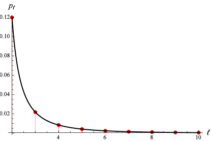
Figure 5: The ratio of the correction $\Delta C_{\ell}$ to the uncorrected $C_{\ell}^{(0)}$ without the non-numerical prefactors, such that we have
$p_{\ell}:=3\pi\,\ell(\ell+1)\left[(2\ell-3)(2\ell-1)(2\ell+1)(2\ell+3)(2\ell+5)\right]^{-1}$.

We can also check the relative values and see that the correction drops very quickly with $\ell$. For instance, comparing it for the first multipoles:

$$\frac{\Delta C_{\ell=3}}{\Delta C_{\ell=2}}\approx 0.09,\quad\frac{\Delta C_{\ell=4}}{\Delta C_{\ell=2}}\approx 0.02,\quad\frac{\Delta C_{\ell=5}}{\Delta C_{\ell=2}}\approx 0.007.$$

It is important to note that the qualitative behavior derived in this section for correction of the temperature anisotropies essentially comes from the explicit $k^{-3}$ dependence of the correction of the power spectrum, which has been obtained in several approaches (see, for instance, KTV16 ).

We can also give an estimate of how large the Hubble parameter, i.e. the energy scale, during inflation would have to be such that one could see a correction of our type. Given that cosmic variance behaves like

$$\frac{\Delta C_{\ell}^{{}^{\text{CV}}}}{C_{\ell}^{(0)}}=\sqrt{\frac{2}{2\ell+1}},$$ (119)

one can conclude that for $\ell=2$, where cosmic variance is about $\Delta C_{2}^{{}^{\text{CV}}}/C_{2}^{(0)}\approx 0.63$ and our quantum-gravitational correction is given by

$$\frac{\Delta C_{2}}{C_{2}^{(0)}}\approx 0.12\,\left(\!\frac{H_{k}}{m_{\text{P}}}\!\right)^{2}\,|\bar{k}(\eta_{\text{hor}}-\eta_{\text{rec}})|^{3},$$ (120)

the remaining factors in the above expression would have to be larger than 5 in order to clearly see an effect in the CMB data. Using $\bar{k}=0.05\,\text{Mpc}^{-1}$, and given that $|\eta_{\text{hor}}-\eta_{\text{rec}}|$ can be estimated to be about $700\,\text{Mpc}$ (see e.g. Tab. I in AG16 ), the factor $|\bar{k}(\eta_{\text{hor}}-\eta_{\text{rec}})|^{3}$ turns out to be of order $5\times 10^{4}$. Therefore, in order to see an effect, $(H_{k}/m_{\text{P}})\gtrsim 10^{-2}$ would be required, which is by far outside the range (103) allowed by the measured tensor-to-scalar ratio. Moreover, if we use the maximum allowed value by the latter limit for the Hubble factor, it would be necessary for $\bar{k}$ to be around $\bar{k}\approx 5\,\text{Mpc}^{-1}$ to get an observable effect. This value is significantly smaller than the maximum value ${\bar{k}}_{\rm max}$ derived in (112).

VIII Conclusions

In this paper quantum-gravitational corrections for the power spectra of the gauge-invariant scalar and tensor perturbations have been obtained in the slow-roll regime. In particular, the corrected form for the scalar and tensor power spectrum is given, respectively, by (23) and (25), where $\Delta_{\text{S}}$ is given in (75) and $\Delta_{\text{T}}$ in (79) in terms of the numerical coefficients $\beta_{\text{dS}}$, $\beta_{\epsilon}$ and $\beta_{\gamma}$. These coefficients have been computed by solving the linearized evolution equation for the Gaussian width $\Omega^{(1)}$ with natural initial data (in the sense that the initial state, which is constructed as a small deformation of the usual Bunch-Davies vacuum, best describes in this context the expected properties of a freely evolving mode). Their values are given in (82), (84), and (85), respectively.

The above results generalize the results for the de Sitter case obtained earlier in BKK to a more realistic scenario of slow-roll inflation. In particular, and as one would naively expect, the main part of the correction is due to the de Sitter contribution (which introduces an enhancement of the spectrum), whereas the slow-roll part slightly modifies it. Let us at this point briefly comment on the results of KTV16 , obtained from an alternative expansion of the Wheeler-DeWitt equation. As in our treatment, the authors find quantum-gravitational correction terms proportional to $H_{\text{inf}}^{2}/(m_{\rm P}^{2}k^{3})$. Nonetheless, their result for the slow-roll approximation is not just a small perturbation of the de Sitter case, but can give a comparable contribution for large scales, which can even lead to a power loss instead of an enhancement of the power spectra.

Moreover, let us stress that the kind of correction that has been obtained in this analysis – being proportional to the factor $H_{\text{inf}}^{2}\bar{k}^{3}/(m_{\rm P}^{2}k^{3})$ – has appeared in several different approaches in the context of quantum geometrodynamics Sasha1 ; Sasha2 ; Sasha3 ; KTV16 . The form of this correction is not completely unexpected. In fact, it is possible to argue, already on dimensional grounds, that $(H_{\text{inf}}/m_{\rm P})^{2}$ is the only non-dimensional parameter that one could use to include perturbatively (as a power series expansion) quantum-gravity corrections. Furthermore since, due to the background homogeneity, one needs to introduce explicitly a volume (${\mathfrak{L}}^{3}=1/\bar{k}^{3}$) in order to regularize the spatial integral in the action, another dimensionless quantity $(\bar{k}/k)^{3}$ enters the game. Nevertheless, in principle, the power of this latter quantity might have been different and thus it is very interesting to see how the same correction is explicitly realized in different specific models.

In the last section we have also analyzed the magnitude of the obtained corrections and the possibility of observing them experimentally. The most difficult issue in order to give a precise estimation is that, due to the regularization of the spatial integral in the action, a length scale needs to be considered. The power spectrum then depends on that length scale and there seems to be nothing physical to fix it. As we have commented, in the main part of the paper, the most reasonable choice is to take it as an infrared cut-off, relating it to the largest observable scale in the CMB. In our case, just to give an approximated estimate, we have chosen it as the length scale of a typical mode that affects the CMB. In particular we have chosen the pivot scale selected by the Planck mission. In this way, we have obtained that the corrections for all different parameters of the power spectra (spectral indices and runnings) are well inside the current experimental error bars.

Finally, we have also obtained the qualitative form of the correction induced in the CMB temperature anisotropies by this quantum-gravity effect. The analysis we have performed is valid for large scales (small $\ell$), for which quantum-gravity effects are expected to be more relevant. In particular, it shows that a correction of the form $k^{-3}$ which, as commented above, seems very generic in this context, leads to a relative correction of the order $\ell^{-3}$ for the anisotropies, which thus quickly declines with increasing $\ell$.

With this paper we conclude our investigations on quantum-gravitational corrections arising from a canonical quantization of a perturbed universe model using the Wheeler-DeWitt equation. The effects on large scales we have obtained are, for a reasonable choice of $\bar{k}$, not observable in the CMB data and since we have used a generic slow-roll model that encompasses a wide range of inflationary models, using more refined models that obey the slow-roll approximation would not enhance the corrections. Nonetheless, it is still an open question whether such corrections can be observed in situations where cosmic variance is not present; for example, in galaxy-galaxy correlation functions.

Appendix A Computation of $\beta_{\epsilon}$ removing the divergent logarithmic term

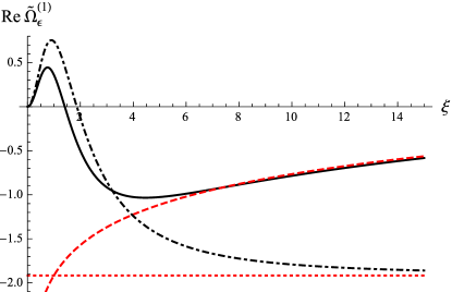
Figure 6: The evolution of the real part of $\widetilde{\Omega}^{(1)}_{\epsilon}$ is shown, for different ranges of values of $\xi$, as given by its full equation (black continuous line) and as obtained by dropping the logarithmic term (black dashed-dotted line). Their corresponding asymptotes are shown as a red-dashed line and as a red-dotted line, respectively.

In this Appendix, Eq. (73), with the logarithmic term dropped, will be solved in order to show that, even if this term is divergent in both late and early time limits, the value that is obtained for $\beta_{\epsilon}$ does not change dramatically. Note that, if one removes the logarithmic term from the source term (62), one should also remove it from the initial condition (70).

Interestingly, in this case Eq. (73) can be analytically solved, and the solution takes the following form:

$$\widetilde{\Omega}^{(1)}_{\epsilon}=\; \frac{1}{12}\,\mathrm{e}^{2}\xi^{2}\left(\xi^{2}+1\right)^{2}\Big{[}3\,\mathrm{e}^{2{\rm i}\xi}(\xi+\mathrm{i})^{2}(-4\mathrm{e}^{2}C$$

$$+33\,\Gamma(0,2\mathrm{i}\xi-2)+11\,\mathrm{e}^{4}\Gamma(0,2\mathrm{i}\xi+2))$$

$$-\mathrm{e}^{2}\left(12\left(\xi^{2}+1\right)+11\,(1+\xi(\xi-6\mathrm{i}))\right)\Big{]},$$ (121)

where $C$ is an integration constant. If we analyze the behavior of this solution at $\xi\rightarrow\infty$, we find that

$$\widetilde{\Omega}^{(1)}_{\epsilon}\approx-\frac{23}{12}-C\,\mathrm{e}^{2\mathrm{i}\xi}.$$ (122)

Therefore, in order to have a non-oscillating solution, we choose $C=0$.

Finally, we compute the limit defined in Eq. (77) and find the following value of $\beta_{\epsilon}$:

$$\beta_{\epsilon}=1+\frac{11}{12\,\mathrm{e}^{2}}(\mathrm{e}^{2}-3\,\mathrm{e}^{4}\text{Ei}(-2)-9\,\text{Ei}(2))\approx-2.62.$$ (123)

As commented above, this proves that the logarithmic term is indeed important to compute the precise value for $\beta_{\epsilon}$, but it is not critical in the sense that qualitatively the same result is obtained if one drops it.

In Fig. 6, the evolution of the real part of $\widetilde{\Omega}^{(1)}_{\epsilon}$ is shown for both the solution with and without the logarithmic term, in combination with their corresponding asymptotes. It can be seen that the tendency at late times is quite similar for both, which explains the weak dependence of $\beta_{\epsilon}$ on the commented term.

References

- (1) C. Kiefer, Quantum Gravity, International Series of Monographs on Physics 155, third edition (Oxford University Press, Oxford, 2012).
- (2) C. Kiefer and M. Krämer, Int. J. Mod. Phys. D 21, 1241001 (2012).
- (3) C. Kiefer and M. Krämer, Phys. Rev. Lett. 108, 021301 (2012).
- (4) D. Bini, G. Esposito, C. Kiefer, M. Krämer, and F. Pessina, Phys. Rev. D 87, 104008 (2013).
- (5) G. Calcagni, Ann. Phys. (Berlin) 525, 323 (2013); Erratum ibid. A165.
- (6) D. Bini and G. Esposito, Phys. Rev. D 89, 084032 (2014).
- (7) G. L. Alberghi, R. Casadio, and A. Tronconi, Phys. Rev. D 74, 103501 (2006).
- (8) A. Y. Kamenshchik, A. Tronconi, and G. Venturi, Phys. Lett. B 726, 518 (2013).
- (9) A. Y. Kamenshchik, A. Tronconi, and G. Venturi, Phys. Lett. B 734, 72 (2014).
- (10) A. Y. Kamenshchik, A. Tronconi, and G. Venturi, J. Cosmol. Astropart. Phys. 04 (2015) 046.
- (11) A. Y. Kamenshchik, A. Tronconi, and G. Venturi, Phys. Rev. D 94, 123524 (2016).
- (12) I. Agullo, A. Ashtekar, and W. Nelson, Phys. Rev. Lett. 109, 251301 (2012); Phys. Rev. D 87, 043507 (2013); Class. Quant. Grav. 30, 085014 (2013).
- (13) D. Martín de Blas and J. Olmedo, JCAP 06, 029 (2016).
- (14) B. Bolliet, J. Grain, C. Stahl, L. Linsefors, and A. Barrau, Phys. Rev. D 91, 084035 (2015).
- (15) S. Schander, A. Barrau, B. Bolliet, L. Linsefors, J. Mielczarek, and J. Grain, Phys. Rev. D 93 023531 (2016).
- (16) A. Ashtekar and B. Gupt, Class. Quantum Grav. 34, 014002 (2017).
- (17) C. Kiefer and T. P. Singh, Phys. Rev. D 44, 1067 (1991); C. Kiefer, Lect. Notes Phys. 434, 170 (1994).
- (18) C. Bertoni, F. Finelli, and G. Venturi, Class. Quantum Grav. 13, 2375 (1996).
- (19) D. Brizuela, C. Kiefer and M. Krämer, Phys. Rev. D 93, 104035 (2016).
- (20) V. F. Mukhanov, H. A. Feldman, and R. H. Brandenberger, Phys. Rep. 215, 203 (1992).
- (21) P. Peter and J.-P. Uzan, Primordial Cosmology (Oxford University Press, Oxford, 2009).
- (22) L. Parker and D. Toms, Quantum field theory in curved spacetime, Cambridge University Press, Cambridge, (2009).
- (23) J. Martin, V. Vennin, and P. Peter, Phys. Rev. D 86, 103524 (2012).
- (24) C. Kiefer, in: New Frontiers in Gravitation, edited by G. A. Sardanashvily and R. Santilli (Hadronic Press, Palm Harbor, 1995), p. 203; arXiv:gr-qc/9501001.
- (25) B. J. Broy, Phys. Rev. D 94, 103508 (2016).
- (26) P. A. R. Ade et al. (Planck Collaboration), Astron. Astrophys. 594, A13 (2016).
- (27) P. Hunt and S. Sarkar, JCAP 12, 052 (2015).
- (28) S. Dodelson, Modern Cosmology (Academic Press, Elsevier, 2003).
- (29) D. Baumann, Physics of the Large and the Small, TASI 09, Proceedings of the Theoretical Advanced Study Institute in Elementary Particle Physics, World Scientific (2009).