Coarse mesh partitioning for tree based AMR

Abstract

In tree based adaptive mesh refinement, elements are partitioned between processes using a space filling curve. The curve establishes an ordering between all elements that derive from the same root element, the tree. When representing more complex geometries by patching together several trees, the roots of these trees form an unstructured coarse mesh. We present an algorithm to partition the elements of the coarse mesh such that (a) the fine mesh can be load-balanced to equal element counts per process regardless of the element-to-tree map and (b) each process that holds fine mesh elements has access to the meta data of all relevant trees. As an additional feature, the algorithm partitions the meta data of relevant ghost (halo) trees as well. We develop in detail how each process computes the communication pattern for the partition routine without handshaking and with minimal data movement. We demonstrate the scalability of this approach on up to 917e3 MPI ranks and .37e12 coarse mesh elements, measuring run times of one second or less.

Keywords. Adaptive mesh refinement, coarse mesh, mesh partitioning, parallel algorithms, forest of octrees, high performance computing

AMS subject classification. 65M50, 68W10, 65Y05, 65D18

1 Introduction

Adaptive mesh refinement (AMR) has a long tradition in numerical mathematics. Over the years, the technique has evolved from a pure concept to a practical method, where the transition may be located somewhere in the mid-80s; see, for example, [5]. A second transition from serial to parallel computing, eventually parallelizing the storage of the mesh itself, has occured around the turn of the millennium (see e.g. [20]). Different flavors of the approach have been studied, varying in the shape of the mesh elements used (triangles, tetrahedra, quadrilaterals, cubes) and in the logical grouping of the elements.

Elements may actually not be grouped at all and assembled into an unstructured mesh, some recent references being [27, 46, 31]. The connectivity of elements can be modeled as a graph, and the partitioning of elements between parallel processes can be translated into partitioning the graph. Finding an approximate solution to this problem has been the subject of extensive research, some of which has lead to the development of software libraries [23, 17, 15]. In practice, the graph approach is often augmented by diffusive migration of elements. All in all, partitioning times of roughly 1e3 to 1e4 elements per second have been measured [13, 39, 16]. We may thus think of approaching the partitioning problem differently, trading the generality of the graph for a mathematical structure that offers rates of maybe 1e5 to 1e6 elements per second.

When we group elements by their size $h$, a particularly strict ansatz is the hierarchical, $h=2^{-\ell}$, using some refinement level $\ell\in\mathbb{Z}$. For square/cubic elements, we may introduce a rectangular grid of equal-sized ones and reduce the assembly of the mesh to the question of arranging such grids relative to each other. Block-structured methods do just that in varying instances of generality, some allowing free rotation and overlapping of blocks of any level [38], others imposing strict rules of assembly (such as not allowing rotation, but only shifts in multiples of $h$ [4]). Another such rule interprets elements as nodes of a tree, where the level $\ell$ takes on a second meaning as the depth of a node below the root [32].

Tree-based AMR can be implemented for any shape of element, where special 2D solutions exist [25] as well as the popular rectangles (2D) and cubes (3D) approach. The tree root is identified with the largest possible element and thus inherits its shape as a volume in space. This points directly at a practical limitation: how to represent domain geometries that have more complex shapes? One answer is to consider multiple tree roots and arrange them in the fashion of unstructured AMR, giving rise to a forest of elements [40, 41, 3]. The mesh of trees is sometimes called the coarse mesh, which is created a priori to map the topology and geometry of the domain with sufficient fidelity. Elements may then be refined and coarsened recursively, changing the mesh below the root of each tree.

Many simulations require one tree only, and the concept of the forest is not called upon. Popular forest AMR codes respect this fact by operating with no or minimal overhead in the special case of a one-tree forest. When multiple trees are needed, their number is limited by the available memory of contemporary computers to roughly a million per process [12]. While this number allows to execute most coarse meshing tasks in serial, we may still ask how to work with coarse meshes of say a billion or more trees total, such numbers being common in industrial and medical unstructured meshing. In this case, the coarse mesh needs to be partitioned between the processes, either by means of file I/O [7] or in-core, as we will discuss in this paper.

Most tree-based AMR codes make use of a space filling curve to order the elements within a tree [21, 43, 42] as well as points or other primitives [30]. Two main approaches for partitioning a forest of elements have been discussed [47], namely (a) assigning each tree and thus all of its elements to one owner process [34, 8] or (b) allowing a tree to contain elements belonging to multiple processes [3, 12]. The first approach offers a simpler logic, but may not provide acceptable load balance when the number of elements differs vastly between trees. The second allows for perfect partitioning of elements by number (the local numbers of elements between processes differ by at most one), but presents the issue of trees that are shared between multiple processes.

We choose paradigm (b) for speed and scalability, challenging us to solve an $n$-to-$m$ communication problem for every coarse mesh element. The objective of this paper is thus to develop how to do this without handshaking (i.e., without having to determine separately which process receives from which), and with a minimal number of senders, receivers, and messages. One corner stone is to avoid identifying a single owner process for each tree, but rather to treat all its sharer processes as algorithmically active under the premise that they produce a disjoint union of the information necessary to be transferred. In particular, each process shall store the relevant tree meta data to be readily available, eliminating the need to transfer this data from a single owner process.

In this paper, we also integrate the parallel transfer of ghost trees. The reason is that each process will eventually collect ghost elements, i.e., remote elements adjacent to its own. Although we do not discuss such an algorithm here, we note that ghost elements of any process may be part of trees that are not in its local set. To disconnect the ghost algorithm from identifying and transfering ghost trees, we perform this as part of the coarse mesh partitioning, presently across tree faces. We study in detail what information we must maintain to reference neighbor trees of ghost trees (that may themselves be either local, ghost, or neither) and propose an algorithm with minimal communication effort.

We have implemented the coarse mesh partitioning for triangles and tetrahedra using the SFC designed in [11], and for quadrilaterals and cubes exploiting the logic from [12]. To demonstrate that our algorithms are safe to use, we verify that (a) small numbers of trees require run times on the order of milliseconds and thus present no noticeable overhead compared to a serial coarse mesh, and that (b) the coarse mesh partitioning adds only a fraction of run time compared to the partitioning of the forest elements, even for extraordinarily large numbers of trees. We show a practical example of 3D dynamic AMR on 8e3 cores using 383e6 trees and up to 25e9 elements. To investigate the ultimate limit of our algorithms, we partition coarse meshes of up to .37e12 trees on a Blue Gene/Q system using 458e3 cores, obtaining a total run time of about 1s, a rate of 7e5 trees per second.

We may summarize our results by saying that partitioning the trees can be made no less costly than partitioning the elements, and often executes so fast that it does not make a difference at all. This allows a forest code that partitions both trees and elements dynamically to treat the whole continuum of forest mesh scenarios, from one tree with nearly trillions of elements on the one extreme to billions of trees that are not refined at all on the other, with comparable efficiency.

2 Forest based AMR

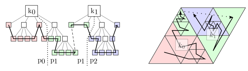
Figure 3: We patch multiple trees together to model complex geometries. Here, we show two trees $k_{0}$ and $k_{1}$ with an adaptive refinement. To store the forest mesh, we use a space-filling curve within each tree and the a-priori tree order between trees. On the left-hand side of the figure the refinement tree and its linear storage are shown. When we partition the forest mesh to $P$ processes (here, $P=3$), we cut the SFC in $P$ equal-size parts and assign part $i$ to process $i$.

We understand the connectivity of a forest as a mesh of root elements, which is effectively the coarsest possible mesh. We will simply call it coarse mesh in the following. Each root element may be subdivided recursively into elements, replacing one element by four (triangles and quadrilaterals) or eight (tetrahedra and cubes). For our purposes, the subdivision may be chosen freely by an application. Thus, in our context an element has two roles: one geometric as a volume in space and one logical as node of a tree. The leaf elements of the forest compose the forest mesh used for computation, see also Figures 1 and 3. The (leaf) elements may be used in a classical finite element/finite volume/dG setting or as a meta structure, for example to manage a subgrid in each leaf element [18, 33, 10, 24].

The order of elements is established first by tree and then by their index with respect to a space filling curve (SFC, see also [2]):

We enumerate the $K$ trees of the coarse mesh by $0,\dots,{K-1}$ and call the number $k$ of a tree its global index. With the global index we naturally extend the SFC order of the leaves: Let a leaf element of the tree k have SFC index $I$ (within that tree), then we define the combined index $(k,I)$. This index compares to a second index $(k^{\prime},J)$ as

$$(k,I)<(k^{\prime},J)\quad:\Leftrightarrow\quad\text{$k<k^{\prime}$ or ($k=k^{\prime}$ and $I<J$)}.$$ (1)

In practice we store the mesh elements local to a process in one contiguous array per locally non-empty tree in precisely this order.

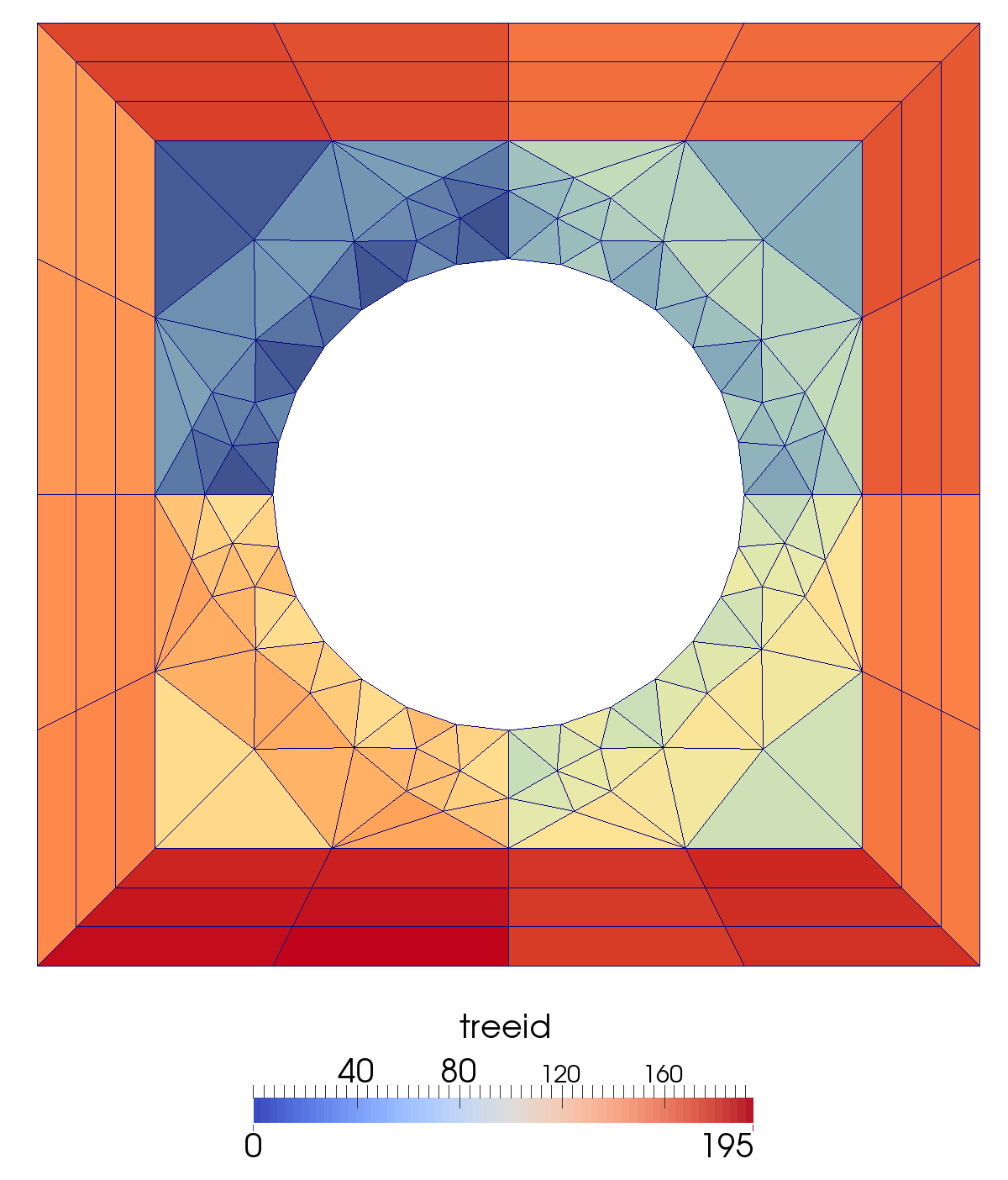
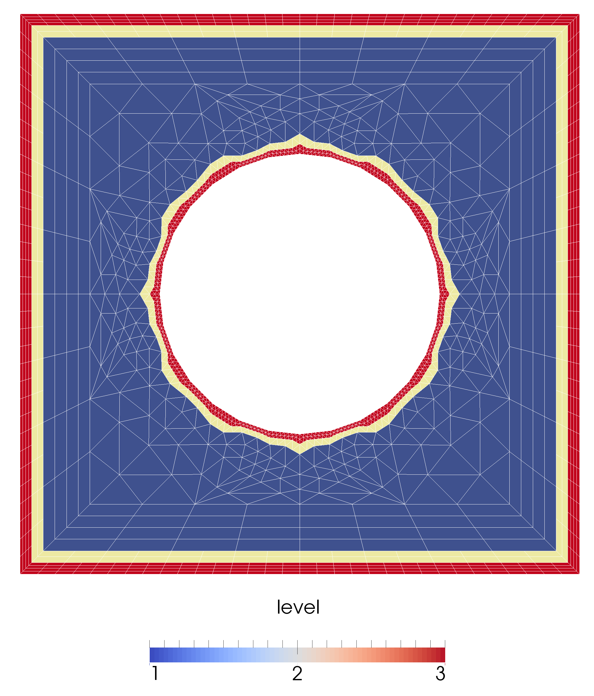
Figure 1: A mesh consists of two structures, the coarse mesh (left) that represents the connectivity of the domain, and the forest mesh (right) that consists of the leaf elements of a refinement and is used for computation. In this example the domain is a unit square with a circular hole. The color coding in the coarse mesh displays each tree’s unique and consecutive identifier, while the color coding in the forest mesh represents the refinement level of each element. In this example we choose an initial global level 1 refinement and a refinement of up to level 3 along the domain boundary.

2.1 The tree types and their connectivity

The trees of the coarse mesh can be of arbitrary type as long as they are all of the same dimension and fit together along their faces. In particular, we identify the following tree types:

• Points in 0D.

• Lines in 1D.

• Squares and triangles in 2D.

• Cubes and tetrahedra in 3D.

• Prisms and pyramids in 3D.

Coarse meshes consisting solely of prisms or pyramids are quite uncommon; these tree types are used primarily to transition between cubes and tetrahedra in hybrid meshes. The choice of SFC affects the ordering of the leaves in the forest mesh and thus the parallel partition of elements. Possibilities include, but are not limited to, the Hilbert, Peano, or Morton curves for cubes and squares [28, 37, 22, 44] as well as the Sierpiński or tetrahedral Morton curves for tetrahedra and triangles [1, 11]. In the t8code software used for the demonstrations in this paper we have so far implemented Morton SFCs for cubes and squares via the p4est library [9] and the tetrahedral Morton SFC for tetrahedra and triangles; other schemes may be added in a modular fashion.

2.2 Encoding of face-neighbors

The connectivity information of a coarse mesh includes the neighbor relation between adjacent trees. Two trees are considered neighbors if they share at least one lower dimensional face (vertex, face, or edge). Since all of this connectivity information can be concluded from codimension-1 neighbors, we restrict ourselves to those, denoting them uniformly by face-neighbors. At this point we do not consider neighbor relations across lower dimensional tree faces, as we believe without loss of generality for the partitioning algorithms to follow.

An application often requires a quick mechanism to access the face-neighbors of a given forest mesh element. If this neighbor element is a member of the same tree the computation can be carried out via the SFC logic, which involves only few bitwise operations for the cubical and tetrahedral Morton curves [26, 42, 12, 11]. If, however, the neighbor element belongs to a different tree, we need to identify this tree, given the parent tree of the original element and the tree face at which we look for the neighbor element. It is thus advantageous to store the face-neighbors of each tree in an array that is ordered by the tree’s faces. To this end, we fix the enumeration of faces and vertices relative to each other as depicted in Figure 2.

Figure 2: The vertex and face labels of the 2D (left) and 3D (right) tree types.

2.3 Orientation between neighbors

In addition to the global index of the neighbor tree across a face, we describe how the faces of the tree and its neighbor are rotated relative to each other. We allow all connectivities that can be embedded in a compact 3-manifold in such a way that each tree has positive volume. This includes the Moebius strip and Klein’s bottle and also quite exotic meshes, e.g. a cube whose one face connects to another in some rotation. We obtain two possible orientations of a line-to-line connection, three for a triangle-to-triangle- and four for a square-to-square connection.

We would like to encode the orientation of a face connection analogously to the way it is handled in p4est: At first, given a face $f$, its vertices are a subset of the vertices of the whole tree. If we order them accordingly and re-numerate them consecutively starting from zero, we obtain a new number for each vertex that depends on the face $f$. We call it the face corner number. If now two faces $f$ and $f^{\prime}$ meet, the corner $0$ of the face with the smaller face number is identified with a face corner $k$ in the other face. In p4est this $k$ is defined to be the orientation of the face connection.

In order for this operation to be well-defined, it must not depend on the choice of the first face when the two face numbers are the same, which is easily verified for a single tree type. When two trees of different types meet, we generalize to determine which face is the first one.

Definition 1.

We impose a semiorder on the 3-dimensional tree types as follows:

$$\begin{gathered}\lx@xy@svg{\hbox{\raise 0.0pt\hbox{\kern 31.41847pt\hbox{\ignorespaces\ignorespaces\ignorespaces\hbox{\vtop{\kern 0.0pt\offinterlineskip\halign{\entry@#!@&&\entry@@#!@\cr&\\&&\\&\crcr}}}\ignorespaces{\hbox{\kern-31.02202pt\raise 0.0pt\hbox{\hbox{\kern 0.0pt\raise 0.0pt\hbox{\hbox{\kern 3.0pt\raise 0.0pt\hbox{$\textstyle{{Hexahedron}\ignorespaces\ignorespaces\ignorespaces\ignorespaces\ignorespaces}$}}}}}}}\ignorespaces\ignorespaces\ignorespaces\ignorespaces{}\ignorespaces{\hbox{\kern 30.3055pt\raise-9.22035pt\hbox{\hbox{\kern 0.0pt\raise-0.71341pt\hbox{$\scriptstyle{\mathrel{\rotatebox{-20.0}{$<$}}}$}}}}}\ignorespaces{}{\hbox{\kern 63.39622pt\raise 0.0pt\hbox{\hbox{\kern 0.0pt\raise 0.0pt\hbox{\hbox{\kern 3.0pt\raise 0.0pt\hbox{$\textstyle{}$}}}}}}}{\hbox{\kern-3.0pt\raise-18.2222pt\hbox{\hbox{\kern 0.0pt\raise 0.0pt\hbox{\hbox{\kern 3.0pt\raise 0.0pt\hbox{$\textstyle{}$}}}}}}}{\hbox{\kern 48.64064pt\raise-18.2222pt\hbox{\hbox{\kern 0.0pt\raise 0.0pt\hbox{\hbox{\kern 3.0pt\raise 0.0pt\hbox{$\textstyle{{Prism}\ignorespaces\ignorespaces\ignorespaces\ignorespaces\ignorespaces}$}}}}}}}\ignorespaces\ignorespaces\ignorespaces\ignorespaces{}\ignorespaces{\hbox{\kern 90.04066pt\raise-18.2222pt\hbox{\hbox{\kern 0.0pt\raise-1.75pt\hbox{$\scriptstyle{<}$}}}}}\ignorespaces{}{\hbox{\kern 101.37398pt\raise-18.2222pt\hbox{\hbox{\kern 0.0pt\raise 0.0pt\hbox{\hbox{\kern 3.0pt\raise 0.0pt\hbox{$\textstyle{{Pyramid.}}$}}}}}}}{\hbox{\kern-31.41847pt\raise-36.4444pt\hbox{\hbox{\kern 0.0pt\raise 0.0pt\hbox{\hbox{\kern 3.0pt\raise 0.0pt\hbox{$\textstyle{{Tetrahedron}\ignorespaces\ignorespaces\ignorespaces\ignorespaces\ignorespaces}$}}}}}}}\ignorespaces\ignorespaces\ignorespaces\ignorespaces{}\ignorespaces{\hbox{\kern 40.19182pt\raise-24.52248pt\hbox{\hbox{\kern 0.0pt\raise-2.57553pt\hbox{$\scriptstyle{\mathrel{\rotatebox{20.0}{$<$}}}$}}}}}\ignorespaces{}{\hbox{\kern 63.39622pt\raise-36.4444pt\hbox{\hbox{\kern 0.0pt\raise 0.0pt\hbox{\hbox{\kern 3.0pt\raise 0.0pt\hbox{$\textstyle{}$}}}}}}}\ignorespaces}}}}\ignorespaces\end{gathered} \textstyle{{Hexahedron}\ignorespaces\ignorespaces\ignorespaces\ignorespaces\ignorespaces} \scriptstyle{\mathrel{\rotatebox{-20.0}{$<$}}} \textstyle{{Prism}\ignorespaces\ignorespaces\ignorespaces\ignorespaces\ignorespaces} \scriptstyle{<} \textstyle{{Pyramid.}} \textstyle{{Tetrahedron}\ignorespaces\ignorespaces\ignorespaces\ignorespaces\ignorespaces} \scriptstyle{\mathrel{\rotatebox{20.0}{$<$}}} \textstyle{{Hexahedron}\ignorespaces\ignorespaces\ignorespaces\ignorespaces\ignorespaces} \scriptstyle{\mathrel{\rotatebox{-20.0}{$<$}}} \textstyle{{Prism}\ignorespaces\ignorespaces\ignorespaces\ignorespaces\ignorespaces} \scriptstyle{<} \textstyle{{Pyramid.}} \textstyle{{Tetrahedron}\ignorespaces\ignorespaces\ignorespaces\ignorespaces\ignorespaces} \scriptstyle{\mathrel{\rotatebox{20.0}{$<$}}}$$ (2)

This comparison is sufficient since a hexahedron and a tetrahedron can never share a common face. We use it as follows.

Definition 2.

Let $t$ and $t^{\prime}$ denote the tree types of two trees that meet at a common face with respective face numbers $f$ and $f^{\prime}$. Furthermore, let $\xi$ be the face corner number of $f^{\prime}$ matching corner $0$ of $f$ and $\xi^{\prime}$ the face corner number of $f$ matching corner $0$ of $f^{\prime}$. We define the orientation of this face connection as

$$\texttt{or}\,{:=}\,\left\{\begin{array}[]{ll}\xi&\text{if $t<t^{\prime}$ or ($t=t^{\prime}$ and $f\leq f^{\prime}$)},\\ \xi^{\prime}&\text{otherwise}.\end{array}\right.$$ (3)

We now encode the face connection in the expression $\texttt{or}\cdot F+f^{\prime}$ from the perspective of the first tree and $\texttt{or}\cdot F+f$ from the second, where $F$ is the maximal number of faces over all tree types of this dimension.

3 Partitioning the coarse mesh

As outlined above, tree based AMR methods partition mesh elements with the help of an SFC. By cutting the SFC into as many equally sized parts as processes and assigning part $i$ to process $i$, the repartitioning process is distributed and runs in linear time. Weighted partitions with a user defined weight per leaf element are also possible and practical [29, 12].

If the physical domain has a complex shape such that many trees are required to optimally represent it, it becomes necessary to also partition the coarse mesh in order to reduce the memory footprint. This is even more important if the coarse mesh does not fit into the memory of one process, since such problems are not even computable without coarse mesh partitioning.

Suppose the forest mesh is partitioned among the processes. Since the forest mesh frequently references connectivity information from the coarse mesh, a process that owns a leaf $e$ of a tree $k$ also needs the connectivity information of the tree $k$ to its neighbor trees. Thus, we maintain information on these so-called ghost trees.

There are two traditional approaches to partition the coarse mesh. In the first approach [8, 45], the coarse mesh is partitioned, and the owner process of a tree will own all elements of that tree. In other words, it is not possible for two different processes to own elements of the same tree, which can lead to highly imbalanced forest meshes. Furthermore, if there are less trees then processes, there will be idle processes without any leaf elements. In particular, this prohibits the frequently occurring special case of a single tree.

The second approach [47] is to first partition the forest mesh and to deduce the coarse mesh partition from that of the forest. If several processes have leaf elements from the same tree, then the tree is assigned to one of these processes, and whenever one of the other processes requests information about this tree, communication is invoked. This technique has the advantage that the forest mesh is load balanced much better, but it introduces additional synchronization points in the program and can lead to critical bottlenecks if a lot of processes request information on the same tree.

We propose another approach, which is a variation of the second, that overcomes the communication issue. If several processes have leaf elements from the same tree, we duplicate this tree’s connectivity data and store a local copy of it on each of this subset of processes. Thus, there is no further need for communication and each process has exactly the information it requires. Since the purpose of the coarse mesh is not to store data that changes during the simulation, but to store connectivity data about the physical domain the data on each tree is persistent and does not change during the simulation. Certainly, this concept poses an additional challenge in the (re)partitioning process, because we need to manage multiple copies of trees without producing redundant messages.

As an example consider the situation in Figure 4. Here the 2D coarse mesh consists of two triangles $0$ and $1$, and the forest mesh is a uniform level 1 mesh consisting of 8 elements. Elements $0,1,2,3$ are the children of tree $0$ and elements $4,5,6,7$ the children of tree $1$. If we load-balance the forest mesh to three processes with ranks $0$, $1$ and $2$, then a possible forest mesh partition arising from a SFC could be
$$\begin{array}[]{cl}\mathrm{rank}&\mathrm{elements}\\ \hline\cr 0&0,\,1,\,2\\ 1&3,\,4,\,5\\ 2&6,\,7,\end{array}$$ (4) leading to the coarse mesh partition $$\begin{array}[]{cl}\mathrm{rank}&\mathrm{trees}\\ \hline\cr 0&0\\ 1&0,\,1\\ 2&1.\end{array}$$ (5)
Thus, each tree is stored on two processes.

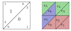
Figure 4: A coarse mesh of two trees and a uniform level 1 forest mesh. If the forest mesh is partitioned to three processes, each tree of the coarse mesh is requested by two processes. The numbers in the tree corners denote the position and orientation of the tree vertices and the global tree ids are the numbers in the center of each tree. As an example SFC we take the triangular Morton curve from [11], but the situation of multiple trees per process can occur for any SFC.

3.1 Valid partitions

We allow any SFC induced partition for the forest. This gives us some information on the type of coarse mesh partitions that we can expect as follows.

Definition 3.

In general a partition of a coarse mesh of $K$ trees $\left\{\,0,\dots,K-1\,\right\}$ to $P$ processes $\left\{\,0,\dots,P-1\,\right\}$ is a map $f$ that assigns each process a certain subset of the trees,

$$f\colon\left\{\,0,\dots,P-1\,\right\}\longrightarrow\mathcal{P}\left\{\,0,\dots,K-1\,\right\},$$ (6)

and whose image covers the whole mesh:

$$\bigcup_{p=0}^{P-1}f(p)=\left\{\,0,\dots,K-1\,\right\}.$$ (7)

Here, $\mathcal{P}$ denotes the set of all subsets (power set). We call $f(p)$ the local trees of process $p$ and explicitly allow that $f(p)\cap f(q)$ may be nonempty. If so, the trees in this intersection are shared between processes $p$ and $q$.

For a partition $f$ we denote with ${k_{p}}$ the local tree on $p$ with lowest global index and with ${K_{p}}$ the one with the highest global index.

We need not consider all possible partitions of a coarse mesh. Since we assume that a forest mesh partition comes from a space-filling curve, we can restrict ourselves to a subset of partitions.

Definition 4.

Consider a partition $f$ of a coarse mesh with $K$ trees. We say that $f$ is a valid partition if there exists a forest mesh with $N$ leaves and a (possibly weighted) SFC partition of it that induces $f$. Thus, for each process $p$ and each tree $k$ we have $k\in f(p)$ if and only if there exists a leaf $e$ of the tree $k$ in the forest mesh that is partitioned to process $p$. Processes without any trees are possible; in this case $f(p)=\emptyset$.

We deduce three properties that characterize valid partitions and lead to a definition that is independent of a forest mesh.

Proposition 5.

A partition $f$ of a coarse mesh is valid if and only if it fulfills the following properties.

1. The tree indices of a process’ local trees are consecutive, thus

   $$f(p)=\left\{\,{k_{p}},{k_{p}+1},\dots,{K_{p}}\,\right\},\,\text{ or }\,f(p)=\emptyset.$$ (8)

2. A tree index of a process $p$ may be smaller than a tree index on a process $q$ only if $p\leq q$:

   $$p\leq q\Rightarrow K_{p}\leq k_{q}\quad(\text{if}\,\,f(p)\neq\emptyset\neq f(q)).$$ (9)

3. The only trees that can be shared by process $p$ with other processes are $k_{p}$ and $K_{p}$:

   $$f(p)\cap f(q)\subseteq\left\{\,{k_{p}},{K_{p}}\,\right\},\,\text{for}\,\,p\neq q.$$ (10)

Proof.

We show the only-if direction first. So let an arbitrary forest mesh with SFC partition be given, such that $f$ is induced by it. In the SFC order the leaves are sorted according to their SFC indices. If ${(i,I)}$ denotes the leaf corresponding to the $I$-th leaf in the $i$-th tree and tree $i$ has $N_{i}$ leaves, then the complete forest mesh consists of the leaves

$$\left\{\,{(0,0)},{(0,1)},{(0,N_{0}-1)},{(1,0)},\dots,{(K-1,N_{K-1}-1)}\,\right\}.$$ (11)

The partition of the forest mesh is such that each process $p$ gets a consecutive range

$$\left\{\,{(k_{p},i_{p})},\dots,{(K_{p},i^{\prime}_{p})}\,\right\}$$ (12)

of leaves. Where $(k_{p+1},i_{p+1})$ is the successor of $(K_{p},i^{\prime}_{p})$. and the $k_{p}$ and $K_{p}$ form increasing sequences with additionally $K_{p}\leq k_{p+1}$. The coarse mesh partition is then given by

$$f(p)=\left\{\,k_{p},k_{p}+1,\dots,K_{p}\,\right\},\,\,\text{for all }p,$$ (13)

which shows properties $(i)$ and $(ii)$. To show $(iii)$ we assume that $f(p)$ has at least three elements, thus $f(p)=\left\{\,{k_{p}},{k_{p}+1},\dots,{K_{p}}\,\right\}$. However, this means that in the forest mesh partition each leaf that is a child from the trees in $\left\{\,k_{p}+1,\dots,K_{p}-1\,\right\}$ is partitioned to $p$. Since the forest mesh partitions are disjoint, no other process can hold leaf elements from these trees and thus they cannot be shared.

To show the if-direction, suppose the partition $f$ fulfills (i), (ii) and (iii). We construct a forest mesh with a weighted SFC partition as follows. Each tree that is local to a single process is not refined and thus a single leaf element in the forest mesh. If a tree is shared by $m$ processes then we refine it uniformly until we have more then $m$ elements. It is now straightforward to choose the weights of the elements such that the corresponding SFC partition induces $f$. ∎

We directly conclude:

Corollary 6.

In a valid partition each pair of processes can share at most one tree, thus

$$|f(p)\cap f(q)|\leq 1$$ (14)

for each $p\neq q$.

Proof.

Suppose not then with (10) we know that there exist two processes $p$ and $q$ with $p<q$ such that $f(p)\cap f(q)\,=\,\left\{\,{k_{p}},{K_{p}}\,\right\}=\left\{\,{k_{q}},{K_{q}}\,\right\}$ and $k_{p}\neq K_{p}$. Thus, $K_{p}>k_{p}=k_{q}$ which contradicts property (9). ∎

Corollary 7.

If in a valid partition $f$ of a coarse mesh the tree $k$ is shared between processes $p$ and $q$, then for each $p<r<q$

$$f(r)=\left\{\,k\,\right\}\quad\mathrm{or}\quad f(r)=\emptyset.$$ (15)

Proof.

We can directly deduce this from (8), (9) and Corollary 6. ∎

In order to properly deal with empty processes in our calculations, we define start and end tree indices for these as well.

Definition 8.

Let $p$ be an empty process in a valid partition $f$, thus $f(p)=\emptyset$. Let furthermore $q<p$ be maximal such that $f(q)\neq\emptyset$. Then we define the start and end indices of $p$ as

$$k_{p} :=K_{q}+1,$$ (16)

$$K_{p} :=K_{q}=k_{p}-1.$$ (17)

If no such $q$ exists, then no rank lower than $p$ has local trees and we set $k_{p}=0$, $K_{p}=-1$. With these definitions, equations (8) and (9) are valid if any of the processes are empty.

From now on all partitions in this manuscript are considered as valid even if not stated explicitly.

3.2 Encoding a valid partition

A typical way to define a partition in a tree based code is to store an array O of tree offsets for each process, that is, for process $p$ the global index of the first local tree is stored. The range of local trees for process $p$ can then be computed as $\left\{\,{\texttt{O}[p]},\dots,{\texttt{O}[p+1]-1}\,\right\}$. However, for valid partitions in the coarse mesh setting, this information would not be sufficient because we would not know which trees are shared. We thus slightly modify the offset array by adding a negative sign when the first tree of a process is shared.

Definition 9.

Let $f$ be a valid partition of a coarse mesh with $k_{p}$ being the index of $p$’s first local tree. Then we store this partition in an array O of length $P+1$, where for $0\leq p<P$

$$\texttt{O}[p]=\left\{\begin{array}[]{ll}k_{p},&\begin{array}[]{l}\textrm{if ${k_{p}}$ is not shared with the next smaller}\\ \textrm{nonempty process or }f(p)=\emptyset,\end{array}\\[8.61108pt] -k_{p}-1,&\,\,\,\textrm{if it is.}\end{array}\right.$$ (18)

Furthermore, in $\texttt{O}[P]$ we store the total number of trees.

Because of the definition of $k_{p}$ we know that $\texttt{O}[0]=0$ for all valid partitions.

Lemma 10.

Let $f$ be a valid partition and O as in Definition 9. Then

$$k_{p}=\begin{cases}\texttt{O}[p],&\textrm{if }\texttt{O}[p]\geq 0,\\[4.30554pt] |\texttt{O}[p]+1|,&\textrm{if }\texttt{O}[p]<0,\end{cases}$$ (19)

and

$$K_{p}=|\texttt{O}[p+1]|-1.$$ (20)

Proof.

The first statement follows since equations (18) and (19) are inverses of each other.

For equation (20) we distinguish two cases: First, let $f(p)$ be nonempty. If the last tree of $p$ is not shared with $p+1$, then it is ${k_{p+1}}-1$ and $\texttt{O}[p+1]=k_{p+1}$, thus we have

$$K_{p}=k_{p+1}-1=|\texttt{O}[p+1]|-1.$$ (21)

If the last tree of $p$ is shared with $p+1$, then it is $k_{p+1}$, the first local tree of $p+1$ and thus $\texttt{O}[p+1]=-k_{p+1}-1$ and

$$K_{p}=k_{p+1}=|-k_{p+1}|=|\texttt{O}[p+1]|-1.$$ (22)

Let now $f(p)=\emptyset$. If $k_{p+1}$ is not shared, then $k_{p+1}=k_{p}=K_{p}+1$ by Definition 8 and $\texttt{O}[p+1]=k_{p+1}$ by (18). Thus,

$$K_{p}=k_{p}-1=k_{p+1}-1=|\texttt{O}[p+1]|-1.$$ (23)

If $k_{p+1}$ is shared, then again by Definition 8 $k_{p+1}=k_{p}-1=K_{p}$ and $\texttt{O}[p+1]=-k_{p+1}-1$, such that we obtain

$$K_{p}=k_{p+1}=k_{p+1}+1-1=|\texttt{O}[p+1]|-1.$$ (24)

∎

Corollary 11.

In the setting of Lemma 10 the number $n_{p}$ of local trees of process $p$ fulfills

$$n_{p}=|\texttt{O}[p+1]|-k_{p}=\begin{cases}|\texttt{O}[p+1]|-\texttt{O}[p],&\textrm{if }\texttt{O}[p]\geq 0\\ |\texttt{O}[p+1]|-|\texttt{O}[p]+1|,&\textrm{else.}\end{cases}$$ (25)

Proof.

This follows from the formula $n_{p}=K_{p}-k_{p}+1$. ∎

Lemma 10 and Corollary 11 show that for valid partitions the array O carries the same information as the partition $f$.

3.3 The ghost trees

A valid partition gives the information about the local trees of a process. These trees are all trees from whom a forest has local elements. In many applications it is necessary to create a layer of ghost (or halo) elements of the forest to properly exchange data with the neighboring processes. Since these ghost elements may be descendants of non local trees, we also want to store those trees as ghost trees. To be independent of a forest mesh we store each possible ghost tree and do not consider whether there are actually forest mesh ghost elements in this tree. This, however, does only affect the first and the last local tree, where we possibly store more ghosts than needed by a forest. Since we restrict the neighbor information to face-neighbors, we also restrict ourselves to face-neighbor ghosts in this paper.

Definition 12.

Let $f$ be a valid partition of a coarse mesh. A ghost tree of a process $p$ is any tree $k$ such that

• $k\notin f(p)$, and

• There exists a face-neighbor $k^{\prime}$ of $k$, such that $k^{\prime}\in f(p)$.

If a coarse mesh is partitioned according to $f$ then each process $p$ will store its local trees and its ghost trees.

3.4 Computing the communication pattern

Suppose we are in a setting where a coarse mesh is partitioned among the processes $p\in\left\{\,0,\dots,P-1\,\right\}$ according to a partition $f$. The input of the partition algorithm is this coarse mesh and a second partition $f^{\prime}$, and the output is a coarse mesh that is partitioned according to the second partition.

We suppose that besides its local trees and ghosts each process knows the complete partition tables $f$ and $f^{\prime}$, for example in the form of offset arrays. The task is now for each process to identify the processes that it needs to send local trees and ghosts to and carry out this communication. A process also needs to identify the processes it receives trees and ghosts from and do the receiving. We discuss here how each process can compute this information from the offset arrays without further communication.

3.4.1 Ownership during partition

The fact that trees can be shared between multiple processes poses a challenge when repartitioning a coarse mesh. Suppose we have a process $p$ and a tree $k$ with $k\in f^{\prime}(p)$, and $k$ is a local tree for more than one process in the partition $f$. We do not want to send the tree multiple times, so how do we decide which process sends $k$ to $p$?

A simple solution would be that the process with the smallest index that $k$ is a local tree to sends $k$. This process is unique and it can be determined without communication. However, suppose that the two processes $p$ and $p-1$ share the tree $k$ in the old partition and $p$ will also have this tree in the new partition. Then $p-1$ would send the tree to $p$ even though we could handle this situation without any communication.

We solve this by only sending a local tree to a process $p$ if this tree was not already local on $p$:

Paradigm 13.

In a repartitioning setting with $k\in f^{\prime}(p)$, the process that sends $k$ to $p$ is

• $p$, if $k$ already is a local tree of $p$, or else

• $q$, with $q$ minimal such that $k\in f(q)$.

We acknowledge that sending from $p$ to $p$ in the first case is just a local data movement involving no communication.

Definition 14.

In a repartitioning setting, given a process $p$ we define the sets $S_{p}$ and $R_{p}$ of processes that $p$ sends local trees to, resp. receives from, thus

$$S_{p} :=\left\{\,0\leq p<P\,|\,p\textrm{ sends local trees to p'}\,\right\},$$ (26a)

$$R_{p} :=\left\{\,0\leq p<P\,|\,p\textrm{ receives local trees from p'}\,\right\}.$$ (26b)

These sets can both include the process $p$ itself. Furthermore, we establish notations for the smallest and biggest ranks in these sets:

$$s_{\mathrm{first}}:=\min S_{p}, \quad s_{\mathrm{last}}:=\max S_{p},$$ (27a)

$$r_{\mathrm{first}}:=\min R_{p}, \quad r_{\mathrm{last}}:=\max R_{p}.$$ (27b)

$S_{p}$ and $R_{p}$ are uniquely determined by Paradigm 13.

3.4.2 An example

We discuss a small example, see Figure 5. Here, we repartition a partitioned coarse mesh of five trees among three processes. We color the local trees of process $0$ in blue, the local trees of process $1$ in green and the local trees of process $2$ in red. The initial partition $f$ is given by

$$\texttt{O}=\left\{\,0,-2,3,5\,\right\},$$ (28)

and the new partition $f^{\prime}$ by

$$\texttt{O'}=\left\{\,0,-3,-4,5\,\right\}.$$ (29)

Thus, initially tree $1$ is shared by processes $0$ and $1$ and in the new partition tree $2$ is shared by processes $0$ and $1$ and tree $3$ by processes $2$ and $3$. We give the local trees that each process will send to each other process in a table, where the set in row $i$ column $j$ is the set of local trees that process $i$ send to process $j$.

$$\begin{array}[]{c|ccc}&0&1&2\\ \hline\cr 0&\left\{\,0,1\,\right\}&\emptyset&\emptyset\\ 1&\left\{\,2\,\right\}&\left\{\,2\,\right\}&\emptyset\\ 2&\emptyset&\left\{\,3\,\right\}&\left\{\,3,4\,\right\}\end{array}$$ (30)

This leads to the sets $S_{p}$ and $R_{p}$:

$$S_{0} =\left\{\,0\,\right\}, R_{0} =\left\{\,0,1\,\right\},$$ (31a)

$$S_{1} =\left\{\,0,1\,\right\}, R_{1} =\left\{\,1,2\,\right\},$$ (31b)

$$S_{2} =\left\{\,1,2\,\right\}, R_{2} =\left\{\,2\,\right\}.$$ (31c)

For example process $1$ keeps the tree $2$ that is also needed by process $0$. Thus, process $1$ sends tree $2$ to process $0$. Process $0$ also needs tree $1$, which is local on process $1$ in the old partition. But, since it is also local to process $0$, process $1$ does not send it.

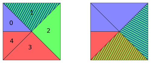
Figure 5: A small example for coarse mesh partitioning. The coarse mesh consists of 5 trees and is partitioned among three processes. Left: The initial partition O. Right: The new partition O’. The colors of the trees encode the processes that have the respective tree as local tree. Process $0$ in blue, process $1$ in green, and process $2$ in red. Thus, initially tree 1 is shared among processes $0$ and $1$ and in the new partition tree 2 is shared among processes $0$ and $1$, and tree 3 among processes $1$ and $2$. In equations (28)-(31) we depict the sets O and O’, the trees that each process sends, and the sets $S_{p}$ and $R_{p}$.

3.4.3 Determining $S_{p}$ and $R_{p}$

In this section we show that each process can compute the sets $S_{p}$ and $R_{p}$ from the offset array without further communication. It will become clear in Section 3.5 that ghost trees need not yet be discussed at this point.

Proposition 15.

A process $p$ can calculate the sets $S_{p}$ and $R_{p}$ without further communication from the offset arrays of the new and old partition. Once the first and last element of each set are known, $p$ can determine in constant time whether any given rank is in any of those sets.

We split the proof in two parts. First we discuss how a process can compute $s_{\mathrm{first}},\,s_{\mathrm{last}},\,r_{\mathrm{first}},$ and $r_{\mathrm{last}}$, and then how it can decide for two processes $\tilde{p}$ and $q$ whether $q\in S_{\tilde{p}}$.

We derive $S_{p}$ from $s_{\mathrm{first}}$ and $s_{\mathrm{last}}$. To determine $s_{\mathrm{first}}$ we consider two cases. First, if the first local tree of $p$ is not shared with a smaller rank, then $s_{\mathrm{first}}$ is the smallest process that has this tree in the new partition and did not have it in the old one. We can find this process with a binary search in the offset array.

Second, if the first tree of $p$ is shared with a smaller rank, then $p$ only sends it in the case that $p$ keeps this tree in the new partition. Then $s_{\mathrm{first}}=p$. Otherwise, we consider the second tree of $p$ and proceed with a binary search as in the first case.

To compute $s_{\mathrm{last}}$ we notice that among all ranks having $p$’s old last tree in the new partition that did not already have it before, $s_{\mathrm{last}}$ is the biggest (except when $p$ itself is this biggest rank, in which case it certainly had the last tree before). We can determine this rank with a binary search as well. If no such process exists, we proceed with the second last tree of $p$.

Remark 16.

The special case when $S_{p}=\emptyset$ occurs under three circumstances:

1. $p$ does not have any local trees.

2. $p$ only has one local tree, it is shared with a smaller rank, and $p$ does not have this tree as a local tree in the new partition.

3. $p$ only has two trees, for the first one case 2 holds and the second ($=$last) one is shared with a set $Q$ of bigger ranks. There is no process $q\notin Q$ that has this tree as a local tree in the new partition.

These conditions can be queried before computing $s_{\mathrm{first}}$ and $s_{\mathrm{last}}$.

Similarly, to compute $R_{p}$, we first look at the smallest and biggest elements of this set. These are the first and last process that $p$ receives trees from. $r_{\mathrm{first}}$ is the smallest rank that had $p$’s new first tree as a local tree in the old partition, or it is $p$ itself if this tree was also a local tree on $p$. And $r_{\mathrm{last}}$ is the smallest rank bigger then $r_{\mathrm{first}}$ that had $p$’s new last local tree as a local tree in the old partition, or $p$ itself. We can find both of these with a binary search in the offset array of the old partition.

Remark 17.

$R_{p}$ is empty if and only if $p$ does not have any local trees in the new partition.

Lemma 18.

Given any two processes $\tilde{p}$ and $q$ the process $p$ can determine in constant time whether $q\in S_{\tilde{p}}$. In particular, this includes the cases $\tilde{p}=p$ and $q=p$.

Proof.

Let $\hat{k}_{\tilde{p}}$ be the first non-shared local tree of $\tilde{p}$ in the old partition. Let $\hat{K}_{\tilde{p}}$ be the last local tree of $\tilde{p}$ in the old partition if it is not the first local tree of $q$ in the old partition. Let it be the second last local tree otherwise. Furthermore, let $\hat{k}_{q}$ and $\hat{K}_{q}$ be the first, resp. last, local trees of $q$ in the new partition. We add $1$ to $\hat{k}_{q}$ if $q$ sends its first local tree to itself and this tree is also the new first local tree of $q$. We claim that $q\in S_{\tilde{p}}$ if and only if all of the four inequalities

$$\hat{k}_{\tilde{p}}\leq\hat{K}_{\tilde{p}},\quad\hat{k}_{\tilde{p}}\leq\hat{K}_{q},\quad\hat{k}_{q}\leq\hat{K}_{\tilde{p}},\quad\textrm{and}\quad\hat{k}_{q}\leq\hat{K}_{q}\phantom{,}$$ (32)

hold. The only-if direction follows, since if $\hat{k}_{\tilde{p}}>\hat{K}_{\tilde{p}}$, then $\tilde{p}$ does not have trees to send to $q$. If $\hat{k}_{\tilde{p}}>\hat{K}_{q}$, then the last new tree on $q$ is smaller than the first old tree on $\tilde{p}$. If $\hat{k}_{q}>\hat{K}_{\tilde{p}}$ then the last tree that $\tilde{p}$ could send is smaller than the first new local tree of $p$. And if $\hat{k}_{q}>\hat{K}_{q}$ then $q$ does not receive any trees from other processes. Thus $\tilde{p}$ cannot send trees to $q$ if any of the four conditions is not fulfilled. The if-direction follows, since if all four conditions are fulfilled there exist at least one tree $k$ with

$$\hat{k}_{\tilde{p}}\leq k\leq\hat{K}_{\tilde{p}}\quad\mathrm{and}\quad\hat{k}_{q}\leq k\leq K_{q}.$$ (33)

Any tree with this properties is sent from $\tilde{p}$ to $q$. Process $p$ can compute the four values $\hat{k}_{\tilde{p}},\hat{K}_{\tilde{p}},\hat{k}_{q}$ and $\hat{K}_{q}$ from the partition offsets in constant time. ∎

Remark 19.

Let $p$ be a process that is not empty in the new partition. For symmetry reasons, $R_{p}$ contains exactly those processes $\tilde{p}$ with $r_{\mathrm{first}}\leq\tilde{p}\leq r_{\mathrm{last}}$ and $p\in S_{\tilde{p}}$.

Thus, in order to compute $S_{p}$, we can compute $s_{\mathrm{first}}$ and $s_{\mathrm{last}}$ and then check for each rank $q$ in between whether the conditions of Lemma 18 are fulfilled with $\tilde{p}=p$. For each process this check only takes constant run time.

Now, to compute $R_{p}$ we can compute $r_{\mathrm{first}}$ and $r_{\mathrm{last}}$, and then check for each rank $q$ in between whether $p\in S_{q}$.

These considerations provide the proof for Proposition 15.

3.5 Face information for ghost trees

We identify five different types of possible face connections in a coarse mesh:
1. Local tree to local tree. 2. Local tree to ghost tree. 3. Ghost tree to local tree. 4. Ghost tree to ghost tree. 5. Ghost tree to non-local and non-ghost tree.
There are several possible approaches to which of these face connections of a local coarse mesh we could actually store. As long as each face connection between any two neighbor trees is stored at least once globally, the information of the coarse mesh over all processes is complete, and a single process could reproduce all five types of face connection at any time, possibly using communication. Depending on which of these types we store, the pattern for sending and receiving ghost trees during repartitioning changes. Specifically, the trees that will become a ghost on the receiving process may be either a local tree or a ghost on the sending process.

When we use the maximum possible information of all five connections, we have the most data available and can minimize the communication required. In particular, from the non-local neighbors of a ghost and the partition table a process can compute which other processes this ghost is also a ghost of and of which it is a local tree. With this information we can ensure that a ghost is only sent once and only from a process that also sends local trees to the receiving process.

The outline of the sending/receiving phase of the partition algorithm then looks like this:

1. For each $q\in S_{p}$: Send local trees that will be owned by $q$ (following Paradigm 13).

2. Consider sending a neighbor of these trees to $q$ if it will be a ghost on $q$. Send one of these neighbors if both

   • $p$ is the smallest rank among those that consider sending this neighbor as a ghost, and

   • $p\neq q$ and $q$ does not consider sending this neighbor as a ghost to itself.

3. For each $q\in R_{p}$: Receive the new local trees and ghosts from $q$.

In step 2 a process needs to know, given a ghost that is considered for sending to $q$, which other processes consider sending this ghost to $q$. This can be calculated without further communication from the face-neighbor information of the ghost. Since we know for each ghost the global index of each of its neighbors, we can check whether any of these neighbors is currently local on a different process $\tilde{p}$ and will be sent to $q$ by $\tilde{p}$. If so, we know that $\tilde{p}$ considers sending this ghost to $q$.

Using this method, each local tree and ghost is sent only once to each receiver, and only those processes send that send local trees anyway, thus we have a minimum number of communications and data movement. Storing less information would either increase the number of communicating processes or the amount of data that is communicated.

Suppose we would not store the face connection type 5, thus for ghost trees we do not have the information with which non-local trees it is connected. With this face information we can use a communication pattern such that each ghost is only received once by a process $q$, by sending the new ghost trees from a process that currently has it as a local tree (taking Paradigm 13 into account). However, this designated process might not be an element of $R_{q}$, in which case additional processes would communicate.

If we only store the local tree face information, types 1 and 2, then we have minimal control over the ghost face connections. Nevertheless, we can define the partition algorithm by specifying that if a process $p$ sends local trees to a process $q$, it will send all neighbors of these local trees as potential ghosts to $q$. The process $q$ is then responsible for deleting those trees that it received more than once. With this method the number of communicating processes would be the same but the amount of data communicated would increase.

	1, 2			1, 2, 3, 4			1, 2, 3, 4, 5
p	0	1	2	0	1	2	0	1	2
0	0(1,2)	0(2)	—	0	0	(0)	0(1,2)	0	—
1	—	1(2)	2(0,1)	(1,2)	1(2)	2(1)	—	1(2)	2 (0,1)

Figure 6: Repartitioning example of a coarse mesh showing the communication patterns controlled by the amount of face information available. Top: A coarse mesh of three trees is repartitioned. The numbers outside of the trees are their global indices. The numbers inside of each tree denote the processes that have this tree as a local tree. At first process 0 has tree 0, process 1 trees 1 and 2, and process 2 no trees as local trees. After repartitioning process 0 has tree 0, process 1 trees 0 and 1, and process 2 tree 2 as local trees. Bottom: The table shows for each usage of face connection types which processes send which data. The row of process $i$ shows in column $j$ which local trees $i$ sends to $j$, and—in parentheses—which ghosts it sends to $j$. Using face connection types 1–4 we use more communication partners (process 0 sends to process 2 and process 1 to process 0) than with all five types. Using types 1 and 2 only, duplicate data is sent (process 0 and process 1 both send the ghost tree 2 to process 1).

We give an example comparing the three face information strategies in Figure 6. To minimize the communication and overcome the need for postprocessing steps, it is thus recommended to store all five types of face connections.

4 Implementation

Let us begin by outlining the main data structures for trees, ghosts, and the coarse mesh, and continue with a section on how to update the local tree and ghost indices. After this we present the partition algorithm to repartition a given coarse mesh according to a pre-calculated partition array. We emphasize that the coarse mesh data stores pure connectivity. In particular, it does not include the forest information, that is leaf elements and per-element payloads, which are managed by separate, existing algorithms.

4.1 The coarse mesh data structure

Our data structure cmesh that describes a (partitioned) coarse mesh has the entries:

• O — An array storing the current partition table, see Definition 9.

• $n_{p}$ — The number of local trees on this process.

• $n_{\mathrm{ghosts}}$ — The number of ghost trees on this process.

• trees — A structure storing the local trees in order of their global index.

• ghosts — A structure storing the ghost trees in no particular order.

We use $32$-bit signed integers for the local tree counts in trees and ghosts and $64$-bit integers for global counts in O. This limits the number of trees per process to $2^{31}-1\cong 2\times 10^{9}$. However, even with an overly optimistic memory usage of only $10$ bytes per tree, storing that many trees would require about $18.6$GB of memory per process. Since on most distributed machines the memory per process is indeed much smaller, restricting to $32$-bit integers does not effectively limit the local number of trees. In presently unimaginable cases, we can still switch to $64$-bit integers.

We call the index of a local tree inside the trees array the local index of this tree. Analogously, we call the index of a ghost in ghosts the local index of that ghost. On process $p$, we compute the global index $k$ of a tree in trees from its local index $\ell$ and the global index $k_{p}$ of the first local tree and vice versa, since

$$k=k_{p}+\ell.$$ (34)

This allows us to address local trees with their local indices using $32$-bit integers.

Each tree in the array trees stores the following data:

• eclass — The tree’s type as a small number (triangle, quadrilateral, etc.).

• tree_to_tree — An array storing the local tree and ghost neighbors along this tree’s faces. See Section 2.2.

• tree_to_face — An array encoding for each face the neighbor face number and the orientation of the face connection. See Section 2.3.

• tree_data — A pointer to additional data that we store for the tree, for example geometry information or boundary conditions defined by an application.

The $i$-th entry of tree_to_tree array encodes the tree number of the face-neighbor at face $i$ using an integer $k$ with $0\leq k<n_{p}+n_{\mathrm{ghosts}}$. If $k<n_{p}$, the neighbor is the local tree with local index $k$. Otherwise the neighbor is the ghost with local index $k-n_{p}$.

We do not allow a face to be connected to itself. Instead, we use such a connection in the face-neighbor array to indicate a domain boundary. However, a tree can be connected to itself via two different faces. This allows for one-tree periodicity, as say in a 2D torus consisting of a single square tree.

Each ghost in the array ghosts stores the following data:

• Id — The ghost’s global tree index.

• eclass — The type of the ghost tree.

• tree_to_tree — An array giving for each face the global number of its face-neighbor.

• tree_to_face — As above.

Since a ghost stores the global number of all of its face-neighbor trees, we can locally compute all other processes that have this tree as a ghost by combining the information from O and tree_to_tree.

4.2 Updating local indices

After partitioning, the local indices of the trees and ghosts change. The new local indices of the local trees are determined by subtracting the global index of the first local tree from the global index of each local tree. The local indices of the ghosts are given by their position in the data array.

Since the local indices change after repartitioning, we update the face-neighbor entries of the local trees to store those new values. Because a neighbor of a tree can either be a local tree or a ghost on the previously owning process $\tilde{p}$ and become either a tree or a ghost on the new owning process $p$, there are four cases that we shall consider.

We handle these four cases in two phases, the first phase is carried out on process $\tilde{p}$ before the tree is sent to $p$. In this phase we change all neighbor entries of the trees that become local. The second phase is done on $p$ after the tree was received from $\tilde{p}$. Here we change all neighbor entries belonging to trees that become ghosts.

In the first phase, $\tilde{p}$ has information about the first local tree on $\tilde{p}$ in the old partition, its global number being $k_{\tilde{p}}$. Via O’ it also knows $k_{p}^{\mathrm{new}}$, the global index of $p$’s first tree in the new partition. Given a local tree on $\tilde{p}$ with local index $\tilde{k}$ in the old partition we compute its new local index $k$ on $p$ as

$$k=k_{\tilde{p}}+\tilde{k}-k_{p}^{\mathrm{new}},$$ (35)

which is its global index minus the global index of the new first local tree. Given a ghost $g$ on $\tilde{p}$ that will be a local tree on $p$, we compute its local tree number as

$$k=g.\mathrm{Id}-k_{p}^{\mathrm{new}}.$$ (36)

In the second phase $p$, has received all its new trees and ghosts and thus can give the new ghosts local indices to be stored in the neighbors fields of the trees. We do this by parsing, for each process $\tilde{p}\in R_{p}$ (in ascending order), its ghosts and increment a counter. For each ghost we parse its neighbors for local trees, and for any of these we set the appropriate value in its neighbors field.

4.3 Partition_cmesh — Algorithm 4.1

The input is a partitioned coarse mesh $C$ and a new partition layout O’, and the output is a new coarse mesh $C^{\prime}$ that carries the same information as $C$ and is partitioned according to O’.

This algorithm follows the method described in Section 3.5 and is separated in two main phases, the sending phase and the receiving phase. In the former we iterate over each process $q\in S_{p}$ and decide which local trees and ghosts we send to $q$. Before sending, we carry out phase one of the update of the local tree numbers. Subsequently, we receive all trees and ghosts from the processes in $R_{p}$ and carry out phase two of the local index updating.

In the sending phase we iterate over the trees that we send to $q$. For each of these trees we check for each neighbor (local tree and ghost) whether we send it to $q$ as a ghost tree. This is the item 2 in the list of Section 3.5. The function Parse_neighbors decides for a given local tree or ghost neighbor whether it is sent to $q$ as a ghost.

1 $p\leftarrow$ this process

From C.O and O’ determine $S_{p}$ and $R_{p}$.

  /* See Section 3.4.3 */

2

 /* Sending phase */

3

4for each $q\in S_{p}$ do

       $G\leftarrow\emptyset$

        /* trees $p$ sends as ghosts to $q$ */

5      

6      $s\leftarrow$ first local tree to send to $q$.

7      $e\leftarrow$ last local tree to send to $q$.

      $T\leftarrow\left\{\,C.\texttt{trees}[s],\dots,C.\texttt{trees}[e]\,\right\}$

        /* local trees $p$ sends to $q$ */

8      

9      for $k\in T$ do

10             Parse_neighbors ($C$, $k$, $p$, $q$, $G$, O’)

      update_tree_ids_phase1 $(T\cup G)$

        /* See equations (35) and (36) */

11      

12      Send $T\cup G$ to process $q$

13

 /* Receiving phase */

14 for each $q\in R_{p}$ do

15       Receive $T[q]\cup G[p]$ from process $p$

16

$C^{\prime}.\mathrm{trees}\leftarrow\displaystyle\bigcup_{R_{p}}T[q]$

  /* The updated tree array */

17

$C^{\prime}.\mathrm{ghosts}\leftarrow\displaystyle\bigcup_{R_{p}}G[q]$

  /* The updated ghost array */

18

19update_tree_ids_phase2 $(C.\mathrm{ghosts})$

20$C^{\prime}.\texttt{O}\leftarrow\texttt{O'}$

21return C’  

 /* decide which neighbors of $k$ to send as a ghost to $q$ */

1 Function Parse_neighbors(cmesh $C$, tree $k$, processes $p$, $q$, Ghosts $\ast G$, partition O’)

2for $u\in k.\texttt{tree\_to\_tree}\backslash\left\{\,C.\texttt{trees}[s],\dots,C.\texttt{trees}[e]\,\right\}$  do

3       if $0\leq u<k_{p}$ $\textbf{ and }\texttt{Send\_ghost}(C,\texttt{ghost}(u),q,\texttt{O'})$ then

4             if $u+k_{p}\notin f^{\prime}(q)$ then

                   $G\leftarrow G\cup\left\{\,\texttt{ghost}(u)\,\right\}$

                    /* local tree $u$ gets ghost of $q$ */

5                  

6            

7      else /* $k_{p}\leq u$ */

8             $g\leftarrow C.\mathrm{ghosts}[u-n_{p}]$ if $g.Id\notin f(q)$ and Send_ghost$(C,g,q,\texttt{O'})$ then

                   $G\leftarrow G\cup\left\{\,g\,\right\}$

                    /* $g$ is a ghost of $q$ */

9                  

10            

11      

 

 /* Subroutine to decide whether to send a ghost or not */

1 Function Send_ghost(cmesh $C$, ghost $g$, process $q$, partition O’) $S\leftarrow\emptyset$

2 for $u\in g.\texttt{tree\_to\_tree}$ do

3       for $q^{\prime}$ with $u$ is a local tree of $q^{\prime}$ do

4             if $q^{\prime}$ sends $u$ to $q$ then

5                   $S\leftarrow S\cup\left\{\,q^{\prime}\,\right\}$

6            

7      

8if $q\notin S$ and $p=\min S$ then

       return True

        /* $p$ is the smallest rank sending trees to $q$ */

9      

10else

11       return False

Algorithm 4.1 Partition_cmesh(cmesh $C$, partition O’)

5 Numerical Results

The run time results that we present here have been obtained using the Juqueen supercomputer at Forschungszentrum Jülich, Germany. It is an IBM BlueGene/Q system with 28,672 nodes consisting of IBM PowerPC A2 processors at 1.6 GHZ with 16 GB RAM per node [14]. Each compute node has 16 cores and is capable of running up to 64 MPI processes using multithreading.

5.1 How to obtain example meshes

To measure the performance and memory consumption of the algorithms presented above, we would like to test the algorithms on coarse meshes that are too big to fit into the memory of a single process, which is 1 GB on Juqueen if we use 16 MPI ranks per node. We consider three approaches to do construct such meshes:

1. Use an external parallel mesh generator.

2. Use a serial mesh generator on a large-memory machine, transfer the coarse mesh to the parallel machine’s file system, and read it using (parallel) file I/O.

3. Create a big coarse mesh by forming the disjoint union of smaller coarse meshes over the individual processes.

Due to a lack of availability of open source parallel mesh generators we restrict ourselves to the second and third method. These have the advantage that we can start with initial coarse meshes that fit into a single process’ memory, such that we can work with serial mesh generating software. In particular we use gmsh, Tetgen and Triangle for simplicial meshes [19, 35, 36].

The third method is especially well suited for weak scaling studies. The small coarse meshes can be created programmatically, communication-free on each process, which we exploit below for tests with hexahedral trees. They may be of same or different sizes between the processes. In the former approach, the number of local trees is, by definition, the same on each process.

We discuss two examples below: one examining purely the coarse mesh partitioning without regard for a forest and its elements, and another in which we drive the coarse mesh partitioning by a dynamically changing forest of elements. The latter manages shared trees and thus fully executes the algorithmic ideas put forward above.

5.2 Disjoint bricks

In our first example we conduct a strong and weak scaling study of coarse mesh partitioning and test the maximal number of cubical trees that we can support before running out of memory. To obtain reliable weak scaling results, we keep the same per-process number of trees while increasing the total number of processes. We achieve this by constructing an $n_{x}\times n_{y}\times n_{z}$ brick of cubical trees on each process, using three constant parameters $n_{x},n_{y}$ and $n_{z}$. We repartition this coarse mesh once, by the rule that each rank $p$ sends 43% of its local trees to the rank $p+1$ (except the biggest rank $P-1$, which keeps all its local trees). We choose this odd percentage to create non-trivial boundaries between the regions of trees to keep and trees to send. See Figure 7 for a depiction of the partitioned coarse mesh on six processes. The local bricks are created locally as p4est connectivities with p4est_connectivity_new_brick and are then reinterpreted in parallel as a distributed coarse mesh data structure.

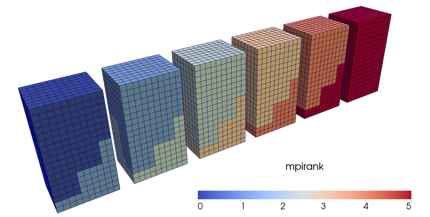
Figure 7: Depicting the structure of the coarse mesh for an example with six processes that we use to measure the maximum possible mesh sizes and scalability. Before partitioning, the coarse mesh local to each process is created as one $n_{x}\times n_{y}\times n_{z}$ block of cubical trees. We repartition the mesh such that each process sends 43% of its local trees to the next process. The picture shows the resulting partitioned coarse mesh with parameters $n_{x}=10,n_{y}=18$ and $n_{z}=8$ and color coded MPI rank.

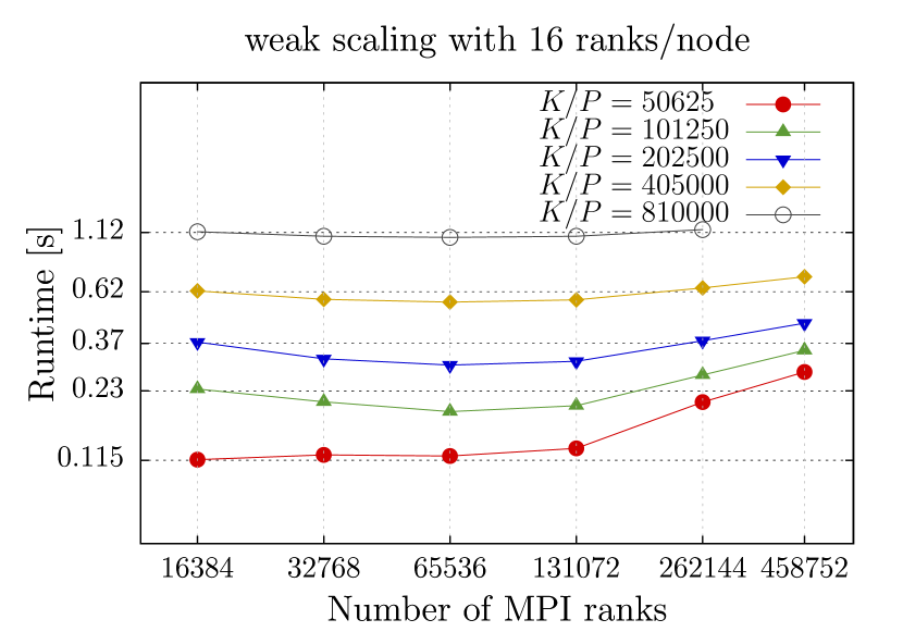
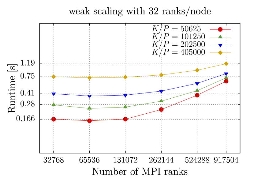
Figure 8: Weak scaling of partition with disjoint bricks. Left: 16 ranks per node. Right: 32 ranks per node. We show the run times for the baseline on the y-axis. On the left hand side the run time for the biggest 262,144-process run is 1.15 seconds, and the run time for the biggest 458,752 run is 0.719 seconds. We obtain an efficiency of 97.4%, resp. 86.2% compared to the baseline of 16,384 MPI ranks.

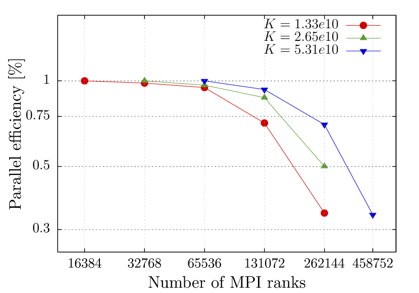
Figure 9: Strong scaling of Partition_cmesh for the disjoint bricks example on Juqueen with 16 ranks per compute node, for three runs with 1.33e10, 2.65e10, and 5.31e10 coarse mesh elements. We show the parallel efficiency on the left and the speedup on the right. The absolute run times for 262,144 processes are 0.206, 0.270 and 0.380 seconds.

Run time tests for Partition_cmesh
${X^{X}}^{X}$131072 MPI ranks (16 ranks per node)
${X^{X}}^{X}$mesh size	per rank	trees (ghosts) sent	Time [s]	Factor
${X^{X}}^{X}$6,635e9	50,625	21,768 (3,414)	0.13	–
1,327e10	101,250	43,537 (5,504)	0.20	1.53
2,654e10	202,500	87,074 (6,607)	0.31	1.56
5,308e10	405,000	174,149 (11,381)	0.57	1.85
1,062e11	810,000	348,297 (22,335)	1.08	1.89
917504 MPI ranks (32 ranks per node)
${X^{X}}^{X}$mesh size	per rank	trees (ghosts) sent	Time [s]	Factor
${X^{X}}^{X}$4.645e10	50,625	21,768 (3,413)	0.64	–
${X^{X}}^{X}$9.290e10	101,250	43,537 (5,504)	0.72	1.13
${X^{X}}^{X}$1.858e11	202,500	87,075 (6,607)	0.84	1.12
${X^{X}}^{X}$3,716e11	405.000	174,150 (11,383)	1.19	1.42

Table 1: The run times of Partition_cmesh for 131,072 processes with 16 processes per node (top) and 917,504 processes with 32 processes per node (bottom). The biggest coarse mesh that we created during the tests has 371 Billion trees. The last column is the quotient of the current run time divided by the previous run time. Since we double the mesh size in each step, we would expect an increase in run time of a factor of 2, which hints at parallel overhead becoming negligible in the limit of many elements per process.

We perform strong and weak scaling studies on up to 917,504 MPI ranks and display our results in Figures 8 and 9 and Table 1. We show the results of one study with 16 MPI ranks per compute node, thus 1GB available memory per process, and one with 32 MPI ranks per compute node, leaving half of the memory per process. In both cases we measure run times for different mesh sizes per process. We observe that even for the biggest meshes of 405k resp. 810k coarse mesh elements per process the absolute run times of partition are below 1.2 seconds. Furthermore, we measure a weak scaling efficiency of 97.4% for the 810k mesh on 262,144 processes and 86.2% for the 405k mesh on 458,752 processes. The biggest mesh that we created is partitioned between 917,504 processes and uses 405k mesh elements per process for a total of over 371e9 coarse mesh elements.

Additionally, in Table 2 we show run times for Partition_cmesh with small coarse meshes, where the number of elements is roughly on the order of the number of processes. These tests show that for such small meshes the run times are in the order of milliseconds. Hence, for small meshes there is no disadvantage in using a partitioned coarse mesh over a replicated one, when each process holds a full copy.

# MPI ranks	mesh elements	run time [s]
1024	4096	0.00136
1024	8192	0.00149
1024	16384	0.00142
64	105	0.00122
32	105	0.00789
64	3200	0.000293
64	19200	0.000865

Table 2: Run times for Partition_cmesh for relatively small coarse meshes. The bottom part of the table was not computed on Juqueen but on a local institute cluster of 78 nodes with 8 Intel Xeon CPU E5-2650 v2 @ 2.60GHz each.

5.3 An example with a forest

In this example we partition a tetrahedral coarse mesh according to a parallel forest of fine elements. Opposed to the previous test, where we exploited the maximum possible coarse element numbers, we now test mesh sizes that can occur in realistic use cases.

When simulating shock waves or two-phase flows, there is often an interface along which a finer mesh resolution is desired in order to minimize computational errors. Motivated by this example, we create the forest mesh as an initial uniform refinement of the coarse mesh with a specified level $\ell$ and refine it in a band along an interface defined by a plane in ${\mathbb{R}}^{3}$ up to a maximum refinement level $\ell+k$. As refinement rule we use 1:8 red refinement [6] together with the tetrahedral Morton space-filling curve [11]. We move the interface through the domain with a constant velocity. Thus, in each time step the mesh is refined and coarsened, and therefore we repartition it to maintain an optimal load-balance. We measure run times for both coarse mesh and forest mesh partitioning for three time steps.

Our coarse mesh consists of tetrahedral trees modelling a brick with spherical holes in it. To be more precise, the brick is built out of $n_{x}\times n_{y}\times n_{z}$ tetrahedralized unit cubes and each of those has one spherical hole in it; see Figures 10 and 11 for a small example mesh.

We create the mesh in serial using the generator gmsh [19]. We read the whole file on a single process, and thus use a local machine with 1 terabyte memory for preprocessing. On this machine we partition the coarse mesh to several hundred processes and write one file for each partition. This data is then transferred to the supercomputer. The actual computation consists of reading the coarse mesh from files, creating the forest on it, and partitioning the forest and the coarse mesh simultaneously. To optimize memory while loading the coarse mesh, we open at most one partition file per compute node.

The coarse mesh that we use in these tests has parameters $n_{x}=26,n_{y}=24,n_{z}=18$, thus 11,232 unit cubes. Each cube is tetrahedralized with about 34,150 tetrahedra, and the whole mesh consists of 383,559,464 trees. In the first test, we create a forest of uniform level 1 and maximal refinement level 2, and in the second a forest of uniform level 2 and maximal refinement level 3. The forest mesh in the first test consists of approximately 2.6e9 elements. In the second test we also use a broader band and obtain a forest mesh of 25e9 tetrahedra.

We show the run time results and further statistics for coarse mesh partitioning in Table 3 and results for forest partitioning in Table 4. We observe that the run time for Partition_cmesh is between $0.10$ and $0.13$ seconds, and that about 88%, respectively 98%, of all processes share local trees with other processes. The run times for forest partition are below $0.22$ seconds for the first example and below $0.65$ seconds for the second example. Thus, the overall run time for a complete mesh partition is below $0.5$ seconds for the first and below $1$ second for the second example.

We also run a third test on 458,752 MPI ranks and refine the forest to a maximum level of four. Here, the forest mesh has 167e9 tetrahedra, which we partition in under 0.6 seconds. The coarse mesh partition routine runs in about 0.2 seconds. Approximately 60% of the processes have a shared tree in the coarse mesh. We show the results from this test in Table 5.

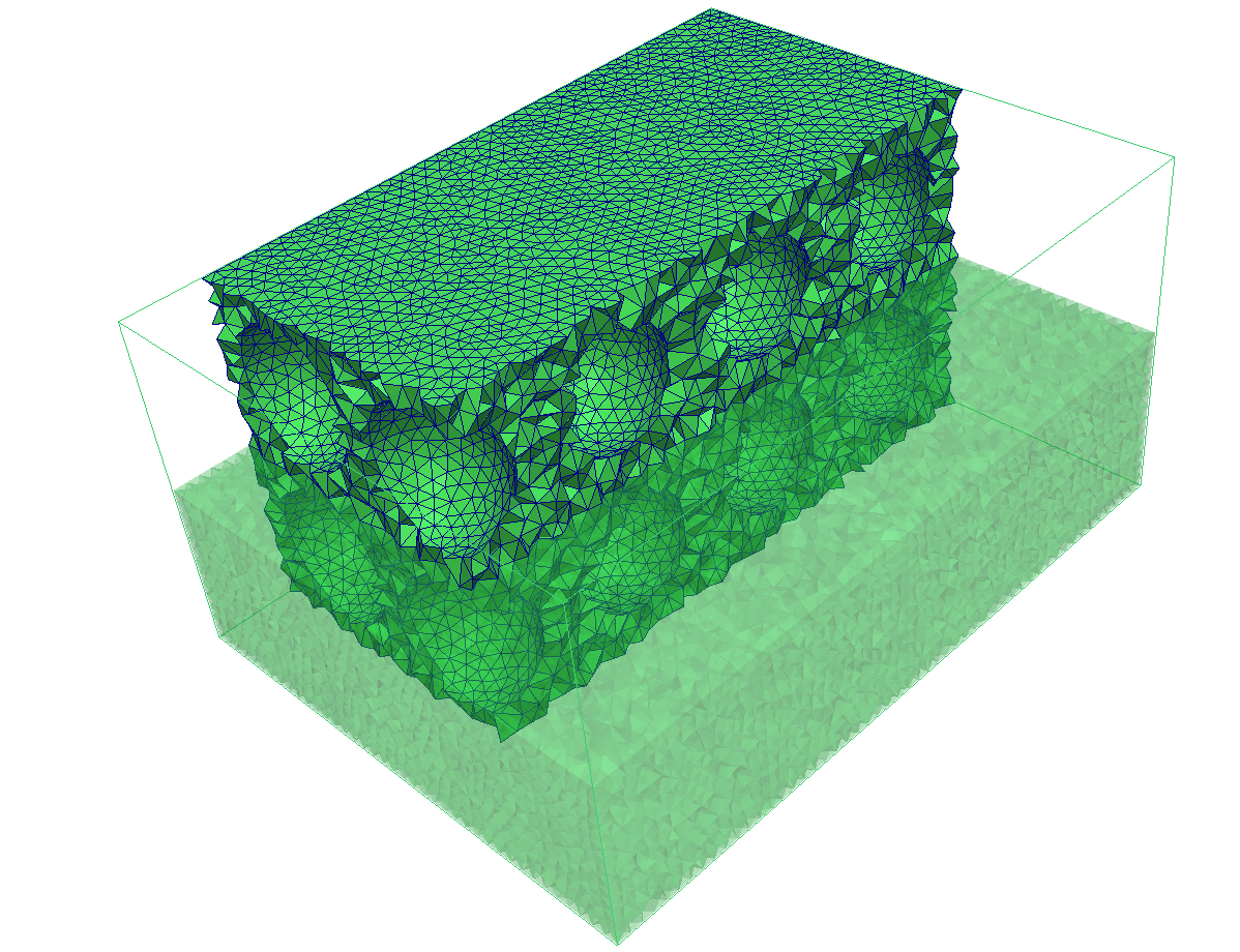
Figure 10: The coarse mesh connectivity that we use for the partition tests motivated by an adapted forest. It consists of $n_{x}\times n_{y}\times n_{z}$ cubes with one spherical hole each. For this picture we use $n_{x}=4,\,n_{y}=3,\,n_{z}=2$, and each cube is triangulated with approximately 7575 tetrahedra. For illustration purposes we show parts of the mesh opaque and other parts are invisible.

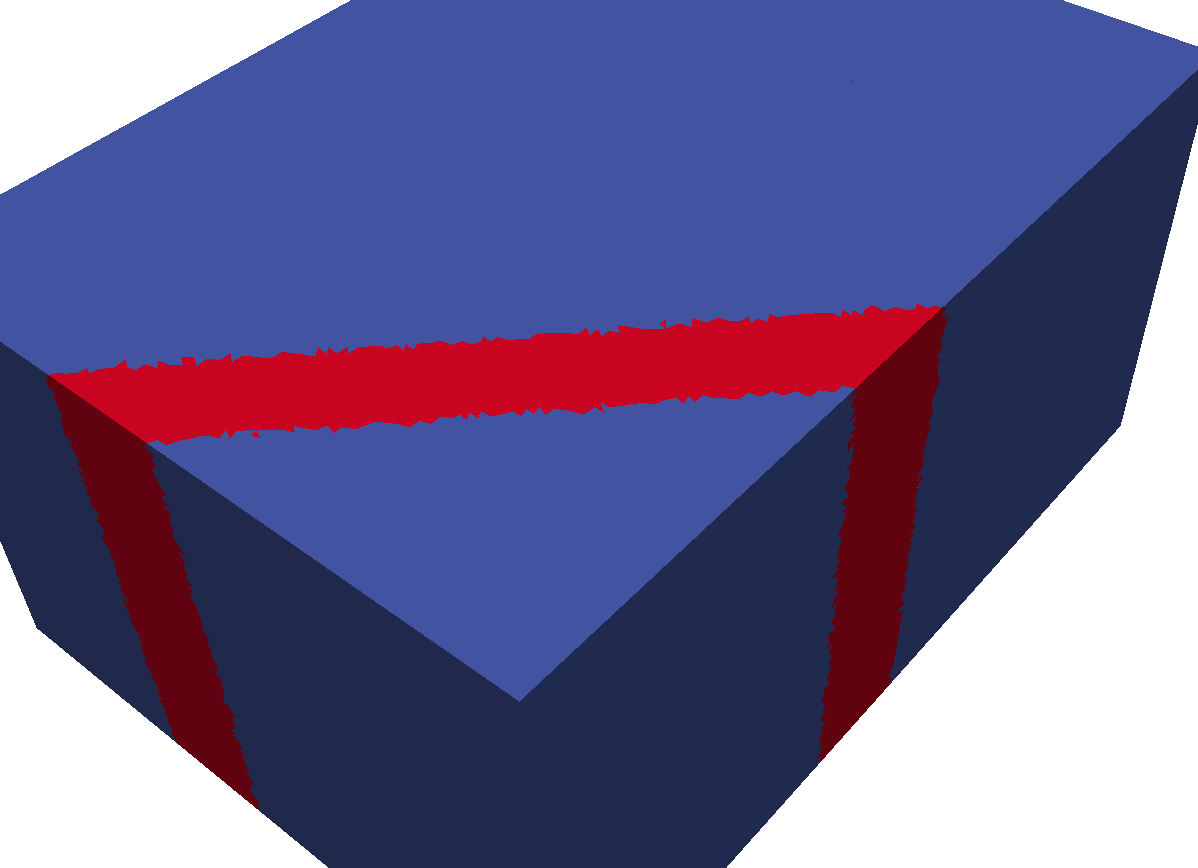
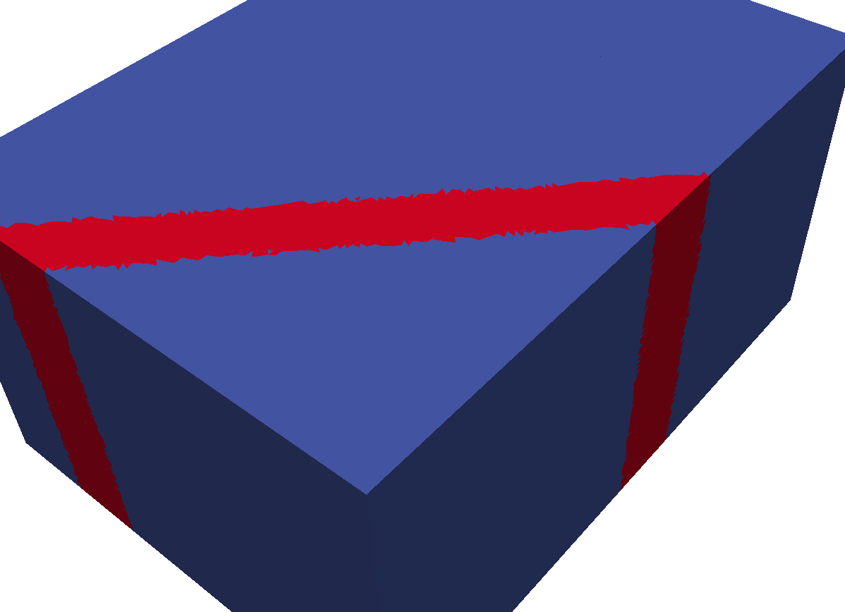
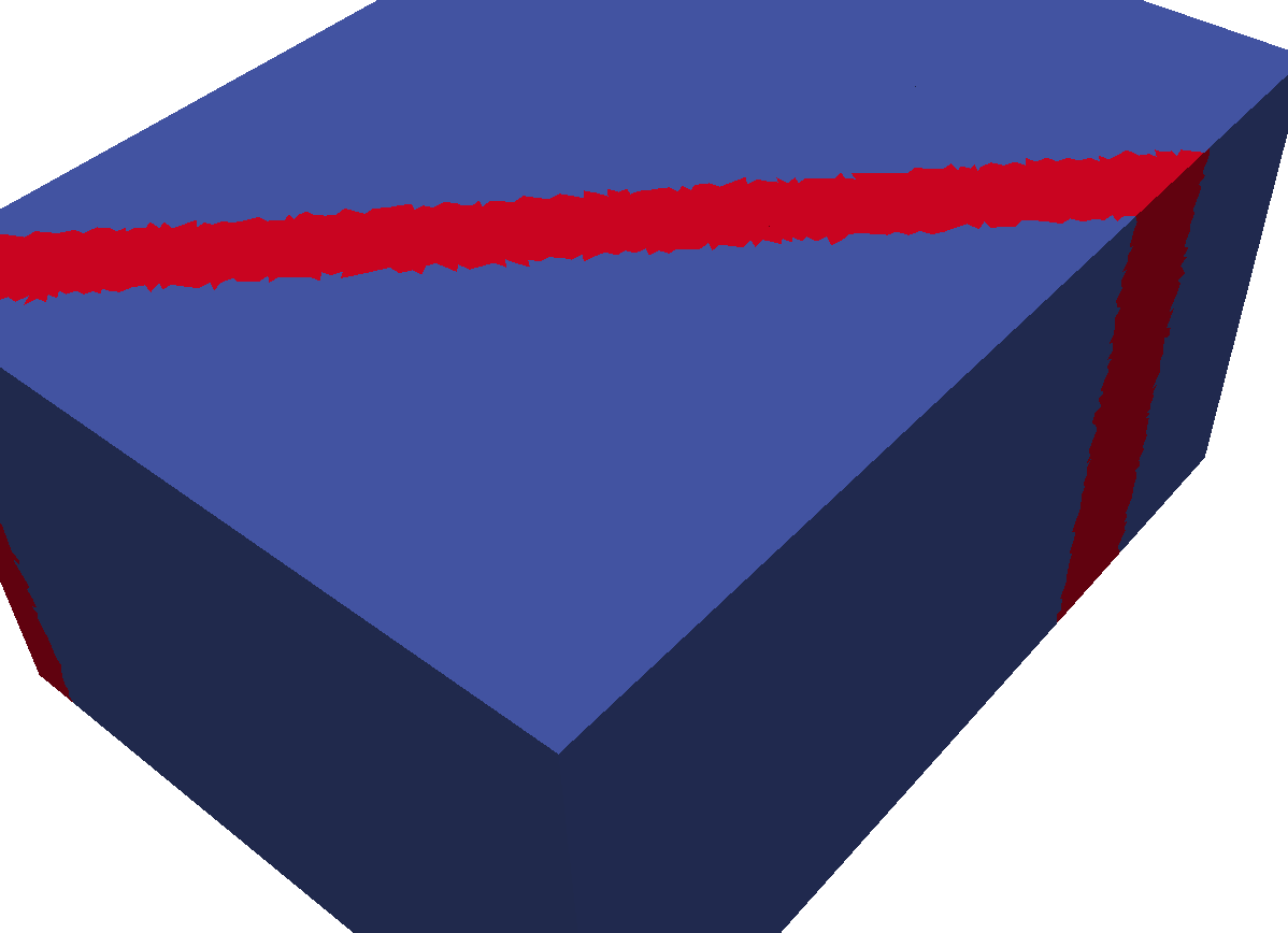
Figure 11: An illustration of the band of finer forest mesh elements in the example. The region of finer mesh elements moves through the mesh in each time step. From left to right we see $t=1$, $t=2$, and $t=3$. In this illustration, elements of refinement level 1 are blue and elements of refinement level 2 are red.

Coarse mesh partition on 8,192 MPI ranks

t	trees (ghosts) sent	data sent [MiB]	$|S_{p}|$	shared trees	run time [s]
1	25,116.7 (11,947.5)	4.945	2.274	7178	0.103
2	34,860.3 (16,854.9)	6.880	2.753	7176	0.110
3	36,386.0 (17,567.6)	7.180	2.823	7182	0.112
1	39,026.2 (18,333.9)	7.670	2.962	8096	0.128
2	38,990.1 (18,268.0)	7.660	2.946	8085	0.129
3	38,941.7 (18,073.9)	7.639	2.933	8085	0.128

Table 3: Partition_cmesh with a coarse mesh of 324,766,336 tetrahedral trees on 8192 MPI ranks. We measure mesh repartition for three time steps. For each we show process average values of the number of trees ghosts, and total number of bytes that each process sends to other processes. The average number of other processes to which a process sends ($|S_{p}|$) is in each test below three. We also give the total number of shared trees in the mesh, 8191 being the maximum possible value. We round all numbers to three significant figures. $1\textrm{ MiB}=1024^{2}\textrm{ bytes}.$

Forest mesh partition on 8,192 MPI ranks

t	mesh size	elements sent	data sent [MiB]	run time [s]
1	2,622,283,453	203,858	3.494	0.215
2	2,623,842,241	281,254	4.824	0.215
3	2,626,216,984	293,387	5.032	0.214
1	25,155,319,545	3,013,230	46.574	0.642
2	25,285,522,233	3,008,800	46.506	0.640
3	25,426,331,342	2,991,990	46.248	0.645

Table 4: For the same example as in Table 3 we display statistics and run times for the forest mesh partition. We show the total number of tetrahedral elements, and the average count of elements and bytes that each process sends to other processes (their count is the same as in Table 3). We round all numbers to three significant figures.

Coarse mesh partition on 458,752 MPI ranks

t	trees (ghosts) sent	data sent [MiB]	$|S_{p}|$	shared trees	run time [s]
1	703.976 (2444.11)	0.267	2.986	280,339	0.207
2	707.368 (2455.95)	0.269	2.996	281,694	0.204
3	707.904 (2457.70)	0.269	2.997	281,900	0.204

Forest mesh partition on 458,752 MPI ranks

t	mesh size	elements sent	data sent [MiB]	run time [s]
1	167,625,595,829	362,863	5.548	0.522
2	167,709,936,554	364,778	5.577	0.578
3	167,841,392,949	365,322	5.585	0.567

Table 5: Run times for coarse mesh and forest partition for the brick with holes on 458,752 MPI ranks. The setting and the coarse mesh are the same as in Table 3 despite that for the forest we use a initial uniform level three refinement with a maximum level of four.

6 Conclusion

In this manuscript we propose an algorithm that executes dynamic and in-core coarse mesh partitioning. In the context of forest-of-trees adaptive mesh refinement, the coarse mesh defines the connectivity of tree roots, which is used in all neighbor query operations between elements. This development is motivated by simulation problems on complex domains that require large input meshes. Without partitioning, we will run out of memory around one million coarse elements, and with static or out-of-core partitioning, we might not have the flexibility to transfer the tree meta data as required by the change in process ownership of the trees’ elements, which occurs in every AMR cycle. With the approach presented here, this can be performed with run times that are significantly smaller than those for partitioning the elements, even considering that SFC methods for the latter are exceptionally fast in absolute terms. Thus, we add little to the run time of all AMR operations combined.

Our algorithm guarantees both, that the number of fine mesh elements is distributed equally among the processes using a space-filling curve, and that each process can provide the necessary connectivity data for each of its fine mesh elements. We handle the communication without handshaking and develop a communication pattern that minimizes data movement. This pattern is calculated by each process individually, reusing information that is already present.

Our implementation scales up to 917e3 MPI processes and up to 810e3 coarse mesh elements per process, where the largest test case consists of .37e12 coarse mesh elements. What remains to be done is extending the partitioning of ghost trees to edge and corner neighbors, since only face neighbor ghost trees are presently handled. It appears that the structure of the algorithm will allow this with little modification.

References

- [1] M. Bader and Ch. Zenger. Efficient Storage and Processing of Adaptive Triangular Grids Using Sierpinski Curves, pages 673–680. Springer, 2006.
- [2] Michael Bader. Space-Filling Curves: An Introduction with Applications in Scientific Computing. Texts in Computational Science and Engineering. Springer, 2012.
- [3] Wolfgang Bangerth, Ralf Hartmann, and Guido Kanschat. deal.II – a general-purpose object-oriented finite element library. ACM Transactions on Mathematical Software, 33(4):24, 2007.
- [4] Marsha J. Berger and Phillip Colella. Local adaptive mesh refinement for shock hydrodynamics. J. Comput. Phys., 82(1):64–84, May 1989.
- [5] Marsha J. Berger and Joseph Oliger. Adaptive mesh refinement for hyperbolic partial differential equations. Journal of Computational Physics, 53(3):484–512, 1984.
- [6] Jürgen Bey. Der BPX-Vorkonditionierer in drei Dimensionen: Gitterverfeinerung, Parallelisierung und Simulation. Universität Heidelberg, 1992. Preprint.
- [7] Greg Bryan. Enzo 2.5 documentation. Laboratory for Computational Astrophysics, University of Illinois, 2016. Last accessed Oct 30, 2016.
- [8] A. Burri, A. Dedner, R. Klöfkorn, and M. Ohlberger. An efficient implementation of an adaptive and parallel grid in DUNE, pages 67–82. Springer, 2006.
- [9] Carsten Burstedde. p4est: Parallel AMR on forests of octrees, 2010. \urlhttp://www.p4est.org/ (last accessed February 27, 2015).
- [10] Carsten Burstedde, Donna Calhoun, Kyle T. Mandli, and Andy R. Terrel. Forestclaw: Hybrid forest-of-octrees AMR for hyperbolic conservation laws. In Michael Bader, Arndt Bode, Hans-Joachim Bungartz, Michael Gerndt, Gerhard R. Joubert, and Frans Peters, editors, Parallel Computing: Accelerating Computational Science and Engineering (CSE), volume 25 of Advances in Parallel Computing, pages 253 – 262. IOS Press, March 2014.
- [11] Carsten Burstedde and Johannes Holke. A tetrahedral space-filling curve for nonconforming adaptive meshes. SIAM Journal on Scientific Computing, 38(5):C471–C503, 2016.
- [12] Carsten Burstedde, Lucas C. Wilcox, and Omar Ghattas. p4est: Scalable algorithms for parallel adaptive mesh refinement on forests of octrees. SIAM Journal on Scientific Computing, 33(3):1103–1133, 2011.
- [13] U.V. Catalyurek, E.G. Boman, K.D. Devine, D. Bozdag, R.T. Heaphy, and L.A. Riesen. Hypergraph-based dynamic load balancing for adaptive scientific computations. In Proc. of 21st International Parallel and Distributed Processing Symposium (IPDPS’07). IEEE, 2007.
- [14] Jülich Supercomputing Centre. JUQUEEN: IBM Blue Gene/Q supercomputer system at the Jülich Supercomputing Centre. Journal of large-scale research facilities, A1, 2015. http://dx.doi.org/10.17815/jlsrf-1-18.
- [15] C. Chevalier and F. Pellegrini. PT-Scotch: A tool for efficient parallel graph ordering. Parallel Computing, 34(6-8):318–331, July 2008.
- [16] T. Coupez, L. Silva, and H. Digonnet. A massivelly parallel multigrid solver using petsc for unstructured meshes on tier0 supercomputer. Presentation at PETSc user meeting, 2016.
- [17] Karen Devine, Erik Boman, Robert Heaphy, Bruce Hendrickson, and Courtenay Vaughan. Zoltan data management services for parallel dynamic applications. Computing in Science and Engineering, 4(2):90–97, 2002.
- [18] Jürgen Dreher and Rainer Grauer. Racoon: A parallel mesh-adaptive framework for hyperbolic conservation laws. Parallel Computing, 31(8):913–932, 2005.
- [19] Christophe Geuzaine and Jean-François Remacle. Gmsh: A 3-d finite element mesh generator with built-in pre- and post-processing facilities. International Journal for Numerical Methods in Engineering, 79(11):1309–1331, 2009.
- [20] M. Griebel and G. Zumbusch. Parallel multigrid in an adaptive PDE solver based on hashing. In E. H. D’Hollander, G. R. Joubert, F. J. Peters, and U. Trottenberg, editors, Parallel Computing: Fundamentals, Applications and New Directions, Proceedings of the Conference ParCo’97, 19–22 September 1997, Bonn, Germany, volume 12, pages 589–600. Elsevier, North-Holland, 1998.
- [21] M. Griebel and G. Zumbusch. Hash based adaptive parallel multilevel methods with space-filling curves. In Horst Rollnik and Dietrich Wolf, editors, NIC Symposium 2001, volume 9 of NIC Series, ISBN 3-00-009055-X, pages 479–492, Germany, 2002. Forschungszentrum Jülich.
- [22] D. Hilbert. Über die stetige Abbildung einer Linie auf ein Flächenstück. Mathematische Annalen, 38:459–460, 1891.
- [23] George Karypis and Vipin Kumar. A parallel algorithm for multilevel graph partitioning and sparse matrix ordering. Journal of Parallel and Distributed Computing, 48:71–95, 1998.
- [24] R.M. Maxwell, S.J. Kollet, S.G. Smith, C.S. Woodward, R.D. Falgout, I.M. Ferguson, N. Engdahl, L.E Condon, B. Hector, S.R. Lopez, J. Gilbert, L. Bearup, J. Jefferson, C. Collins, I. de Graaf, C. Prubilick, C. Baldwin, W.J. Bosl, R. Hornung, and S. Ashby. ParFlow User’s Manual. Integrated Ground Water Modeling Center, Report GWMI 2016-01 edition, 2016.
- [25] Oliver Meister, Kaveh Rahnema, and Michael Bader. Parallel memory-efficient adaptive mesh refinement on structured triangular meshes with billions of grid cells. ACM Trans. Math. Softw., 43(3):19:1–19:27, September 2016.
- [26] G. M. Morton. A computer oriented geodetic data base; and a new technique in file sequencing. Technical report, IBM Ltd., 1966.
- [27] Charles D. Norton, Greg Lyzenga, Jay Parker, and Robert E. Tisdale. Developing parallel GeoFEST(P) using the PYRAMID AMR library. Technical report, Jet Propulsion Laboratory, National Aeronautics and Space Administration, 2004.
- [28] Guiseppe Peano. Sur une courbe, qui remplit toute une aire plane. Math. Ann., 36(1):157–160, 1890.
- [29] Ali Pinar and Cevdet Aykanat. Fast optimal load balancing algorithms for 1D partitioning. Journal on Parallel and Distributed Computing, 64(8):974–996, August 2004.
- [30] Abtin Rahimian, Ilya Lashuk, Shravan Veerapaneni, Aparna Chandramowlishwaran, Dhairya Malhotra, Logan Moon, Rahul Sampath, Aashay Shringarpure, Jeffrey Vetter, Richard Vuduc, et al. Petascale direct numerical simulation of blood flow on 200k cores and heterogeneous architectures. In Proceedings of the 2010 ACM/IEEE International Conference for High Performance Computing, Networking, Storage and Analysis, pages 1–11. IEEE Computer Society, 2010.
- [31] M. Rasquin, C. Smith, K. Chitale, E. S. Seol, B. A. Matthews, J. L. Martin, O. Sahni, R. M. Loy, M. S. Shephard, and K. E. Jansen. Scalable implicit flow solver for realistic wing simulations with flow control. Computing in Science Engineering, 16(6):13–21, Nov 2014.
- [32] Werner C. Rheinboldt and Charles K. Mesztenyi. On a data structure for adaptive finite element mesh refinements. ACM Transactions on Mathematical Software, 6(2):166–187, 1980.
- [33] Hsi-Yu Schive, Yu-Chih Tsai, and Tzihong Chiueh. Gamer: a graphic processing unit accelerated adaptive-mesh-refinement code for astrophysics. The Astrophysical Journal Supplement Series, 186(2):457, 2010.
- [34] P. M. Selwood and M. Berzins. Parallel unstructured tetrahedral mesh adaptation: algorithms, implementation and scalability. Concurrency: Practice and Experience, 11(14):863–884, 1999.
- [35] Jonathan Richard Shewchuk. Triangle: Engineering a 2D quality mesh generator and Delaunay triangulator. In Ming C. Lin and Dinesh Manocha, editors, Applied Computational Geometry: Towards Geometric Engineering, volume 1148 of Lecture Notes in Computer Science, pages 203–222. Springer, 1996. From the First ACM Workshop on Applied Computational Geometry.
- [36] Hang Si. TetGen—A Quality Tetrahedral Mesh Generator and Three-Dimensional Delaunay Triangulator. Weierstrass Institute for Applied Analysis and Stochastics, Berlin, 2006.
- [37] Wacław Sierpiński. Sur une nouvelle courbe continue qui remplit toute une aire plane. Bulletin de l’Académie des Sciences de Cracovie, Séries A:462–478, 1912.
- [38] William Skamarock, Joseph Oliger, and Robert L Street. Adaptive grid refinement for numerical weather prediction. J. Comput. Phys., 80(1):27 – 60, 1989.
- [39] C. W. Smith, M. Rasquin, D. Ibanez, K. E. Jansen, and M. S. Shephard. Application specific mesh partition improvement. Technical Report 2015-3, Rensselaer Polytechnic Institute, 2015.
- [40] David A Steinman, Jaques S Milner, Chris J Norley, Stephen P Lownie, and David W Holdsworth. Image-based computational simulation of flow dynamics in a giant intracranial aneurysm. American Journal of Neuroradiology, 24(4):559–566, 2003.
- [41] James R. Stewart and H. Carter Edwards. A framework approach for developing parallel adaptive multiphysics applications. Finite Elements in Analysis and Design, 40(12):1599–1617, 2004.
- [42] Hari Sundar, Rahul Sampath, and George Biros. Bottom-up construction and 2:1 balance refinement of linear octrees in parallel. SIAM Journal on Scientific Computing, 30(5):2675–2708, 2008.
- [43] Tiankai Tu, David R. O’Hallaron, and Omar Ghattas. Scalable parallel octree meshing for terascale applications. In SC ’05: Proceedings of the International Conference for High Performance Computing, Networking, Storage, and Analysis. ACM/IEEE, 2005.
- [44] Tobias Weinzierl and Miriam Mehl. Peano—a traversal and storage scheme for octree-like adaptive Cartesian multiscale grids. SIAM Journal on Scientific Computing, 33(5):2732–2760, October 2011.
- [45] Yusuf Yılmaz, Can Özturan, Oğuz Tosun, Ali Haydar Özer, and Seren Soner. Parallel mesh generation, migration and partitioning for the elmer application. Technical report, PREMA-Partnership for Advanced Computing in Europe, 2010.
- [46] M. Zhou, O. Sahni, K. D. Devine, M. S. Shephard, and K. E. Jansen. Controlling unstructured mesh partitions for massively parallel simulations. SIAM Journal on Scientific Computing, 32(6):3201–3227, 2010.
- [47] G. Zumbusch. Parallel Multilevel Methods. Adaptive Mesh Refinement and Load Balancing. Teubner, 2003.