Colorings of odd or even chirality on hexagonal lattices

Abstract

We define two classes of colorings that have odd or even chirality on hexagonal lattices. This parity is an invariant in the dynamics of all loops, and explains why standard Monte-Carlo algorithms are nonergodic. We argue that adding the motion of “stranded” loops allows for parity changes. By implementing this algorithm, we show that the even and odd classes have the same entropy. In general, they do not have the same number of states, except for the special geometry of long strips, where a Z₂ symmetry between even and odd states occurs in the thermodynamic limit.

I Introduction

Constructing classical states that satisfy some local constraints everywhere on a lattice may be a difficult problem. The simplest physical examples of such problems include dimer coverings of lattices, perfect tilings of a surface with tiles of special geometry, coloring sites with distinct colors, folding paper (origami). They have in common that they can be formulated with ice-type or vertex models. The calculation of the number of states and the thermodynamics is difficult, but has been solved exactly in some cases. There are also interesting issues regarding conservation laws in the dynamics and hidden higher symmetries.

A way to construct numerically such constrained states is to iterate a dynamical process, starting from a simple state. In particular, classical Monte-Carlo algorithms sample the ensemble of states by flipping variables collectively in order to preserve the constraints,Newman either along loopsStillinger or in clusters of sites.Wang There are now examples of models where such algorithms are nonergodic, and conservation laws may hinder classes of states. This is the case of some dimer models on lattices in three spatial dimensions, where the nonergodicity is restricted to flipping the smallest loops.Sikora ; Freedman This is also generically the case when periodic boundary conditions create sectors characterized by winding numbers: here again the ergodicity is simply restored by including in the dynamics the loops that wind accross the boundaries.

A different example is given by the three-color Baxter’s modelBaxter that we will consider here. In this model, the constraint consists of coloring the edges of a regular hexagonal lattice with three colors such that no two neighbors have the same color. Baxter calculated exactly the entropy of the three-colorings for a hexagonal lattice with open boundary conditions. In order to compute some observables, loop Monte-Carlo algorithms have been set up but it has been recognized that they are nonergodic for lattices with periodic boundary conditions,Huse ; Mohar possibly leading to systematic errors. In particular, some states that are not connected by the dynamics, have been constructed on finite-size systems, leading to the conclusion that there are more than one class of states.Mohar Since this property is intimately related to the topology of the two-dimensional lattice, an alternative Monte-Carlo approachMoore is to use other geometries for the boundaries, such as a plane with open boundary conditions (but it suffers from more finite-size effects) or a “projective plane”, although the hexagonal lattice has some noncubic vertices in this case.

Restricting to standard periodic boundary conditions and studying why this dynamics in particular is nonergodic is nevertheless interesting, as a point of principle. This dynamics is not only used in Monte-Carlo algorithms but also in quantum models constructed from these constrained states (see Refs. Castelnovo, ; Cepas, in the coloring context). Nonergodicity is generally related to some conservation laws (or broken symmetries) which may have some consequences in various problems. It is also used in applications, e.g. as bits, and some proposals emphasized the advantage of the topological nature of the ergodicity breaking in dimer models.Ioffe Even though imposing periodic boundary conditions seems to be an “academic” problem -they are not that of crystals-, it is, in principle, possible to (i) design artificial superconducting or magnetic devices with special geometry of the boundaries,realpbc (ii) consider molecular nanomagnets that realize special topologies, e.g. a sphere or a ring in the “keplerate” family.keplerate Another close model is the three-coloring model with an additional achiral constraint on the states which generates an infinite number of sectors, even when winding loops are allowed to flip.Fendley ; Korshunov

In the absence of ergodic algorithms to construct all states, simple properties such as the number of missed states are not known. Is this number extensive with the system size or not? If it is, what is the entropy of the new class? Given a state, how do we know whether it is connected to a simple reference state of a given class, i.e. what is the reason of the obstruction to ergodicity? Can we construct an ergodic algorithm that will visit all states? We answer these questions in the present paper.

The paper is organized as follows. We define the model in section II, and we construct all three-coloring states on small clusters in section III.1, from dimer coverings. We check the numbers of three-colorings by using the method of transfer matrix in section III.2. In section IV, we study the dynamics of loops. In addition to standard winding-number classes which we recall (IV.1), we find some other invariant classes under the winding loops (IV.2). We identify a conserved quantity which is the parity of the total chirality (IV.2.1) and briefly discuss some other sectors (IV.2.2 and IV.2.3). We then enumerate separatly odd and even states by appropriate transfer matrices, which allow to extract entropies of infinitely-long strips (section V). We introduce a Monte-Carlo dynamics that does not conserve the parity in section VI.1, and compute the fraction of odd states extrapolated to the thermodynamic limit and the order-parameter in section VI.2. In appendix A, in order to check the construction of section III.1, we recall the method of Pfaffians to enumerate dimer coverings, and give the actual numbers of configurations. It also allows to discuss a general invariant of dimer coverings (appendix B), which in turn is useful to define another formulation of the parity (appendix C). The appendix D treats the same problem where the toroidal boundary condition is replaced by a Klein bottle geometry, leading to similar conclusions.

II Model

We consider the model of color variables $\sigma_{i}=A,B,C$ defined on the edges $i=1,\dots,N$ of a regular honeycomb lattice (sites of the kagome lattice) with periodic boundary conditions. The three edges meeting at each vertex must be in different colors: this local constraint defines the 3-color Baxter’s model.Baxter Each state is referred as a “3-coloring” of the lattice. The number of valid configurations, i.e. respecting the constraints everywhere scales as $\exp(Ns_{\infty})$ in the thermodynamic limit ($s_{\infty}=0.126375...$).Baxter

In the following, the model is defined on finite-size clusters with two different shapes, the rhombus (R) and hexagonal (H) shapes shown in Figs. 1 and 2. We also consider two different boundary conditions, realizing the topology of the “torus” (see the arrows in Fig. 1) or of the “Klein bottle” (appendix D). Both surfaces have zero Euler characteristic and regular hexagonal lattices fit without introducing noncubic vertices.

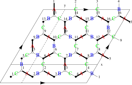
Figure 1: Hexagonal lattice with rhombus shape (R) and periodic boundary conditions of the torus geometry. A dimer and color configurations are shown. Here $L=M=4$ and $N=3\times L\times M=48$ edges. The honeycomb lattice is bipartite and is divided in $L\times M$ black and $L\times M$ white sites. The solid and dashed line show two distinct nonlocal cuts that define topological conserved numbers.

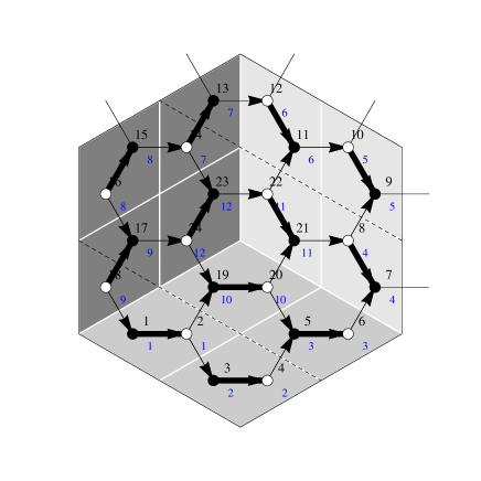
Figure 2: Hexagonal lattice with hexagonal shape (H), here $L=2$ and $N=9L^{2}=36$ edges ($N_{v}=6L^{2}$). A special dimer configuration is shown, sometimes called the “empty room” state in the context of tilings an hexagon with lozenges: the gray colors of the lozenges correspond to the dimer orientations and can be seen as the three walls of an $L^{3}$ “empty room”. The dashed line shows one nonlocal cut accross the boundaries.

III Exact construction and enumeration of 3-colorings on small lattices

III.1 Exhaustive construction

The exhaustive construction of states satisfying the constraints everywhere is possible numerically only on very small clusters, since the number of states increases exponentially with the system size. For this, we first construct the dimer coverings of the lattice by filling an empty lattice with dimers, and checking the constraints at each step.methodenum Once a dimer covering is obtained, each vertex has one edge (out of three) occupied by a dimer -this edge is called color A. The other two edges form a closed loop of even length (on the clusters with periodic boundary conditions we have considered), which is filled with B and C (or C and B) alternatively (see Fig.1 for an example). The dimer configuration has $n_{D}$ such nonintersecting closed loops, which define $2^{n_{D}}$ colorings. Note that we obtain all 3-colorings in this way since any of them can explicitly be decomposed in a dimer configuration (the A colors) plus a loop configuration. It is numerically more efficient than enforcing the color constraint on every vertex. By constructing all dimer coverings, we compute the partition function,

$$Z=\sum_{D}1,$$ (1)

and the number of three-colorings,

$$Z_{3}=\sum_{D}2^{n_{D}},$$ (2)

where $n_{D}$ is the number of loops of the dimer configuration $D$. In this form, $Z_{3}$ is also the partition function of the O(2) fully packed loop model on the honeycomb lattice. The table 1 gives the numbers $Z$ and $Z_{3}$ for the torus boundary conditions, obtained by the explicit construction of individual states as explained above. $Z_{3}$ is a multiple of six, since the six color permutations of the first edge are equivalent, while $Z$ is a multiple of three only for the torus, where the three edge directions are equivalent. As a first check, the entropy per site for $N=192$, $\frac{1}{N}\log Z_{3}=0.1326$, differs from Baxter’s thermodynamic limit, $0.126375$,Baxter by a typical $1/N$ correction, as expected. In order to check these numbers more carefully, we have calculated $Z$ exactly on finite-size systems by using the method of Pfaffians (details are given in appendix A). While no closed form is known for $Z_{3}$ on finite-size systems and the method of Pfaffians is not applicable, we have used a numerical transfer matrix method that we explain now.

$N$	L	T	$Z$	$Z_{3}$
9	1	H	6	12
36	2	H	120	504
81	3	H	15,162	135,552
144	4	H	13,219,200	358,453,104
12	2	R	9	24
27	3	R	42	120
48	4	R	417	2,160
75	5	R	7,623	49,416
108	6	R	263,640	3,226,032
147	7	R	17,886,144	475,299,936
192	8	R	2,249,215,617	113,902,581,984

Table 1: Number of dimer coverings, $Z$, and 3-colorings, $Z_{3}$, for system size $N$ (linear size $L=M$) and periodic boundary conditions of the “torus” geometry. R/H stands for rhombus/hexagonal shapes shown in Figs. 1 and 2. $Z$ is also calculated from Pfaffians in appendix A.2 and A.3, $Z_{3}$ from transfer matrix in table 2 for the rhombus geometry.

III.2 Enumeration of $Z_{3}$ by transfer matrix

We have used the transfer matrix method to compute the number of 3-colorings on finite-size systems and check the numbers given above. For this, we define the state of a horizontal row of $L$ vertical edges (see Fig. 1), by $\sigma=(\sigma_{1},\cdots,\sigma_{L})$ where $\sigma_{i}=A,B,C$. We consider two successive rows in the $y$ direction, that we denote by $\sigma$ and $\sigma^{\prime}$ and define a $3^{L}\times 3^{L}$ transfer matrix $T$ by

$$T_{\sigma\sigma^{\prime}}=\sum_{\alpha|\sigma\sigma^{\prime}}1$$ (3)

where the sum is over all possible configurations $\alpha$ of the intermediate set of zig-zag edges compatible with the lower and upper rows $\sigma$ and $\sigma^{\prime}$.

The partition function reads

$$Z_{3}=\sum_{\sigma_{1}}\dots\sum_{\sigma_{M}}T_{\sigma_{1}\sigma_{2}}T_{\sigma_{2}\sigma_{3}}\cdots T_{\sigma_{M}\sigma_{1}}=\mbox{Tr}[T^{M}]$$ (4)

where $M$ is the vertical linear size ($N=3\times L\times M$), and periodic boundary conditions of the torus geometry have been used. Numerically, to obtain the exact integer number of configurations without rounding errors, we perform the $M$ multiplications of matrices and compute the trace.multvsdiag Alternatively, we also diagonalize the transfer matrix and we have,

$$Z_{3}=\mbox{Tr}[T^{M}]=\sum_{i=1}^{3^{L}}\Lambda_{i}^{M}$$ (5)

where $\Lambda_{i=1,\dots,3^{L}}$ are the (complex) eigenvalues of the transfer matrix. The diagonalisation method is faster but we have to round $Z_{3}$ to the nearest integer, which works up to $10^{16}$ configurations, i.e. one over the machine precision. This is less than working with integers but we may compute real quantities for much larger system sizes in the second case.

The total number of edges $N_{i}^{x}$ of color $i=A,B,C$ in the row $\sigma$ is the same in the row $\sigma^{\prime}$; this gives two independent charges $N_{A}^{x}$ and $N_{B}^{x}$ (see also section IV).Baxter The transfer matrix then factorizes in smaller sectors with dimensions $C_{L}^{N_{A}^{x}}C_{L-N_{A}^{x}}^{N_{B}^{x}}$. For the largest sector with $N_{i}^{x}=(\frac{L}{3},\frac{L}{3},\frac{L}{3})$ ($L$ a multiple of three), the dimension typically scales as $L!/(\frac{L}{3}!)^{3}\sim 3^{L}/L$. For $L=12$, the largest dimension is $C_{12}^{4}C_{8}^{4}=34650$, so that we can compute all eigenvalues. We also use permutation symmetries to avoid computing symmetry related sectors by restricting to $N_{A}^{x}\leq N_{B}^{x}\leq N_{C}^{x}$ and applying a multiplicity factor.

The numbers of three-colorings $Z_{3}$ are given for different $L,M$ in table 2 and match those obtained by the exhaustive construction, given in table 1.

$L$	$M$	$Z_{3}$	$Z_{3}^{-}$
2	2	24	0
3	2	48	0
3	3	120	60
4	2	96	0
4	3	408	0
4	4	2160	1920
5	2	192	0
5	3	1284	294
5	4	8208	960
5	5	49416	14076
6	2	384	0
6	3	4752	0
6	4	36096	17280
6	5	317352	78120
6	6	3226032	346176
7	2	768	0
7	3	17412	1158
7	4	185184	143808
7	5	1946964	583014
7	6	30749232	4890312
7	7	475299936	424616016
8	2	1536	0
8	3	68088	0
8	4	916032	139776
8	5	12153168	5007360
8	6	317511600	45634752
8	7	6258486288	1333287648
8	8	113902581984	54363353088
9	2	3072	0
9	3	266232	4596
9	4	4285632	3082752
9	5	80964996	31696566
9	6	3384078480	176330736
9	7	87113393160	33997363116
9	8	2513986458816	719824701888
9	9	84049269591720	5365286483676
10	2	6144	0
10	3	1058808	0
10	4	20484096	10229760
10	5	529208112	198732000
10	6	35145601224	2194614720
10	7	1338325873128	1081718221080
10	8	50904839729376	14465622318720
10	9	2411622439855752	463649604519600
10	10	111152775037945584	95192069243340960

Table 2: Number of 3-colorings, $Z_{3}$, computed by numerical transfer matrix, for rhombi of size $N=3\times L\times M$ and periodic boundary conditions (Fig. 1). $Z_{3}^{-}$ is the number of odd colorings, from section V.

IV Dynamics and conservation laws

The simplest collective dynamics consists of exchanging colors along loops of sites of two colors (they are closed loops when periodic boundary conditions are employed). It is the simplest way to preserve the constraints (note that a single spin flip would not). This collective dynamics is also that defined in Monte-Carlo algorithmsHuse ; Moore ; Chandra ; Chakraborty ; CastelnovoMC ; Chern and quantum three-coloring models.Castelnovo ; Cepas It is known to be nonergodic even when all loops are flipped.Huse ; Mohar ; Moore A different point is that it is also strongly nonergodic (with an exponential number of sectors) when only the small loops are flipped.Cepasq

Since we have constructed all possible states, we now study why the dynamics of all loops is nonergodic. We probe whether two states are connected by the loop dynamics or not. For this, we start from a single state in the ensemble constructed in section III.1 and flip all of its $n_{l}$ loops (winding and nonwinding), giving $n_{l}$ possible new states. We iterate this procedure until no new state is created (see [technical, ] for technical details). If some states in the ensemble have not been reached, we then take a new state and reiterate the same process. When no new state is available in the ensemble, we are sure that we have constructed all classes of states, closed under this dynamics.

IV.1 Winding-number sectors

The dynamics of nonwinding loops conserves some topological numbers. In the present model, they are obtained by defining three cuts oriented at 120 degrees, that cut the edges at 90 degrees and go through the centers of the hexagons (see the first two $x$ and $y$ cuts in Fig. 1). Counting the number of colors along those cuts is a conserved quantity since any nonwinding loop intersects twice the cuts in locations where the colors are different.Castelnovo Flipping a loop exchanges the two colors: this gives nine conserved numbers $N_{i}^{\alpha}=0,\dots,n^{\alpha}$, $i=A,B,C$, $\alpha=x,y,z$ with some constraints. We have indeed

$$N_{A}^{\alpha}+N_{B}^{\alpha}+N_{C}^{\alpha}=n^{\alpha}$$ (6)

where $n^{\alpha}$ is the number of sites along the cut $\alpha$. For example, when $L=M$, we have $n^{\alpha}=L$ for the rhombus shape (Fig. 1), $n^{\alpha}=3L$ for the hexagonal shape with torus geometry (Fig. 2). So that for each $\alpha$, only two out of three are independent. The second constraint comes from the conservation of these numbers from row to row. Consider the square form $L=M$ for instance. We have,

$$L(N_{i}^{x}+N_{i}^{y}+N_{i}^{z})=\frac{N}{3},$$ (7)

because the sum over $x,y,z$ can be seen as a sum over the three sublattices and $N/3$ is the total number of sites with color $i$. This leads to $\sum_{\alpha}N_{i}^{\alpha}=L$ or $3L$, depending on the shape. This constraints the third direction to be determined from the first two. Therefore, only four of the nine $N_{i}^{\alpha}$ are independent. But to emphasize the symmetries it is convenient to write a general configuration of a topological sector by $N_{i}^{\alpha}=(a_{x},b_{x},c_{x},a_{y},b_{y},c_{y},a_{z},b_{z},c_{z})$. Since the number of colors is always positive, we also have inequalities such as $N_{A}^{\alpha}+N_{B}^{\alpha}\leq n$ (for $L=M$) which further reduces the number of possibilities to $(\sum_{k=1}^{n+1}k)^{2}=[(n+1)(n+2)/2]^{2}$. Some of them are not allowed however, so the number of sectors is strictly less that that.

IV.2 Kempe sectors and odd/even classes

When winding loops are added in the dynamics, the winding numbers are no longer conserved and topological sectors are a priori connected. In fact, we find some disconnected classes, sometimes called “Kempe” classes in the literature.Mohar ; Belcastro The number of classes we find is given by $n_{K}$ in table 3, up to some degeneracies that we indicate and discuss in section IV.2.2. $n_{K}$ depends on the geometry and it increases with the system size. Given the limitation in sizes, it is an open question as to whether it is infinite in the thermodynamic limit.

$N$	$n_{K}$	$Z_{i=1,\cdots,n_{K}}(\pm)$
9	2	6(+), 6(-)
36	2	360(+), 144(-)
81	3	111,840(+), 60(-), 23,652(-)
144	5	315,051,888(+), 42,953,088(-), 44,928(x6)(-), 155,520(-), 23,040(-)
12	1	24 (+)
27	2	60(+), 60(-)
48	2	240(+), 1,920(-)
75	3	35,340(+), 276(-), 13,800(-)
108	3	2,879,856(+), 307,296(-), 19,440(x2)(-)
147	4	50,683,920(+), 1140(-), 424,598,328(-), 6 (x2758)(-)
192	4	59,539,228,896(+), 54,178,583,040(-), 14,555,136(-), 28,369,152(x6)(-)

Table 3: Number of invariant classes $n_{K}$ and number of states in each class $Z_{i=1,\dots,n_{K}}$ ($\sum_{i=1}^{n_{K}}n_{i}Z_{i}=Z_{3}$, where $n_{i}$ is the sector multiplicity, given in brackets). The even/odd chirality of each class is given by $\pm$.

Each Kempe sector contains several winding sectors connected by the motion of the winding loops. In the torus geometry, distinct Kempe sectors (we call “distinct” two sectors that are not related by the loop motion but also by a lattice symmetry) contain distinct winding sectors, but this is not true in the Klein bottle geometry.192

The number of states in each sector is given by $Z_{i}$ with $i=1,\dots,n_{K}$ and varies from $Z_{i}\lesssim Z_{3}$ down to $Z_{i}=6$ states. This reflects the topological sectors themselves, which are expected to have Gaussian distribution.Chakraborty

We now show that we can distinguish some of these sectors by the parity of the chirality and some lattice symmetries.

IV.2.1 Conservation law : odd/even chirality

We define the total chirality of a state by,

$$m=\sum_{v}\chi_{v},$$ (8)

where $\chi_{v}=\pm 1/2$ for an ABC (or ACB) orientation of the edges by turning clockwise around any vertex $v$ (Fig. 3). The sum is over all (black and white) $2N/3$ vertices of the bipartite honeycomb lattice. Since the total number of vertices is even, $m$ is an integer that can be even or odd.

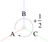
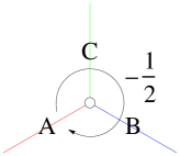
Figure 3: Definition of the chirality at a given (white) vertex (the definition is the same for black vertices). The sum of the chirality of all vertices (black and white) can be even or odd and its parity is conserved.

First, the system always has the chiral symmetry between $m$ and $-m$, obtained by exchanging all A and B, which can be done by moving all A-B loops. Second, nonwinding loops have zero chirality so that $m$ is conserved under the dynamics of nonwinding loops. Third, there may be a finite chirality along a winding loop, $m_{l}$ where $l$ is the length of the loop, which is always even. Flipping this loop reverses the chirality of all its vertices, so $m_{l}\rightarrow-m_{l}$. Since $l$ is even, $m_{l}$ is an integer, and the total chirality changes by $2m_{l}$ which is an even integer, so that the parity of $m$,

$$I_{3}=(-1)^{m},$$ (9)

is conserved in the dynamics of all loops. This defines two odd/even classes and we have labelled the Kempe sectors by this parity in table 3. Note that the odd class is further split into sectors, some of which we will discuss below. Note also that on clusters with open boundary conditions (cylinder or plane), there are open loops at the boundaries that change the chirality of an odd number of vertices, and thus do not conserve the parity.

We give two concrete examples of states with odd or even chirality. We consider first a periodic state with a tripled unit-cell (called $\sqrt{3}\times\sqrt{3}$), obtained by stacking A-B-C along any of the three lattice directions. While it is always compatible with the hexagonal shape, $L$ and $M$ have to be multiples of three on the rhombus shape and it does not fit in the Klein bottle geometry. For this state, the total chirality is zero, always even. For the “$Q=0$” state, all (black and white) vertices have the same configuration, say ABC, so that $m=N/3$. For the square shape with $L=M$, $m$ has the parity of $L$. Therefore for $L$ odd and multiple of three (so as to fit the $\sqrt{3}\times\sqrt{3}$) we have at least two independent sectors. The conclusion $n_{K}>1$ was already reached in Ref. Mohar, and extended for even $L$.

We describe in the appendix C some other formulations of the same invariant.

IV.2.2 Lattice symmetries

We find some degenerate sectors with an identical number of states (table 3). This degeneracy can be explained by lattice symmetries.

Permutation of colors can be implemented by a loop motion, so that two topological sectors related by permutation symmetry, e.g. $(a_{x},b_{x},c_{x},a_{y},b_{y},c_{y},a_{z},b_{z},c_{z})$ and $(b_{x},a_{x},c_{x},b_{y},a_{y},c_{y},b_{z},a_{z},c_{z})$ belong to the same Kempe sector. Permutations generate at most six sectors.

Applying lattice symmetries is a different operation that generates other sectors that may not be connected by the dynamics. For instance, applying a $x-y$ mirror plane gives $(a_{y},b_{y},c_{y},a_{x},b_{x},c_{x},a_{z},b_{z},c_{z})$. Successive applications of the three mirror planes generates at most six sectors if all the charges are different.

For instance, for $N=108$, there are two Kempe sectors with 19440 states. They are related by a mirror symmetry. Indeed the winding sectors in one of these two Kempe classe have the special form $(a,b,c,b,c,a,c,a,b)$ (up to color permutations), and $(b,c,a,a,b,c,c,a,b)$ in the other. Mirror symmetries up to permutations generate only two sectors in this case. However, for $N=144$ or $N=192$, there is a six-fold degeneracy that is obtained by using the three mirror planes.

These degeneracies are robust in that any local perturbation that breaks the mirror symmetry has the same average in both sectors, as expected for topological sectors.Ioffe

IV.2.3 Special sectors

Some sectors have no weight in the thermodynamic limit.

A first example is the sector of the “$Q=0$” state, when $L$ is odd. This state belongs to the smallest nondegenerate sector (see table 3). It has maximal chirality with all vertices in the $\pm$ state, $m=\pm N/3$. Since $m$ is a multiple of $L$, and all winding loop lengths are multiples of $2L$, the chirality changes by $2L$ and remains therefore a multiple of $L$. The new winding loops have lengths that remain multiples of $2L$ so that the Kempe sector has $m=\pm(1+2n)L$ which is not only odd but is also a multiple of $L$, a property that remains stable in the dynamics.

A second example is found for $N=147$. We find 2758 degenerate sectors containing only 6 states. Some of these sectors are related by translation symmetry but are special in that they minimize the number of loops, i.e. three. Each loop, say the A-B one, takes all the $N/3$ A edges and the $N/3$ B edges. This loop connects all sites of the honeycomb lattice and is an Hamiltonian cycle. Flipping an A-B loop exchanges the A-C and B-C loops and therefore keeps the lengths identical. Such a structure is therefore stable and has only six states obtained by the only six possible permutations. We have not found this structure on the other clusters available, but it may exist for larger sizes. Note that while there is always a Hamiltonian path on a regular honeycomb lattice, this is not always true for such three intertwined Hamiltonian paths.

V Enumeration of odd/even states by transfer matrix

We compute the number of odd/even states by introducing a modified partition function, $P(z)$ with a fugacity $z$,

$$P(z)=\sum_{C}z^{m}$$ (10)

where the sum is over all 3-color configurations and $m$ is the total chirality of the configuration $C$, defined in section IV.2.1. The total number of colorings is

$$Z_{3}=P(1).$$ (11)

However, $z$ in Eq. 10 can be any number. Given that, by symmetry, there is the same number of states with $m$ and $-m$, we have $P(1/z)=P(z)$. In particular, we consider $P(z)$ with $z=-1$, which contains terms of the form $(-1)^{m}=\pm 1$. These terms differ by their signs in the two parity sectors (IV.2.1), therefore all even colorings are counted with a $+$ sign while odd colorings are counted with a $-$ sign. We obtain the number of odd colorings by

$$Z_{3}^{-}=\frac{1}{2}[P(1)-P(-1)].$$ (12)

and the number of even colorings, from $Z_{3}=Z_{3}^{+}+Z_{3}^{-}$. To compute this number, we construct a transfer matrix with elements,

$$T_{\sigma\sigma^{{}^{\prime}}}(z)=\sum_{\alpha|\sigma\sigma^{{}^{\prime}}}z^{m},$$ (13)

where the sum is over the configurations $\alpha$ of the intermediate zig-zag row compatible with the pair of rows $\sigma$ and $\sigma^{\prime}$, and $m$ is the partial chirality of that row. We restrict the fugacity to $z=-1$, so that the transfer matrix has integer entries. The number of configurations $Z_{3}^{-}$ is then computed as an integer by matrix multiplications, from

$$P(\pm 1)=\mbox{Tr}[T(\pm 1)^{M}],$$ (14)

and Eq. 12. The results are given in table 2 and they match the numbers found by the dynamical process (table 3).

V.1 Rotation symmetry

We note that the transfer matrix $T(-1)$ has an exact SU(3) symmetry even on finite size systems, since we have explicitly checked that

$$[T(-1),\sum_{i=1}^{L}\lambda_{c}(i)]=0$$ (15)

for all the $c=1,\dots,8$ generators of SU(3), $\lambda_{c}(i)$ on edge $i$. A consequence is that the eigenvalues of $T(-1)$ have degeneracies that are that of the multiplets of SU(3). In this language, the conserved isospin and hypercharge are obtained from the number of colors, by $T_{3}=\frac{1}{2}(N_{A}^{x}-N_{B}^{x})$ and $Y=\frac{1}{3}(N_{A}^{x}+N_{B}^{x}-2N_{C}^{x})$.

Fig. 4 gives an example of the eigenvalues of $T(-1)$ for $L=5$, in the complex plane. We find that they form multiplets belonging to the following irreducible representations of SU(3), $5\times[3]+6\times[6]+5\times[\bar{15}]+[21]+4\times[24]\equiv 3^{5}$, where the number in bracket gives the dimension of the representation, the bar specifies the right of left representation and the number in front the number of such multiplets. Some additional degeneracies are found, such as $[24]$ and $[\bar{15}]$, or $[21]$ and $[\bar{15}]$, which seem to be accidental but may indicate a higher symmetry than SU(3).

This symmetry enhancement at a critical point ($z=-1$), is very similar to a spin-ice model where an exact SU(2) symmetry was found in finite-size systems.Jaubert It was also conjectured that the SU(3) symmetry holds for $z=1$ but only in the thermodynamic limit.Read ; Kondev

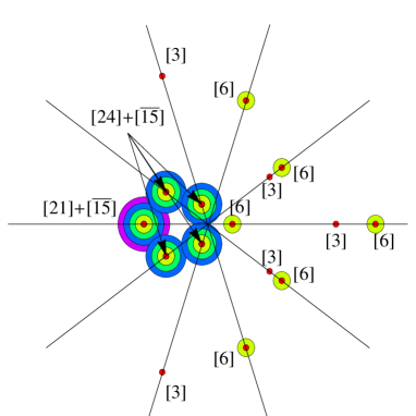
Figure 4: Eigenvalues of the transfer matrix $T(-1)$ (given here in the complex plane for $L=5$) are degenerate and form the multiplets of SU(3), $[3],[6],[\bar{15}],[21],[24]$. The colors indicate different charge sectors (the degeneracy due to permutation-related sectors is not shown).

V.2 Fraction of odd states

We compute the exact fraction of odd states for finite-size $L$, as a real number, from the complete diagonalisation of the transfer matrices,

$$\frac{Z_{3}^{-}}{Z_{3}}=\frac{1}{2}\left[1-\frac{P(-1)}{P(1)}\right]$$ (16)

The result is given in Fig. 5 as a function of $M$, for different $L$ up to $L=12$.

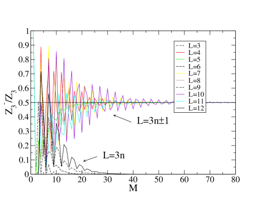
Figure 5: Fraction of odd states as a function of $M$ for a strip of size $N=3\times L\times M$ with rhombus shape and periodic boundary conditions, from transfer matrix. When $M\rightarrow\infty$, the fraction goes to 0 for $L=3n$ and 1/2 for $L=3n\pm 1$, thus exhibiting a $Z_{2}$ symmetry between even and odd states.

We can study the limit of large transverse size $M\rightarrow+\infty$, i.e. a thermodynamic limit with zero aspect ratio $r=L/M\rightarrow 0$. In this case, we are interested in the largest eigenvalues, and we have to distinguish two cases, depending on whether $L$ is a multiple of three or not.

V.2.1 $L=3n$ ($L$ a multiple of three)

In this case, we find that the largest eigenvalue of $T(1)$, $\Lambda_{1}$ equals that of $T(-1)$, $\Lambda_{1}^{-}$ for the sizes considered ($L=3,6,9,12$, see Fig. 6). The eigenvalue is real and belongs to the largest nondegenerate sector with conserved charges $(\frac{L}{3},\frac{L}{3},\frac{L}{3})$, and the eigenvector of $T(-1)$ is a singlet of SU(3). We have

$$P(\pm 1)=\Lambda_{1}^{M}+\dots,$$ (17)

so that the contribution in $Z_{3}^{-}$ (Eq. 12) from the first eigenvalues exactly cancels and we are left with

$$Z_{3}\sim\Lambda_{1}^{M};\hskip 28.45274ptZ_{3}^{-}\sim 3\Lambda_{2}^{M}$$ (18)

where $\Lambda_{2}<\Lambda_{1}$ is the second largest eigenvalue of $T(1)$ which belongs to a sector that is six times degenerate (hence the factor 3 in front), given in Fig. 6. In this case, the fraction $Z_{3}^{-}/Z_{3}\sim(\Lambda_{2}/\Lambda_{1})^{M}$ goes exponentially to zero, as found in Fig. 5.

The total entropy per site, and the entropy of the odd states read

$$S \equiv \frac{1}{N}\log Z_{3}=\frac{1}{N}\log|\Lambda_{1}^{M}|$$ (19)

$$S^{-} \equiv \frac{1}{N}\log Z_{3}^{-}=\frac{1}{N}\log|\Lambda_{2}^{M}|$$ (20)

when $L$ is a multiple of three, so that $S^{-}<S$. From conformal invariance that is expected from the height mapping,Huse ; Kondev one expects finite-size corrections,

$$S=s_{\infty}+\frac{\pi c}{6\zeta L^{2}}+o(L^{-2})$$ (21)

with conformal charge $c=2$, geometrical factor $\zeta=2\sqrt{3}$, and $s_{\infty}=0.126375$ is Baxter’s exact result. Since the system is critical, the gap between the first and the second eigenvalue is expected to close with a universal correction,

$$S^{-}-S=-\frac{\pi}{\zeta L^{2}}\eta+o(L^{-2})$$ (22)

where $\eta=4/3$ is the scaling dimension of the spin-spin correlation function, which is knownHuse ; Kondev ; Chakraborty to decay algebraically as $r^{-\eta}=r^{-4/3}$ (see also Fig. 11). These curves are shown in Fig. 6 and fits well the data for $L$ a multiple of three, with $\eta=4/3$. Since the second eigenvalue gives the entropy of the odd states, we thus expect that the two classes have the same entropy in the thermodynamic limit. This will be confirmed independently in section VI.1. It is only at zero aspect ratio and $L$ a finite multiple of three that odd states have a smaller entropy than even states, given by the squares in Fig. 6 and well-approximated by Eq. 22.

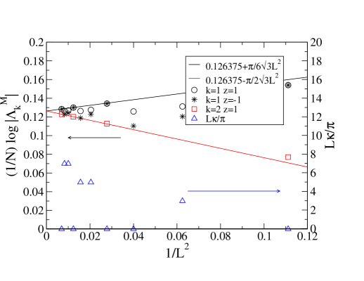
Figure 6: First eigenvalues of $T(1)$ and $T(-1)$ and the angle $\kappa$ defined by $\Lambda_{1}^{-}=|\Lambda_{1}^{-}|e^{\pm\imath\kappa}$. The lines are finite-size corrections to Baxter’s thermodynamic limit, $s_{\infty}=0.126375$, predicted from conformal invariance.

V.2.2 $L=3n\pm 1$ ($L$ not a multiple of three)

The first eigenvalue $\Lambda_{1}$ belongs to a triplet sector with conserved charges $(\frac{L}{3},\frac{L}{3},\frac{L}{3})\pm(\frac{2}{3},-\frac{1}{3},-\frac{1}{3})$, so that $\Lambda_{1}$ is three times degenerate. $\Lambda_{1}^{-}$ belongs to the $[3]$ or $[\bar{3}]$ triplet representation of SU(3) (except for $L=5$). It is found to be different from $\Lambda_{1}$ with $|\Lambda_{1}^{-}|<\Lambda_{1}$ (compare the stars with open circles in Fig. 6), so that at first order

$$Z_{3}\sim 3\Lambda_{1}^{M};\hskip 28.45274ptZ_{3}^{-}\sim\frac{3}{2}\Lambda_{1}^{M},$$ (23)

and $Z_{3}^{-}/Z_{3}$ goes to 1/2 when $M\rightarrow+\infty$ for infinitely long strips (as shown in Fig. 5). In this case not only the entropies are identical but also there is the same number of even and odd states: a $Z_{2}$ symmetry occurs.

Whereas $\Lambda_{1}$ must remain real (since $P(1)$ is a positive integer), $\Lambda_{1}^{-}=|\Lambda_{1}^{-}|e^{\imath\kappa}$ is complex in general (except for $L=5$). In this case, the complex-conjugate eigenvalue also occurs because $P(-1)$ is an integer (positive or negative). Thus the leading correction to the fraction of odd states reads

$$\frac{Z_{3}^{-}}{Z_{3}}\sim\frac{1}{2}-\alpha\left(\frac{|\Lambda_{1}^{-}|}{\Lambda_{1}}\right)^{M}\cos(\kappa M)+\dots$$ (24)

where $\alpha$ is the ratio of degeneracies and $|\Lambda_{1}^{-}|<\Lambda_{1}$. The convergence has oscillations in addition to the exponential decrease (see Fig. 5). It is peculiar that there are special aspect ratios where $Z_{3}^{-}/Z_{3}$ is very close to $1/2$ even for small $M$. This is the case of $L=4$ for $r=4/14(0.4999824)$, $4/18(0.49999948)$, $4/22(0.499999984)$ etc. (the larger the denominator, the closer to 1/2) and $L=10$ with $10/25(0.49938)$, $10/35(0.499969)$, $10/45(0.4999984)$, etc. These aspect ratios are of the form $2/p$ where $p$ is an odd integer. They correspond in fact to a cancelation of the oscillating part of Eq. 24, $\kappa M=\pi/2$ mod $\pi$. The convergence is then controlled by the next ratio of eigenvalues and is much faster.

It is a question as to whether in the thermodynamic limit aspect ratios other than zero may have a perfect Z₂ symmetry. Partly to address this question, we need to have access to larger system sizes and we will use a Monte-Carlo method with a modified algorithm.

VI Ergodic Monte-Carlo algorithm

We introduce a Monte-Carlo algorithm that does not conserve the parity of the chirality, by including the flip of “stranded” loops (examples are given in Fig. 7). We explicitly ckeck that this algorithm can reach all states on the clusters considered.

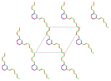
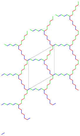
Figure 7: Triple-stranded loops make the algorithm ergodic by allowing parity changes. Black lozenges are the unit-cell, the loops are repeated outside the unit-cell for clarity (top, $N=108$, bottom $N=81$).

VI.1 Algorithm

In dimer models, loop Monte-Carlo algorithms that include all winding and nonwinding loops are ergodic. Indeed, given two dimer coverings, we can construct the “transition graph”, which consists of superimposing the two dimer coverings. The transition graph gives an ensemble of closed loops and individual dimers for edges both occupied by a dimer. Flipping all of its loops takes one state to the other, so that the states are connected by the motion of the loops.

In the three color model, the “transition graph” argument does not work. While it is possible to do the same operation for egdes in the, say, A state, this leaves the right loop configuration for the B-C sites (as explained in section III.1), with some sites already occupied and some empty, those that were previously A. The problem is that the empty sites cannot always be assigned a B or a C, since they are sometimes surrounded by exactly one B and one C: any assignement would violate the constraint. A way to solve the problem is to reorganize segments of the B-C loops, this is possible but it does not correspond to a loop motion.

In order to give a more clear picture of this, we have looked at the maximal overlap of two states belonging to two different sectors (this would give a single loop in the dimer problem). Two representative examples are given in Fig. 7: there we show only the edges that differ in color between the two states. In both cases, the loop is “stranded”: it forks at a given vertex into two segments that recombine at another vertex, either forming a short closed loop (an hexagon in the top figure) or a winding loop (bottom figure). An algorithm that would include these special moves will thus be able to bring the system from one sector to another.

A way to implement numerically these collective flips is through the introduction and annihilation of defects, i.e. local violations of the constraint. Recall first that flipping a two-color loop is equivalent to introducing two defects and annihilate them. First exchange the colors A-B of two neighboring edges. This creates a pair of defects with two neighbors in the same color, say A-A and B-B. Propagating them away from each other on the A-B loop by successively swapping A-B pairs, and recombining them at the end, exchanges the two colors of the whole loop. There are six such defectsMoore $q_{i}$ and $\bar{q}_{i}$, $i=A,B,C$: they are vertices with, among the three edges, one edge in color $i$ and two in the same color, thus violating the local constraint. Since two colors are available, they are denoted by $q$ or $\bar{q}$. With this notation, an A-B swap creates a pair of conjugate defects, which can propagate on the A-B loop and recombine,

$$\emptyset\rightarrow q_{C}+\bar{q}_{C}$$ (25)

$$q_{C}+\bar{q}_{C}\rightarrow\emptyset$$ (26)

This process is the standard flip of an entire A-B loop.

The other process that we exploit here is to create a triplet of defects $q_{A}$, $q_{B}$ and $q_{C}$ (or $\bar{q}_{A}$, $\bar{q}_{B}$ and $\bar{q_{C}}$) by exchanging the three colors at a given vertex, by a clockwise or anti-clockwise rotation (Fig. 8(a)). We propagate them away from the vertex on their respective two color loops until two of them meet (Fig. 8(b)). When they meet, they transform onto the conjugate defect of the third defect (Fig. 8(c)). It is then sufficient to further propagate the third defect until it annihilates with its conjugate (Fig. 8(d)). Once the first vertex and the orientation of the color exchange are chosen, the entire process is completely determined. The process $I_{i}^{+}$, where $i$ refers to a chosen vertex and $+$ to the orientation, is summarized as follows,

$$\emptyset\rightarrow q_{A}+q_{B}+q_{C}$$ (27)

$$q_{B}+q_{C}\rightarrow\bar{q}_{A}$$ (28)

$$q_{A}+\bar{q}_{A}\rightarrow\emptyset$$ (29)

and the conjugate process, $I_{i}^{-}$, consists of exchanging the three colors by the opposite rotation, $\emptyset\rightarrow\bar{q}_{A}+\bar{q}_{B}+\bar{q}_{C}$. Note that the process (28) may occur with any pair. The “time-reversal” process is not identical in general, in particular $I_{i}^{-}$ is not the reverse process: $I_{i}^{-}I_{i}^{+}\neq Id$. This is because in the last step [Eq. 29], the propagation of the $q_{A}$ defect may cross the first two segments. In this case, this leads to a local reorganisation of these segments. The process $I_{i}^{-}$ starts from the same vertex but does not find the same segments, since they have been reorganized. A new state different from the original state is generated. Such absence of microreversibility breaks the detailed balance and the Monte-Carlo algorithm would fail. We have therefore restricted explicitly the motion to those flips which satisfy $I_{i}^{+}I_{i}^{-}=Id$ (typically 40-50% depending on the size considered).

The Monte-Carlo algorithm works as follows: at each step we choose randomly whether to flip a loop or a “stranded” loop. If it is a “stranded” loop, we choose randomly a vertex and an orientation and create the triplet of defects that we propagate until they annihilate according to the description given above. We accept only the moves that are reversible.

We have checked on small lattices that we can now reach all states by successive application of these moves: for this we let the Monte-Carlo algorithm run until all distinct states are generated, the number of which we know from section III.1. We note that restricting it to short processes given in Fig. 7 (top), i.e. with two strands making a small hexagon, does change the parity but does not generate all states, so we have to include both. We therefore expect the present algorithm to be ergodic.

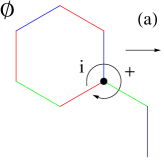
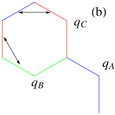
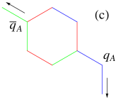
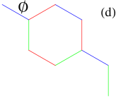
Figure 8: A way to implement numerically the flip of triple-stranded loops, by using defects: (a) from a perfect three-coloring ($\emptyset$), the three colors of the vertex $i$ marked by a point are exchanged, here clockwise $+$. (b) This generates three defects $q_{A}$ (BBR), $q_{B}$ (GGB) $q_{C}$ (RRG). $q_{B}$ propagates on a G-R loop, $q_{C}$ on a R-B loop (double arrows in (b)) until they annihilate $q_{B}+q_{C}\rightarrow\bar{q}_{A}$ (c). The last two defects propagate on a G-B loop and recombine in a perfect three-coloring $q_{A}+\bar{q}_{A}\rightarrow\emptyset$, resulting in the overall flip of a triple-stranded loop (d).

VI.2 Results

We have prepared samples of states by using the algorithm described above. In this dynamics, the parity is no longer conserved and the parity-parity autocorrelation function decays in less than a Monte-Carlo sweep ($N$ Monte-Carlo attempts).

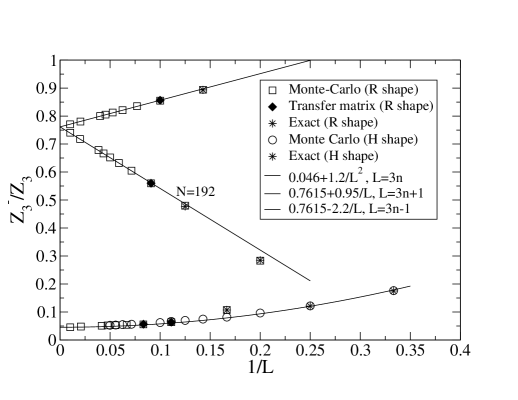
Figure 9: Fraction of odd states as a function of $1/L$ at fixed aspect ratio $r=1$, depending on mod($L,3$), obtained by Monte-Carlo algorithm (section VI.1), exact enumeration up to $L=8$ (section III.1) and transfer matrix up to $L=12$ (section V).

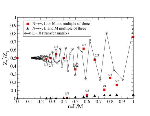
Figure 10: Fraction of odd states extrapolated in the thermodynamic limit (squares and triangles), as a function of the aspect ratio $r=L/M$, from Monte-Carlo. It depends on whether $L$ or $M$ are multiple of three. The results from transfer matrix at fixed $L=10$ (circles) are shown for comparison.

The first measurement is the fraction of odd states, $Z_{3}^{-}/Z_{3}$ in the sample of states. The result for $L=M$ is given in Fig. 9. For small clusters, we recover the exact results obtained by enumeration (table 3) and transfer matrix calculation (table 2). In the thermodynamic limit, we clearly see that the results extrapolate to a finite density, thus confirming that even and odd classes have the same entropy. For $L$ a multiple of three and for the rhombus shape or for all clusters with the hexagonal shape, the fraction is small, $0.046$ in the thermodynamic limit (bottom points in Fig. 9). Both are special in that they can accomodate the $\sqrt{3}\times\sqrt{3}$ state without domain walls. When $L=3n\pm 1$ is not a multiple of three, there are two distinct results (upper points in Fig. 9), which both converge linearly to a large fraction of odd states, $0.7615$. A majority of states is, therefore, missed by standard loop Monte-Carlo algorithms in this case.

We have done the same calculation for different aspect ratios $r=L/M$ and the results of similar extrapolations are summarized in Fig. 10. When $L$ and $M$ are multiples of three, the fraction remains small and smoothly interpolates between 0.046 for $r=1$ and 0 for $r=0$ (triangles in Fig. 10). When $L$ or $M$ is not a multiple of three, the fraction varies rapidly as a function of the aspect ratio (squares in Fig. 10). For comparison, we also give the result of the transfer matrix at finite $L=10$, where we have a fast-oscillating part. There may be, therefore, finite aspect ratios where the Z₂ symmetry found at $r=0$ holds as well. For instance, for $r=2/5$ or $2/7$, we cannot numerically distinguish the result from $Z_{3}^{-}/Z_{3}=1/2$.

The second measurement is the order-parameter of the $\sqrt{3}\times\sqrt{3}$ state, which was defined in section IV.2.1. $L$ has to be a multiple of three in this case and we know that the fraction of odd states is small, so we expect that the nonergodic algorithm has a small error. Nevertheless, the issue may be relevant since it was predicted that the Heisenberg model can be mapped onto the three-coloring problem with a finite interaction strength of a few percents, favoring long-range order of the $\sqrt{3}\times\sqrt{3}$ state.Chern The order-parameter we find from the ergodic algorithm follows the same power-law with $<m^{2}>\sim L^{-\eta}$ ($\eta=4/3$) as before, but with a shift in the logarithmic correction (Fig. 11). The result is in fact smaller by 4.4% (independent of $L$ at the numerical precision), reflecting that the small class of odd states has a much lower order-parameter. Moreover, since the estimate is lower, one needs a larger interaction to fit the Monte-Carlo data of the Heisenberg model,Chern that therefore strengthens the order predicted there.

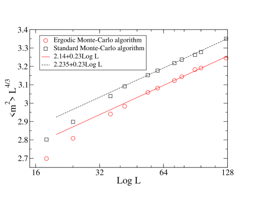
Figure 11: Order-parameter scaling of the $\sqrt{3}\times\sqrt{3}$ order, for both the standard loop Monte-Carlo algorithm (squares) and the present ergodic algorithm (circles) with periodic boundary conditions and $L=M=3n$. The systematic error when using the standard algorithm is 4.4%, which reflects the fraction of odd states given in Fig. 9.

VII Conclusion

We have shown that the total chirality of a three-coloring can be an odd or an even number and defines two classes. This parity is conserved by the loop dynamics because the lengths of the loops are even, when periodic boundary conditions are enforced. Previously-used loop Monte-Carlo algorithms are trapped in one sector and this explains the nonergodicity previously noted. This is true for the torus and Klein bottle, but not for the cylinder or plane where the loops can be of odd lengths.

The odd and even classes generically have the same entropy in the thermodynamic limit. An exception is the infinitely-long strip of hexagonal lattice with finite circumference $L$ where the entropy per site of the odd states is smaller than that of the even states by a universal correction, $8\pi/(\sqrt{3}L^{2})$, when $L$ is large and a multiple of three (Eq. 22). When $L$ is not a multiple of three, however, not only the entropies are identical, but also the number of odd and even states in the thermodynamic limit, so that the system has an infinite-temperature Z₂ symmetry. For general aspect ratio other than zero, this Z₂ symmetry is absent, but we assume it may exist at special points.

We have argued that “stranded” loops make the Monte-Carlo algorithm ergodic and allow to compute the fraction of odd states and order-parameters. By constrast, the standard loop algorithms that conserve parity lead to a systematic error, that can be large when $L$ is not a multiple of three. When $L$ is a multiple of three, however, the error on the order-parameter is of a few %, because, in this case, the odd class (although still extensive) is small.

Appendix A Enumeration of dimer coverings on hexagonal lattices

The method of enumeration of dimer coverings is known,Kasteleyn ; Fisher but the actual numbers for finite-size hexagonal lattices are known only in a few cases.Elser ; Schwandt We recall the method for completeness and for the discussion of appendix B and C.

A.1 Hexagonal shape with open boundary conditions

We consider the dimer problem on the hexagonal lattice shown in Fig. 2 with open boundary conditions. In this case, we recall thatKasteleyn ; Fisher

$$Z=\sum_{D}1=|\mbox{Pf}K|$$ (30)

where Pf is the Pfaffian of the Kasteleyn matrix $K$, defined by $K_{ij}=\pm 1$ if $i$ and $j$ are neighbours with the sign definition given in Fig. 2, $K_{ji}=-K_{ij}$. By definition, the Pfaffian of an antisymmetric matrix $K$ of even size $N$ is

$$\mbox{Pf}K=\sum_{P}\sigma(P)K_{i_{1}i_{2}}K_{i_{3}i_{4}}\cdots K_{i_{N-1},i_{N}}$$ (31)

with the restriction that $i_{1}<i_{2}$, $i_{3}<i_{4}$ etc. and $i_{1}<i_{3}<i_{5}\dots$. The sites $i_{1},i_{2},\dots$ are obtained by a permutation $P$ of $1,2,...,N$ and $\sigma(P)$ is its signature ($\sigma(P)=(-1)^{\#transpositions}=(-1)^{n_{e}}$ where $n_{e}$ is the number of even cycles). By an appropriate choice of signs of the matrix elements $K_{ij}$ one can compensate the negative sign of the permutation and obtain a sum over all configurations with weight 1, i.e. enumerate all states.Kasteleyn ; Fisher There are $N/2$ terms in the product of matrix elements. Kasteleyn showed that for the honeycomb lattice one has to choose a $-$ sign for the product of all signed edges around each hexagon, which is obtained by the choice given in Fig. 2. For a bipartite lattice, the matrix $K$ has the form,

$$K=\begin{pmatrix}0&D\\ -D^{T}&0\end{pmatrix}$$ (32)

and $\mbox{Pf}K=\pm\mbox{det}D$. It is therefore sufficient to compute a single determinant of a matrix of size $N/2\times N/2$. One can see it directly from the definition of the determinant, $\mbox{det}D=\sum_{P}\sigma(P)D_{1i_{1}}D_{2i_{2}}\cdots D_{N/2,i_{N/2}}$. The first indices $1,\dots,N/2$ denote the “black” sites and the second indices any permutation $P$ of the “white” sites. In this way every “black” site is paired to a “white” site, but we do not want long distance pairing so the matrix elements have to be zero except for the nearest neighbours. In this case, every site that is paired appears only once, and so every term in the sum corresponds to a dimer configuration. It is then important to fix the sign of the summand, so that each configuration is counted with the plus sign. Let us start with the reference configuration shown in Fig. 2, sometimes called the “empty room” by analogy with the problem of plane partitions.Elser In this configuration, the dimers are alternating in onion rings around the center. In terms of permutation, it is the identity, which consists of pairing a black site $i$ with the white site $i$. The product of $D_{ii}$ is positive, so that the reference configuration is counted with a plus sign (an alternative sign configuration is to take all arrows from black to white sites, in this case $K_{i,j}=+1$). Any cyclic motion around an hexagon corresponds to a cycle of odd length (half the length of the loop) that has a positive signature $(-1)^{l/2-1}=+1$, and a positive product of edges. Since any state can be reached through a sequence of cyclic motion, every dimer state is counted with a positive sign, and therefore

$$Z=\mbox{det}D.$$ (33)

The determinant of the $N/2\times N/2$ matrix $D$ is computed numerically and the results are given in table I. In fact, these numbers are known: the problem is exactly that of plane partitionsElser and the numbers of them for a $a\times b\times c$ hexagonal shape are the MacMahon numbers:

$$Z=\prod_{i=1}^{a}\prod_{j=1}^{b}\prod_{k=1}^{c}\frac{i+j+k-1}{i+j+k-2}$$ (34)

matching those in table 4 with $a=b=c=L$.

L	$Z$
1	2
2	20
3	980
4	232848
5	267227532
6	1478619421136
7	39405996318420160
8	5055160684040254910720
9	3120344782196754906063540800
10	9265037718181937012241727284450000
11	132307448895406086706107959899799334375000

Table 4: Numbers of dimer coverings with open boundary conditions, computed from the determinant or from the MacMahon formula (Eq. 34) with $a=b=c=L$.

A.2 Hexagonal shape with toroidal periodic boundary conditions

It is not possible to write the partition function as a single Pfaffian with periodic boundary conditions (the graph is not planar) since not all states can be reached with cyclic motion of hexagons. We need a linear combination of four Pfaffians.Kasteleyn The reference dimer state (Fig. 2) corresponds to the identity in terms of permutations and has a signature $+1$ and a positive product of oriented edges, for all weights $(u_{1},u_{2},u_{3})$ on the boundaries (for $x,y,z$ orientations). It has $L$ dimers along a line that cuts $3L$ edges (one is shown by a dashed line in Fig. 2) and there are three such lines along the three principal direction. Depending on the parity of $L$, the reference state has, therefore, either an (odd,odd,odd) or (even,even,even) number of dimers along the three directions: for odd $L$, all the states in the (odd,odd,odd) sector are counted with a plus sign. Now there are states that differ by a loop winding accross the boundaries, such a loop can change the parity of two sectors (so that the sum remains of the same parity as that of $L$), say 1 and 2, so the state is in a (odd,odd,even) sector for a reference state in a (even,even,even) sector. Since the winding loop also corresponds to an odd cycle, the signature of the new state does not change.

For this reason, the number of dimer coverings is

$$Z=\frac{1}{2}[\mbox{det}D(1,1,1)-\mbox{det}D(1,-1,-1)+$$

$$-(-1)^{L}\mbox{det}D(-1,-1,1)-(-1)^{L}\mbox{det}D(-1,1,-1)]$$ (35)

where $D(u_{1},u_{2},u_{3})$ is a Kasteleyn matrix with signs ($u_{1}=\pm 1,u_{2}=\pm 1,u_{3}=\pm 1$ and the constraint $u_{1}u_{2}u_{3}=1$) on the periodic boundaries, according to the three edge directions. The determinant of each $N/2\times N/2$ matrix $D$ is computed numerically and the results are given in Table 5. These numbers match those obtained by construction, in Table 1.

L	$Z$
1	6
2	120
3	15162
4	13219200
5	80478777786
6	3417194853335640
7	1010200119482131248768
8	2077088937091136948273774592
9	29688796156479320775456569461994826
10	2949240953029338499089605475162868134375000

Table 5: Numbers of dimer coverings $Z$ for the hexagonal shape with periodic boundary conditions, computed with four determinants (as in table 1 for $L\leq 4$). Some of these numbers were known.Schwandt

A.3 Rhombus shape with toroidal periodic boundary conditions

Here the shape of the cluster is that of a rhombus (Fig. 1). Without periodic boundary conditions, there is a single configuration, consisting of putting all dimers in the same direction, compatible with the boundaries (this is the identity in terms of permutation 1-1, 2-2 etc.). With periodic boundary conditions again the graph is nonplanar (with the exception of the $L=2$ cluster) and four Pfaffians are needed. The result is

$$Z=\frac{1}{2}|(-1)^{L+1}\mbox{det}D(1,1)+\mbox{det}D(-1,1)+$$

$$+\mbox{det}D(1,-1)+(-1)^{L}\mbox{det}D(-1,-1)|$$ (36)

where $D(u_{1},u_{2})$ is a Kasteleyn matrix with additional signs $(u_{1}=\pm 1,u_{2}=\pm 1)$ accross the two $(x,y)$ boundaries. The number of dimer configurations is given in table 6, in agreement with table 1.

L	$Z$
2	9
3	42
4	417
5	7623
6	263640
7	17886144
8	2249215617
9	547003370634
10	255635055079809
11	223497249280847919
12	379028233842678000000
13	1225114320423161720823183
14	7452791939816339215874217984
15	87934912263192096558472630935552
16	1969541555284024563005131046158940673

Table 6: Numbers of dimer coverings $Z$ for the rhombus shape with periodic boundary conditions (as in table 1 for $L\leq 8$).

Appendix B A general invariant in the dynamics of dimer coverings?

Each dimer covering has a possible invariant under dimer exchange along the loops,

$$I_{d}=\mbox{det}[n_{ij}D_{ij}(u_{1},u_{2})],$$ (37)

where $n_{ij}=1$ if there is a dimer on bond $ij$ and 0 otherwise, and $D_{ij}$ is the Kasteleyn matrix with $u_{1}$ and $u_{2}$ weights on the boundaries (on nonbipartite lattices, one has to replace the determinant by a Pfaffian, see appendix A). We first discuss the case $u_{1}=u_{2}=1$. On a planar graph, $I_{d}=1$ for all dimer coverings.Kasteleyn On a nonplanar graph, $I_{d}=\pm 1$ is in general not an invariant but it may remain invariant in a class of states. For instance in the problem of section A.3, $I_{d}=1$ for all states in the (even,even) class. This is ensured by the $\pi$ flux condition on each plaquette: a dimer permutation of a hexagon is a cycle of odd length so it has $\sigma(P)=1$ and a product of $D_{ij}>0$. Since all closed loops have length $4n+2$ on the honeycomb lattice, all cycles are odd and the invariant is therefore conserved. This is no longer true on a general lattice, as shown on the cubic lattice, where the flip of a square plaquette conserves $I_{d}$ (square cycles $(12)\rightarrow(21)$ have an odd signature, and the product of signed edges is odd, so that $I_{d}=1$).Freedman But there are longer closed loops that correspond to odd cycles and odd number of negative edges, so that in this case the invariant is restricted to moving the smallest loops.Freedman

On the honeycomb lattice with periodic boundary conditions of the torus geometry, this remains true for all closed loops and $I_{d}$ differs only in different winding sectors. For instance, in the rhombus case, $I_{d}=-1$ whenever the state belongs to a sector with $N^{x}$ or $N^{y}$ odd, or both odd. For a general $u_{1},u_{2}$, the considerations explained in appendix A lead to

$$I_{d}(u_{1},u_{2})=(-1)^{N^{x}+N^{y}+N^{x}N^{y}}u_{1}^{N^{x}}u_{2}^{N^{y}}.$$ (38)

Appendix C Alternative descriptions of the parity invariant

C.1 Product of signatures of permutations

We have seen that a three-coloring of the edges can be seen as three non-overlapping dimer coverings. Each dimer covering can be written as a permutation of the lattice sites, characterized by an invariant $I_{d}=\pm 1$ (see appendix B). We may thus define the quantity

$$I_{3}\equiv I_{d}(A)I_{d}(B)I_{d}(C)=\pm 1,$$ (39)

where $I_{d}(i)$ corresponds to the invariant $I_{d}$ of each of the three dimer coverings of color $i$. We show that $I_{3}$ is actually conserved by the motion of winding loops: when we flip an A-B winding loop, it corresponds to a cycle $C$ in the permutation of dimers $A$ and the cycle $C^{-1}$ in the permutation of dimers $B$. The product of these two cycles corresponds to exchanging $I_{d}(A)$ and $I_{d}(B)$, so that $I_{3}$ is constant. It turns out that $I_{3}$ equals to -1 in the odd sector and to +1 in the even sector (hence the same notation). Specifying to the rhombus shape with torus geometry, we have (see Eq. 38)

$$I_{d}(i)=(-1)^{N^{x}_{i}+N^{y}_{i}+N^{x}_{i}N^{y}_{i}}u_{1}^{N^{x}_{i}}u_{2}^{N^{y}_{i}}.$$ (40)

Noticing that $\sum_{i=1}^{3}N^{\alpha}_{i}=n$ is a constant that depends only on $L$, which we discard, we obtain

$$I_{3}=(-1)^{\sum_{i=1}^{3}N_{i}^{x}N_{i}^{y}}$$ (41)

Note that what is true for a pair $x,y$ of lattice directions is also true for the other pairs by symmetry. So that $I_{3}$ can be symmetrized and simplified,

$$I_{3}=(-1)^{\sum_{i=1}^{3}N_{i}^{x}N_{i}^{y}+N_{i}^{y}N_{i}^{z}+N_{i}^{z}N_{i}^{x}}=(-1)^{\frac{1}{2}\sum_{i\alpha}(N_{i}^{\alpha})^{2}}.$$ (42)

The argument $\frac{1}{2}\sum_{i\alpha}(N_{i}^{\alpha})^{2}$ is an even or odd integer. In this form, it is transparent that $I_{3}$ is invariant by all nonwinding loops, but is it remarkable that it remains invariant under winding loops as well.

C.2 Other related colorings

Fisk has studied a series of colorings and invariants.Fisk He showed that a 4-coloring of the sites of the triangular lattice induces a 3-coloring of the edges, which in turn induces a “Heawood” coloring of the sites and a local coloring. On a regular triangular lattice with open boundary conditions, we have the result that if $Z$ is the number of 3-colorings, $4Z$ is the number of 4-colorings.Baxter This is no longer true on a triangular lattice with periodic boundary conditions: starting from a valid 4-coloring of the sites, it is always possible to find an edge coloring.Fisk For completeness, we recall that the mapping associates to two neighbors of the triangular lattice a color of that bond, according to $(12)$ or $(34)$ gives color $1$ for the edge, $(13)$ or $(24)$ gives 2, and $(14)$ or $(23)$ gives 3. But the converse is not true: there are more three-colorings of the edges than 4-colorings (divided by four) of the sites. Fisk also defines a ”Heawood coloring” which is what is called the chirality here, and a “local” coloring which is an anti-domain wall separating sites of identical chirality. The number of such “singular edges” can be odd or even and is actually directly related to the number of vertices with positive chiralities.Fisk So that the odd/even invariant is also that of the number of anti-domain walls. No other simple invariants are known.Fisk

C.3 Odd/even invariant of graphs

The parity of $m$ turns out to be also related to the odd-even invariant recently introduced for colorings and graphs.Eager Let us make the connection explicit: given an orientation of the lattice, Eager and Lawrence count the number of oriented bonds $i\rightarrow j$ (where $i$ and $j$ are edges in our case) with $\sigma_{j}>\sigma_{i}$. The parity of this number is the “odd-even invariant”.Eager To make the connection with the parity of $m$ explicit, take each vertex, call the edges 1-2-3 clockwise and orient the bonds from edge 1 to edge 2, from edge 2 to edge 3, and from edge 1 to edge 3. All configurations with + (resp. -) chirality have one or three edges satisfying the rule above, i.e. an odd number $p$ of edges (resp. zero or two, i.e. an even number $n$ of edges). The total number of bonds satisfying the rule is $n_{e}=pN_{+}+nN_{-}$ where $N_{\pm}$ are the numbers of vertices with $\pm 1/2$ chirality (note that there are three bonds for each vertex). When $N_{+}$ is even, $N_{-}$ is even (because $N_{+}+N_{-}=2N/3$ is even) so $n_{e}$ is even. When $N_{+}$ is odd, $pN_{+}$ is odd and $nN_{-}$ is even, so $n_{e}$ is odd. Therefore a state with $I_{3}=\pm 1$ invariant is an even/odd state in the language of Ref. Eager, .

Appendix D Dimer and three-colorings on the Klein bottle

We consider the dimer and three-coloring problems on an hexagonal lattice with a “Klein bottle” geometry of the boundaries. The model is defined on finite-size clusters of size $L,M$ and rhombus shape; see Fig. 12 for an example. While the right boundary is identical to that of the torus, the upper boundary is flipped as in a Möbius strip, as shown by the arrows.

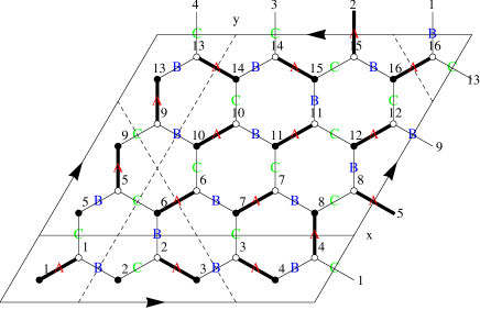
Figure 12: Hexagonal lattice with periodic boundary conditions of Klein bottle geometry, see the arrows on the sides. A dimer and color configurations are shown. Here a rhombus (R) shape is chosen with $L=4$ and $N=3L^{2}=48$ edges. The solid and dashed line show two distinct nonlocal cuts that define topological conserved numbers.

D.1 Exhaustive construction

We have constructed explicitly all the dimer coverings and three-colorings on the clusters with $L=M$ up to $L=8$. The numbers are given in table 7. On the Klein bottle, the three directions are nonequivalent and the number of dimer configurations is therefore no longer a multiple of three in general (but the number of three-colorings remains a multiple of six). The numbers are different from those obtained on the torus but remains of the same order of magnitude.

$N$	L	T	$Z^{K}$	$Z_{3}^{K}$
12	2	R	9	24
27	3	R	44	144
48	4	R	425	1,824
75	5	R	7,751	50,496
108	6	R	269,200	3,250,560
147	7	R	18,031,040	453,925,632
192	8	R	2,283,471,985	124,786,807,296

Table 7: Numbers of dimer coverings $Z^{K}$ and three-colorings $Z_{3}^{K}$ on the “Klein bottle” (rhombus shape, see Fig. 12). $Z^{K}$ is also calculated from Pfaffians and $Z_{3}^{K}$ from transfer matrix below.

D.2 Enumeration of dimers by Pfaffian

The number of dimer coverings on the Klein bottle has been studied in Refs. Lu, . It is given by

$$Z=|\mbox{Re}[\mbox{det}D((-1)^{L+1},\imath)]|+|\mbox{Im}[\mbox{det}D((-1)^{L},\imath)]|$$ (43)

where the matrix $D(u_{1},u_{2})$ is the Kasteleyn matrix deduced from Fig. 12 and $\imath^{2}=-1$ ensures the correct sign of the (even,even) sector. The determinant is computed numerically in table 8, and the numbers match those of table 7.

L	$Z^{K}$
2	9
3	44
4	425
5	7751
6	269200
7	18031040
8	2283471985
9	554296573020
10	257422540282721
11	226671176777404967
12	382906922419021541632
13	1233881647743136383304247
14	7553274215848727289369432064
15	88700806949845037589354602938368
16	1984263088240036324309600061358282721

Table 8: Numbers of dimer coverings $Z^{K}$ on the Klein bottle (rhombus shape), as in table 7 for $L\leq 8$.

D.3 Enumeration of three-colorings by transfer matrix

The enumeration of three-colorings by transfer matrix needs a simple modification with respect to the torus case. For the Klein bottle geometry, the first and the last row have to be images in a $x\rightarrow-x$ mirror symmetry, so we define an operator $P$ by $P|\sigma_{1}\dots\sigma_{L}\rangle=|\sigma_{L}\dots\sigma_{1}\rangle$ (with $P^{2}=1$). We then have

$$Z_{3}^{K}=\sum_{\sigma_{1}}\dots\sum_{\sigma_{M}}T_{\sigma_{1}\sigma_{2}}T_{\sigma_{2}\sigma_{3}}\cdots T_{\sigma_{M}\bar{\sigma_{1}}}=\mbox{Tr}[T^{M}P]$$ (44)

Because of the mirror symmetry, $[T,P]=0$, it is possible to simultaneously diagonalize $T$ and $P$, so that

$$Z_{3}^{K}=\mbox{Tr}[T^{M}P]=\sum_{i=1}^{3^{L}}\Lambda_{i}^{M}\pi_{i}$$ (45)

where $\pi_{i}=\pm 1$ is the parity of eigenvector $i$ under the mirror symmetry. We note that because of the Perron-Frobenius theorem for matrices with positive entries, the components of the largest eigenvector can be chosen to be positive. The eigenvector must be even, so that the sum $Z_{3}^{K}$ is positive, as it should be. Note that we cannot deduce that $Z_{3}^{K}<Z_{3}$ since the $\Lambda_{i}$ are complex. The result of the computation of the number of three-colorings on finite-size systems is given in table 10. A consequence of Eq. 45 is that $Z_{3}^{K}\sim\Lambda_{1}^{M}\sim Z_{3}$ in the thermodynamic limit $M\rightarrow+\infty$, so that the entropies of three-colorings on the Klein bottle or on the torus are the same.

D.4 Dynamics

We have studied the existence of sectors in the dynamics. For this, we have iterated the loop dynamics on finite-size clusters (up to $L=7$), starting from a single state and generating classes of states. Similarly to the torus case, there are winding-number sectors and Kempe sectors.

On the Klein bottle, there are also nontrivial cycles that define the winding sectors, but contrary to the torus, they are inequivalent. The cycle in the $x$ direction is identical to that of the torus, so that $N_{A}^{x}+N_{B}^{x}+N_{C}^{x}=L$ but the cycles in the $y$ or $z$ directions are twice longer and change direction at the boundary (see the dashed line in Fig. 12), $N_{A}^{y,z}+N_{B}^{y,z}+N_{C}^{y,z}=2M$.

We find one or two Kempe classes depending on $L$ in this case, up to lattice symmetries (table 9). We emphasize therefore that the number of Kempe classes depends explicitly on the geometry of the boundaries, since clusters with exactly the same number of sites do not have the same number of Kempe classes (compare tables 9 and 3).

Although the surface is nonorientable, we can define the chirality for vertices up to the upper cut. The parity of $m$ is again conserved and is given in table 9. The loop Monte-Carlo is therefore similarly nonergodic on the Klein bottle, and we use the “stranded” version to determine the fraction of odd states.

$N$	$n_{K}$	$Z^{K}_{i=1,\cdots,n_{K}}(\pm)$
12	1	24(+)
27	2	132(-),6(x2)(-)
48	2	1,056(+), 768(-)
75	2	36,096(-); 7,200(x2)(+)
108	2	2,600,448(+); 650,112(-)
147	2	249,212,928(-); 204,712,704(+)

Table 9: Number of invariant classes $n_{K}$ for clusters of size $N$ on the Klein bottle, and number of states in each class $Z^{K}_{i=1,\cdots,n_{K}}$ ($\sum_{i=1}^{n_{K}}n_{i}Z^{K}_{i}=Z^{K}_{3}$ is given in table 7)

D.5 Fraction of odd states from Monte-Carlo

We have computed the fraction of odd states by adding the “stranded” loops to the Monte-Carlo algorithm. We find that the result extrapolated to the thermodynamic limit is finite, confirming that odd and even classes also have the same entropy on the Klein bottle. The fraction now depends on mod$(L,6)$, but is partially resolved in the thermodynamic limit (Fig. 13), with pairs $6n\pm 1$, $6n\pm 2$ converging to the same value at the numerical precision, 0.55 and 0.445 respectively. If we write $p(L)=Z_{3}^{-}/Z_{3}$, we note (without providing an explanation) that $p(2L)+p(L)\approx 1$, which is specific to the Klein bottle.

In conclusion, the Klein bottle shares some aspects of the torus with the same parity invariant. For a Monte-Carlo algorithm to be ergodic, one has to similarly enrich the allowed motions with “stranded” loops. The odd and even classes have also the same entropy, as is obvious from Fig. 13.

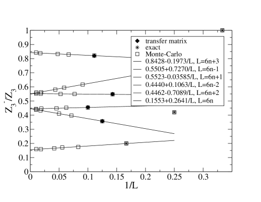
Figure 13: Fraction of odd states for finite-size clusters of size $L=M$, with the “Klein bottle” geometry. There is a mod($L,6$) effect, partially resolved in the thermodynamic limit.

$L$	$M$	$Z_{3}^{K}$	$Z_{3}^{K-}$
2	2	24	0
3	2	48	12
3	3	144	144
4	2	120	24
4	3	480	144
4	4	1824	768
5	2	288	132
5	3	1536	1248
5	4	8256	5712
5	5	50496	36096
6	2	744	240
6	3	5184	1296
6	4	39648	12576
6	5	350592	80640
6	6	3250560	650112
7	2	1872	1020
7	3	17952	13488
7	4	194304	116976
7	5	2471424	1523904
7	6	32740992	18050880
7	7	453925632	249212928
8	2	4824	1800
8	3	62688	15120
8	4	956832	310080
8	5	17236608	5086080
8	6	323501184	104595840
8	7	6307763712	2120299776
8	8	124786807296	44607627264
9	2	12288	7092
9	3	219168	164016
9	4	4704192	3012240
9	5	121491456	86064576
9	6	3291241344	2339395392
9	7	93849672192	71017214208
9	8	2743266960384	2153241150720
9	9	82222744421376	67451020701696
10	2	31560	12384
10	3	767136	189072
10	4	23256672	8270688
10	5	860378112	291036480
10	6	33588864384	13048871040
10	7	1385171841024	552878592000
10	8	58393359785472	24928794444288
10	9	2514348535314432	1105303915459584
10	10	109522261290792960	49879717261246464

Table 10: Numbers of 3-colorings on the “Klein bottle”, $Z_{3}^{K}$, computed by numerical transfer matrix, for system size $N=3\times L\times M$ (Fig. 12). $Z_{3}^{K-}$ is the number of odd colorings.

References

- (1) M. E. J. Newman and G. T. Barkema, Monte-Carlo Methods in Statistical Physics, Oxford University Press, 1999.
- (2) A. Rahman and F. H. Stillinger, J. Chem. Phys. 57, 4009 (1972).
- (3) J.-S. Wang, R. H. Swendsen, and R. Kotecky, Phys. Rev. Lett. 63, 109 (1989).
- (4) O. Sikora, N. Shannon, F. Pollmann, K. Penc, and P. Fulde, Phys. Rev. B 84, 115129 (2011).
- (5) M. Freedman, M. B. Hastings, C. Nayak, and X.-L. Qi, Phys. Rev. B 84, 245119 (2011).
- (6) R. J. Baxter, J. Math. Phys. 11, 784 (1970).
- (7) D. A. Huse and A. D. Rutenberg, Phys. Rev. B 45, 7536 (1992), see reference [13] therein.
- (8) B. Mohar and J. Salas, J. Stat. Mech. P05016 (2010).
- (9) C. Moore and M. E. J. Newman, J. Stat. Phys. 99, 629-660 (2000).
- (10) C. Castelnovo, C. Chamon, C. Mudry, and P. Pujol, Phys. Rev. B 72, 104405 (2005).
- (11) O. Cépas and A. Ralko, Phys. Rev. B 84, 020413 (2011).
- (12) L. B. Ioffe, M. Feigel’man, A. Ioselevich, D. Ivanov, M. Troyer, and G. Blatter, Nature 415, 503 (2002).
- (13) Periodic boundary conditions may be achieved by connecting opposite sides or from three-dimensional lithography.
- (14) A. Müller, M. Luban, C. Schroeder, R. Modler, P. Kögerler, M. Axenovich, J. Schnack, P. Canfield, S. Bud’ko, and N. Harrison, ChemPhysChem 2, 517 (2001).
- (15) P. Fendley, J. E. Moore and C. Xu, Phys. Rev. E 75, 051120 (2007).
- (16) S. E. Korshunov, F. Mila, and K. Penc, Phys. Rev. B 85, 174420 (2012).
- (17) We construct numerically all the dimer coverings by making a tree. Each node of the tree corresponds to a cluster partially-filled with dimers and the generation of a new node consists of adding a dimer on neighboring empty sites. Only the final leaves may be proper dimer coverings. The tree is being traversed by using a “depth-first search” method which adds nodes along a branch, before backtracking when a valid or an invalid configuration is obtained. It has the advantage to minimize the need of memory, by keeping a single branch of the tree, i.e. partial states. The states themselves can be kept in memory for small sizes or analysed on the fly.
- (18) This method allows to work with 128-bit integers and compute the exact number of configurations up to . Higher exact numbers need using multiprecision packages.
- (19) P. Chandra, P. Coleman, I. Ritchey, J. Phys. I France 3, 591 (1993).
- (20) B. Chakraborty, D. Das, and J. Kondev, Eur. Phys. J. E 9, 227 (2002).
- (21) C. Castelnovo, P. Pujol, and C. Chamon, Phys. Rev. B 69, 104529 (2004).
- (22) Gia-Wei Chern and R. Moessner, Phys. Rev. Lett. 110, 077201 (2013).
- (23) O. Cépas and B. Canals, Phys. Rev. B 86, 024434 (2012); O. Cépas, Phys. Rev. B 90, 064404 (2014).
- (24) To know whether a state is new or not (and avoid cycles), we construct a hash table where we insert the new states. We keep all states in memory to analyze the collisions in the hash table. A compact way to store the states is to use a single bit for the chirality of each vertex (see section IV.2.1 for the definition). The honeycomb lattice is bipartite and, as the largest size considered has sites ( edges) we need at most two 64-bit integers (which we hash). In constrast, a direct color coding would need two bits per edge, i.e. three times more memory. Note that once the color of a first site is fixed all other sites are uniquely determined by the chiralities: there are three times more color configurations than chirality configurations. By symmetry, we can also impose the chirality of the first site to be +, so that we need to keep only states in memory. For , this requires Go of memory, but Go for , which is beyond our capabilities.
- (25) S.-M. Belcastro and R. Haas, Discrete Mathematics, 325, 77 (2014).
- (26) For , we cannot keep all states in memory (see [technical, ]), so we proceed differently to construct the Kempe sectors. For each state in a given topological sector, we record all the topological sectors it is linked to by flipping a winding loop. In a second time, we construct closed orbits obtained by applying this link matrix iteratively: each sector becomes a class of topological sectors and we assume in this way that sectors that have the same topological numbers are always connected, which is true for all the smaller clusters. The result is therefore a lower bound for .
- (27) L. Jaubert, J. T. Chalker, P. C. W. Holdsworth, and R. Moessner, Phys. Rev. Lett. 105, 087201 (2010).
- (28) N. Read(unpublished).
- (29) J. Kondev and C. Henley, Nucl. Phys. 464, 540 (1996).
- (30) P. W. Kasteleyn, Physica 27, 1209 (1961).
- (31) M. E. Fisher, Phys. Rev. 124, 1664 (1961).
- (32) V. Elser, J. Phys. A: Math. Gen. 17, 1509 (1984).
- (33) D. Schwandt, Ph. D thesis, University of Toulouse (2011), https://tel.archives-ouvertes.fr/tel-00783224v1, p. 30; and G. Misguich (private communication).
- (34) S. Fisk, Adv. in Math. 25, 226 (1977).
- (35) R. Eager and J. Lawrence, Eur. J. of Combinatorics, 50, 87 (2015).
- (36) W. T. Lu and F. W. Wu, Phys. Lett. A 293, 235 (2002); W. Li and H. Zhang, Physica A 391, 3833 (2012).