A stabilized Nitsche cut finite element method for the Oseen problem

Abstract

We propose a stabilized Nitsche-based cut finite element formulation for the Oseen problem in which the boundary of the domain is allowed to cut through the elements of an easy-to-generate background mesh. Our formulation is based on the continuous interior penalty (CIP) method of Burman et al. [1] which penalizes jumps of velocity and pressure gradients over inter-element faces to counteract instabilities arising for high local Reynolds numbers and the use of equal order interpolation spaces for the velocity and pressure. Since the mesh does not fit the boundary, Dirichlet boundary conditions are imposed weakly by a stabilized Nitsche-type approach. The addition of CIP-like ghost-penalties in the boundary zone allows to prove that our method is inf-sup stable and to derive optimal order a priori  error estimates in an energy-type norm, irrespective of how the boundary cuts the underlying mesh. All applied stabilization techniques are developed with particular emphasis on low and high Reynolds numbers. Two- and three-dimensional numerical examples corroborate the theoretical findings. Finally, the proposed method is applied to solve the transient incompressible Navier-Stokes equations on a complex geometry.

url]www.andremassing.com

url]www.lnm.mw.tum.de/staff/benedikt-schott

url]www.lnm.mw.tum.de/staff/wall

1 Introduction

Many important phenomena in science and engineering are modeled by a system of partial differential equations (PDEs) posed on complicated, three-dimensional domains. The numerical solution of PDEs based on the finite element method requires the generation of high quality meshes to ensure both a proper geometric resolution of the domain features and good approximation properties of the numerical scheme. But even today, the generation of such meshes can be a time-consuming and challenging task that can easily account for large portions of the time and human resources in the overall simulation work flow. For instance, the simulation of many industrial application problems requires a series of highly non-trivial preprocessing steps to transform CAD data into conforming domain discretizations which respect complicated features of the geometric model. The problem is even more pronounced if the geometry of the model domain changes substantially in the course of the simulation, e.g., in the simulation of multiphase flows, where the interface between different fluid phases can undergo large and even topological changes when bubbles merge or break up or drops pinch off. Then even modern Arbitrary-Lagrangian-Eulerian based mesh moving algorithms break down and a costly remeshing is the only resort.

A potential remedy to these challenges are flexible, so-called unfitted finite element schemes which allow to embed complex or changing domain parts freely into a static and easy-to-generate computational domain. For instance, to cope with large interface motion in incompressible two-phase flows, the discretization schemes in [2, 3, 4, 5] combined an implicit, level set based description of the fluid phase interface with an extended finite element approach. For fluid-structure interaction problems where the structure might undergo large deformations, numerical methods which combine fixed-grid Eulerian approach for the fluid with a Lagrangian description for the structural body have been developed in, e.g., [6, 7, 8, 9], including three-dimensional fluid-structure-contact interactions [10]. Furthermore, in several numerical schemes aiming at complex fluid-structure interactions the idea of using finite element method on composite grids, originally proposed in [11], has been picked up. In [12, 13, 14], an additional fluid patch covering the boundary layer region around structural bodies is embedded into a fixed-grid background fluid mesh to possibly capture high velocity gradients near the structure when simulating high-Reynolds-number incompressible flows.

As the computational mesh is not fitted to the domain boundary, a common theme of the aforementioned unfitted finite element approaches is the weak imposition of boundary or interface conditions posed on parts of the embedded domain by means of Lagrange multipliers or Nitsche-type methods, see, e.g., [15, 8, 12, 16, 17]. Building upon and extending these ideas, the cut finite element method (CutFEM) as a particular unfitted finite element framework has gained rapidly increasing attention in science and engineering, see [18] for a recent overview. A distinctive feature of the CutFEM approach is that it provides a general, theoretically founded stabilization framework which, roughly speaking, transfers stability and approximation properties from a finite element scheme posed on a standard mesh to its cut finite element counterpart. As a result, a wide range of problem classes, ranging from two-phase and fluid-structure interaction problems [5, 13] to surface and surface-bulk PDEs [19, 20, BurmanHansboLarsonEtAl2016c, 21], and embedding methods such as overlapping meshes  [11, Massing2012, 22, 23, 14] or implicitly defined surfaces [19, 18], has been treated by CutFEM based discretization schemes in a transparent and unified way. However, for fluid related problems, stability and a priori error analysis of CutFEM type approaches has only been performed for simplified prototype problems, such as the Poisson problem [16, 17], the Stokes problem [24, 23, 4, 25], and recently, for a low Reynolds-number fluid-structure interaction problem governed by Stokes’ equations in [26]. For more complex fluid problems governed by the transient incompressible Navier-Stokes equations at high Reynolds numbers, there is a lack of numerical analysis.

In the present work we propose and analyze a cut finite element method for the Oseen model problem. The Oseen problem comprises a set of linear equations which naturally arise in many linearization and time-stepping methods for the transient, non-linear incompressible Navier-Stokes equations. Our formulation is based on the continuous interior penalty (CIP) method of Burman et al. [1] which penalizes jumps of velocity and pressure gradients over inter-element faces to counteract instabilities arising for high local Reynolds numbers and the use of equal order interpolation spaces for the velocity and pressure. Since the mesh does not fit the boundary, Dirichlet boundary conditions are imposed weakly by a stabilized Nitsche-type approach. In contrast to [1], additional measures are necessary to prove that the proposed scheme is inf-sup stable and satisfies optimal order a priori  error estimates irrespective of how the boundary cuts the underlying mesh. Extending the approach taken in [27, 17, 24, 23] to provide geometrically robust a priori  error and condition number estimates for the Poisson and Stokes problem, our method uses different face-based ghost-penalty stabilizations for the velocity and pressure fields which are defined in the vicinity of the embedded boundary. In [28], it was shown how these interface-zone stabilization techniques can be naturally combined with the continuous interior penalty method from [1] to solve transient convection-dominant incompressible Navier-Stokes equations on cut meshes. However, so far a numerical analysis of that method was still outstanding. The present paper now provides the theoretical corroboration of the fluid formulation introduced in [28] with focus on the different ghost-penalty stabilizations in the high-Reynolds-number regime.

A main challenge in the presented numerical analysis is to compensate the lack of a suitable CutFEM variant of the $L^{2}$ projection operator which in the fitted mesh case is an instrumental tool in the theoretical analysis of CIP stabilized methods. As a remedy, we derive stability and approximation results for norms which are more natural in residual-based stabilization methods for the Oseen problem. This approach allows to employ alternative interpolation operators such as the Clément operator for which proper CutFEM counterparts can be defined. By adding suitable ghost-penalty stabilizations we gain sufficient control over the advective derivative and the incompressibility constraint with respect to the entire active part of the computational mesh. Consequently, we are able to prove that our scheme obeys an inf-sup condition in a ghost-penalty enhanced energy-type norm and thus satisfies the corresponding a priori  energy norm error estimate. All estimates are optimal independent of the positioning of the boundary within the non-boundary fitted background mesh. For the first time, we present a numerical analysis for ghost-penalty operators scaled with non-constant coefficients accounting for different flow regimes, covering the treatment of instabilities arising from the convective term and from the incompressibility constraint on cut meshes. As a by-product of our numerical analysis, we show how the continuous interior penalty stabilization terms give control over slightly stronger norm contributions as they typically arise in residual-based stabilization method [29, 30].

The paper is organized as follows: We conclude this section by summarizing our basic notation. Then the Oseen model problem is briefly reviewed in Section 2. In Section 3, we formulate the stabilized Nitsche-type cut finite element method for the Oseen problem, starting with the introduction of the proper cut finite element spaces, followed by a review of the classical continuous interior penalty (CIP) method. We explain how to extend the CIP scheme to the case of unfitted meshes, discuss the need for additional ghost-penalty stabilization techniques in the vicinity of the boundary zone for low and high Reynolds numbers, and conclude this section by stating the main a priori  estimate for our cut finite element method. Next, two- and three-dimensional test cases in Section 4 confirm the main theoretical result. The applicability of our method to solve transient incompressible Navier-Stokes equations is demonstrated by means of a challenging complex three-dimensional helical pipe flow. Afterwards, we present the numerical analysis of our proposed formulation. In Section 5, basic approximation properties, interpolation operators and norms are introduced and the importance of the different ghost-penalty terms is elaborated. Sections 6 and 7 are devoted to the stability and a priori  error analysis of the proposed method. Therein, main focus is directed to inf-sup stability and optimality of the error estimates in all flow regimes. Summarizing comments and an outlook to potential application fields for our numerical scheme in Section 8 conclude this work.

1.1 Basic Notation

Throughout this work, $\Omega\subset\mathbb{R}^{d}$, $d=2,3$ denotes an open and bounded domain with Lipschitz boundary $\Gamma=\partial\Omega$. For $U\in\{\Omega,\Gamma\}$ and $0\leqslant m<\infty$, $1\leqslant q\leqslant\infty$, let $W^{m,q}(U)$ be the standard Sobolev spaces consisting of those $\mathbb{R}$-valued functions defined on $U$ which possess $L^{q}$-integrable weak derivatives up to order $m$. Their associated norms are denoted by $\|\cdot\|_{m,q,U}$. As usual, we write $H^{m}(U)=W^{m,2}$ and $(\cdot,\cdot)_{m,U}$ and $\|\cdot\|_{m,U}$ for the associated inner product and norm. If unmistakable, we occasionally write $(\cdot,\cdot)_{U}$ and $\|\cdot\|_{U}$ for the inner products and norms associated with $L^{2}(U)$, with $U$ being a measurable subset of $\mathbb{R}^{d}$. For $s>1/2$, we use the notation $[H_{\boldsymbol{g}}^{s}(\Omega)]^{d}$ to denote the set of all $\mathbb{R}^{d}$-valued functions in $[H^{s}(\Omega)]^{d}$ whose boundary traces are equal to $\boldsymbol{g}$. Moreover, $H_{0}(\nabla\cdot;\Omega)\subset[L^{2}(U)]^{d}$ denotes the space of divergence-free functions, and $L^{2}_{0}(\Omega)$ denotes the function space consisting of functions $u\in L^{2}(\Omega)$ with zero average. Finally, any norm $\|\cdot\|_{\mathcal{P}_{h}}$ used in this work which involves a collection of geometric entities $\mathcal{P}_{h}$ should be understood as broken norm defined by $\|\cdot\|_{\mathcal{P}_{h}}^{2}=\sum_{P\in\mathcal{P}_{h}}\|\cdot\|_{P}^{2}$ whenever $\|\cdot\|_{P}$ is well-defined, with a similar convention for scalar products $(\cdot,\cdot)_{\mathcal{P}_{h}}$.

2 The Oseen Problem

After applying a time discretization method and a linearization step, many solution algorithms for the non-linear Navier-Stokes equations can be reduced to solving a sequence of auxiliary problems of Oseen type for the velocity field $\boldsymbol{u}$ and the pressure field $p$:

$$\sigma\boldsymbol{u}+\boldsymbol{\beta}\cdot\nabla\boldsymbol{u}-\nabla\cdot(2\mu{\boldsymbol{\epsilon}}(\boldsymbol{u}))+\nabla p =\boldsymbol{f}\quad \text{ in }\Omega,$$ (2.1)

$$\nabla\cdot\boldsymbol{u} =0\quad \text{ in }\Omega,$$ (2.2)

$$\boldsymbol{u} =\boldsymbol{g}\quad \text{ on }\Gamma.$$ (2.3)

Here, ${\boldsymbol{\epsilon}}(\boldsymbol{u})=1/2(\nabla\boldsymbol{u}+(\nabla\boldsymbol{u})^{T})$ denotes the rate-of-deformation tensor, $\boldsymbol{\beta}\in[W^{1,\infty}(\Omega)]^{d}\cap H_{0}(\nabla\cdot;\Omega)$ the given divergence-free advective velocity field, $\boldsymbol{f}\in[L^{2}(\Omega)]^{d}$ the body force and $\boldsymbol{g}\in[H^{1/2}(\Gamma)]^{d}$ the given boundary data. The reaction coefficient $\sigma$ and the viscosity $\mu$ are assumed to be positive real-valued constants. The corresponding weak formulation of the Oseen problem (2.1)–(2.3) is to find the velocity and the pressure field $(\boldsymbol{u},p)\in\mathcal{V}_{\boldsymbol{g}}\times\mathcal{Q}=[H_{\boldsymbol{g}}^{1}(\Omega)]^{d}\times L^{2}_{0}(\Omega)$ such that

$$a(\boldsymbol{u},\boldsymbol{v})+b(p,\boldsymbol{v})-b(q,\boldsymbol{u})=l(\boldsymbol{v})\quad\forall\,(\boldsymbol{v},q)\in\mathcal{V}_{\boldsymbol{0}}\times\mathcal{Q},$$ (2.4)

where

$$a(\boldsymbol{u},\boldsymbol{v}) :=(\sigma\boldsymbol{u},\boldsymbol{v})_{\Omega}+(\boldsymbol{\beta}\cdot\nabla\boldsymbol{u},\boldsymbol{v})_{\Omega}+(2\mu{\boldsymbol{\epsilon}}(\boldsymbol{u}),{\boldsymbol{\epsilon}}(\boldsymbol{v}))_{\Omega},$$ (2.5)

$$b(p,\boldsymbol{v}) :=-(p,\nabla\cdot\boldsymbol{v})_{\Omega},$$ (2.6)

$$l(\boldsymbol{v}) :=(\boldsymbol{f},\boldsymbol{v})_{\Omega}.$$ (2.7)

The well-posedness and solvability of the continuous problem (2.4) is well-known, see for instance the textbook by Girault and Raviart [31].

3 A Cut Finite Element Method for the Oseen Problem

3.1 Computational Meshes and Cut Finite Element Spaces

Let $\widehat{\mathcal{T}}_{h}=\{T\}$ be a quasi-uniform mesh consisting of shape-regular simplices $T$ with mesh size parameter $h$ which covers the physical domain $\Omega$. For the background mesh $\widehat{\mathcal{T}}_{h}$ we define the active (background) mesh

$$\mathcal{T}_{h}:=\{T\in\widehat{\mathcal{T}}_{h}:T\cap\Omega\neq\emptyset\},$$ (3.1)

consisting of all elements in $\widehat{\mathcal{T}}_{h}$ which intersect $\Omega$. Denoting the union of all elements $T\in\mathcal{T}_{h}$ by $\Omega^{\ast}_{h}$, we call $\mathcal{T}_{h}$ a fitted mesh if $\overline{\Omega}=\overline{\Omega^{\ast}_{h}}$ and an unfitted mesh if $\overline{\Omega}\subsetneq\overline{\Omega^{\ast}_{h}}$. To each active mesh, we associate the subset of elements that intersect the boundary $\Gamma$

$$\mathcal{T}_{\Gamma}:=\{T\in\mathcal{T}_{h}:T\cap\Gamma\neq\emptyset\}.$$ (3.2)

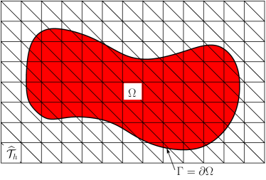
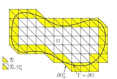
Figure 3.1: Left: The physical domain $\Omega$ is defined as the inside of a given boundary $\Gamma$ embedded into a fixed background mesh $\widehat{\mathcal{T}}_{h}$. Right: The fictitious domain $\Omega^{\ast}_{h}$ is the union of the minimal subset $\mathcal{T}_{h}\subset\widehat{\mathcal{T}}_{h}$ covering $\Omega$.

The set of all facets, i.e. edges of elements in two dimensions and faces of elements in three dimensions, are denoted by $\mathcal{F}_{h}$. We let $\mathcal{F}_{i}$ be the set of all interior facets $F$ which are shared by exactly two elements, denoted by $T^{+}_{F}$ and $T^{-}_{F}$. Further, we introduce the notation $\mathcal{F}_{\Gamma}$ for the set of all interior facets belonging to elements intersected by the boundary $\Gamma$,

$$\mathcal{F}_{\Gamma}:=\{F\in\mathcal{F}_{i}:\;T^{+}_{F}\cap\Gamma\neq\emptyset\vee T^{-}_{F}\cap\Gamma\neq\emptyset\}.$$ (3.3)

To ensure that $\Gamma$ is reasonably resolved by $\mathcal{T}_{h}$, we require that the quasi-uniform $\mathcal{T}_{h}$ and the boundary $\Gamma$ satisfy the following geometric conditions from [32, 17, 33, 25]:

• G1: The intersection between $\Gamma$ and a facet $F\in\mathcal{F}_{i}$ is simply connected; that is, $\Gamma$ does not cross an interior facet multiple times.

• G2: For each element $T$ intersected by $\Gamma$, there exists a plane $S_{T}$ and a piecewise smooth parametrization $\Phi:S_{T}\cap T\rightarrow\Gamma\cap T$.

• G3: We assume that there is an integer $N>0$ such that for each element $T\in\mathcal{T}_{\Gamma}$, there exists an element $T^{\prime}\in\mathcal{T}_{h}\setminus\mathcal{T}_{\Gamma}$ and at most $N$ elements $\{T\}_{j=1}^{N}$ such that $T_{1}=T,\,T_{N}=T^{\prime}$ and $T_{j}\cap T_{j+1}\in\mathcal{F}_{i},\;j=1,\ldots,N-1$. In other words, the number of facets to be crossed in order to “walk” from a cut element $T$ to a non-cut element $T^{\prime}\subset\Omega$ is bounded.

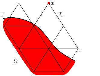
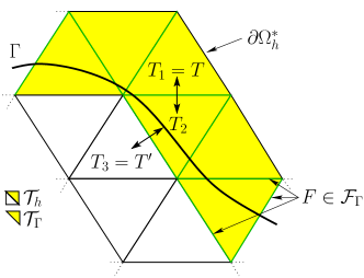
Figure 3.2: The boundary zone of the fictitious domain. Left: The background mesh $\mathcal{T}_{h}$ and the physical domain $\Omega$. Observe that for the elements associated with the node $\boldsymbol{x}$, only a small fraction resides inside the domain $\Omega$. Right: Elements colored in yellow are intersected by the boundary and are therefore part of the mesh $\mathcal{T}_{\Gamma}$. Interior facets belonging to elements intersected by the boundary ($\mathcal{F}_{\Gamma}$) are marked in green. Arrows indicate the shortest “walk” from cut element $T$ to an uncut element $T^{\prime}$.

Figures 3.1 and 3.2 summarize the notation. Next, for a given mesh $\mathcal{T}_{h}$, we denote by $\mathcal{X}_{h}$ the finite element spaces consisting of continuous piecewise polynomials of order $k$

$$\mathcal{X}_{h} =\left\{v_{h}\in C^{0}(\Omega^{\ast}_{h}):\left.v_{h}\right|_{T}\in\mathcal{P}^{k}(T)\,\forall\,T\in\mathcal{T}_{h}\right\}.$$ (3.4)

Using equal order interpolation spaces, the discrete velocity space $\mathcal{V}_{h}$, the discrete pressure space $\mathcal{Q}_{h}$ and the total approximation space $\mathcal{W}_{h}$ are then defined by

$$\mathcal{V}_{h}=[\mathcal{X}_{h}]^{d},\quad\mathcal{Q}_{h}=\mathcal{X}_{h},\quad\mathcal{W}_{h}=\mathcal{V}_{h}\times\mathcal{Q}_{h}.$$ (3.5)

3.2 A Short Review of the Continuous Interior Penalty Method for the Oseen Problem

Assuming for the moment that $\mathcal{T}_{h}$ is a fitted tessellation of $\Omega$, it is well-known that a direct discretization of the weak formulation (2.4) using equal-order interpolation spaces $\mathcal{W}_{h}=\mathcal{V}_{h}\times\mathcal{Q}_{h}$ suffers from two problems. First, the resulting scheme does not satisfy an inf-sup condition and consequently, is not stable in the sense of Babuška–Brezzi [34]. Second, it leads to spurious oscillations in the numerical solution and sub-optimal error estimates in the case of convection-dominant flow. To counteract both effects, the discrete form (2.4) typically needs to be stabilized, see [30] for an overview over various stabilization techniques for finite element based discretizations of the Oseen problem.

In this work, we employ the continuous interior penalty (CIP) method proposed by Burman et al. [1], which is a symmetric stabilization technique penalizing the jump of the velocity and pressure gradients over element facets. More precisely, the stabilization operators are defined by

$$s_{\beta}(\boldsymbol{u}_{h},\boldsymbol{v}_{h}) :=\gamma_{\beta}\sum_{F\in\mathcal{F}_{i}}\langle\phi_{\beta}\rangle|_{F}h(\llbracket\boldsymbol{\beta}\cdot\nabla\boldsymbol{u}_{h}\rrbracket,\llbracket\boldsymbol{\beta}\cdot\nabla\boldsymbol{v}_{h}\rrbracket)_{F},$$ (3.6)

$$s_{u}(\boldsymbol{u}_{h},\boldsymbol{v}_{h}) :=\gamma_{u}\sum_{F\in\mathcal{F}_{i}}\langle\phi_{u}\rangle|_{F}h(\llbracket\nabla\cdot\boldsymbol{u}_{h}\rrbracket,\llbracket\nabla\cdot\boldsymbol{v}_{h}\rrbracket)_{F},$$ (3.7)

$$s_{p}(p_{h},q_{h}) :=\gamma_{p}\sum_{F\in\mathcal{F}_{i}}\langle\phi_{p}\rangle|_{F}h(\llbracket\boldsymbol{n}_{F}\cdot\nabla p_{h}\rrbracket,\llbracket\boldsymbol{n}_{F}\cdot\nabla q_{h}\rrbracket)_{F},$$ (3.8)

where for any, possibly vector-valued, piecewise discontinuous function $\phi$ on $\mathcal{T}_{h}$, the jump $\llbracket\phi\rrbracket$ and average $\langle\phi\rangle$ over an interior facet $F\in\mathcal{F}_{i}$ is given by

$$\llbracket\phi\rrbracket|_{F}=(\phi_{F}^{+}-\phi_{F}^{-}),\qquad\langle\phi\rangle|_{F}=\tfrac{1}{2}(\phi_{F}^{+}+\phi_{F}^{-}),$$ (3.9)

with $\phi^{\pm}(\boldsymbol{x})=\lim_{t\to 0^{+}}\phi(\boldsymbol{x}\pm t\boldsymbol{n}_{F})$ for some chosen normal unit vector $\boldsymbol{n}_{F}$ on $F$. The element-wise constant stabilization parameters $\phi_{\beta}$, $\phi_{u}$ and $\phi_{p}$ are chosen as

$$\phi_{u,T}=\mu+\|\boldsymbol{\beta}\|_{0,\infty,T}h+\sigma h^{2},\qquad\phi_{\beta,T}=\phi_{p,T}=\dfrac{h^{2}}{\mu+\|\boldsymbol{\beta}\|_{0,\infty,T}h+\sigma h^{2}}.$$ (3.10)

To ease the notation we often simply write $\phi_{\beta,F}$, $\phi_{u,F}$, and $\phi_{p,F}$ for their respective face averages. Note that since $\boldsymbol{\beta}\in[W^{1,\infty}(\Omega)]^{d}\subseteq[C^{0,1}(\Omega)]^{d}$ it holds that $\boldsymbol{\beta}$ is (Lipschitz)-continuous by assumption and therefore $\boldsymbol{\beta}\cdot\boldsymbol{n}_{F}$ is single valued on facets $F\in\mathcal{F}_{i}$. Now the CIP augmented finite element formulation for the Oseen problem is to find $U_{h}=(\boldsymbol{u}_{h},p_{h})\in\mathcal{W}_{h}$ such that for all $V_{h}=(\boldsymbol{v}_{h},q_{h})\in\mathcal{W}_{h}$

$$A_{h}(U_{h},V_{h})+S_{h}(U_{h},V_{h}) =L_{h}(V_{h}),$$ (3.11)

where

$$A_{h}(U_{h},V_{h}) :=a_{h}(\boldsymbol{u}_{h},\boldsymbol{v}_{h})+b_{h}(p_{h},\boldsymbol{v}_{h})-b_{h}(q_{h},\boldsymbol{u}_{h}),$$ (3.12)

$$S_{h}(U_{h},V_{h}) :=s_{\beta}(\boldsymbol{u}_{h},\boldsymbol{v}_{h})+s_{u}(\boldsymbol{u}_{h},\boldsymbol{v}_{h})+s_{p}(p_{h},q_{h})$$ (3.13)

with

$$a_{h}(\boldsymbol{u}_{h},\boldsymbol{v}_{h}) :=a(\boldsymbol{u}_{h},\boldsymbol{v}_{h})-((\boldsymbol{\beta}\cdot\boldsymbol{n})\boldsymbol{u}_{h},\boldsymbol{v}_{h})_{\Gamma_{\mathrm{in}}}+(\gamma(\phi_{u}/h)\boldsymbol{u}_{h}\cdot\boldsymbol{n},\boldsymbol{v}_{h}\cdot\boldsymbol{n})_{\Gamma}$$

$$\quad\quad-(2\mu{\boldsymbol{\epsilon}}(\boldsymbol{u}_{h})\boldsymbol{n},\boldsymbol{v}_{h})_{\Gamma}-(\boldsymbol{u}_{h},2\mu{\boldsymbol{\epsilon}}(\boldsymbol{v}_{h})\boldsymbol{n})_{\Gamma}+(\gamma(\mu/h)\boldsymbol{u}_{h},\boldsymbol{v}_{h})_{\Gamma},$$ (3.14)

$$b_{h}(p_{h},\boldsymbol{v}_{h}) :=b(p_{h},\boldsymbol{v}_{h})+(p_{h},\boldsymbol{v}_{h}\cdot\boldsymbol{n})_{\Gamma},$$ (3.15)

$$L_{h}(V_{h}) :=l(\boldsymbol{v}_{h})-((\boldsymbol{\beta}\cdot\boldsymbol{n})\boldsymbol{g},\boldsymbol{v}_{h})_{\Gamma_{\mathrm{in}}}+(\gamma(\phi_{u}/h)\boldsymbol{g}\cdot\boldsymbol{n},\boldsymbol{v}_{h}\cdot\boldsymbol{n})_{\Gamma}$$

$$\quad\quad-(\boldsymbol{g},2\mu{\boldsymbol{\epsilon}}(\boldsymbol{v}_{h})\boldsymbol{n})_{\Gamma}+(\gamma(\mu/h)\boldsymbol{g},\boldsymbol{v}_{h})_{\Gamma}-(\boldsymbol{g}\cdot\boldsymbol{n},q_{h})_{\Gamma}.$$ (3.16)

Remark 3.1.

The boundary condition (2.3) is imposed weakly using Nitsche’s method, which was originally introduced in [35] and then extended to the Oseen problem in, e.g., [1, Bazilevs2007]. This technique results in additional boundary terms in (3.2)–(3.16). For viscous-dominant flow, the boundary condition is imposed in all spatial directions using a symmetric Nitsche formulation; see viscosity-scaled boundary terms, which are consistently added to enforce $\boldsymbol{u}-\boldsymbol{g}=\boldsymbol{0}$. On the contrary, convection-dominant flows only require particular control of mass conservation in wall-normal direction $(\boldsymbol{u}-\boldsymbol{g})\cdot\boldsymbol{n}=0$, whereas full control over the boundary conditions in wall-normal and wall-tangential directions has to be ensured only on convective-dominant inflow boundaries $\Gamma_{\mathrm{in}}=\{\boldsymbol{x}\in\Gamma:(\boldsymbol{\beta}\cdot\boldsymbol{n})(\boldsymbol{x})<0\}$.

Remark 3.2.

We point out that the stabilization parameters (3.10) are scaled differently in Burman et al. [1]. Our choice corresponds to the scaling proposed by Codina [36] for the orthogonal subscale method and Knobloch and Tobiska [37] for the local projection stabilization. Compared to [1], a reactive scaling is added to the stabilization parameters which has two effects. First, it allows us to establish stability and approximation properties using norms with contributions which are more typical for residual-based stabilization methods, see (3.28). Second, for $\boldsymbol{\beta},\mu\to 0$, inf-sup condition (3.30) and the a priori estimates (3.31) do not degenerate as they formally would do in [1].

Remark 3.3.

For the transient Stokes equations, Burman2009 showed that fully discretized schemes employing symmetric pressure stabilizations are unconditionally stable when the initial data is properly preprocessed. Thus, for CIP stabilized methods, no time step related stabilization is needed in the small time-step limit and from this perspective, the incorporation of $\sigma$ in the stabilization parameter seems to be a theoretically unsatisfactory artifact of our theoretical analysis. The extension and improvement of the presented numerical analysis of our cut finite element method to cover fully space and time discretized flow problems in the small time-step limit is subject of future research.

3.3 A Stabilized Nitsche-type Cut Finite Element Method for the Oseen Problem

A major challenge in translating a fitted finite element formulation into its cut finite element counterpart is to maintain the stability and approximation properties of the underlying scheme irrespective of how the boundary of the domain cuts the background mesh. To extend the stability properties of the CIP method into the fictitious domain $\Omega^{\ast}_{h}$ defined by the active background mesh, we add so-called ghost-penalties [27, 17, 38, 33] consisting of CIP-type jump penalties of order $k$:

$$g_{\beta}(\boldsymbol{u}_{h},\boldsymbol{v}_{h}):= \gamma_{\beta}\sum_{F\in\mathcal{F}_{\Gamma}}\sum_{0\leqslant j\leqslant k-1}\phi_{\beta,F}h^{2j+1}(\llbracket\boldsymbol{\beta}\cdot\nabla\partial_{\boldsymbol{n}}^{j}\boldsymbol{u}_{h}\rrbracket,\llbracket\boldsymbol{\beta}\cdot\nabla\partial_{\boldsymbol{n}}^{j}\boldsymbol{v}_{h}\rrbracket)_{F},$$ (3.17)

$$g_{u}(\boldsymbol{u}_{h},\boldsymbol{v}_{h}):= \gamma_{u}\sum_{F\in\mathcal{F}_{\Gamma}}\sum_{0\leqslant j\leqslant k-1}\phi_{u,F}h^{2j+1}(\llbracket\nabla\cdot\partial_{\boldsymbol{n}}^{j}\boldsymbol{u}_{h}\rrbracket,\llbracket\nabla\cdot\partial_{\boldsymbol{n}}^{j}\boldsymbol{v}_{h}\rrbracket)_{F},$$ (3.18)

$$g_{p}(p_{h},q_{h}):= \gamma_{p}\sum_{F\in\mathcal{F}_{\Gamma}}\sum_{1\leqslant j\leqslant k}\phi_{p,F}h^{2j-1}(\llbracket\partial_{\boldsymbol{n}}^{j}p_{h}\rrbracket,\llbracket\partial_{\boldsymbol{n}}^{j}q_{h}\rrbracket)_{F},$$ (3.19)

where the $j$-th normal derivative $\partial_{\boldsymbol{n}}^{j}v$ is given by $\partial_{\boldsymbol{n}}^{j}v=\sum_{|\alpha|=j}D^{\alpha}v(\boldsymbol{x})\boldsymbol{n}^{\alpha}$ for multi-index $\alpha=(\alpha_{1},\ldots,\alpha_{d})$, $|\alpha|=\sum_{i}\alpha_{i}$ and $\boldsymbol{n}^{\alpha}=n_{1}^{\alpha_{1}}n_{2}^{\alpha_{2}}\cdots n_{d}^{\alpha_{d}}$. Note that if the finite element base space $\mathcal{X}_{h}$ consists of piecewise polynomials of order $k=1$, these ghost-penalties reduce precisely to the CIP stabilization (3.6)–(3.8), but only considered on $\mathcal{F}_{\Gamma}$. In addition, we will need ghost-penalties to stabilize the viscous and reactive parts of the bilinear form $a_{h}$ defined in (3.2):

$$g_{\sigma}(\boldsymbol{u}_{h},\boldsymbol{v}_{h}):= \gamma_{\sigma}\sum_{F\in\mathcal{F}_{\Gamma}}\sum_{1\leqslant j\leqslant k}\sigma h^{2j+1}(\llbracket\partial_{\boldsymbol{n}}^{j}\boldsymbol{u}_{h}\rrbracket,\llbracket\partial_{\boldsymbol{n}}^{j}\boldsymbol{v}_{h}\rrbracket)_{F},$$ (3.20)

$$g_{\mu}(\boldsymbol{u}_{h},\boldsymbol{v}_{h}):= \gamma_{\mu}\sum_{F\in\mathcal{F}_{\Gamma}}\sum_{1\leqslant j\leqslant k}\mu h^{2j-1}(\llbracket\partial_{\boldsymbol{n}}^{j}\boldsymbol{u}_{h}\rrbracket,\llbracket\partial_{\boldsymbol{n}}^{j}\boldsymbol{v}_{h}\rrbracket)_{F}.$$ (3.21)

Note that by the definition of $\mathcal{F}_{\Gamma}$, see (3.3), ghost-penalties are only evaluated on facets in the vicinity of the boundary. We are now in the position to formulate a ghost-penalty enhanced continuous interior penalty method for the Oseen problem: find $U_{h}=(\boldsymbol{u}_{h},p_{h})\in\mathcal{W}_{h}$ such that $\forall\,V_{h}=(\boldsymbol{v}_{h},q_{h})\in\mathcal{W}_{h}$

$$A_{h}(U_{h},V_{h})+S_{h}(U_{h},V_{h})+G_{h}(U_{h},V_{h})=L_{h}(V_{h}),$$ (3.22)

where $G_{h}(\cdot,\cdot)$ denotes the sum of all ghost-penalty operators (3.17)–(3.21) and $A_{h},S_{h},L_{h}$ are defined as in (3.12)–(3.16).

Remark 3.4.

Following the discussion in [30, Burman2005], it is possible to replace the convection and incompressibility related stabilization forms ((3.6), (3.17) and (3.7), (3.18)) by a single stabilization and ghost penalty operator of the form

$$\overline{s}_{\beta}(\boldsymbol{u}_{h},\boldsymbol{v}_{h}) :=\gamma_{\beta}\sum_{F\in\mathcal{F}_{i}}\overline{\phi}_{\beta}h(\llbracket\partial_{\boldsymbol{n}}\boldsymbol{u}_{h}\rrbracket,\llbracket\partial_{\boldsymbol{n}}\boldsymbol{v}_{h}\rrbracket)_{F},$$ (3.23)

$$\overline{g}_{\beta}(\boldsymbol{u}_{h},\boldsymbol{v}_{h}) :=\gamma_{\beta}\sum_{F\in\mathcal{F}_{\Gamma}}\sum_{1\leqslant j\leqslant k}\overline{\phi}_{\beta}h^{2j-1}(\llbracket\partial_{\boldsymbol{n}}^{j}\boldsymbol{u}_{h}\rrbracket,\llbracket\partial_{\boldsymbol{n}}^{j}\boldsymbol{v}_{h}\rrbracket)_{F},$$ (3.24)

with $\overline{\phi}_{\beta}=\|\boldsymbol{\beta}\|_{0,\infty,F}^{2}\phi_{\beta}$. We refer to Lemma 5.10 for the details. Note that employing $\|\boldsymbol{\beta}\|_{0,\infty,T}$ in $\overline{\phi}_{\beta}$ introduces some additional (order preserving) cross-wind diffusion. The use of $\overline{s}_{\beta}$ and $\overline{g}_{\beta}$ greatly simplifies the implementation of the purposed method as each employed stabilization is then the sum of properly scaled face contributions of the form $(\llbracket\partial_{\boldsymbol{n}}^{j}\boldsymbol{u}_{h}\rrbracket,\llbracket\partial_{\boldsymbol{n}}^{j}\boldsymbol{v}_{h}\rrbracket)_{F}$.

Remark 3.5.

Note that the classical CIP method was introduced on fitted meshes and that only the gradient and no higher-order derivatives are penalized.

Remark 3.6.

We like to comment on the use of $\boldsymbol{\beta}$ in the unfitted mesh case. From a practical point of view, $\boldsymbol{\beta}$ will be either given as analytical expression or as the finite element approximation of $\boldsymbol{u}$ from a previous time or iteration step when solving the incompressible Navier-Stokes equations. From a theoretical point of view, it is well know that for any fixed Lipschitz-domain $\Omega^{\ast}$ satisfying $\Omega^{\ast}_{h}\subset\Omega^{\ast}\;\forall\,h\lesssim 1$, there exists an extension $\boldsymbol{\beta}^{\ast}\in[W^{1,\infty}(\Omega^{\ast})]^{d}$ from $\Omega$ to $\Omega^{\ast}$ satisfying $\|\boldsymbol{\beta}^{\ast}\|_{1,\infty,\Omega^{\ast}}\lesssim\|\boldsymbol{\beta}\|_{1,\infty,\Omega}$. To simplify the notation, we will always write $\boldsymbol{\beta}$, even for its extension $\boldsymbol{\beta}^{\ast}$.

3.4 Summary of Stability and A Priori Error Estimates for the Proposed Cut Finite Element Method

We conclude this section by summarizing the main theoretical results for the cut finite element formulation (3.22) and postpone the detailed numerical analysis to Section 5–7. The numerical analysis will utilize the natural energy-norm for the velocity given by

$$|\mspace{-1.0mu}|\mspace{-1.0mu}|\boldsymbol{u}_{h}|\mspace{-1.0mu}|\mspace{-1.0mu}|_{h}^{2} :=|\mspace{-1.0mu}|\mspace{-1.0mu}|\boldsymbol{u}_{h}|\mspace{-1.0mu}|\mspace{-1.0mu}|^{2}+g_{\sigma}(\boldsymbol{u}_{h},\boldsymbol{u}_{h})+g_{\mu}(\boldsymbol{u}_{h},\boldsymbol{u}_{h})+g_{\beta}(\boldsymbol{u}_{h},\boldsymbol{u}_{h})+g_{u}(\boldsymbol{u}_{h},\boldsymbol{u}_{h}),$$ (3.25)

where

$$|\mspace{-1.0mu}|\mspace{-1.0mu}|\boldsymbol{u}_{h}|\mspace{-1.0mu}|\mspace{-1.0mu}|^{2} :=\|\sigma^{1/2}\boldsymbol{u}_{h}\|_{\Omega}^{2}+\|\mu^{1/2}\nabla\boldsymbol{u}_{h}\|_{\Omega}^{2}+\|(\gamma\mu/h)^{1/2}\boldsymbol{u}_{h}\|^{2}_{\Gamma}+s_{u}(\boldsymbol{u}_{h},\boldsymbol{u}_{h})$$

$$\quad+\||\boldsymbol{\beta}\cdot\boldsymbol{n}|^{1/2}\boldsymbol{u}_{h}\|_{\Gamma}^{2}+\|(\gamma\phi_{u}/h)^{1/2}\boldsymbol{u}_{h}\cdot\boldsymbol{n}\|^{2}_{\Gamma}+s_{\beta}(\boldsymbol{u}_{h},\boldsymbol{u}_{h}).$$ (3.26)

Adding the pressure related stabilization terms $s_{p}$ and $g_{p}$ we obtain the semi-norm

$$|U_{h}|_{h}^{2}:=|(\boldsymbol{u}_{h},p_{h})|_{h}^{2}=|\mspace{-1.0mu}|\mspace{-1.0mu}|\boldsymbol{u}_{h}|\mspace{-1.0mu}|\mspace{-1.0mu}|_{h}^{2}+|p_{h}|^{2}_{h}\qquad\text{ with }\qquad|p_{h}|^{2}_{h}:=s_{p}(p_{h},p_{h})+g_{p}(p_{h},p_{h}).$$ (3.27)

Finally, the main analytical results will be stated using the ghost-penalty augmented energy norm

$$|\mspace{-1.0mu}|\mspace{-1.0mu}|U_{h}|\mspace{-1.0mu}|\mspace{-1.0mu}|_{h}^{2}:=|U_{h}|_{h}^{2}+\|\phi_{u}^{\frac{1}{2}}\nabla\cdot\boldsymbol{u}_{h}\|_{\Omega}^{2}+\dfrac{1}{1+\omega_{h}}\|\phi_{\beta}^{\frac{1}{2}}(\boldsymbol{\beta}\cdot\nabla\boldsymbol{u}_{h}+\nabla p_{h})\|_{\Omega}^{2}+\Phi_{p}\|p_{h}\|_{\Omega}^{2},$$ (3.28)

where

$$\Phi_{p}^{-1}:=\sigma C_{P}^{2}+\|\boldsymbol{\beta}\|_{0,\infty,\Omega}C_{P}+\mu+\left(\frac{\|\boldsymbol{\beta}\|_{0,\infty,\Omega}C_{P}}{\sqrt{\mu+\sigma C_{P}^{2}}}\right)^{2},\qquad\omega_{h}:=\dfrac{h^{2}|\boldsymbol{\beta}|_{1,\infty,\Omega}}{\mu+\sigma h^{2}}.$$ (3.29)

Therein, $C_{P}$ denotes the so-called Poincaré constant as defined in (5.13) in Section 5.

Remark 3.7.

The concept of ghost-penalties was first introduced by Burman [27] and Burman and Hansbo [17] to formulate optimally convergent fictitious domain methods for the Poisson problem. As for instance shown in [27], using norms which are formulated only in terms of the actual physical domain $\Omega$ leads to suboptimal and non robust a priori error and condition number estimates due the possible appearance of small cut elements $|T\cap\Omega|\ll|T|,\;T\in\mathcal{T}_{h}$ in the vicinity of the boundary $\Gamma$. Augmenting the original bilinear form with the ghost-penalty stabilization extends, roughly speaking, the naturally induced norms from the physical domain $\Omega$ to the entire fictitious domain $\Omega^{\ast}_{h}$ defined by the active background mesh $\mathcal{T}_{h}$. A more detailed mathematical explanation will be given in Section 5.4.

In Sections 6 and 7 we will prove the following inf-sup condition and a priori error estimates with the hidden constant being independent of the mesh size $h$, and the relative position of the boundary with respect to the active background mesh:

• For $U_{h}\in V_{h}$ it holds

  $$|\mspace{-1.0mu}|\mspace{-1.0mu}|U_{h}|\mspace{-1.0mu}|\mspace{-1.0mu}|_{h}\lesssim\sup_{V_{h}\in\mathcal{W}_{h}\setminus\{0\}}\dfrac{A_{h}(U_{h},V_{h})+S_{h}(U_{h},V_{h})+G_{h}(U_{h},V_{h})}{|\mspace{-1.0mu}|\mspace{-1.0mu}|V_{h}|\mspace{-1.0mu}|\mspace{-1.0mu}|_{h}}.$$ (3.30)

• Let $U=(\boldsymbol{u},p)\in[H^{r}(\Omega)]^{d}\times H^{s}(\Omega)$ be the weak solution of the Oseen problem (2.4) and let $U_{h}=(\boldsymbol{u}_{h},p_{h})\in\mathcal{V}_{h}\times\mathcal{Q}_{h}$ be the discrete solution of problem (3.22). Then

  $$|\mspace{-1.0mu}|\mspace{-1.0mu}|\boldsymbol{u}-\boldsymbol{u}_{h}|\mspace{-1.0mu}|\mspace{-1.0mu}|+\Phi_{p}^{\frac{1}{2}}\|p-p_{h}\|_{\Omega} \lesssim(1+\omega_{h})^{\frac{1}{2}}\bigl{(}\mu+\|\boldsymbol{\beta}\|_{0,\infty,\Omega}h+\sigma h^{2}\bigr{)}^{\frac{1}{2}}h^{r_{u}-1}\|\boldsymbol{u}\|_{r_{u},\Omega}$$

  $$\phantom{\lesssim}\quad+\left(\Phi_{p}+\max_{T\in\mathcal{T}_{h}}\left\{\dfrac{1}{\mu+\|\boldsymbol{\beta}\|_{0,\infty,T}h+\sigma h^{2}}\right\}\right)^{\frac{1}{2}}h^{s_{p}}\|p\|_{s_{p},\Omega},$$ (3.31)

  where $r_{u}:=\min\{r,k+1\}$ and $s_{p}:=\min\{s,k+1\}$ with $k$ being the polynomial order of the discrete velocity and pressure spaces.

4 Numerical Examples

To validate our proposed stabilized cut finite element method, different numerical examples are investigated. Theoretical results for the Oseen equations obtained from the a priori  error analysis, see (3.31) and Theorem 7.4, will be confirmed by several basic test examples: the Taylor problem in two dimensions and the Beltrami-flow problem in three dimensions. Thereby, convergence properties are examined for the low- and the high-Reynolds-number regime. Finally, we demonstrate the applicability of our stabilized method for solving the time-dependent Navier-Stokes equations on complex three-dimensional geometries. For this purpose we show results of a flow through a helical pipe.

At this point, we would like to refer to a preceding work by Schott and Wall [28] in which our formulation has been investigated by means of a number of various flow scenarios. The numerical examples provided therein include detailed investigations of the different stabilization operators and compare the numerical approach to other methods by means of computed lift and drag values for the flow around a cylinder. For the applicability of our cut finite element method to more complex flow scenarios, the interested reader is referred to some further publications, which are based on the present flow formulation: Schott et al. [14] extended the present formulation to an overlapping mesh approach in which, for instance, statistical measures of the turbulent flow in a lid-driven cavity at $\operatorname{Re}=10000$ have been compared to a boundary-fitted mesh approach. Application of our method to low- and high-Reynolds-number incompressible two-phase flows has been provided by Schott et al. [5].

Moreover, the publication [28] includes several studies on the choice of stabilization parameters involved in our formulation, which provides the basis for all examples proposed in this work. Following [28], for the CIP-stabilization terms (3.6)–(3.8) we take $\gamma_{\beta}=\gamma_{p}=0.05$ and set $\gamma_{u}=0.05\gamma_{\beta}$, as suggested in [39]. Same parameters are used for the related ghost-penalty terms (3.17)–(3.19). As studied in [28], we choose $\gamma=30.0$ for the Nitsche-penalty terms and $\gamma_{\mu}=0.05$ for the viscous ghost-penalty term (3.21). The parameter for the (pseudo-)reactive ghost-penalty term (3.20), however, is set to a considerably smaller value $\gamma_{\sigma}=0.001$. Moreover, the different flow regimes appearing in $\phi_{u},\phi_{\beta},\phi_{p}$ are weighted as $\mu+c_{u}(\|\boldsymbol{\beta}\|_{0,\infty,T}h)+c_{\sigma}(\sigma h^{2})$ with $c_{u}=1/6$ and $c_{\sigma}=1/12$ as suggested in [5].

All simulations presented in this publication have been performed using the parallel finite element software environment “Bavarian Advanced Computational Initiative” (BACI), see [40].

4.1 Convergence Study - 2D Taylor Problem

To confirm the optimal order a priori  error estimate stated in (3.31) and Theorem 7.4, we study error convergence for the two-dimensional Taylor problem, see also [41, 42, 43]. Periodic steady velocity and pressure fields $(\boldsymbol{u},p)$ are given as

$$u_{1}(x_{1},x_{2}) =-\cos(2\pi x_{1})\sin(2\pi x_{2}),$$ (4.1)

$$u_{2}(x_{1},x_{2}) =\sin(2\pi x_{1})\cos(2\pi x_{2}),$$ (4.2)

$$p(x_{1},x_{2}) =-0.25(\cos(4\pi x_{1})+\cos(4\pi x_{2})),$$ (4.3)

such that $\nabla\cdot\boldsymbol{u}$ = 0. We compute the numerical solution on a circular fluid domain

$$\Omega=\left\{\boldsymbol{x}=(x_{1},x_{2})\in\mathbb{R}^{2}\leavevmode\nobreak\ |\leavevmode\nobreak\ \phi(x_{1},x_{2})=\sqrt{(x_{1}-0.5)^{2}+(x_{2}-0.5)^{2}}-0.45<0\right\},$$ (4.4)

where the boundary $\Gamma$ is represented implicitly by the zero-level set of the function $\phi$. This level-set field is defined on a background square domain $[0,1]^{2}$ and approximated on a background mesh $\widehat{\mathcal{T}}_{h}$ consisting of linear right-angled triangular elements $\mathcal{P}^{k}(T),\leavevmode\nobreak\ k\in\{1,2\}$. The right-hand side $\boldsymbol{f}$ and the boundary condition $\boldsymbol{g}$ are adapted such that (4.1)–(4.3) are solution to the Oseen problem (2.1)–(2.3). Boundary conditions on $\Gamma$ are imposed using our unfitted Nitsche-type formulation, as introduced in Section 3.3. The constant pressure mode is filtered out in the iterative solver, such that $\int_{\Omega}{p_{h}-p}\,\mathrm{d}x=0$. The resulting Oseen system can be interpreted as one time step of a backward Euler time-discretization scheme for the linearized Navier-Stokes equations, where $\sigma=1/\Delta t$ is the inverse of the time-step length. The advective velocity is given by the exact solution $\boldsymbol{\beta}=\boldsymbol{u}$ and its discrete counterpart $\boldsymbol{\beta}_{h}$ by its nodal interpolation.

For a series of mesh sizes $h=1/N$ with $N\in[10;240]$, each generated background mesh $\widehat{\mathcal{T}}_{h}$ consists of equal-sized triangles. It has to be noted that the set of active elements $\mathcal{T}_{h}$ used for approximating $\boldsymbol{u}_{h}$ and $p_{h}$ varies with mesh refinement due to the unfitted boundary within the background mesh. In the following, linear and quadratic equal-order approximations, i.e. $\mathcal{V}_{h}^{k}\times\mathcal{Q}_{h}^{k},\leavevmode\nobreak\ k\in\{1,2\}$, for velocity and pressure are investigated. We would like to point out that for all simulations with higher-order approximations, i.e. $k>1$, the convective and divergence ghost penalty terms $g_{\beta},g_{u}$ (see (3.17) and (3.18)) and the related continuous interior penalty stabilizations $s_{\beta},s_{u}$ (see (3.6) and (3.7)) are replaced by the easier to implement (order-preserving) term $\overline{g}_{\beta}$ (3.24); see also Remark 3.4 and Lemma 5.10.

Related to the triple norm ${|\kern-1.07639pt|\kern-1.07639pt|\cdot|\kern-1.07639pt|\kern-1.07639pt|}$ defined in (3.4)–(3.28), we compute $L^{2}$- and $H^{1}$-semi-norms to measure velocity and pressure approximation errors $(\boldsymbol{u}_{h}-\boldsymbol{u})$ and $(p_{h}-p)$ in the bulk $\Omega$ and on the boundary $\Gamma$, respectively. To examine convergence rates for different Reynolds-number regimes, all errors are computed for two different viscosities of $\mu=0.1$ and $\mu=0.0001$. Furthermore, to investigate the effect of possibly dominating $\sigma$-scalings in fluid-stabilization and boundary mass conservation terms, but also to demonstrate the importance of the (pseudo-)reactive ghost-penalty term, all studies are carried out for varying $\sigma$.

4.1.1 Viscous dominant flow

In the viscous case with $\mu=0.1$ the element Reynolds numbers are low for all meshes, i.e., $\operatorname{Re}_{T}=\|\boldsymbol{\beta}\|_{0,\infty,T}h/\mu\leqslant 1$ since $\|\boldsymbol{\beta}\|_{0,\infty,\Omega}\leqslant 1$. While the viscous scalings in the Nitsche boundary terms and the pressure stabilization terms are highly important to guarantee stability near the boundary as well as to ensure inf-sup stability, all advective contributions to the scalings are not required in this case. Furthermore, the CIP terms $s_{\beta},s_{u}$ as well as related ghost-penalty terms $g_{\beta},g_{u}$ are not essential to guarantee stability. However, the applied scalings (3.10) ensure sufficiently small stabilization contributions from these terms to not deteriorate convergence rates or to not lead to significantly increased error levels. In Fig. 4.1 and Fig. 4.2, errors computed for our stabilized unfitted method (3.22) are presented for $k=1,2$, respectively. As desired, optimal convergence is obtained for all considered velocity norms, while for the pressure a superconvergent rate of order $k+1/2$ can be observed in the asymptotic range; this is due to the high regularity of the solution as frequently reported in literature before, see, e.g., in [1]. Moreover, the optimality $\mathcal{O}(h^{k+1})$ for the velocity $L^{2}$-norm error in the low Reynolds number regime (see Remark 7.6) could be confirmed. To further investigate the effect of large values of $\sigma\gg 1$, which corresponds to the choice of small time steps when $\sigma$ results from temporal discretizations, we show the error behavior for different $\sigma\in\{1,100,10000\}$. While the velocity errors are robust when $\sigma$ becomes large, the pressure $L^{2}$ error shows deteriorating convergence behavior. This is most likely due to the effect of not properly chosen initial data. Even though the right hand side is adapted being solution to the strong form of the Oseen problem, the right hand side contains a discrete initial velocity field which is not discrete divergence free due to the presence of the symmetric pressure stabilization terms. The effect of a polluted incompressibility rendering in an unstable problem for the pressure has been analyzed in [Burman2009] for the transient Stokes problem. The numerical results presented in the latter work are quite similar to the behavior observed in Fig. 4.1–Fig. 4.4. Note that for practical flow problems, for which the transient incompressible Navier-Stokes equations are solved and the simulation usually starts from a quiescent flow, i.e. $\boldsymbol{u}=\boldsymbol{0}$, it is expected that this effect does not occur.

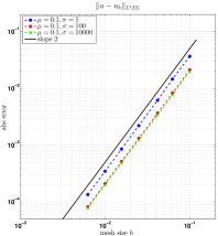
(a)

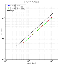
(b)

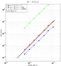
(c)

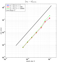
(d)

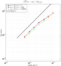
(e)

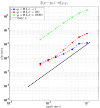
(f)

Figure 4.1: Low-Reynolds-number 2D Taylor Problem with $\mu=0.1$ and $\mathcal{P}^{1}$ approximations: Convergence rates in $L^{2}$-norms for velocity, velocity gradient and pressure in the domain (top row) and on the boundary (bottom row).

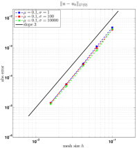
(a)

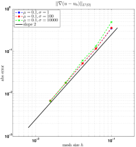
(b)

(c)

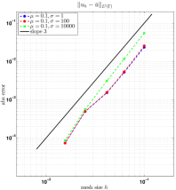
(d)

(e)

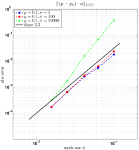
(f)

Figure 4.2: Low-Reynolds-number 2D Taylor Problem with $\mu=0.1$ and $\mathcal{P}^{2}$ approximations: Convergence rates in $L^{2}$-norms for velocity, velocity gradient and pressure in the domain (top row) and on the boundary (bottom row).

4.1.2 Convection dominant flow

The same studies are carried out for convection dominant flow with $\mu=0.0001$. In this setting, the resulting Oseen system exhibits highly varying element Reynolds numbers $\operatorname{Re}_{T}$ due to the locally dominating advective term $\boldsymbol{\beta}\cdot\nabla\boldsymbol{u}$. In contrast to the previous studies, the full stabilization parameter scalings in $\phi_{u},\phi_{\beta},\phi_{p}$ including advective and reactive contributions, see (3.10), are now required for all continuous interior penalty and related ghost-penalty stabilizations as well as for the mass conservation boundary term to ensure inf-sup stability and optimality of the error convergence. In Fig. 4.3 and Fig. 4.4 errors are reported for the same family of triangulations as for the viscous setting. While the velocity approximations again show optimality in the domain and on the boundary, for the pressure we obtain convergence of order $k+1$, which confirms the potential gain of half an order compared to the viscous flow regime, similar to observations made in [1].

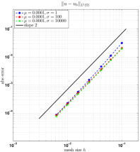
(a)

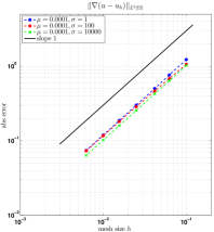
(b)

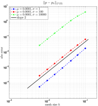
(c)

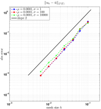
(d)

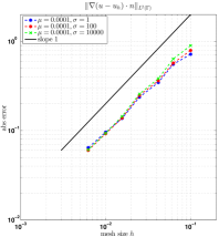
(e)

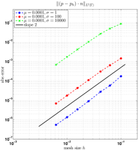
(f)

Figure 4.3: High-Reynolds-number 2D Taylor Problem with $\mu=0.0001$ and $\mathcal{P}^{1}$ approximations: Convergence rates in $L^{2}$-norms for velocity, velocity gradient and pressure in the domain (top row) and on the boundary (bottom row).

(a)

(b)

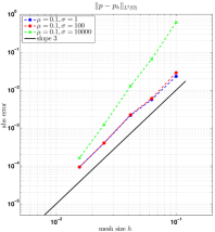
(c)

(d)

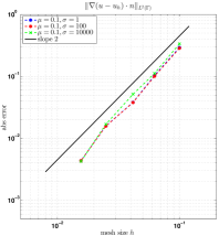
(e)

(f)

Figure 4.4: High-Reynolds-number 2D Taylor Problem with $\mu=0.0001$ and $\mathcal{P}^{2}$ approximations: Convergence rates in $L^{2}$-norms for velocity, velocity gradient and pressure in the domain (top row) and on the boundary (bottom row).

4.2 Convergence Study - 3D Beltrami Flow

To support the theoretical results also in three spatial dimensions, we consider the well-studied Beltrami-flow example, see, e.g, in [44, 1]. The steady Beltrami flow is analytically given as

$$u_{1}(x_{1},x_{2},x_{3}) =be^{a(x_{1}-x_{3})+b(x_{2}-x_{3})}-ae^{a(x_{3}-x_{2})+b(x_{1}-x_{2})},$$ (4.5)

$$u_{2}(x_{1},x_{2},x_{3}) =be^{a(x_{2}-x_{1})+b(x_{3}-x_{1})}-ae^{a(x_{1}-x_{3})+b(x_{2}-x_{3})},$$ (4.6)

$$u_{3}(x_{1},x_{2},x_{3}) =be^{a(x_{3}-x_{2})+b(x_{1}-x_{2})}-ae^{a(x_{2}-x_{1})+b(x_{3}-x_{1})},$$ (4.7)

$$p(x_{1},x_{2},x_{3}) =(a^{2}+b^{2}+ab)[e^{a(x_{1}-x_{2})+b(x_{1}-x_{3})}+e^{a(x_{2}-x_{3})+b(x_{2}-x_{1})}+e^{a(x_{3}-x_{1})+b(x_{3}-x_{2})}]$$ (4.8)

with $a=b=\pi/4$. The velocity field $\boldsymbol{u}$ is solenoidal by construction. The right-hand side $\boldsymbol{f}$ and the boundary data $\boldsymbol{g}$ are adapted to the Oseen problem (2.1)–(2.3) accordingly.

Numerical solutions are computed on a spherical fluid domain with radius $r=0.45$, given implicitly as

$$\Omega=\left\{\boldsymbol{x}\in\mathbb{R}^{3}\leavevmode\nobreak\ |\leavevmode\nobreak\ \phi(x_{1},x_{2},x_{3})=\sqrt{(x_{1}-1.0)^{2}+(x_{2}-0.5)^{2}+(x_{3}-0.5)^{2}}-0.45<0\right\},$$ (4.9)

where its center is located at $(1.0,0.5,0.5)$. The level-set field $\phi$ and the solutions are approximated on the active parts of a family of background meshes $\widehat{\mathcal{T}}_{h}$ covering a background cube $[0.5,1.5]\times[0,1]^{2}$ . Thereby, each mesh is constructed of $N^{3}$ cubes, where each cube is subdivided into six tetrahedra $\mathcal{P}^{1}(T)$. Here, $N$ denotes the number of cubes in each coordinate direction and $h=1/N$ is the short length of each tetrahedra $T$. Similar to the two-dimensional setting, a low- and a high-Reynolds-number setting is considered, characterized by two different viscosities $\mu=0.1$ and $\mu=0.0001$. Computed velocity and pressure approximation errors $(\boldsymbol{u}_{h}-\boldsymbol{u})$ and $(p_{h}-p)$ are shown in Fig. 4.5 for the low-Reynolds-number case and in Fig. 4.6 for the high-Reynolds-number case. The same optimal rates for velocity errors as well as super-convergence for the pressure can be observed similar to the two-dimensional example.

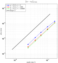
(a)

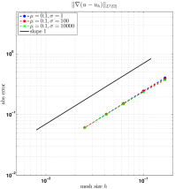
(b)

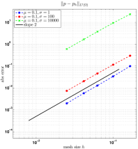
(c)

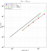
(d)

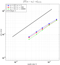
(e)

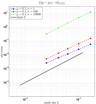
(f)

Figure 4.5: Low-Reynolds-number 3D Beltrami Flow with $\mu=0.1$: Convergence rates in $L^{2}$-norms for velocity, velocity gradient and pressure in the domain (top row) and on the boundary (bottom row).

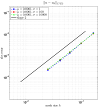
(a)

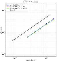
(b)

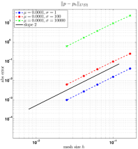
(c)

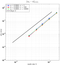
(d)

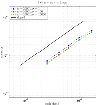
(e)

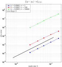
(f)

Figure 4.6: High-Reynolds-number 3D Beltrami Flow with $\mu=0.0001$: Convergence rates in $L^{2}$-norms for velocity, velocity gradient and pressure in the domain (top row) and on the boundary (bottom row).

To underline the stability of the velocity and pressure solutions for the high-Reynolds-number setting, in Fig. 4.7, velocity streamlines and the pressure solution are visualized along cross-sections computed on a coarse non-boundary-fitted mesh. It is clearly visible that the solutions do not exhibit any oscillatory behavior, neither in the interior of the domain, nor at the boundary. This is due to the different proposed continuous interior penalty and ghost-penalty stabilizations. This fact underlines the stability of our proposed formulation even though the solution exhibits highly varying local element Reynolds numbers in the computational domain.

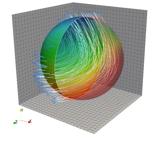
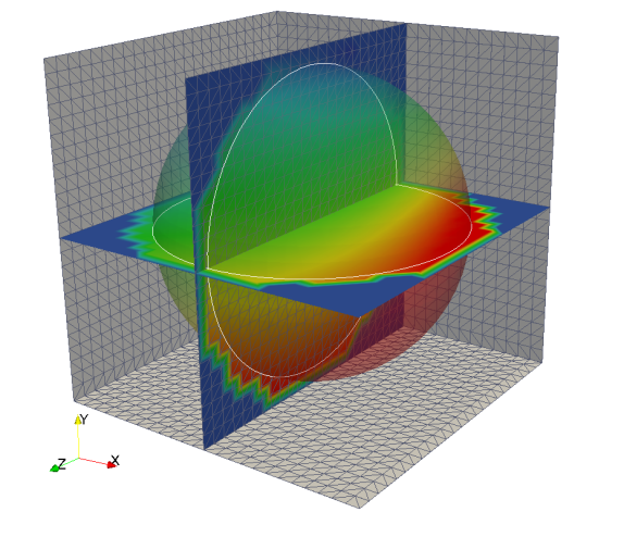
Figure 4.7: High-Reynolds-number 3D Beltrami flow: Computed velocity and pressure solutions on unfitted mesh with $h=1/24$. Stable solutions in the interior of the domain and in the boundary zone due to sufficient control ensured by different CIP and GP stabilization terms. Left: Streamlines colored by velocity magnitude and half-sphere ($x_{1}<1.0$) colored by pressure distribution. Right: Pressure solution at cross-sections defined by $x_{1}=1.0$ and $x_{2}=0.5$.

4.3 Flow through a Helical Pipe

In the final numerical experiment, we demonstrate the applicability of the proposed cut finite element formulation to solve the full time-dependent incompressible Navier-Stokes equations in a complicated, implicitly described domain. Temporal discretization is based on a one-step-$\theta$ scheme and the non-linear convective term is approximated by fixed-point iterations. The resulting series of linear Oseen type systems are solved by the proposed cut finite element method.

In this example, we consider the incompressible flow through a helical pipe. The relevance of curved pipe flows ranges from basic industrial applications like chemical reactors, heat exchangers and pipelines to medical applications considering physiological flows in the human body. Helical pipe flows have been extensively studied in literature, see, e.g., in [45, 46, 47].

The geometric setup of the pipe considered in this work is depicted in Fig. 4.8 and is described as follows:

(a)

(b)

Figure 4.8: Helical Pipe Flow at $\operatorname{Re}=100$: (a) Flow during the ramp phase at $t=0.5$. (b) Laminar flow including twisted streamlines at $t=3.0$ when flow reaches steady state. Streamlines start at inflow boundary located in a radius of $0.04$ around pipe centerline and are colored by velocity magnitude at $t=0.5$ and by vorticity at $t=3.0$. Pressure distribution is visualized along pipe surface.

The cross-section of the pipe defines a circle with a radius $r=0.1$ which is expanded along a helical curve parametrized by $\boldsymbol{x}_{\textrm{curv}}(s)=(R\cos(2\pi s),R\sin(2\pi s),\alpha s)$. This three-dimensional curve turns around the $x_{3}$-axis at a constant distance of $R=0.2$ and a constant thread pitch of $\alpha=0.6$. The spiral twists four times parametrized by $s\in[-2,2]$. In addition, a cylinder with a radius equal to the cross-section radius $r$ and a length of $h=0.35$ is put on the lower end of the spiral. Its orientation is aligned to the tangential vector $\boldsymbol{t}(s)=\partial\boldsymbol{x}_{\textrm{curv}}(s)/\partial s$ of the helix at $s=-2$.

The front end of the cylinder defines the inflow boundary $\Gamma_{\mathrm{in}}$, where a velocity $\boldsymbol{g}=u_{\textrm{in}}\boldsymbol{n}$ is imposed where $\boldsymbol{n}=\boldsymbol{t}(s=-2)$ denotes the unit vector which is normal to the cylinder cross section. Along the cylindrical and helical pipe surfaces, zero boundary conditions $\boldsymbol{g}=\boldsymbol{0}$ are imposed, while at the back end of the helical pipe a zero-traction Neumann boundary condition is set. As before, all boundary conditions are enforced weakly.

The geometry as well as the flow solution are approximated on a cut background mesh $\widehat{\mathcal{T}}_{h}$ covering a background cuboid $[-0.4,0.4]\times[-0.4,0.4]\times[-1.5,1.5]$ with $76\times 76\times 285$ trilinearly interpolated hexahedral elements. In total, the number of active velocity and pressure degrees of freedom is $859612$.

In the following, we consider a laminar pipe flow at $\operatorname{Re}=100$, where the characteristic Reynolds number is defined as $\operatorname{Re}=u_{\textrm{eff}}r/\mu$ with an effective cross-section averaged velocity $u_{\textrm{eff}}$, the pipe radius $r$ and the viscosity of the fluid $\mu$. At the inflow a constant velocity of $u_{\textrm{in}}=u_{\textrm{eff}}=3.8$ is imposed which drives the mass flow. Thereby, the velocity is chosen according to a wall Reynolds number of $\operatorname{Re}_{\tau}=180$ for pipe flows, see, e.g., in [48] for further explanations. For this setup the viscosity is $\mu=1.9\cdot 10^{-3}$. The pipe flow is investigated for a total simulation time of $T_{\textrm{end}}=3$ which is the approximated time needed for $3$ runs through the whole pipe along its centerline. For the temporal discretization a one-step-$\theta$ scheme with $\theta=0.5$ is applied and the time-step length is set to $\Delta t=0.001$, which ensures a maximum $\operatorname{CFL}$-number $<0.5$. The inflow velocity is increased within $t\in[0,T_{1}]$ by a ramp function $1/2(1-\cos(\pi t/T_{1}))$ with $T_{1}=0.1$.

In Fig. 4.8, the solution to the pipe flow is shown during the ramp phase at $t=0.5$ and when the flow is fully developed and reached steady state, as expected for this laminar setting. During the ramp phase, when the flow enters the helical pipe, streamlines follow the helical main curve through the pipe. During the first turn the distance of the line of highest velocities to the $x_{3}$-axis decreases it’s initial value $R$, however, remains unchanged for all following turns. A snapshot of the ramp phase including streamlines and pressure distribution along the pipe surface is shown in Fig. 4.8a. Contour lines of the velocity magnitude at a cross-section clip plane $x_{2}=0.0$ is shown in Fig. 4.9a for the pipe range of $s\in[0,1.5]$. Pressure isocontours along the pipe surface are visualized in Fig. 4.9b. Accurate enforcement of the zero boundary condition along the pipe surface as well as stability of velocity and pressure solutions are clearly visible.

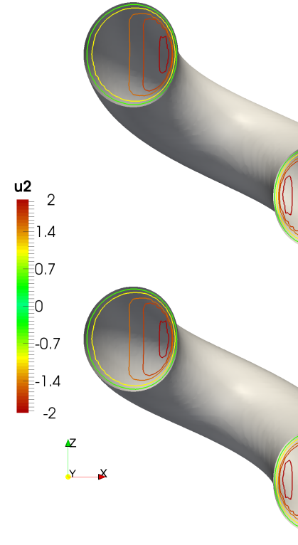
(a)

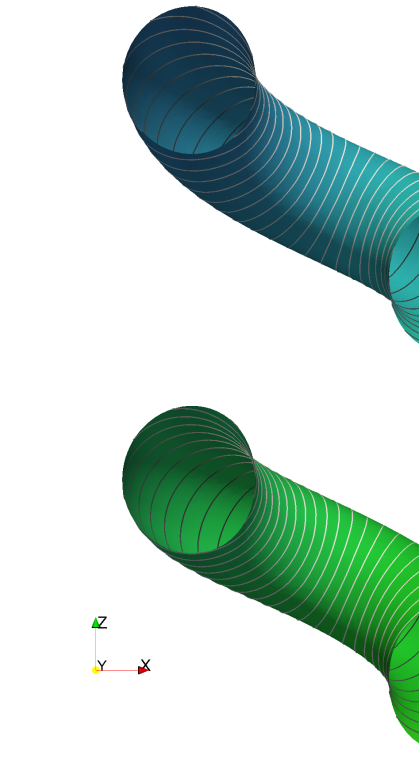
(b)

Figure 4.9: Helical Pipe Flow at $\operatorname{Re}=100$ at $t=0.5$: (a) Isocontours of velocity magnitude at a cross section defined by the clip plane $x_{2}=0.0$ for a helix range of $s\in[0,1.5]$ show higher velocities with decreasing distance to the $x_{3}$-axis due to higher mass flow rate. Zero boundary condition at the helix surface is accurately enforced and velocity solution is stable in the interior of the fluid domain as well as near the boundary. (b) Pressure contour lines at the helix surface show a stable pressure solution near the boundary.

When the flow is fully developed the flow pattern clearly changes and streamlines are twisted. However, the flow reaches steady state after some time, which is shown in a snapshot in Fig. 4.8b at $t=3.0$ including streamlines colored by vorticity and the pressure distribution is depicted along the helical surface. It is inherently linked to the weak enforcement technique that the enforcement of boundary conditions in wall tangential direction gets relaxed for higher local Reynolds numbers near the boundary. However, the non-penetration condition in wall normal direction of the pipe is still sufficiently enforced. Moreover, the solution exhibits non-oscillatory stable velocity and pressure due to stabilizing effects of the different proposed stabilization operators in the interior of the fluid domain as well as near the boundary zone. Contour lines are visualized in Fig. 4.10a for the velocity and in Fig. 4.10b for the pressure.

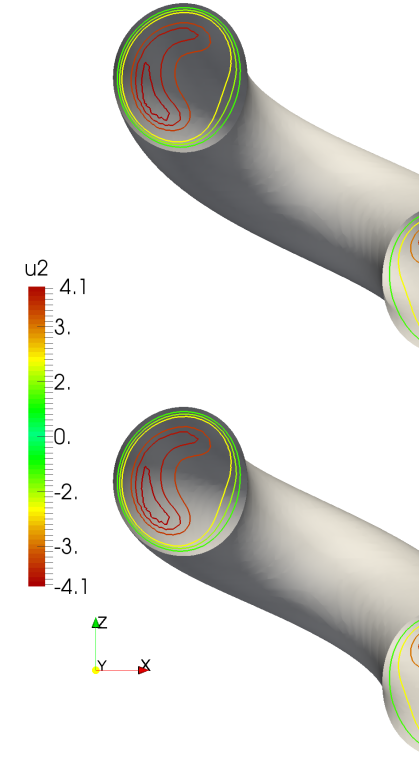
(a)

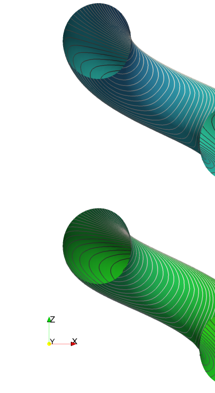
(b)

Figure 4.10: Helical Pipe Flow at $\operatorname{Re}=100$ at $t=3.0$ when flow reaches steady state: (a) Isocontours of velocity magnitude at a cross section defined by the clip plane $x_{2}=0.0$ for a helix range of $s\in[0,1.5]$ exhibits stable velocity solution in the interior of the fluid domain as well as near the boundary. (b) Pressure contour lines at the helix surface show a stable pressure solution near the boundary.

5 Useful Inequalities and Interpolation Estimates

In this section, we start with the numerical analysis of the proposed cut finite element method (3.22). We collect a number of useful inequalities and elucidate the role of the ghost-penalties for the cut finite element method. Moreover, we introduce suitable interpolation operators which will be instrumental in deriving stability bounds in Section 6 and a priori error estimates in Section 7.

5.1 Assumption on the Mesh and the Velocity Field

To simplify the presentation of the numerical analysis of our cut finite element method, we assume quasi-uniform meshes. However, the subsequent analysis can be also adapted to the case of locally quasi-uniform meshes, as considered for boundary-fitted meshes in Burman et al. [1]. Recall that the velocity field $\boldsymbol{\beta}$ satisfies $\boldsymbol{\beta}\in[W^{1,\infty}(\Omega)]^{d}\subseteq[C^{0,1}(\Omega)]^{d}$ by assumption and thus there is a piecewise constant discrete vector field $\boldsymbol{\beta}_{h}$ satisfying

$$h^{\frac{1}{2}}\|\boldsymbol{\beta}-\boldsymbol{\beta}_{h}\|_{0,\infty,\partial T}+\|\boldsymbol{\beta}-\boldsymbol{\beta}_{h}\|_{0,\infty,T}\lesssim h\|\boldsymbol{\beta}\|_{1,\infty,T}\quad\text{and}\quad\|\boldsymbol{\beta}_{h}\|_{0,\infty,T}\lesssim\|\boldsymbol{\beta}\|_{0,\infty,T}\quad\forall\,T\in\mathcal{T}_{h}.$$ (5.1)

Such an approximative vector field $\boldsymbol{\beta}_{h}$ will be used at several occasions in the forthcoming numerical analysis. As usual, the notation $a\lesssim b$ means that $a\leqslant Cb$ for a generic positive constant $C$ which is independent of $h$. Similar to [1], we additionally require that the flow field $\boldsymbol{\beta}$ is sufficiently resolved by the mesh in the sense that for some constant $c_{\beta}>1$ and $\forall\,T\in\mathcal{T}_{h}$

$$c_{\beta}^{-1}\|\boldsymbol{\beta}\|_{0,\infty,T^{\prime}}\leqslant\|\boldsymbol{\beta}\|_{0,\infty,T}\leqslant c_{\beta}\|\boldsymbol{\beta}\|_{0,\infty,T^{\prime}}\quad\forall\,T^{\prime}\in\omega(T),$$ (5.2)

where $\omega(T)$ denotes a local patch of elements neighboring $T$. Assumption (5.2) can be ensured if, e.g.,

$$\|\boldsymbol{\beta}\|_{1,\infty,\omega(T)}\leqslant d_{\beta}h^{-1}\|\boldsymbol{\beta}\|_{0,\infty,\omega(T)}\quad\forall\,T\in\mathcal{T}_{h}$$ (5.3)

is satisfied for some constant $0<d_{\beta}<h/\operatorname{diam}(\omega(T))=:c_{\omega}$. Then

$$\|\boldsymbol{\beta}\|_{0,\infty,\omega(T)} \leqslant\|\boldsymbol{\beta}\|_{0,\infty,T^{\prime}}+\operatorname{diam}(\omega(T))\|\boldsymbol{\beta}\|_{1,\infty,\omega(T)}\leqslant\|\boldsymbol{\beta}\|_{0,\infty,T^{\prime}}+c_{\omega}^{-1}d_{\beta}\|\boldsymbol{\beta}\|_{0,\infty,\omega(T)}$$ (5.4)

and consequently, assumption (5.2) holds with $c_{\beta}^{-1}=1-c_{\omega}^{-1}d_{\beta}$ since for any $T,T^{\prime}\in\omega(T)$

$$(1-c_{\omega}^{-1}d_{\beta})\|\boldsymbol{\beta}\|_{0,\infty,T}\leqslant(1-c_{\omega}^{-1}d_{\beta})\|\boldsymbol{\beta}\|_{0,\infty,\omega(T)}\leqslant\|\boldsymbol{\beta}\|_{0,\infty,T^{\prime}}.$$ (5.5)

Due to assumption (5.2), the piecewise constant stabilization parameters are comparable in the sense that for $\phi\in\{\phi_{u},\phi_{\beta},\phi_{p}\}$

$$(c_{\beta}c_{\mathcal{T}_{h}})^{-1}\phi_{T^{\prime}}\leqslant\ \phi_{T}\leqslant\ (c_{\beta}c_{\mathcal{T}_{h}})\phi_{T^{\prime}}\quad\forall\,T^{\prime}\in\omega(T),$$ (5.6)

where $c_{\mathcal{T}_{h}}$ characterizes the quasi-uniformness of $\mathcal{T}_{h}$. With this in mind, we will simply write

$$\phi_{T}\sim\phi_{T^{\prime}}\quad\forall T^{\prime}\in\omega(T),\qquad\phi_{F}\sim\phi_{T}\quad\forall T\in\omega(F).$$ (5.7)

5.2 Trace Inequalities and Inverse Estimates

Throughout our analysis, we will make heavy use of the following well-known generalized inverse and trace inequalities for discrete functions $v_{h}\in\mathcal{X}_{h}$:

$$\|D^{j}v_{h}\|_{T} \lesssim h^{i-j}\|D^{i}v_{h}\|_{T} \quad\forall\,T\in\mathcal{T}_{h},\quad 0\leqslant i\leqslant j,$$ (5.8)

$$\|\partial_{\boldsymbol{n}}^{j}v_{h}\|_{\partial T} \lesssim h^{i-j-1/2}\|D^{i}v_{h}\|_{T} \quad\forall\,T\in\mathcal{T}_{h},\quad 0\leqslant i\leqslant j,$$ (5.9)

and their counterpart for elements $$T \Gamma$$ which are arbitrarily intersected by the boundary

$$\|\partial_{\boldsymbol{n}}^{j}v_{h}\|_{\Gamma\cap T} \lesssim h^{i-j-1/2}\|D^{i}v_{h}\|_{T} \quad\forall\,T\in\mathcal{T}_{h},\quad 0\leqslant i\leqslant j,$$ (5.10)

proven in [32, BurmanHansboLarsonEtAl2016]. Here and throughout this work, we use the notation $a\lesssim b$ for $a\leqslant Cb$ for some generic positive constant $C$ which varies with the context but is always independent of the mesh size $h$ and the position of $\Gamma$ relative to $\mathcal{T}_{h}$. For $v\in H^{1}(\Omega^{\ast}_{h})$, we will make use of trace inequalities of the form

$$\|v\|_{\partial T} \lesssim h^{-1/2}\|v\|_{T}+h^{1/2}\|\nabla v\|_{T}\quad\forall\,T\in\mathcal{T}_{h},$$ (5.11)

$$\|v\|_{\Gamma\cap T} \lesssim h^{-1/2}\|v\|_{T}+h^{1/2}\|\nabla v\|_{T}\quad\forall\,T\in\mathcal{T}_{h},$$ (5.12)

see [32, BurmanHansboLarsonEtAl2016] for a proof of the second one. Finally, we recall the well-known Poincaré and Korn inequalities [49], stating that $\forall\,\boldsymbol{v}\in[H_{0}^{1}(\Omega)]^{d}$,

$$\|\boldsymbol{v}\|_{0,\Omega} \lesssim C_{P}\|\nabla\boldsymbol{v}\|_{0,\Omega},$$ (5.13)

$$\|\nabla\boldsymbol{v}\|_{0,\Omega} \lesssim\|{\boldsymbol{\epsilon}}(\boldsymbol{v})\|_{0,\Omega},$$ (5.14)

and the following variants if the boundary trace of $\boldsymbol{v}$ is not vanishing, that is $\forall\,\boldsymbol{v}\in[H^{1}(\Omega)]^{d}$:

$$\|\boldsymbol{v}\|_{0,\Omega} \lesssim C_{P}(\|\nabla\boldsymbol{v}\|_{0,\Omega}+\|\boldsymbol{v}\|_{\Gamma}),$$ (5.15)

$$\|\boldsymbol{v}\|_{1,\Omega} \lesssim\|{\boldsymbol{\epsilon}}(\boldsymbol{v})\|_{0,\Omega}+\|\boldsymbol{v}\|_{0,\Omega},$$ (5.16)

$$\|\boldsymbol{v}\|_{1,\Omega} \lesssim\|{\boldsymbol{\epsilon}}(\boldsymbol{v})\|_{0,\Omega}+\|\boldsymbol{v}\|_{0,\Gamma}.$$ (5.17)

5.3 Interpolation Operators

To construct an appropriate interpolation operator $L^{2}(\Omega)\to\mathcal{X}_{h}$, we first recall that for the Sobolev spaces $W^{m,q}(\Omega)$, $0\leqslant m<\infty$, $1\leqslant q\leqslant\infty$, an extension operator can be defined

$$E:W^{m,q}({\Omega})\rightarrow W^{m,q}(\Omega^{\ast})$$ (5.18)

which is bounded

$$\|Ev\|_{m,q,\Omega^{\ast}}\lesssim\|v\|_{m,q,\Omega},$$ (5.19)

see [50] for a proof. Occasionally, we write $v^{\ast}=Ev$. Choosing some fixed Lipschitz-domain $\Omega^{\ast}$ such that $\Omega^{\ast}_{h}\subset\Omega^{\ast}$ for $h\lesssim 1$, we can define for any interpolation operator $\pi_{h}:H^{s}(\Omega^{\ast}_{h})\to\mathcal{X}_{h}$ its “fictitious domain” variant $\pi_{h}^{\ast}:H^{s}(\Omega)\to\mathcal{X}_{h}$ by simply requiring that

$$\pi_{h}^{\ast}u=\pi_{h}(u^{\ast})$$ (5.20)

for $u\in H^{s}(\Omega)$. In particular, we choose $\pi_{h}$ to be the Clément operator, see for instance [51]. Recall that for $v\in H^{r}(\Omega^{\ast})$, the following interpolation estimates holds for the Clément interpolant:

$$\|v-\pi_{h}v\|_{s,T} \lesssim h^{t-s}|v|_{t,\omega(T)}, \quad 0\leqslant s\leqslant t\leqslant m\quad \forall\,T\in\mathcal{T}_{h},$$ (5.21)

$$\|v-\pi_{h}v\|_{s,F} \lesssim h^{t-s-1/2}|v|_{t,\omega(F)}, \quad 0\leqslant s\leqslant t-1/2\leqslant m-1/2\quad \forall\,F\in\mathcal{F}_{h},$$ (5.22)

with $s,t\in\mathbb{N}$, $m=\min\{r,k+1\}$ and $k$ the interpolation order of $\mathcal{X}_{h}$. Here, $\omega(T)$ and $\omega(F)$ are the sets of elements in $\mathcal{T}_{h}$ sharing at least one vertex with $T$ and $F$, respectively. Due to the boundedness of the extension operator (5.19), we observe that the extended Clément interpolant $\pi_{h}^{\ast}$ satisfies

$$\|v^{\ast}-\pi_{h}^{\ast}v\|_{s,\mathcal{T}_{h}} \lesssim h^{t-s}\|v\|_{t,\Omega}, \quad 0\leqslant s\leqslant t\leqslant m,$$ (5.23)

$$\|v^{\ast}-\pi_{h}^{\ast}v\|_{s,\mathcal{F}_{h}} \lesssim h^{t-s-1/2}\|v\|_{t,\Omega}, \quad 0\leqslant s\leqslant t-1/2\leqslant m-1/2,$$ (5.24)

where the broken norms $\|\cdot\|_{\mathcal{F}_{h}}$ and $\|\cdot\|_{\mathcal{T}_{h}}$ are defined as in Section 1.1. In particular, we make use of the stability property

$$\|\pi_{h}^{\ast}v\|_{s,\Omega} \lesssim\|v\|_{s,\Omega}, \quad 0\leqslant s\leqslant m.$$ (5.25)

The Clément interpolant is denoted by $\boldsymbol{\pi}_{h}^{\ast}$ for vector-valued functions $\boldsymbol{v}$ and by $\Pi_{h}^{\ast}$ for functions in a product space.

A main ingredient in the analysis of the continuous interior penalty method in [1, 52] is the use of the Oswald interpolation operator. The Oswald interpolation operator defines a mapping $\mathcal{O}_{h}:\mathcal{P}_{\mathrm{dc}}^{k}(\mathcal{T}_{h})\to\mathcal{P}^{\max\{1,k\}}(\mathcal{T}_{h})$, with $\mathcal{P}_{\mathrm{dc}}^{k}(\mathcal{T}_{h})$ and $\mathcal{P}^{k}(\mathcal{T}_{h})$ denoting the space of discontinuous and continuous piecewise polynomials of order $k$. More precisely, for $v\in\mathcal{P}_{\mathrm{dc}}^{k}(\mathcal{T}_{h})$, the function $\mathcal{O}_{h}v$ is constructed in each interpolation node $\boldsymbol{x}_{i}$ by the average value

$$\mathcal{O}_{h}v(\boldsymbol{x}_{i})=\dfrac{1}{\mathrm{card}(\mathcal{T}_{h}(\boldsymbol{x}_{i}))}\sum_{T\in\mathcal{T}_{h}(\boldsymbol{x}_{i})}v|_{T}(\boldsymbol{x}_{i})$$ (5.26)

where $\mathcal{T}_{h}(\boldsymbol{x}_{i})$ is the set of all elements $T\in\mathcal{T}_{h}$ sharing the node $\boldsymbol{x}_{i}$. In particular, it was shown there that for $w_{h}\in\mathcal{X}_{h}^{\mathrm{dc}}=\{v\in L^{2}(\Omega^{\ast}):v|_{T}\in\mathcal{P}^{k}(T)\;\forall\,T\in\mathcal{T}_{h}\}$, the fluctuation $w_{h}-\mathcal{O}_{h}w_{h}$ can be controlled in terms of jump-penalties:

Lemma 5.1.

Let $\phi$ be a piecewise constant function and $w_{h}\in\mathcal{X}_{h}^{\mathrm{dc}}$. Then

$$\|\phi^{\frac{1}{2}}(w_{h}-\mathcal{O}_{h}w_{h})\|_{T}^{2}\lesssim\sum_{F\in\mathcal{F}_{i}(T)}\phi_{T}h\|\llbracket w_{h}\rrbracket\|_{F}^{2}\quad\forall\,w_{h}\in\mathcal{X}_{h}^{\mathrm{dc}},$$ (5.27)

where $\mathcal{F}_{i}(T)$ denotes the set of all faces $F\in\mathcal{F}_{i}$ with $F\cap T\neq\emptyset$, and the hidden constant depends only on the shape-regularity of the mesh, the order of the finite element space $\mathcal{X}_{h}^{\mathrm{dc}}$ and the dimension $d$.

We refer to [52] for a proof. The previous lemma elucidates the role of the CIP stabilization operators (3.6)–(3.8) as a control of certain fluctuations:

Corollary 5.2.

Under the assumptions of Lemma 5.1 it holds that

$$\|\phi_{\beta}^{\frac{1}{2}}(\boldsymbol{\beta}_{h}\cdot\nabla\boldsymbol{v}_{h}-\mathcal{O}_{h}(\boldsymbol{\beta}_{h}\cdot\nabla\boldsymbol{v}_{h}))\|_{T}^{2} \lesssim\sum_{F\in\mathcal{F}_{i}(T)}\phi_{\beta,T}h\|\llbracket\boldsymbol{\beta}_{h}\cdot\nabla\boldsymbol{v}_{h}\rrbracket\|_{F}^{2},$$ (5.28)

$$\|\phi_{p}^{\frac{1}{2}}(\nabla q_{h}-\mathcal{O}_{h}(\nabla q_{h}))\|_{T}^{2} \lesssim\sum_{F\in\mathcal{F}_{i}(T)}\phi_{p,T}h{\|\llbracket\boldsymbol{n}_{F}\cdot\nabla q_{h}\rrbracket\|_{F}^{2}},$$ (5.29)

$$\|\phi_{u}^{\frac{1}{2}}(\nabla\cdot\boldsymbol{v}_{h}-\mathcal{O}_{h}(\nabla\cdot\boldsymbol{v}_{h}))\|_{T}^{2} \lesssim\sum_{F\in\mathcal{F}_{i}(T)}\phi_{u,T}h{\|\llbracket\nabla\cdot\boldsymbol{v}_{h}\rrbracket\|_{F}^{2}}.$$ (5.30)

In the forthcoming stability and a priori error analysis we will make heavy use of certain continuous, piecewise linear versions of the stabilization parameters defined by

$$\widetilde{\phi}=\mathcal{O}_{h}\phi,\quad\phi\in\{\phi_{\beta},\phi_{u},\phi_{p}\}.$$ (5.31)

Then by the definition of the Oswald interpolant and the local comparability of the stabilization parameters (5.7)

$$\widetilde{\phi}|_{T}\sim\phi_{T},\quad\phi\in\{\phi_{\beta},\phi_{u},\phi_{p}\}.$$ (5.32)

We conclude this section by stating and proving a helpful lemma on the quasi-local stability of the Oswald interpolation in certain weighted norms.

Lemma 5.3.

Let $v_{h}\in\mathcal{X}_{h}$ and let $\phi$ be a piecewise constant function defined on $\mathcal{T}_{h}$. Then

$$\|\phi^{\frac{1}{2}}\mathcal{O}_{h}(v_{h})\|_{T} \lesssim\|\phi_{T}^{\frac{1}{2}}v_{h}\|_{\omega(T)}\quad\forall\,T\in\mathcal{T}_{h}.$$ (5.33)

Proof. The proof is a simple consequence of the Lemma (5.27) and the inverse inequality (5.9):

$$\|\phi^{\frac{1}{2}}\mathcal{O}_{h}(v_{h})\|_{T}^{2}=\|\phi^{\frac{1}{2}}v_{h}\|_{T}^{2}+\|\phi^{\frac{1}{2}}(\mathcal{O}_{h}(v_{h})-v_{h})\|_{T}^{2}\lesssim\|\phi^{\frac{1}{2}}v_{h}\|_{T}^{2}+h\|\phi_{T}^{\frac{1}{2}}\llbracket v_{h}\rrbracket\|_{\mathcal{F}_{h}(T)}^{2}\lesssim\|\phi_{T}^{\frac{1}{2}}v_{h}\|_{T}^{2}+\|\phi_{T}^{\frac{1}{2}}v_{h}\|_{\omega(T)}^{2}.$$ (5.34)

5.4 The Role of the Ghost Penalties

Following [1, 30], the naturals norms associated with the discrete variational problem defined for fitted meshes as $A_{h}+S_{h}=L_{h}$ in (3.12)–(3.16), are given by

$$|\mspace{-1.0mu}|\mspace{-1.0mu}|\boldsymbol{u}_{h}|\mspace{-1.0mu}|\mspace{-1.0mu}|^{2} =\|\sigma^{1/2}\boldsymbol{u}_{h}\|_{\Omega}^{2}+\|\mu^{1/2}\nabla\boldsymbol{u}_{h}\|_{\Omega}^{2}+\|(\gamma\mu/h)^{1/2}\boldsymbol{u}_{h}\|^{2}_{\Gamma}+s_{u}(\boldsymbol{u}_{h},\boldsymbol{u}_{h})$$

$$\quad+\||\boldsymbol{\beta}\cdot\boldsymbol{n}|^{1/2}\boldsymbol{u}_{h}\|_{\Gamma}^{2}+\|(\gamma\phi_{u}/h)^{1/2}\boldsymbol{u}_{h}\cdot\boldsymbol{n}\|^{2}_{\Gamma}+s_{\beta}(\boldsymbol{u}_{h},\boldsymbol{u}_{h}),$$ (5.35)

$$|\mspace{-1.0mu}|\mspace{-1.0mu}|p_{h}|\mspace{-1.0mu}|\mspace{-1.0mu}|^{2} =\Phi_{p}\|p_{h}\|_{\Omega}^{2}+s_{p}(p_{h},p_{h}),$$ (5.36)

$$|\mspace{-1.0mu}|\mspace{-1.0mu}|U_{h}|\mspace{-1.0mu}|\mspace{-1.0mu}|^{2} =|\mspace{-1.0mu}|\mspace{-1.0mu}|\boldsymbol{u}_{h}|\mspace{-1.0mu}|\mspace{-1.0mu}|^{2}+|\mspace{-1.0mu}|\mspace{-1.0mu}|p_{h}|\mspace{-1.0mu}|\mspace{-1.0mu}|^{2},$$ (5.37)

with $\Phi_{p}$ defined by (3.29). Using similar norms, inf-sup stability and energy-type error estimates were proven in [1].

The main challenge in developing Nitsche-type fictitious domain methods is now to establish stability and a priori error estimates which are independent of the positioning of the unfitted boundary within the background mesh. The key idea is to add certain (weakly) consistent stabilization terms in the vicinity of the boundary which allow to extend suitable norms for finite element functions from the physical domain $\Omega$ to the entire fictitious domain $\Omega^{\ast}_{h}$. The subsequent lemmas elucidate the role of the different ghost penalties and motivate the definition of the fictitious domain norms from (3.25)–(3.28). The following lemma was proven in [27, 33]:

Lemma 5.4.

Let $\Omega$, $\Omega^{\ast}_{h}$ and $\mathcal{F}_{\Gamma}$ be defined as in Section 3.1. Then for scalar functions $p_{h}\in\mathcal{Q}_{h}$ as well as for vector-valued equivalents $\boldsymbol{u}_{h}\in\mathcal{V}_{h}$ the following estimates hold

$$\|p_{h}\|_{\Omega^{\ast}_{h}}^{2} \lesssim\bigl{(}\|p_{h}\|_{\Omega}^{2}+\sum_{F\in\mathcal{F}_{\Gamma}}\sum_{1\leqslant j\leqslant k}{h^{2j+1}\langle\llbracket\partial_{\boldsymbol{n}}^{j}p_{h}\rrbracket,\llbracket\partial_{\boldsymbol{n}}^{j}p_{h}\rrbracket\rangle_{F}}\bigr{)}\lesssim\|p_{h}\|_{\Omega^{\ast}_{h}}^{2},$$ (5.38)

$$\|\boldsymbol{u}_{h}\|_{\Omega^{\ast}_{h}}^{2} \lesssim\bigl{(}\|\boldsymbol{u}_{h}\|_{\Omega}^{2}+\sum_{F\in\mathcal{F}_{\Gamma}}\sum_{1\leqslant j\leqslant k}{h^{2j+1}\langle\llbracket\partial_{\boldsymbol{n}}^{j}\boldsymbol{u}_{h}\rrbracket,\llbracket\partial_{\boldsymbol{n}}^{j}\boldsymbol{u}_{h}\rrbracket\rangle_{F}}\bigr{)}\lesssim\|\boldsymbol{u}_{h}\|_{\Omega^{\ast}_{h}}^{2},$$ (5.39)

$$\|\nabla\boldsymbol{u}_{h}\|_{\Omega^{\ast}_{h}}^{2} \lesssim\bigl{(}\|\nabla\boldsymbol{u}_{h}\|_{\Omega}^{2}+\sum_{F\in\mathcal{F}_{\Gamma}}\sum_{1\leqslant j\leqslant k}{h^{2j-1}\langle\llbracket\partial_{\boldsymbol{n}}^{j}\boldsymbol{u}_{h}\rrbracket,\llbracket\partial_{\boldsymbol{n}}^{j}\boldsymbol{u}_{h}\rrbracket\rangle_{F}}\bigr{)}\lesssim\|\nabla\boldsymbol{u}_{h}\|_{\Omega^{\ast}_{h}}^{2},$$ (5.40)

where the hidden constants depend only on the shape-regularity and the polynomial order, but not on the mesh or the location of $\Gamma$ within $\mathcal{T}_{h}$.

Thus the role of the ghost-penalties $g_{\mu}$ and $g_{\sigma}$ is to extend the control of the viscous and reactive element contributions in the velocity norm (5.4) from $\Omega$ to the fictitious domain $\Omega_{h}^{\ast}$:

Corollary 5.5.

Let $\Omega$, $\Omega^{\ast}_{h}$ and $\mathcal{F}_{\Gamma}$ be defined as in Section 3.1. Then for $\boldsymbol{u}_{h}\in\mathcal{V}_{h}$ the following scaled estimates hold

$$\|\mu^{\frac{1}{2}}\nabla\boldsymbol{u}_{h}\|_{\Omega^{\ast}_{h}}^{2} \lesssim\|\mu^{\frac{1}{2}}\nabla\boldsymbol{u}_{h}\|_{\Omega}^{2}+g_{\mu}(\boldsymbol{u}_{h},\boldsymbol{u}_{h})\lesssim\|\mu^{\frac{1}{2}}\nabla\boldsymbol{u}_{h}\|_{\Omega^{\ast}_{h}}^{2},$$ (5.41)

$$\|\sigma^{\frac{1}{2}}\boldsymbol{u}_{h}\|_{\Omega^{\ast}_{h}}^{2} \lesssim\|\sigma^{\frac{1}{2}}\boldsymbol{u}_{h}\|_{\Omega}^{2}+g_{\sigma}(\boldsymbol{u}_{h},\boldsymbol{u}_{h})\lesssim\|\sigma^{\frac{1}{2}}\boldsymbol{u}_{h}\|_{\Omega^{\ast}_{h}}^{2},$$ (5.42)

where the ghost-penalty operators $g_{\mu}$ and $g_{\sigma}$ are defined as in (3.20) and (3.21).

One major difference to the numerical analysis proposed by Burman et al. [1] consists in the extended inf-sup stability derived in this work. In [1] inf-sup stability was proven with respect to a weaker semi-norm and the orthogonality and approximation properties of the $L^{2}$ projection were exploited to establish a priori  error estimates. Burman et al. [25] introduced a stabilized, approximate $L^{2}$ projection to facilitate the numerical analysis of a stabilized cut finite element method for the three field Stokes problem based on equal-order, $P_{1}$ elements. The definition of this stabilized $L^{2}$ projection incorporates properly scaled ghost-penalty stabilization and leads to a perturbation of the $L^{2}$ orthogonality in the vicinity of the embedded boundary which is difficult to handle for other than first order elements. To compensate the lack of a suitable CutFEM variant of the $L^{2}$ projection in the subsequent stability analysis, we will gain further control over weakly scaled (semi)-norms

$$\|\phi_{u}^{\frac{1}{2}}\nabla\cdot\boldsymbol{u}_{h}\|_{\Omega^{\ast}_{h}},\quad\|\phi_{\beta}^{\frac{1}{2}}(\boldsymbol{\beta}\cdot\nabla\boldsymbol{u}_{h}+\nabla p_{h})\|_{\Omega^{\ast}_{h}},\quad\|p_{h}\|_{\Omega^{\ast}_{h}}$$ (5.43)

with the help of the CIP stabilization operators $s_{u},s_{\beta},s_{p}$ and their ghost penalty counterparts. Enhancing our natural norms by these residual-based stabilization like contributions allows us to use alternative approximation operators such as the Clément operator for which a proper CutFEM extension can be defined by (5.20).

Remark 5.6.

Previously, Burman2007a established stability and convergence results in related norms for stabilized finite element methods for Friedrich’s systems by demonstrating how to control the relevant $h$-weighted graph-norms using CIP stabilizations. Our approach here was also inspired by the presentation in Knobloch and Tobiska [37], who showed how to gain control over the semi-norm $\|\phi_{\beta}^{\frac{1}{2}}(\boldsymbol{\beta}_{h}\cdot\nabla\boldsymbol{u}_{h}+\nabla p_{h})\|_{\Omega}$ in a local projection stabilized, fitted finite element method for the Oseen problem.

To ensure stability and optimality for cut finite element approximations in the different flow regimes, the semi-norms (5.43) need to be extended to the enlarged domain $\Omega^{\ast}_{h}$ with the help of related ghost-penalty operators $g_{u},g_{\beta},g_{p}$. For this purpose, in the following useful estimates according to the aforementioned norms are derived.

Corollary 5.7.

For $p_{h}\in\mathcal{Q}_{h}$ and $\boldsymbol{u}_{h}\in\mathcal{V}_{h}$ with $\Phi_{p}$ from (3.29), the following estimates hold

$$\Phi_{p}\|p_{h}\|_{\Omega^{\ast}_{h}}^{2} \lesssim\Phi_{p}\|p_{h}\|_{\Omega}^{2}+g_{p}(p_{h},p_{h}),$$ (5.44)

$$\|\phi_{u}^{\frac{1}{2}}\nabla\cdot\boldsymbol{u}_{h}\|_{\Omega^{\ast}_{h}}^{2} \lesssim\|\phi_{u}^{\frac{1}{2}}\nabla\cdot\boldsymbol{u}_{h}\|_{\Omega}^{2}+g_{u}(\boldsymbol{u}_{h},\boldsymbol{u}_{h})$$ (5.45)

where the ghost-penalty operators $g_{p}$ and $g_{u}$ are defined as in (3.18) and (3.19).

Proof. The estimate for the scaled pressure $L^{2}$-norm follows from applying Lemma 5.4 to $\Phi_{p}^{\frac{1}{2}}p_{h}$ and the fact that $\Phi_{p}h^{2}\lesssim\phi_{p,T}\sim\phi_{p,F}$, see definitions (3.29) and (3.10), together with $h\lesssim C_{P}$.

The estimate for the weakly scaled incompressibility results from a localized variant of the ghost-penalty Lemma 5.4, as proven in [33], and the comparability assumption $\phi_{u,T}\sim\phi_{u,T^{\prime}}\sim\phi_{u,F}$ (5.7) on patches of elements $T^{\prime}\in\omega(T)$ surrounding intersected elements $T\in\mathcal{T}_{\Gamma}$. Note that the number of element traversals required to walk from a cut element to an uncut element in a boundary zone patch $\omega(T)$ is bounded independent of $h$ owing to the mesh assumption G3, see Section 3.1.

More subtle is the role of the mixed norm incorporating the advective term and the pressure gradient. Estimates using the ghost-penalty operators $g_{\beta}$ and $g_{p}$ can be deduced as follows.

Lemma 5.8.

Let $\boldsymbol{u}_{h}\in\mathcal{V}_{h}$ and let the scaling functions $\phi_{\beta}$ and $\phi_{p}$ be defined as in (3.10). For a piecewise constant approximation $\boldsymbol{\beta}_{h}\in[\mathcal{X}_{h}^{\mathrm{dc},0}]^{d}$ of $\boldsymbol{\beta}$ on $\mathcal{T}_{h}$ which satisfy the approximation properties specified in (5.1), the following estimate for the streamline diffusion norm holds

$$\|{\phi}_{\beta}^{\frac{1}{2}}(\boldsymbol{\beta}_{h}-\boldsymbol{\beta})\cdot\nabla\boldsymbol{u}_{h}\|_{\Omega^{\ast}_{h}}^{2} \lesssim\omega_{h}\bigl{(}\|\mu^{\frac{1}{2}}\nabla\boldsymbol{u}_{h}\|_{\Omega^{\ast}_{h}}^{2}+\|\sigma^{\frac{1}{2}}\boldsymbol{u}_{h}\|_{\Omega^{\ast}_{h}}^{2}\bigr{)}.$$ (5.46)

The mixed advective-pressure-gradient semi-norm can be estimated as

$$\|\phi_{\beta}^{\frac{1}{2}}(\boldsymbol{\beta}_{h}\cdot\nabla\boldsymbol{u}_{h}+\nabla p_{h})\|_{\Omega^{\ast}_{h}}^{2} \lesssim\|\phi_{\beta}^{\frac{1}{2}}(\boldsymbol{\beta}\cdot\nabla\boldsymbol{u}_{h}+\nabla p_{h})\|_{\Omega}^{2}+g_{\beta}(\boldsymbol{u}_{h},\boldsymbol{u}_{h})+g_{p}(p_{h},p_{h})+\omega_{h}\bigl{(}\|\mu^{\frac{1}{2}}\nabla\boldsymbol{u}_{h}\|_{\Omega^{\ast}_{h}}^{2}+\|\sigma^{\frac{1}{2}}\boldsymbol{u}_{h}\|_{\Omega^{\ast}_{h}}^{2}\bigr{)},$$ (5.47)

with the non-dimensional scaling function $\omega_{h}$ from (3.29).

Proof. 
Estimates (5.46). A simple application of the Cauchy-Schwarz inequality shows that

$$\|{\phi}_{\beta}^{\frac{1}{2}}(\boldsymbol{\beta}_{h}-\boldsymbol{\beta})\cdot\nabla\boldsymbol{u}_{h}\|^{2}_{\Omega^{\ast}_{h}}\lesssim\sum\nolimits_{T\in\mathcal{T}_{h}}\phi_{\beta}\|\boldsymbol{\beta}_{h}-\boldsymbol{\beta}\|_{0,\infty,T}^{2}\|\nabla\boldsymbol{u}_{h}\|^{2}_{T}.$$ (5.48)

Now using the interpolation property of $\boldsymbol{\beta}_{h}$ (5.1) and the simple fact that $\phi_{\beta}\|\boldsymbol{\beta}\|_{0,\infty,T}\lesssim h$ (see definition (3.10)), it can be further estimated that

$$\phi_{\beta}\|\boldsymbol{\beta}_{h}-\boldsymbol{\beta}\|_{0,\infty,T}^{2} \lesssim\phi_{\beta}\|\boldsymbol{\beta}\|_{0,\infty,T}h|\boldsymbol{\beta}|_{1,\infty,T}\lesssim h^{2}|\boldsymbol{\beta}|_{1,\infty,T}.$$ (5.49)

Then we apply the inverse inequality (5.8) to obtain the following simple estimate for $\|\nabla\boldsymbol{u}_{h}\|_{T}$,

$$\|\nabla\boldsymbol{u}_{h}\|_{T}=\dfrac{\mu+\sigma h^{2}}{\mu+\sigma h^{2}}\|\nabla\boldsymbol{u}_{h}\|_{T}^{2}\lesssim\dfrac{1}{\mu+\sigma h^{2}}(\|\mu^{\frac{1}{2}}\nabla\boldsymbol{u}_{h}\|_{T}^{2}+\|\sigma^{\frac{1}{2}}\boldsymbol{u}_{h}\|_{T}^{2}),$$ (5.50)

which gives the desired estimate by taking the maximum over all elements and by defining $\omega_{h}$ as in (3.29).

Estimate (5.47). Note that the function $\boldsymbol{v}_{h}:=\phi_{\beta}(\boldsymbol{\beta}_{h}\cdot\nabla\boldsymbol{u}_{h}+\nabla p_{h})$ is a piecewise polynomial function of order $k-1$ owing to the fact that $\phi_{\beta}$ and $\boldsymbol{\beta}_{h}$ are piecewise constant. Applying the norm equivalence from Lemma 5.4 to $\boldsymbol{v}_{h}$ and using that $\phi_{\beta}\sim\phi_{p}$, as assumed in (3.10), and the local comparability of $\phi$ (5.7) yields

$$\|\phi_{\beta}^{\frac{1}{2}}(\boldsymbol{\beta}_{h}\cdot\nabla\boldsymbol{u}_{h}+\nabla p_{h})\|^{2}_{\Omega^{\ast}_{h}}$$

$$\quad\lesssim\|\phi_{\beta}^{\frac{1}{2}}(\boldsymbol{\beta}_{h}\cdot\nabla\boldsymbol{u}_{h}+\nabla p_{h})\|^{2}_{\Omega}+\sum\nolimits_{j=0}^{k-1}\phi_{\beta,F}h^{2j+1}\|\llbracket\partial_{\boldsymbol{n}}^{j}(\boldsymbol{\beta}_{h}\cdot\nabla\boldsymbol{u}_{h}+\nabla p_{h})\rrbracket\|_{\mathcal{F}_{\Gamma}}^{2}$$ (5.51)

$$\quad\lesssim\|\phi_{\beta}^{\frac{1}{2}}(\boldsymbol{\beta}_{h}\cdot\nabla\boldsymbol{u}_{h}+\nabla p_{h})\|^{2}_{\Omega}+\sum\nolimits_{j=0}^{k-1}\phi_{\beta,F}h^{2j+1}\|\llbracket\partial_{\boldsymbol{n}}^{j}\nabla p_{h}\rrbracket\|_{\mathcal{F}_{\Gamma}}^{2}+\sum\nolimits_{j=0}^{k-1}\phi_{\beta,F}h^{2j+1}\|\llbracket\boldsymbol{\beta}_{h}\cdot\nabla\partial_{\boldsymbol{n}}^{j}\boldsymbol{u}_{h}\rrbracket\|_{\mathcal{F}_{\Gamma}}^{2}$$ (5.52)

$$\quad\lesssim\|\phi_{\beta}^{\frac{1}{2}}(\boldsymbol{\beta}_{h}\cdot\nabla\boldsymbol{u}_{h}+\nabla p_{h})\|^{2}_{\Omega}+\sum\nolimits_{j=0}^{k-1}\phi_{\beta,F}h^{2j+1}\|\llbracket\partial_{\boldsymbol{n}}^{j}\nabla p_{h}\rrbracket\|_{\mathcal{F}_{\Gamma}}^{2}$$

$$\quad\qquad+\sum\nolimits_{j=0}^{k-1}\phi_{\beta,F}h^{2j+1}\|\llbracket(\boldsymbol{\beta}_{h}-\boldsymbol{\beta})\cdot\nabla\partial_{\boldsymbol{n}}^{j}\boldsymbol{u}_{h}\rrbracket\|_{\mathcal{F}_{\Gamma}}^{2}+\sum\nolimits_{j=0}^{k-1}\phi_{\beta,F}h^{2j+1}\|\llbracket\boldsymbol{\beta}\cdot\nabla\partial_{\boldsymbol{n}}^{j}\boldsymbol{u}_{h}\rrbracket\|_{\mathcal{F}_{\Gamma}}^{2}$$ (5.53)

$$\quad\lesssim\|\phi_{\beta}^{\frac{1}{2}}(\boldsymbol{\beta}_{h}\cdot\nabla\boldsymbol{u}_{h}+\nabla p_{h})\|^{2}_{\Omega}+g_{\beta}(\boldsymbol{u}_{h},\boldsymbol{u}_{h})+g_{p}(p_{h},p_{h})+\omega_{h}\bigl{(}\|\mu^{\frac{1}{2}}\nabla\boldsymbol{u}_{h}\|_{\Omega^{\ast}_{h}}^{2}+\|\sigma^{\frac{1}{2}}\boldsymbol{u}_{h}\|_{\Omega^{\ast}_{h}}^{2}\bigr{)}.$$ (5.54)

Here, in the last step, the gradient $\nabla p_{h}=(\partial_{\boldsymbol{n}}p_{h})\boldsymbol{n}_{F}+\boldsymbol{P}_{F}\nabla p_{h}$ has been decomposed into its normal and tangential gradient part using the tangential projection $\boldsymbol{P}_{F}:=\boldsymbol{I}-\boldsymbol{n}_{F}\otimes\boldsymbol{n}_{F}$ and the inverse estimate

$$\|\llbracket\boldsymbol{P}_{F}\nabla\partial_{\boldsymbol{n}}^{j}p_{h}\rrbracket\|_{F}^{2}=\|\boldsymbol{P}_{F}\nabla\llbracket\partial_{\boldsymbol{n}}^{j}p_{h}\rrbracket\|_{F}^{2}\lesssim h^{-2}\|\llbracket\partial_{\boldsymbol{n}}^{j}p_{h}\rrbracket\|_{F}^{2}$$ (5.55)

has been employed on the tangential part to obtain

$$h^{2j+1}\|\llbracket\partial_{\boldsymbol{n}}^{j}\nabla p_{h}\rrbracket\|_{F}^{2}\lesssim h^{2j+1}\|\llbracket\partial_{\boldsymbol{n}}^{j+1}p_{h}\rrbracket\|_{F}^{2}+h^{2j-1}\|\llbracket\partial_{\boldsymbol{n}}^{j}p_{h}\rrbracket\|_{F}^{2}.$$ (5.56)

Choosing the stabilization parameters $\gamma_{\beta},\gamma_{p}>0$ strictly positive allows to control the facet terms in the vicinity of $\Gamma$ by the two higher-order ghost penalty terms $g_{\beta}$ and $g_{p}$. For the facet term which includes the difference $\boldsymbol{\beta}_{h}-\boldsymbol{\beta}$, applying Cauchy Schwarz on the facet followed by the interpolation estimate (5.1) and standard inverse estimates for the remaining normal derivatives of $\boldsymbol{u}_{h}$, which completes the proof of (5.47).

The previous lemma in combination with Corollary 5.5 explains how the ghost penalty terms help us to extend the mixed advective-pressure-gradient semi-norm from the physical domain to the entire active background mesh:

Corollary 5.9.

Under the assumption of Lemma 5.8 it holds that

$$\|\phi_{\beta}^{\frac{1}{2}}(\boldsymbol{\beta}\cdot\nabla\boldsymbol{u}_{h}+\nabla p_{h})\|^{2}_{\Omega^{\ast}_{h}}\lesssim\|\phi_{\beta}^{\frac{1}{2}}(\boldsymbol{\beta}\cdot\nabla\boldsymbol{u}_{h}+\nabla p_{h})\|^{2}_{\Omega}+\omega_{h}|U_{h}|_{h}^{2}.$$ (5.57)

Finally, following up on Remark 3.4, we present a short proof showing how the convective and divergence related ghost penalties (3.17) and (3.18) can be simplified and replaced by the simple ghost-penalty form $\overline{g}_{\beta}$ (3.24).

Lemma 5.10.

Let $\boldsymbol{u}_{h}\in\mathcal{V}_{h}$ and define $\overline{\phi}_{\beta}:=\|\boldsymbol{\beta}\|_{0,\infty,F}^{2}\phi_{\beta}$. Then

$$g_{\beta}(\boldsymbol{u}_{h},\boldsymbol{u}_{h}) \lesssim\gamma_{\beta}\sum_{F\in\mathcal{F}_{\Gamma}}\sum_{1\leqslant j\leqslant k}\overline{\phi}_{\beta}h^{2j-1}(\llbracket\partial_{\boldsymbol{n}}^{j}\boldsymbol{u}_{h}\rrbracket,\llbracket\partial_{\boldsymbol{n}}^{j}\boldsymbol{u}_{h}\rrbracket)_{F},$$ (5.58)

$$g_{u}(\boldsymbol{u}_{h},\boldsymbol{u}_{h}) \lesssim\gamma_{u}\sum_{F\in\mathcal{F}_{\Gamma}}\sum_{1\leqslant j\leqslant k}\overline{\phi}_{\beta}h^{2j-1}(\llbracket\partial_{\boldsymbol{n}}^{j}\boldsymbol{u}_{h}\rrbracket,\llbracket\partial_{\boldsymbol{n}}^{j}\boldsymbol{v}_{h}\rrbracket)_{F}+g_{\sigma}(\boldsymbol{u}_{h},\boldsymbol{u}_{h})+g_{\mu}(\boldsymbol{u}_{h},\boldsymbol{u}_{h}).$$ (5.59)

Similar estimates hold for $s_{\beta}$ and $s_{u}$.

Proof. Similar to the derivation of (5.56), the first estimate (5.58) follows from decomposing the higher-order stream-line derivative into a face-normal and face-tangential part. While the latter part vanishes for $j=0$, for the higher order contributions $1\leqslant j<k-1$ a face-based inverse estimate can be applied:

$$\phi_{\beta}h^{2j+1}\|\llbracket\boldsymbol{\beta}\cdot\nabla\partial_{\boldsymbol{n}}^{j}\boldsymbol{u}_{h}\rrbracket\|_{F}^{2} \lesssim\phi_{\beta}h^{2j+1}\left(\|\boldsymbol{\beta}\cdot\boldsymbol{n}\|_{0,\infty,F}^{2}\|\llbracket\partial_{\boldsymbol{n}}^{j+1}\boldsymbol{u}_{h}\rrbracket\|_{F}^{2}+\|\boldsymbol{P}_{F}\boldsymbol{\beta}\|_{0,\infty,F}^{2}\|\llbracket\boldsymbol{P}_{F}\nabla\partial_{\boldsymbol{n}}^{j}\boldsymbol{u}_{h}\rrbracket\|_{F}^{2}\right)$$ (5.60)

$$\lesssim\phi_{\beta}\|\boldsymbol{\beta}\|_{0,\infty,F}^{2}h^{2j+1}\left(\|\llbracket\partial_{\boldsymbol{n}}^{j+1}\boldsymbol{u}_{h}\rrbracket\|_{F}^{2}+h^{-2}\|\llbracket\partial_{\boldsymbol{n}}^{j}\boldsymbol{u}_{h}\rrbracket\|_{F}^{2}\right).$$ (5.61)

Note that the last estimate introduces order-preserving crosswind diffusion also for the summand $j=1$ of (5.58). The second estimate (5.59) follows after similar calculations directly from definition (3.10) of $\phi_{u}$ for which holds $\phi_{u}\lesssim\|\boldsymbol{\beta}\|_{0,\infty,F}^{2}\phi_{\beta}+\sigma h^{2}+\mu$.

6 Stability Properties

In this section, we start with the numerical analysis of the proposed cut finite element method (3.22) by proving that the total bilinear form $A_{h}+S_{h}+G_{h}$ satisfies an inf-sup condition on $\mathcal{W}_{h}$ with respect to a suitable energy norm with the inf-sup constant being independent of how the boundary cuts the underlying background mesh. The proof of the inf-sup stability is split into three major steps. First, we use the coercivity from Lemma 6.1 in a semi-norm

$$|U_{h}|_{h}^{2}=|(\boldsymbol{u}_{h},p_{h})|_{h}^{2}=|\mspace{-1.0mu}|\mspace{-1.0mu}|\boldsymbol{u}_{h}|\mspace{-1.0mu}|\mspace{-1.0mu}|_{h}^{2}+|p_{h}|^{2}_{h},\qquad\text{with }\quad|p_{h}|^{2}_{h}=s_{p}(p_{h},p_{h})+g_{p}(p_{h},p_{h}).$$ (6.1)

In a second step, we gain control over additional terms, that are

$$\|\phi_{u}^{\frac{1}{2}}\nabla\cdot\boldsymbol{u}_{h}\|_{\Omega},\quad\|\phi_{\beta}^{\frac{1}{2}}(\boldsymbol{\beta}\cdot\nabla\boldsymbol{u}_{h}+\nabla p_{h})\|_{\Omega},\quad\text{and}\quad\Phi_{p}^{\frac{1}{2}}\|p_{h}\|_{\Omega},$$ (6.2)

proven in Lemma 6.3, 6.4 and 6.6. Finally, the previous two parts are combined to obtain the desired inf-sup stability with respect to the full energy norm ${|\kern-1.07639pt|\kern-1.07639pt|(\boldsymbol{u}_{h},p_{h})|\kern-1.07639pt|\kern-1.07639pt|}_{h}$. We begin by showing that the total bilinear form $A_{h}+S_{h}+G_{h}$ is coercive on $\mathcal{W}_{h}$ with respect to the semi-norm $|U_{h}|_{h}^{2}$. More precisely, we have the following lemma.

Lemma 6.1.

For $U_{h}=(\boldsymbol{u}_{h},p_{h})\in\mathcal{W}_{h}$ the coercivity estimate

$$|U_{h}|_{h}^{2}\lesssim A_{h}(U_{h},U_{h})+S_{h}(U_{h},U_{h})+G_{h}(U_{h},U_{h})$$ (6.3)

holds whenever the stability parameters $\gamma,\gamma_{\mu},\gamma_{\sigma},\gamma_{\beta},\gamma_{u},\gamma_{p}$ are chosen to be strictly positive .

Remark 6.2.

Here and in the following estimates, the hidden constant dependent only on the dimension $d$, the polynomial order $k$, the quasi-uniformness parameters and the magnitude of the stability parameters. In particular, the hidden constant degenerates as any of the stabilization parameters approaches zero.

Proof. Starting from the definition of $A_{h}$, see (3.12), we have

$$A_{h}(U_{h},U_{h}) =\|\sigma^{\frac{1}{2}}\boldsymbol{u}_{h}\|_{\Omega}^{2}+(\boldsymbol{\beta}\cdot\nabla\boldsymbol{u}_{h},\boldsymbol{u}_{h})_{\Omega}-\langle(\boldsymbol{\beta}\cdot\boldsymbol{n})\boldsymbol{u}_{h},\boldsymbol{u}_{h}\rangle_{\Gamma_{\mathrm{in}}}+\|(\gamma(\phi_{u}/h))^{\frac{1}{2}}\boldsymbol{u}_{h}\cdot\boldsymbol{n}\|^{2}_{\Gamma}$$

$$\quad+\|(2\mu)^{\frac{1}{2}}{\boldsymbol{\epsilon}}(\boldsymbol{u}_{h})\|_{\Omega}^{2}-4\langle\mu{\boldsymbol{\epsilon}}(\boldsymbol{u}_{h})\boldsymbol{n},\boldsymbol{u}_{h}\rangle_{\Gamma}+\|(\gamma(\mu/h))^{\frac{1}{2}}\boldsymbol{u}_{h}\|^{2}_{\Gamma}.$$ (6.4)

Integration by parts for the advective term together with continuity of $\boldsymbol{\beta}$ yields

$$(\boldsymbol{\beta}\cdot\nabla\boldsymbol{u}_{h},\boldsymbol{u}_{h})=\frac{1}{2}\langle(\boldsymbol{\beta}\cdot\boldsymbol{n})\boldsymbol{u}_{h},\boldsymbol{u}_{h}\rangle_{\Gamma}-\frac{1}{2}((\nabla\cdot\boldsymbol{\beta})\boldsymbol{u}_{h},\boldsymbol{u}_{h})_{\Omega}.$$ (6.5)

Using the assumption $\nabla\cdot\boldsymbol{\beta}=0$, we can rewrite the advective terms as

$$(\boldsymbol{\beta}\cdot\nabla\boldsymbol{u}_{h},\boldsymbol{u}_{h})-\langle(\boldsymbol{\beta}\cdot\boldsymbol{n})\boldsymbol{u}_{h},\boldsymbol{u}_{h}\rangle_{\Gamma_{\mathrm{in}}} =\frac{1}{2}\langle(\boldsymbol{\beta}\cdot\boldsymbol{n})\boldsymbol{u}_{h},\boldsymbol{u}_{h}\rangle_{\Gamma}-\langle(\boldsymbol{\beta}\cdot\boldsymbol{n})\boldsymbol{u}_{h},\boldsymbol{u}_{h}\rangle_{\Gamma_{\mathrm{in}}}=\frac{1}{2}\||\boldsymbol{\beta}\cdot\boldsymbol{n}|^{\frac{1}{2}}\boldsymbol{u}_{h}\|_{\Gamma}^{2}.$$ (6.6)

Applying a $\delta$-scaled Cauchy-Schwarz inequality and a trace inequality (5.10) yields

$$\langle\mu{\boldsymbol{\epsilon}}(\boldsymbol{u}_{h})\boldsymbol{n},\boldsymbol{u}_{h}\rangle_{\Gamma} \lesssim\delta\|(\mu h)^{\frac{1}{2}}{\boldsymbol{\epsilon}}(\boldsymbol{u}_{h})\boldsymbol{n}\|_{\Gamma}^{2}+\delta^{-1}\|(\mu/h)^{1/2}\boldsymbol{u}_{h}\|_{\Gamma}^{2}$$ (6.7)

$$\lesssim\delta\|\nu^{\frac{1}{2}}\nabla\boldsymbol{u}_{h}\|_{\Omega^{\ast}_{h}}^{2}+\delta^{-1}\|(\mu/h)^{1/2}\boldsymbol{u}_{h}\|_{\Gamma}^{2}$$ (6.8)

$$\lesssim\delta\bigl{(}\|\nu^{\frac{1}{2}}\nabla\boldsymbol{u}_{h}\|_{\Omega}^{2}+g_{\mu}(\boldsymbol{u}_{h},\boldsymbol{u}_{h})\bigr{)}+\delta^{-1}\|(\mu/h)^{1/2}\boldsymbol{u}_{h}\|_{\Gamma}^{2},$$ (6.9)

where in the last estimate we used the norm equivalence from Corollary 5.5. Now observe that thanks to the Nitsche boundary penalty and Korn’s inequality shown in (5.17), the viscous term can be estimated by

$$\|\mu^{\frac{1}{2}}{\boldsymbol{\epsilon}}(\boldsymbol{u}_{h})\|_{\Omega}^{2}+\dfrac{1}{2}\|(\mu/h)^{1/2}\boldsymbol{u}_{h}\|_{\Gamma}^{2}\gtrsim\|\mu^{1/2}\nabla\boldsymbol{u}_{h}\|_{\Omega}^{2}$$ (6.10)

which combined with the previous inequality (6.9) shows that

$$\|(2\mu)^{\frac{1}{2}}{\boldsymbol{\epsilon}}(\boldsymbol{u}_{h})\|_{\Omega}^{2} +g_{\mu}(\boldsymbol{u}_{h},\boldsymbol{u}_{h})-4\langle\mu{\boldsymbol{\epsilon}}(\boldsymbol{u}_{h})\boldsymbol{n},\boldsymbol{u}_{h}\rangle_{\Gamma}+\|(\gamma(\mu/h))^{1/2}\boldsymbol{u}_{h}\|^{2}_{\Gamma}$$

$$\gtrsim\|\nu^{\frac{1}{2}}\nabla\boldsymbol{u}_{h}\|_{\Omega}^{2}+\dfrac{1}{2}\|(\gamma(\mu/h))^{1/2}\boldsymbol{u}_{h}\|^{2}_{\Gamma}+g_{\mu}(\boldsymbol{u}_{h},\boldsymbol{u}_{h})$$ (6.11)

for $\delta>0$ sufficiently small and $\gamma>0$ large enough. The claim follows by combining (6.4), (6.6) and estimate (6) and the stabilization terms in $S_{h}$ and $G_{h}$.

Lemma 6.3.

There is a constant $c_{1}>0$ such that for $\boldsymbol{u}_{h}\in\mathcal{V}_{h}$ there exists a $q_{h}\in\mathcal{Q}_{h}$ satisfying

$$-b_{h}(q_{h},\boldsymbol{u}_{h}) \gtrsim\|\phi_{u}^{\frac{1}{2}}\nabla\cdot\boldsymbol{u}_{h}\|_{\Omega}^{2}-c_{1}\Bigl{(}s_{u}(\boldsymbol{u}_{h},\boldsymbol{u}_{h})+g_{u}(\boldsymbol{u}_{h},\boldsymbol{u}_{h})+\|h^{-\frac{1}{2}}\phi_{u}^{\frac{1}{2}}\boldsymbol{u}_{h}\cdot\boldsymbol{n}\|_{\Gamma}^{2}\Bigr{)}$$ (6.12)

and the stability estimate

$$\Phi_{p}\|q_{h}\|_{\Omega}^{2}+|q_{h}|_{h}^{2} \lesssim\|\phi_{u}^{\frac{1}{2}}\nabla\cdot\boldsymbol{u}_{h}\|_{\mathcal{T}_{h}}^{2}\lesssim\|\phi_{u}^{\frac{1}{2}}\nabla\cdot\boldsymbol{u}_{h}\|_{\Omega}^{2}+g_{u}(\boldsymbol{u}_{h},\boldsymbol{u}_{h})$$ (6.13)

whenever the stability parameters $\gamma,\gamma_{\mu},\gamma_{\sigma},\gamma_{\beta},\gamma_{u},\gamma_{p}$ are chosen to be strictly positive .

Proof. Define $q_{h}:=\mathcal{O}_{h}(\widetilde{\phi}_{u}\nabla\cdot\boldsymbol{u}_{h})$ with $\widetilde{\phi}_{u}:=\mathcal{O}_{h}(\phi_{u})$ being a smoothed, piecewise linear version of $\phi_{u}$ as defined in (5.31), satisfying the local comparability $\widetilde{\phi}_{u}|_{T}\sim\phi_{u}|_{T}$ stated in (5.32). Then

$$-b_{h}(q_{h},\boldsymbol{u}_{h}) =\|\widetilde{\phi}_{u}^{\frac{1}{2}}\nabla\cdot\boldsymbol{u}_{h}\|_{\Omega}^{2}+(\mathcal{O}_{h}(\widetilde{\phi}_{u}\nabla\cdot\boldsymbol{u}_{h})-\widetilde{\phi}_{u}\nabla\cdot\boldsymbol{u}_{h},\nabla\cdot\boldsymbol{u}_{h})_{\Omega}-(\mathcal{O}_{h}(\widetilde{\phi}_{u}\nabla\cdot\boldsymbol{u}_{h}),\boldsymbol{u}_{h}\cdot\boldsymbol{n})_{\Gamma}$$ (6.14)

$$=\|\widetilde{\phi}^{\frac{1}{2}}_{u}\nabla\cdot\boldsymbol{u}_{h}\|_{\Omega}^{2}+I+II.$$ (6.15)

By using $\phi_{u,T}^{-1}\widetilde{\phi}_{u,T}^{2}\lesssim\phi_{u,F}$, now the first term can be treated as follows

$$I =({\phi}_{u}^{-\frac{1}{2}}(\mathcal{O}_{h}(\widetilde{\phi}_{u}\nabla\cdot\boldsymbol{u}_{h})-\widetilde{\phi}_{u}\nabla\cdot\boldsymbol{u}_{h}),{\phi}_{u}^{\frac{1}{2}}\nabla\cdot\boldsymbol{u}_{h})_{\Omega}$$ (6.16)

$$\gtrsim-\delta\|{\phi}_{u}^{\frac{1}{2}}\nabla\cdot\boldsymbol{u}_{h}\|_{\Omega}^{2}-\delta^{-1}\|{\phi}_{u}^{-\frac{1}{2}}(\mathcal{O}_{h}(\widetilde{\phi}_{u}\nabla\cdot\boldsymbol{u}_{h})-\widetilde{\phi}_{u}\nabla\cdot\boldsymbol{u}_{h})\|_{\Omega}^{2}$$ (6.17)

$$\gtrsim-\delta\|{\phi}_{u}^{\frac{1}{2}}\nabla\cdot\boldsymbol{u}_{h}\|_{\Omega}^{2}-\delta^{-1}\sum\nolimits_{F\in\mathcal{F}_{i}}\phi_{u}^{-1}\widetilde{\phi}_{u}^{2}\|\llbracket\nabla\cdot\boldsymbol{u}_{h}\rrbracket\|_{F}^{2}$$ (6.18)

$$\gtrsim-\delta\|{\phi}_{u}^{\frac{1}{2}}\nabla\cdot\boldsymbol{u}_{h}\|_{\Omega}^{2}-\delta^{-1}s_{u}(\boldsymbol{u}_{h},\boldsymbol{u}_{h}).$$ (6.19)

The second one can be dealt with using the Nitsche boundary terms

$$II =-(h^{\frac{1}{2}}\phi_{u}^{-\frac{1}{2}}\mathcal{O}_{h}(\widetilde{\phi}_{u}\nabla\cdot\boldsymbol{u}_{h}),h^{-\frac{1}{2}}\phi_{u}^{\frac{1}{2}}\boldsymbol{u}_{h}\cdot\boldsymbol{n})_{\Gamma}$$ (6.20)

$$\gtrsim-\delta\|h^{\frac{1}{2}}\phi_{u}^{-\frac{1}{2}}\mathcal{O}_{h}(\widetilde{\phi}_{u}\nabla\cdot\boldsymbol{u}_{h})\|_{\Gamma}^{2}-\delta^{-1}\|h^{-\frac{1}{2}}\phi_{u}^{\frac{1}{2}}\boldsymbol{u}_{h}\cdot\boldsymbol{n}\|_{\Gamma}^{2}$$ (6.21)

$$\gtrsim-\delta\|\phi_{u}^{-\frac{1}{2}}\mathcal{O}_{h}(\widetilde{\phi}_{u}\nabla\cdot\boldsymbol{u}_{h})\|_{\mathcal{T}_{h}}^{2}-\delta^{-1}\|h^{-\frac{1}{2}}\phi_{u}^{\frac{1}{2}}\boldsymbol{u}_{h}\cdot\boldsymbol{n}\|_{\Gamma}^{2}$$ (6.22)

$$\gtrsim-\delta\|\phi_{u}^{\frac{1}{2}}\nabla\cdot\boldsymbol{u}_{h}\|_{\mathcal{T}_{h}}^{2}-\delta^{-1}\|h^{-\frac{1}{2}}\phi_{u}^{\frac{1}{2}}\boldsymbol{u}_{h}\cdot\boldsymbol{n}\|_{\Gamma}^{2}$$ (6.23)

$$\gtrsim-\delta(\|\phi_{u}^{\frac{1}{2}}\nabla\cdot\boldsymbol{u}_{h}\|_{\Omega}^{2}+g_{u}(\boldsymbol{u}_{h},\boldsymbol{u}_{h}))-\delta^{-1}\|h^{-\frac{1}{2}}\phi_{u}^{\frac{1}{2}}\boldsymbol{u}_{h}\cdot\boldsymbol{n}\|_{\Gamma}^{2}$$ (6.24)

where after applying a $\delta$-scaled Young inequality and the trace inequality (5.10) the scaled stability of the Oswald interpolation (5.33) and the local averaging property $\phi_{u}^{-\frac{1}{2}}\widetilde{\phi}_{u}\lesssim{\phi}_{u}^{\frac{1}{2}}$ was used, followed by an application of norm equivalence (5.45) in the final step. After inserting the lower bounds for $I$ and $II$ into (6.15) we arrive at

$$-b_{h}(q_{h},\boldsymbol{u}_{h}) \gtrsim(1-2\delta)\|\phi_{u}^{\frac{1}{2}}\nabla\cdot\boldsymbol{u}_{h}\|_{\Omega}^{2}-(\delta+\delta^{-1})\Bigl{(}s_{u}(\boldsymbol{u}_{h},\boldsymbol{u}_{h})+g_{u}(\boldsymbol{u}_{h},\boldsymbol{u}_{h})+\|h^{-\frac{1}{2}}\phi_{u}^{\frac{1}{2}}\boldsymbol{u}_{h}\cdot\boldsymbol{n}\|_{\Gamma}^{2}\Bigr{)}$$ (6.25)

$$\gtrsim\|\phi_{u}^{\frac{1}{2}}\nabla\cdot\boldsymbol{u}_{h}\|_{\Omega}^{2}-c_{1}\Bigl{(}s_{u}(\boldsymbol{u}_{h},\boldsymbol{u}_{h})+g_{u}(\boldsymbol{u}_{h},\boldsymbol{u}_{h})+\|h^{-\frac{1}{2}}\phi_{u}^{\frac{1}{2}}\boldsymbol{u}_{h}\cdot\boldsymbol{n}\|_{\Gamma}^{2}\Bigr{)}.$$ (6.26)

Choosing $\delta>0$ sufficiently small yields the desired estimate (6.12) for some constant $c_{1}>0$. Finally, the stability bound can be easily proven by observing that

$$\Phi_{p}\|q_{h}\|_{\Omega}^{2}+|q_{h}|_{h}^{2} \lesssim\Phi_{p}\|\mathcal{O}_{h}(\widetilde{\phi}_{u}\nabla\cdot\boldsymbol{u}_{h})\|_{\Omega}^{2}+\sum_{F\in\mathcal{F}_{i}}{\sum_{j=0}^{k-1}{\phi_{p,F}h^{2j+1}\|\llbracket\partial_{\boldsymbol{n}}^{j}\mathcal{O}_{h}(\widetilde{\phi}_{u}\nabla\cdot\boldsymbol{u}_{h})\rrbracket\|_{F}^{2}}}$$ (6.27)

$$\lesssim\Phi_{p}\|\widetilde{\phi}_{u}\nabla\cdot\boldsymbol{u}_{h}\|_{\mathcal{T}_{h}}^{2}+\sum_{T\in\mathcal{T}_{h}}{\phi_{p,T}\|\mathcal{O}_{h}(\widetilde{\phi}_{u}\nabla\cdot\boldsymbol{u}_{h})\|_{T}^{2}}$$ (6.28)

$$\lesssim\sum_{T\in\mathcal{T}_{h}}{\|\phi_{u}^{\frac{1}{2}}\nabla\cdot\boldsymbol{u}_{h}\|_{T}^{2}}\lesssim\|\phi_{u}^{\frac{1}{2}}\nabla\cdot\boldsymbol{u}_{h}\|_{\Omega}^{2}+g_{u}(\boldsymbol{u}_{h},\boldsymbol{u}_{h})$$ (6.29)

where the trace inequality (5.9), the stability of the Oswald interpolant (5.33) and the averaging property $\phi_{p}\widetilde{\phi}_{u}^{2}\lesssim\phi_{u}$ were used. The last step results from applying the norm equivalence (5.45) from Corollary 5.7.

The next lemma shows how additional control over a semi-norm of the form $\|\phi_{\beta}^{\frac{1}{2}}(\boldsymbol{\beta}\cdot\nabla\boldsymbol{u}_{h}+\nabla p_{h})\|_{\Omega}^{2}$ can be recovered, which is closely related to the well-known mixed norm control given by residual-based stabilized SUPG/PSPG formulations, see [29, 30, 53].

Lemma 6.4.

There exist a constant $c_{2}>0$ such that for $U_{h}=(\boldsymbol{u}_{h},p_{h})\in\mathcal{W}_{h}$ there is a $\boldsymbol{v}_{h}\in V_{h}$ satisfying

$$(\boldsymbol{\beta}\cdot\nabla\boldsymbol{u}_{h}+\nabla p_{h},\boldsymbol{v}_{h})_{\Omega} \gtrsim\|\phi_{\beta}^{\frac{1}{2}}(\boldsymbol{\beta}\cdot\nabla\boldsymbol{u}_{h}+\nabla p_{h})\|_{\Omega}^{2}-c_{2}(1+\omega_{h})|U_{h}|_{h}^{2}$$ (6.30)

and the stability estimate

$$|\mspace{-1.0mu}|\mspace{-1.0mu}|\boldsymbol{v}_{h}|\mspace{-1.0mu}|\mspace{-1.0mu}|_{h}^{2}+\|\phi_{\beta}^{\frac{1}{2}}\boldsymbol{\beta}\cdot\nabla\boldsymbol{v}_{h}\|_{\Omega}^{2}+\|\phi_{u}^{\frac{1}{2}}\nabla\cdot\boldsymbol{v}_{h}\|_{\Omega}^{2} \lesssim\|\phi_{\beta}^{\frac{1}{2}}(\boldsymbol{\beta}\cdot\nabla\boldsymbol{u}_{h}+\nabla p_{h})\|_{\Omega}^{2}+(1+\omega_{h})|U_{h}|_{h}^{2},$$ (6.31)

whenever the stability parameters $\gamma,\gamma_{\mu},\gamma_{\sigma},\gamma_{\beta},\gamma_{u},\gamma_{p}$ are chosen to be strictly positive .

Proof. To gain control of the $\|\phi_{\beta}^{\frac{1}{2}}(\boldsymbol{\beta}\cdot\nabla\boldsymbol{u}_{h}+\nabla p_{h})\|_{\Omega}^{2}$ term, we need to construct a suitable test function $\boldsymbol{v}_{h}$. First, we introduce an elementwise constant, vector-valued function $\boldsymbol{\beta}_{h}$ which satisfies the approximation property and stability bound from (5.1). The simplest choice is to take the value of $\boldsymbol{\beta}$ at some point of $T$ for each $T\in\mathcal{T}_{h}$. Set $\boldsymbol{w}_{h}:=\boldsymbol{\beta}_{h}\cdot\nabla\boldsymbol{u}_{h}+\nabla p_{h}$ and introduce the smoothed, piecewise linear stabilization parameter $\widetilde{\phi}_{\beta}=\mathcal{O}_{h}(\phi_{\beta})$ to finally define the test function $\boldsymbol{v}_{h}:=\mathcal{O}_{h}(\widetilde{\phi}_{\beta}\boldsymbol{w}_{h})$. Now using the local comparability (5.32) of $\phi_{\beta}$ and $\widetilde{\phi}_{\beta}$ we observe that

$$(\boldsymbol{\beta}\cdot\nabla\boldsymbol{u}_{h}+\nabla p_{h},\boldsymbol{v}_{h}) =\|\widetilde{\phi}_{\beta}^{\frac{1}{2}}(\boldsymbol{\beta}\cdot\nabla\boldsymbol{u}_{h}+\nabla p_{h})\|_{\Omega}^{2}+\underbrace{(\boldsymbol{\beta}\cdot\nabla\boldsymbol{u}_{h}+\nabla p_{h},\mathcal{O}_{h}(\widetilde{\phi}_{\beta}\boldsymbol{w}_{h})-\widetilde{\phi}_{\beta}\boldsymbol{w}_{h})_{\Omega}}_{I}$$ (6.32)

$$\quad+\underbrace{(\boldsymbol{\beta}\cdot\nabla\boldsymbol{u}_{h}+\nabla p_{h},\widetilde{\phi}_{\beta}(\boldsymbol{\beta}_{h}-\boldsymbol{\beta})\cdot\nabla\boldsymbol{u}_{h})_{\Omega}}_{II}$$ (6.33)

$$\sim\|{\phi}_{\beta}^{\frac{1}{2}}(\boldsymbol{\beta}\cdot\nabla\boldsymbol{u}_{h}+\nabla p_{h})\|_{\Omega}^{2}+I+II,$$ (6.34)

leaving us with the remainder terms $I$ and $II$ which we estimate next.
Term $I$. From successively applying a $\delta$-Cauchy-Schwarz inequality, Lemma 5.1 to estimate the difference $\mathcal{O}_{h}(\widetilde{\phi}_{\beta}\boldsymbol{w}_{h})-\widetilde{\phi}_{\beta}\boldsymbol{w}_{h}$, the local comparability $\widetilde{\phi}_{\beta,T}\sim{\phi}_{\beta,T}$, and finally, a Cauchy-Schwarz inequality, we deduce that

$$I =({\phi}_{\beta}^{\frac{1}{2}}(\boldsymbol{\beta}\cdot\nabla\boldsymbol{u}_{h}+\nabla p_{h}),\phi_{\beta}^{-\frac{1}{2}}(\mathcal{O}_{h}(\widetilde{\phi}_{\beta}\boldsymbol{w}_{h})-\widetilde{\phi}_{\beta}\boldsymbol{w}_{h}))_{\Omega}$$ (6.35)

$$\lesssim\delta\|{\phi}_{\beta}^{\frac{1}{2}}(\boldsymbol{\beta}\cdot\nabla\boldsymbol{u}_{h}+\nabla p_{h})\|_{\Omega}^{2}+\delta^{-1}\sum_{T\in\mathcal{T}_{h}}\|\phi_{\beta,T}^{-\frac{1}{2}}(\mathcal{O}_{h}(\widetilde{\phi}_{\beta}\boldsymbol{w}_{h})-\widetilde{\phi}_{\beta}\boldsymbol{w}_{h})\|_{T\cap\Omega}^{2}$$ (6.36)

$$\lesssim\delta\|{\phi}_{\beta}^{\frac{1}{2}}(\boldsymbol{\beta}\cdot\nabla\boldsymbol{u}_{h}+\nabla p_{h})\|_{\Omega}^{2}+\delta^{-1}\sum_{T\in\mathcal{T}_{h}}\phi_{\beta,T}^{-1}h\|\llbracket\widetilde{\phi}_{\beta}\boldsymbol{w}_{h}\rrbracket\|_{\mathcal{F}_{i}(T)}^{2}$$ (6.37)

$$\lesssim\delta\|{\phi}_{\beta}^{\frac{1}{2}}(\boldsymbol{\beta}\cdot\nabla\boldsymbol{u}_{h}+\nabla p_{h})\|_{\Omega}^{2}+\delta^{-1}\sum_{T\in\mathcal{T}_{h}}\phi_{\beta,T}^{-1}\widetilde{\phi}_{\beta,F}^{2}h\|\llbracket\boldsymbol{w}_{h}\rrbracket\|_{\mathcal{F}_{i}(T)}^{2}$$ (6.38)

$$\lesssim\delta\|{\phi}_{\beta}^{\frac{1}{2}}(\boldsymbol{\beta}\cdot\nabla\boldsymbol{u}_{h}+\nabla p_{h})\|_{\Omega}^{2}+\delta^{-1}\sum_{T\in\mathcal{T}_{h}}\phi_{\beta,T}h\|\llbracket\boldsymbol{\beta}\cdot\nabla\boldsymbol{u}_{h}+\nabla p_{h}\rrbracket\|_{\mathcal{F}_{i}(T)}^{2}$$

$$\phantom{\lesssim}\quad+\delta^{-1}\sum_{T\in\mathcal{T}_{h}}\phi_{\beta,T}h\|\llbracket(\boldsymbol{\beta}_{h}-\boldsymbol{\beta})\cdot\nabla\boldsymbol{u}_{h}\rrbracket\|_{\mathcal{F}_{i}(T)}^{2}$$ (6.39)

$$\lesssim\delta\|{\phi}_{\beta}^{\frac{1}{2}}(\boldsymbol{\beta}\cdot\nabla\boldsymbol{u}_{h}+\nabla p_{h})\|_{\Omega}^{2}+\delta^{-1}(s_{\beta}(\boldsymbol{u}_{h},\boldsymbol{u}_{h})+s_{p}(p_{h},p_{h})+\omega_{h}|\mspace{-1.0mu}|\mspace{-1.0mu}|\boldsymbol{u}_{h}|\mspace{-1.0mu}|\mspace{-1.0mu}|_{h}^{2}),$$ (6.40)

where in the last step, a combination of the approximation property (5.1) and the inverse estimate (5.9) was used to obtain

$$\sum_{T\in\mathcal{T}_{h}}\phi_{\beta,T}h\|\llbracket(\boldsymbol{\beta}_{h}-\boldsymbol{\beta})\cdot\nabla\boldsymbol{u}_{h}\rrbracket\|_{\mathcal{F}_{i}(T)}^{2}\lesssim\omega_{h}|\mspace{-1.0mu}|\mspace{-1.0mu}|\boldsymbol{u}_{h}|\mspace{-1.0mu}|\mspace{-1.0mu}|_{h}^{2}.$$ (6.41)

Moreover, splitting the facet terms

$$\|\llbracket\boldsymbol{\beta}\cdot\nabla\boldsymbol{u}_{h}+\nabla p_{h}\rrbracket\|_{\mathcal{F}_{i}(T)}^{2}\lesssim\|\llbracket\boldsymbol{\beta}\cdot\nabla\boldsymbol{u}_{h}\rrbracket\|_{\mathcal{F}_{i}(T)}^{2}+\|\llbracket\nabla p_{h}\rrbracket\|_{\mathcal{F}_{i}(T)}^{2}$$ (6.42)

and using $\phi_{\beta}\sim\phi_{p}$ (3.10), these can be bounded by the CIP stabilization operators $s_{\beta}$ and $s_{p}$ defined in (3.6) and (3.8).
Term $II$. A simple application of a $\delta$-Cauchy-Schwarz inequality and estimates (5.46)–(5.46) yields

$$II \lesssim\delta\|{\phi}_{\beta}^{\frac{1}{2}}(\boldsymbol{\beta}\cdot\nabla\boldsymbol{u}_{h}+\nabla p_{h})\|_{\Omega}^{2}+\delta^{-1}\|{\phi}_{\beta}^{\frac{1}{2}}(\boldsymbol{\beta}_{h}-\boldsymbol{\beta})\cdot\nabla\boldsymbol{u}_{h}\|^{2}_{\Omega}$$ (6.43)

$$\lesssim\delta\|{\phi}_{\beta}^{\frac{1}{2}}(\boldsymbol{\beta}\cdot\nabla\boldsymbol{u}_{h}+\nabla p_{h})\|_{\Omega}^{2}+\delta^{-1}\omega_{h}|\mspace{-1.0mu}|\mspace{-1.0mu}|\boldsymbol{u}_{h}|\mspace{-1.0mu}|\mspace{-1.0mu}|_{h}^{2}.$$ (6.44)

Estimate of (6.30). Now choose $\delta>0$ small enough and combine the estimates for Term $I$ and $II$ to conclude that

$$(\boldsymbol{\beta}\cdot\nabla\boldsymbol{u}_{h}+\nabla p_{h},\boldsymbol{v}_{h}) \gtrsim\|{\phi}_{\beta}^{\frac{1}{2}}(\boldsymbol{\beta}\cdot\nabla\boldsymbol{u}_{h}+\nabla p_{h})\|_{\Omega}^{2}-|I|-|II|$$ (6.45)

$$\gtrsim\|{\phi}_{\beta}^{\frac{1}{2}}(\boldsymbol{\beta}\cdot\nabla\boldsymbol{u}_{h}+\nabla p_{h})\|_{\Omega}^{2}-c_{1}\bigl{(}s_{\beta}(\boldsymbol{u}_{h},\boldsymbol{u}_{h})+s_{p}(p_{h},p_{h})+\omega_{h}|\mspace{-1.0mu}|\mspace{-1.0mu}|\boldsymbol{u}_{h}|\mspace{-1.0mu}|\mspace{-1.0mu}|_{h}^{2}\bigr{)}$$ (6.46)

$$\gtrsim\|{\phi}_{\beta}^{\frac{1}{2}}(\boldsymbol{\beta}\cdot\nabla\boldsymbol{u}_{h}+\nabla p_{h})\|_{\Omega}^{2}-c_{2}(1+\omega_{h})|U_{h}|_{h}^{2}$$ (6.47)

for some constant $c_{2}>0$.
Estimate of $|\mspace{-1.0mu}|\mspace{-1.0mu}|\boldsymbol{v}_{h}|\mspace{-1.0mu}|\mspace{-1.0mu}|_{h}$. Throughout the next steps, we will make heavy use of the fact that

$$(\mu h^{-2}+\sigma+\|\boldsymbol{\beta}\|_{0,\infty,T}h^{-1})\phi_{\beta}\sim\phi_{u}h^{-2}\phi_{\beta}\lesssim 1$$ (6.48)

by the very definition of $\phi_{\beta}$ and $\phi_{u}$. We start with the viscous and reaction terms from norm definition (3.4). Then

$$\mu\|\nabla\boldsymbol{v}_{h}\|_{\mathcal{T}_{h}}^{2}+\sigma\|\boldsymbol{v}_{h}\|_{\mathcal{T}_{h}}^{2} \lesssim(\mu h^{-2}+\sigma)\|\widetilde{\phi}_{\beta}(\boldsymbol{\beta}_{h}\cdot\nabla\boldsymbol{u}_{h}+\nabla p_{h})\|_{\mathcal{T}_{h}}^{2}$$ (6.49)

$$\lesssim\underbrace{(\mu h^{-2}+\sigma){\phi_{\beta}}}_{\lesssim 1}\|{\phi_{\beta}}^{\frac{1}{2}}(\boldsymbol{\beta}_{h}\cdot\nabla\boldsymbol{u}_{h}+\nabla p_{h})\|_{\mathcal{T}_{h}}^{2}.$$ (6.50)

Turning to the boundary terms appearing in $|\mspace{-1.0mu}|\mspace{-1.0mu}|\cdot|\mspace{-1.0mu}|\mspace{-1.0mu}|_{h}$, the convective boundary part is bounded by

$$\||\boldsymbol{\beta}\cdot\boldsymbol{n}|^{\frac{1}{2}}\boldsymbol{v}_{h}\|_{\Gamma}^{2} \lesssim\sum_{T\in\mathcal{T}_{h}}\|\boldsymbol{\beta}\|_{0,\infty,T}\|\widetilde{\phi}_{\beta}(\boldsymbol{\beta}_{h}\cdot\nabla\boldsymbol{u}_{h}+\nabla p_{h})\|_{T\cap\Gamma}^{2}$$ (6.51)

$$\lesssim\sum_{T\in\mathcal{T}_{h}}\underbrace{\|\boldsymbol{\beta}\|_{0,\infty,T}h^{-1}\phi_{\beta}}_{\lesssim 1}\|{\phi}_{\beta}^{\frac{1}{2}}(\boldsymbol{\beta}_{h}\cdot\nabla\boldsymbol{u}_{h}+\nabla p_{h})\|_{T}^{2},$$ (6.52)

where the trace inequality (5.10) was used to pass from $T\cap\Gamma$ to $T$. The remaining boundary terms can be similarly bounded:

$$\mu\|h^{-\frac{1}{2}}\boldsymbol{v}_{h}\|_{\Gamma}^{2}+\|\phi_{u}^{\frac{1}{2}}h^{-\frac{1}{2}}\boldsymbol{v}_{h}\cdot\boldsymbol{n}\|_{\Gamma}^{2} \lesssim\sum_{T\in\mathcal{T}_{h}}\underbrace{(\mu+\phi_{u})h^{-2}{\phi}_{\beta}}_{\lesssim 1}\|{\phi}_{\beta}^{\frac{1}{2}}(\boldsymbol{\beta}_{h}\cdot\nabla\boldsymbol{u}_{h}+\nabla p_{h})\|_{T}^{2}.$$ (6.53)

Next, we need to estimate the velocity related norm terms contributed from the stabilization operators $S_{h}$ and $G_{h}$. A bound for $s_{\beta}(\boldsymbol{v}_{h},\boldsymbol{v}_{h})$ and $s_{u}(\boldsymbol{v}_{h},\boldsymbol{v}_{h})$ can be derived by first employing the inverse inequalities (5.9) and (5.8) and then recalling the definition of $v_{h}$ and estimate (6.48):

$$s_{\beta}(\boldsymbol{v}_{h},\boldsymbol{v}_{h}) =\sum_{F\in\mathcal{F}_{i}}\phi_{\beta,F}h\|\llbracket\boldsymbol{\beta}_{h}\cdot\nabla\boldsymbol{v}_{h}\rrbracket\|_{F}^{2}\lesssim\sum_{T\in\mathcal{T}_{h}}\|\boldsymbol{\beta}\|_{0,\infty,T}^{2}h^{-2}\phi_{\beta,T}\|\boldsymbol{v}_{h}\|_{T}^{2}$$ (6.54)

$$\lesssim\sum_{T\in\mathcal{T}_{h}}\underbrace{\|\boldsymbol{\beta}\|_{0,\infty,T}^{2}h^{-2}\phi_{\beta,T}^{2}}_{\lesssim 1}\|{\phi}_{\beta}^{\frac{1}{2}}(\boldsymbol{\beta}_{h}\cdot\nabla\boldsymbol{u}_{h}+\nabla p_{h})\|_{T}^{2}$$ (6.55)

$$s_{u}(\boldsymbol{v}_{h},\boldsymbol{v}_{h}) =\sum_{F\in\mathcal{F}_{i}}\phi_{u,F}h\|\llbracket\nabla\cdot\boldsymbol{v}_{h}\rrbracket\|_{F}^{2}\lesssim\sum_{T\in\mathcal{T}_{h}}\phi_{u,T}h^{-2}\|\boldsymbol{v}_{h}\|_{T}^{2}$$ (6.56)

$$\lesssim\sum_{T\in\mathcal{T}_{h}}\underbrace{\phi_{u,T}h^{-2}\phi_{\beta,T}}_{\lesssim 1}\|{\phi}_{\beta}^{\frac{1}{2}}(\boldsymbol{\beta}_{h}\cdot\nabla\boldsymbol{u}_{h}+\nabla p_{h})\|_{T}^{2}.$$ (6.57)

The corresponding ghost-penalty terms can be estimated in the exact same manner, yielding

$$g_{\beta}(\boldsymbol{v}_{h},\boldsymbol{v}_{h})+g_{u}(\boldsymbol{v}_{h},\boldsymbol{v}_{h})\lesssim\|{\phi}_{\beta}^{\frac{1}{2}}(\boldsymbol{\beta}_{h}\cdot\nabla\boldsymbol{u}_{h}+\nabla p_{h})\|_{\mathcal{T}_{h}}^{2}.$$ (6.58)

Finally, another application of the inverse estimate (5.9) in combination with the already established bound (6.49) for the viscous and reaction norm terms gives

$$g_{\mu}(\boldsymbol{v}_{h},\boldsymbol{v}_{h})+g_{\sigma}(\boldsymbol{v}_{h},\boldsymbol{v}_{h}) \lesssim\mu\|\nabla\boldsymbol{v}_{h}\|_{\mathcal{T}_{h}}^{2}+\sigma\|\boldsymbol{v}_{h}\|_{\mathcal{T}_{h}}^{2}\lesssim\|{\phi}_{\beta}^{\frac{1}{2}}(\boldsymbol{\beta}_{h}\cdot\nabla\boldsymbol{u}_{h}+\nabla p_{h})\|_{\mathcal{T}_{h}}^{2}.$$ (6.59)

Estimate of $\|\phi_{\beta}^{\frac{1}{2}}\boldsymbol{\beta}\cdot\nabla\boldsymbol{v}_{h}\|_{\Omega}$. Similarly, the streamline-diffusion term in (6.31) can be bounded by

$$\|\phi_{\beta}^{\frac{1}{2}}\boldsymbol{\beta}\cdot\nabla\boldsymbol{v}_{h}\|^{2}_{\Omega} \lesssim\sum_{T\in\mathcal{T}_{h}}\|\boldsymbol{\beta}\|_{0,\infty,T}^{2}h^{-2}\phi_{\beta}\|\boldsymbol{v}_{h}\|_{T}^{2}\lesssim\sum_{T\in\mathcal{T}_{h}}\underbrace{\|\boldsymbol{\beta}\|_{0,\infty,T}^{2}h^{-2}\phi_{\beta}^{2}}_{\lesssim 1}\|{\phi}_{\beta}^{\frac{1}{2}}(\boldsymbol{\beta}_{h}\cdot\nabla\boldsymbol{u}_{h}+\nabla p_{h})\|_{T}^{2}.$$ (6.60)

Estimate of $\|\phi_{u}^{\frac{1}{2}}\nabla\cdot\boldsymbol{v}_{h}\|_{\Omega}$. Combining an inverse inequality with the stability of the Oswald interpolant, the incompressibility term can be estimated as follows:

$$\|\phi_{u}^{\frac{1}{2}}\nabla\cdot\boldsymbol{v}_{h}\|_{\Omega}^{2} =\|\phi_{u}^{\frac{1}{2}}\nabla\cdot\mathcal{O}_{h}(\widetilde{\phi}_{\beta}((\boldsymbol{\beta}_{h}\cdot\nabla)\boldsymbol{u}_{h}+\nabla p_{h}))\|_{\Omega}^{2}\lesssim\|\underbrace{(\phi_{u}^{\frac{1}{2}}h^{-1}\phi_{\beta}^{\frac{1}{2}})}_{\lesssim 1}\phi_{\beta}^{\frac{1}{2}}(\boldsymbol{\beta}_{h}\cdot\nabla\boldsymbol{u}_{h}+\nabla p_{h})\|_{\mathcal{T}_{h}}^{2}.$$ (6.61)

Estimate of (6.31). After collecting all terms and employing estimate (5.47), we arrive at the desired stability bound:

$$|\mspace{-1.0mu}|\mspace{-1.0mu}|\boldsymbol{v}_{h}|\mspace{-1.0mu}|\mspace{-1.0mu}|_{h}^{2}+\|\phi_{\beta}^{\frac{1}{2}}\boldsymbol{\beta}\cdot\nabla\boldsymbol{v}_{h}\|^{2}_{\Omega}+\|\phi_{u}^{\frac{1}{2}}\nabla\cdot\boldsymbol{v}_{h}\|_{\Omega}^{2}$$

$$\qquad\qquad\lesssim\|{\phi}_{\beta}^{\frac{1}{2}}(\boldsymbol{\beta}_{h}\cdot\nabla\boldsymbol{u}_{h}+\nabla p_{h})\|_{\mathcal{T}_{h}}^{2}$$ (6.62)

$$\qquad\qquad\lesssim\|\phi_{\beta}^{\frac{1}{2}}(\boldsymbol{\beta}\cdot\nabla\boldsymbol{u}_{h}+\nabla p_{h})\|_{\Omega}^{2}+g_{\beta}(\boldsymbol{u}_{h},\boldsymbol{u}_{h})+g_{p}(p_{h},p_{h})+\omega_{h}\bigl{(}\|\mu^{\frac{1}{2}}\nabla\boldsymbol{u}_{h}\|_{\mathcal{T}_{h}}^{2}+\|\sigma^{\frac{1}{2}}\boldsymbol{u}_{h}\|_{\mathcal{T}_{h}}^{2}\bigr{)}$$ (6.63)

$$\qquad\qquad\lesssim\|{\phi}_{\beta}^{\frac{1}{2}}(\boldsymbol{\beta}\cdot\nabla\boldsymbol{u}_{h}+\nabla p_{h})\|_{\Omega}^{2}+(1+\omega_{h})|U_{h}|_{h}^{2}.$$ (6.64)

Next, we collect and prove two estimates which will be useful in deriving a modified inf-sup condition in Lemma 6.6.

Lemma 6.5.

Let $\boldsymbol{u}_{h},\boldsymbol{v}_{h}\in\mathcal{V}_{h}$, then the following estimates hold

$$|\mspace{-1.0mu}|\mspace{-1.0mu}|\boldsymbol{v}_{h}|\mspace{-1.0mu}|\mspace{-1.0mu}|_{h} \lesssim\bigl{(}\mu+\|\boldsymbol{\beta}\|_{0,\infty,\Omega}h+\sigma C_{P}^{2}\bigr{)}^{\frac{1}{2}}\bigl{(}\|\nabla\boldsymbol{v}_{h}\|_{\mathcal{T}_{h}}+\|h^{-\frac{1}{2}}\boldsymbol{v}_{h}\|_{\Gamma}\bigr{)}\lesssim\Phi_{p}^{-\frac{1}{2}}\bigl{(}\|\nabla\boldsymbol{v}_{h}\|_{\mathcal{T}_{h}}+\|h^{-\frac{1}{2}}\boldsymbol{v}_{h}\|_{\Gamma}\bigr{)},$$ (6.65)

$$|(\boldsymbol{u}_{h},\boldsymbol{\beta}\cdot\nabla\boldsymbol{v}_{h})_{\Omega}| \lesssim|\mspace{-1.0mu}|\mspace{-1.0mu}|\boldsymbol{u}_{h}|\mspace{-1.0mu}|\mspace{-1.0mu}|_{h}\dfrac{\|\boldsymbol{\beta}\|_{0,\infty,\Omega}C_{P}}{\sqrt{\mu+\sigma C_{P}^{2}}}\|\nabla\boldsymbol{v}_{h}\|_{\Omega}\lesssim|\mspace{-1.0mu}|\mspace{-1.0mu}|\boldsymbol{u}_{h}|\mspace{-1.0mu}|\mspace{-1.0mu}|_{h}\Phi_{p}^{-\frac{1}{2}}\|\nabla\boldsymbol{v}_{h}\|_{\Omega}.$$ (6.66)

Proof. We start with estimate (6.65). Then the reactive term in the norm definition (3.25) can be bounded using the Poincaré inequality (5.15) showing that

$$\mu\|\nabla\boldsymbol{v}_{h}\|_{\Omega}^{2}+\sigma\|\boldsymbol{v}_{h}\|_{\Omega}^{2} \lesssim(\mu+\sigma C_{P}^{2})(\|\nabla\boldsymbol{v}_{h}\|^{2}_{\Omega}+\|h^{-\frac{1}{2}}\boldsymbol{v}_{h}\|_{\Gamma}^{2}),$$ (6.67)

while the corresponding ghost-penalties $g_{\sigma}$ and $g_{\mu}$ can be simply estimated by applying the inverse inequality (5.9) to obtain $h^{2j+1}\|\llbracket\partial_{\boldsymbol{n}}^{j}\boldsymbol{v}_{h}\rrbracket\|_{F}^{2}\lesssim h^{2}\|\nabla\boldsymbol{v}_{h}\|_{T_{F}^{+}\cup T_{F}^{-}}^{2}$ and thus

$$g_{\mu}(\boldsymbol{v}_{h},\boldsymbol{v}_{h})+g_{\sigma}(\boldsymbol{v}_{h},\boldsymbol{v}_{h})\lesssim(\mu+\sigma h^{2})\|\nabla\boldsymbol{v}_{h}\|_{\mathcal{T}_{h}}^{2}\lesssim(\mu+\sigma C_{P}^{2})\|\nabla\boldsymbol{v}_{h}\|_{\mathcal{T}_{h}}^{2}.$$ (6.68)

The contribution from the remaining ghost-penalty and stabilization terms can be treated similarly,

$$(s_{u}+g_{u})(\boldsymbol{v}_{h},\boldsymbol{v}_{h}) \lesssim\|\phi_{u}^{\frac{1}{2}}\nabla\boldsymbol{v}_{h}\|_{\mathcal{T}_{h}}^{2}\lesssim(\mu+\|\boldsymbol{\beta}\|_{0,\infty,\Omega}h+\sigma h^{2})\|\nabla\boldsymbol{v}_{h}\|_{\mathcal{T}_{h}}^{2},$$ (6.69)

$$(s_{\beta}+g_{\beta})(\boldsymbol{v}_{h},\boldsymbol{v}_{h}) \lesssim\sum_{T\in\mathcal{T}_{h}}\|\boldsymbol{\beta}_{h}\|_{0,\infty,T}^{2}\phi_{\beta,T}\|\nabla\boldsymbol{v}_{h}\|_{T}^{2}\lesssim\|\boldsymbol{\beta}\|_{0,\infty,\Omega}h\|\nabla\boldsymbol{v}_{h}\|_{\mathcal{T}_{h}}^{2}.$$ (6.70)

Finally, the boundary contributions are clearly bounded by

$$\mu\|h^{-\frac{1}{2}}\boldsymbol{v}_{h}\|_{\Gamma}^{2}+\|\phi_{u}^{\frac{1}{2}}h^{-\frac{1}{2}}\boldsymbol{v}_{h}\|_{\Gamma}^{2}+\||\boldsymbol{\beta}\cdot\boldsymbol{n}|^{\frac{1}{2}}\boldsymbol{v}_{h}\|_{\Gamma}^{2}\lesssim(\mu+\|\boldsymbol{\beta}\|_{0,\infty,\Omega}h+\sigma h^{2})\|h^{-\frac{1}{2}}\boldsymbol{v}_{h}\|_{\Gamma}^{2},$$ (6.71)

which concludes the proof of estimate (6.65) after recalling definition (3.29) of $\Phi_{p}$. Turning to estimate (6.66), we start with observing that the $L^{2}$ norm $\|\boldsymbol{u}_{h}\|_{\Omega}$ can be bounded by $|\mspace{-1.0mu}|\mspace{-1.0mu}|\boldsymbol{u}_{h}|\mspace{-1.0mu}|\mspace{-1.0mu}|_{h}$ in two different ways. Clearly, $\|\boldsymbol{u}_{h}\|_{\Omega}\lesssim\sigma^{-\frac{1}{2}}|\mspace{-1.0mu}|\mspace{-1.0mu}|\boldsymbol{u}_{h}|\mspace{-1.0mu}|\mspace{-1.0mu}|_{h}$. On the other hand, after another application of the Poincaré inequality (5.15), we see that

$$\|\boldsymbol{u}_{h}\|_{\Omega} \lesssim C_{P}(\|\nabla\boldsymbol{u}_{h}\|_{\Omega}+\|h^{-\frac{1}{2}}\boldsymbol{u}_{h}\|_{\Gamma})\lesssim\mu^{-\frac{1}{2}}C_{P}|\mspace{-1.0mu}|\mspace{-1.0mu}|\boldsymbol{u}_{h}|\mspace{-1.0mu}|\mspace{-1.0mu}|_{h}.$$ (6.72)

Taking the minimum of these two bounds and recalling the definition $\Phi_{p}$, we conclude that

$$(\boldsymbol{u}_{h},\boldsymbol{\beta}\cdot\nabla\boldsymbol{v}_{h})_{\Omega}\lesssim|\mspace{-1.0mu}|\mspace{-1.0mu}|\boldsymbol{u}_{h}|\mspace{-1.0mu}|\mspace{-1.0mu}|_{h}\min\{\sigma^{-\frac{1}{2}},\mu^{-\frac{1}{2}}C_{P}\}\|\boldsymbol{\beta}\|_{0,\infty,\Omega}\|\nabla\boldsymbol{v}_{h}\|_{\Omega}\lesssim|\mspace{-1.0mu}|\mspace{-1.0mu}|\boldsymbol{u}_{h}|\mspace{-1.0mu}|\mspace{-1.0mu}|_{h}\dfrac{\|\boldsymbol{\beta}\|_{0,\infty,\Omega}C_{P}}{\sqrt{\mu+\sigma C_{P}^{2}}}\|\nabla\boldsymbol{v}_{h}\|_{\Omega}\lesssim|\mspace{-1.0mu}|\mspace{-1.0mu}|\boldsymbol{u}_{h}|\mspace{-1.0mu}|\mspace{-1.0mu}|_{h}\Phi_{p}^{-\frac{1}{2}}\|\nabla\boldsymbol{v}_{h}\|_{\Omega}.$$ (6.73)

In the final lemma, a modified inf-sup condition for $b_{h}$ is derived, revealing how the $L^{2}$ pressure norm can be controlled by adding the symmetric CIP operator $s_{p}$.

Lemma 6.6.

There is a constant $c_{3}>0$ such that for $p_{h}\in\mathcal{Q}_{h}$ there exists a $\boldsymbol{v}_{h}\in\mathcal{V}_{h}$ satisfying

$$b_{h}(p_{h},\boldsymbol{v}_{h}) \gtrsim\Phi_{p}\|p_{h}\|_{\Omega}^{2}-c_{3}s_{p}(p_{h},p_{h})$$ (6.74)

and the stability estimate

$$|\mspace{-1.0mu}|\mspace{-1.0mu}|\boldsymbol{v}_{h}|\mspace{-1.0mu}|\mspace{-1.0mu}|_{h} \lesssim\Phi_{p}^{-\frac{1}{2}}(\|\nabla\boldsymbol{v}_{h}\|_{\mathcal{T}_{h}}+\|h^{-\frac{1}{2}}\boldsymbol{v}_{h}\|_{\Gamma})\lesssim\Phi_{p}^{\frac{1}{2}}\|p_{h}\|_{\Omega}+g_{p}(p_{h},p_{h})^{\frac{1}{2}}$$ (6.75)

whenever the stability parameters $\gamma,\gamma_{\mu},\gamma_{\sigma},\gamma_{\beta},\gamma_{u},\gamma_{p}$ are chosen to be strictly positive .

Proof. For given $p_{h}\in\mathcal{Q}_{h}$, we construct $\boldsymbol{v}_{h}$ in two steps.
Step 1. Due to the surjectivity of the divergence operator $\nabla\cdot:[H^{1}_{0}(\Omega)]^{d}\to L^{2}(\Omega)$ there exists a function $\boldsymbol{v}_{p}$ such that $\nabla\cdot\boldsymbol{v}_{p}=-\Phi_{p}p_{h}$ and $\|\boldsymbol{v}_{p}\|_{1,\Omega}\sim\|\nabla\boldsymbol{v}_{p}\|_{\Omega}\lesssim\Phi_{p}\|p_{h}\|_{\Omega}$. Using the Clément interpolant, we set $\boldsymbol{v}_{h}^{1}:=\boldsymbol{\pi}^{\ast}_{h}\boldsymbol{v}_{p}\in\mathcal{V}_{h}$ and recall that $\boldsymbol{v}_{p}|_{\Gamma}=0$ to obtain the identity

$$b_{h}(p_{h},\boldsymbol{v}_{h}^{1}) =b_{h}(p_{h},\boldsymbol{v}_{p})+b_{h}(p_{h},\boldsymbol{\pi}^{\ast}_{h}\boldsymbol{v}_{p}-\boldsymbol{v}_{p})$$ (6.76)

$$=\Phi_{p}\|p_{h}\|_{\Omega}^{2}+\bigl{(}\Phi_{p}^{\frac{1}{2}}h\nabla p_{h},\Phi_{p}^{-\frac{1}{2}}h^{-1}(\boldsymbol{\pi}^{\ast}_{h}\boldsymbol{v}_{p}-\boldsymbol{v}_{p})\bigr{)}_{\Omega},$$ (6.77)

where the second term in (6.76) was integrated by parts. Now a combination of a $\delta$-scaled Cauchy-Schwarz inequality, the interpolation estimate (5.23), and finally, the stability bound $\|\nabla\boldsymbol{v}_{p}\|_{\Omega}\lesssim\Phi_{p}\|p_{h}\|_{\Omega}$ yields

$$b_{h}(p_{h},\boldsymbol{v}_{h}^{1}) \gtrsim\Phi_{p}\|p_{h}\|_{\Omega}^{2}-\delta^{-1}\|\Phi_{p}^{\frac{1}{2}}h\nabla p_{h}\|^{2}_{\Omega}-\delta\Phi_{p}^{-1}\|\boldsymbol{v}_{p}\|_{1,\Omega}^{2}$$ (6.78)

$$\gtrsim(1-\delta)\Phi_{p}\|p_{h}\|_{\Omega}^{2}-\delta^{-1}\|\Phi_{p}^{\frac{1}{2}}h\nabla p_{h}\|^{2}_{\Omega}.$$ (6.79)

Step 2. Next, we show how to compensate for the $\|\Phi_{p}^{\frac{1}{2}}h\nabla p_{h}\|^{2}_{\Omega}$ term appearing in (6.79) using the stabilization form $s_{p}$. To construct a suitable test function, set $\boldsymbol{v}_{h}^{2}:=\Phi_{p}h^{2}\mathcal{O}_{h}(\nabla p_{h})\in\mathcal{V}_{h}$. Then inserting $\boldsymbol{v}_{h}^{2}$ into $b_{h}$ shows after an integration by parts that

$$b_{h}(p_{h},\boldsymbol{v}_{h}^{2})=(\nabla p_{h},\boldsymbol{v}_{h}^{2})_{\Omega} =\|\Phi_{p}^{\frac{1}{2}}h\nabla p_{h}\|^{2}_{\Omega}+\bigl{(}\Phi_{p}^{\frac{1}{2}}h\nabla p_{h},\Phi_{p}^{\frac{1}{2}}h(\mathcal{O}_{h}(\nabla p_{h})-\nabla p_{h})\bigr{)}_{\Omega}$$ (6.80)

$$\gtrsim(1-\delta)\|\Phi_{p}^{\frac{1}{2}}h\nabla p_{h}\|^{2}_{\Omega}-\delta^{-1}s_{p}(p_{h},p_{h}),$$ (6.81)

where we combined a $\delta$-Young inequality and the Oswald interpolant Lemma 5.1 to obtain

$$\|\Phi_{p}^{\frac{1}{2}}h(\mathcal{O}_{h}(\nabla p_{h})-\nabla p_{h})\|_{\Omega}^{2}\lesssim\sum_{F\in\mathcal{F}_{i}}\underbrace{\Phi_{p}h^{2}}_{\lesssim\phi_{p,F}}h\|\llbracket\nabla p_{h}\rrbracket\|_{F}^{2}\lesssim s_{p}(p_{h},p_{h}).$$ (6.82)

Finally, using the same $\delta\sim 0.5$ in (6.79) and (6.81), we set $\boldsymbol{v}_{h}=\boldsymbol{v}_{h}^{1}+2\delta^{-1}\boldsymbol{v}_{h}^{2}$ yielding

$$b_{h}(p_{h},\boldsymbol{v}_{h})\gtrsim\Phi_{p}\|p_{h}\|_{\Omega}^{2}-c_{3}s_{p}(p_{h},p_{h})$$ (6.83)

for some constant $c_{3}>0$.
Estimate (6.75). Utilizing the stability bound (6.65) for $\boldsymbol{v}_{h}$ it is sufficient to prove

$$\|\nabla\boldsymbol{v}_{h}^{1}\|_{\mathcal{T}_{h}}+\|h^{-\frac{1}{2}}\boldsymbol{v}_{h}^{1}\|_{\Gamma} =\|\nabla\boldsymbol{\pi}^{\ast}_{h}\boldsymbol{v}_{p}\|_{\mathcal{T}_{h}}+\|h^{-\frac{1}{2}}(\boldsymbol{\pi}^{\ast}_{h}\boldsymbol{v}_{p}-\boldsymbol{v}_{p})\|_{\Gamma}$$ (6.84)

$$\lesssim\|\nabla\boldsymbol{\pi}^{\ast}_{h}\boldsymbol{v}_{p}\|_{\mathcal{T}_{h}}+\|h^{-1}(\boldsymbol{\pi}^{\ast}_{h}\boldsymbol{v}_{p}-\boldsymbol{v}_{p})\|_{\mathcal{T}_{h}}$$ (6.85)

$$\lesssim\|\nabla\boldsymbol{v}_{p}\|_{\Omega}\lesssim\Phi_{p}\|p_{h}\|_{\Omega},$$ (6.86)

where the fact was used that $\boldsymbol{v}_{p}|_{\Gamma}=0$, followed by a trace inequality and the interpolation and stability properties of the Clément interpolant (5.23) and (5.25). Similarly,

$$\|\nabla\boldsymbol{v}_{h}^{2}\|_{\mathcal{T}_{h}}+\|h^{-\frac{1}{2}}\boldsymbol{v}_{h}^{2}\|_{\Gamma} \lesssim\|h^{-1}\mathcal{O}_{h}(h^{2}\Phi_{p}\nabla p_{h})\|_{\mathcal{T}_{h}}\lesssim\|{\Phi}_{p}p_{h}\|_{\mathcal{T}_{h}}$$ (6.87)

$$\lesssim{\Phi}_{p}\|p_{h}\|_{\Omega}+{\Phi}_{p}^{\frac{1}{2}}g_{p}(p_{h},p_{h})^{\frac{1}{2}},$$ (6.88)

where in the last step, the ghost-penalty norm equivalence for the pressure from Corollary 5.7 was applied. Consequently, combing the stability bounds (6.86) and (6.88) with stability bound (6.65) from Lemma 6.5 gives

$$|\mspace{-1.0mu}|\mspace{-1.0mu}|\boldsymbol{v}_{h}|\mspace{-1.0mu}|\mspace{-1.0mu}|_{h}\lesssim\Phi_{p}^{-\frac{1}{2}}(\|\nabla\boldsymbol{v}_{h}\|_{\mathcal{T}_{h}}+\|h^{-\frac{1}{2}}\boldsymbol{v}\|_{\Gamma})\lesssim\Phi_{p}^{\frac{1}{2}}\|p_{h}\|_{\Omega}+g_{p}(p_{h},p_{h})^{\frac{1}{2}}.$$ (6.89)

Remark 6.7.

We point out that the classical proof of the modified inf-sup condition (6.74) uses the $L^{2}$ projection to construct a proper test function $\boldsymbol{v}_{h}^{1}$ and exploits the $L^{2}$ orthogonality to insert $\mathcal{O}_{h}(\nabla p_{h})\in\mathcal{V}_{h}$ in  (6.77) and then use  (5.29) from Corollary 5.2 directly. While a stabilized/perturbed $L^{2}$ projection was successfully used in [25] to analyze a first-order cut finite element method for the three-field Stokes problem, its theoretical treatment for higher-order elements is not trivial. Consequently, we used an alternative route to establish (6.74) without relying on some sort of $L^{2}$ orthogonality.

As a consequence of the previous lemma we can now show that the bilinear form $A_{h}+S_{h}+G_{h}$ satisfies an inf-sup condition with respect to the norm

$$|\mspace{-1.0mu}|\mspace{-1.0mu}|U_{h}|\mspace{-1.0mu}|\mspace{-1.0mu}|_{h}^{2}=|U_{h}|_{h}^{2}+\|\phi_{u}^{\frac{1}{2}}\nabla\cdot\boldsymbol{u}_{h}\|_{\Omega}^{2}+\dfrac{1}{1+\omega_{h}}\|\phi_{\beta}^{\frac{1}{2}}(\boldsymbol{\beta}\cdot\nabla\boldsymbol{u}_{h}+\nabla p_{h})\|_{\Omega}^{2}+\Phi_{p}\|p_{h}\|_{\Omega}^{2},$$ (6.90)

which ensures existence and uniqueness of a discrete velocity and pressure solution.

Theorem 6.8.

Let $U_{h}=(\boldsymbol{u}_{h},p_{h})\in\mathcal{W}_{h}$. Then, under the assumptions of Lemma 6.1, 6.3, 6.4 and 6.6 on the stabilization parameters, the cut finite element method is inf-sup stable

$$|\mspace{-1.0mu}|\mspace{-1.0mu}|U_{h}|\mspace{-1.0mu}|\mspace{-1.0mu}|_{h}\lesssim\sup_{V_{h}\in\mathcal{W}_{h}\setminus\{0\}}\dfrac{A_{h}(U_{h},V_{h})+S_{h}(U_{h},V_{h})+G_{h}(U_{h},V_{h})}{|\mspace{-1.0mu}|\mspace{-1.0mu}|V_{h}|\mspace{-1.0mu}|\mspace{-1.0mu}|_{h}},$$ (6.91)

where the hidden stability constant is independent of the mesh size $h$ and the position of the boundary relative to the background mesh.

Proof. Given $U_{h}\in\mathcal{W}_{h}$ we construct a suitable test function $V_{h}\in\mathcal{W}_{h}$ based on the Lemma 6.1, 6.3, 6.4 and 6.6.
Step 1. To gain control over the weakly scaled divergence $\nabla\cdot\boldsymbol{u}_{h}$, define the test function $V_{h}^{1}:=(0,q_{h}^{1})$ with $q_{h}^{1}$ chosen as in Lemma 6.3. Then

$$(A_{h}+S_{h}+G_{h})(U_{h},V_{h}^{1}) =-b_{h}(q_{h}^{1},\boldsymbol{u}_{h})+s_{p}(p_{h},q_{h}^{1})+g_{p}(p_{h},q_{h}^{1})$$ (6.92)

$$\gtrsim\|\phi_{u}^{\frac{1}{2}}\nabla\cdot\boldsymbol{u}_{h}\|_{\Omega}^{2}-c_{1}\bigl{(}s_{u}(\boldsymbol{u}_{h},\boldsymbol{u}_{h})+g_{u}(\boldsymbol{u}_{h},\boldsymbol{u}_{h})+\|h^{-\frac{1}{2}}\phi_{u}^{\frac{1}{2}}\boldsymbol{u}_{h}\cdot\boldsymbol{n}\|_{\Gamma}^{2}\bigr{)}$$

$$\phantom{\gtrsim}\quad-\delta^{-1}\bigl{(}s_{p}(p_{h},p_{h})+g_{p}(p_{h},p_{h})\bigr{)}-\delta\bigl{(}s_{p}(q_{h}^{1},q_{h}^{1})+g_{p}(q_{h}^{1},q_{h}^{1})\bigr{)}$$ (6.93)

$$\gtrsim(1-\delta)\|\phi_{u}^{\frac{1}{2}}\nabla\cdot\boldsymbol{u}_{h}\|_{\Omega}^{2}-C_{1}(\delta)|U_{h}|_{h}^{2}.$$ (6.94)

Step 2. Next, we set $V_{h}^{2}:=(\boldsymbol{v}_{h}^{2},0)$ with $\boldsymbol{v}_{h}^{2}$ taken from Lemma 6.4. Inserting $V_{h}^{2}$ into $A_{h}+S_{h}+G_{h}$ and integrating $b_{h}$ by parts leads us to

$$A_{h}(U_{h},V_{h}^{2}) =a_{h}(\boldsymbol{u}_{h},\boldsymbol{v}_{h}^{2})+b_{h}(p_{h},\boldsymbol{v}_{h}^{2})$$ (6.95)

$$\gtrsim-|\mspace{-1.0mu}|\mspace{-1.0mu}|\boldsymbol{u}_{h}|\mspace{-1.0mu}|\mspace{-1.0mu}|_{h}|\mspace{-1.0mu}|\mspace{-1.0mu}|\boldsymbol{v}_{h}^{2}|\mspace{-1.0mu}|\mspace{-1.0mu}|_{h}+(\boldsymbol{\beta}\cdot\nabla\boldsymbol{u}_{h}+\nabla p_{h},\boldsymbol{v}_{h}^{2})_{\Omega}$$ (6.96)

$$\gtrsim-\delta^{-1}|\mspace{-1.0mu}|\mspace{-1.0mu}|\boldsymbol{u}_{h}|\mspace{-1.0mu}|\mspace{-1.0mu}|_{h}^{2}-\delta|\mspace{-1.0mu}|\mspace{-1.0mu}|\boldsymbol{v}_{h}^{2}|\mspace{-1.0mu}|\mspace{-1.0mu}|_{h}^{2}+\|\phi_{\beta}^{\frac{1}{2}}(\boldsymbol{\beta}\cdot\nabla\boldsymbol{u}_{h}+\nabla p_{h})\|_{\Omega}^{2}-c_{2}(1+\omega_{h})|U_{h}|_{h}^{2}$$ (6.97)

$$\gtrsim(1-\delta)\|\phi_{\beta}^{\frac{1}{2}}(\boldsymbol{\beta}\cdot\nabla\boldsymbol{u}_{h}+\nabla p_{h})\|_{\Omega}^{2}-C_{2}(\delta)(1+\omega_{h})|U_{h}|_{h}^{2}$$ (6.98)

where we employed the stability bound (6.31) after an application of a $\delta$-scaled Young inequality. Employing the same steps to the remaining stabilization terms shows that

$$(S_{h}+G_{h})(U_{h},V_{h}^{2}) \gtrsim-\delta^{-1}|\mspace{-1.0mu}|\mspace{-1.0mu}|\boldsymbol{u}_{h}|\mspace{-1.0mu}|\mspace{-1.0mu}|_{h}^{2}-\delta|\mspace{-1.0mu}|\mspace{-1.0mu}|\boldsymbol{v}_{h}^{2}|\mspace{-1.0mu}|\mspace{-1.0mu}|_{h}^{2}$$ (6.99)

$$\gtrsim-\delta\|\phi_{\beta}^{\frac{1}{2}}(\boldsymbol{\beta}\cdot\nabla\boldsymbol{u}_{h}+\nabla p_{h})\|_{\Omega}^{2}-C_{2}(\delta)(1+\omega_{h})|U_{h}|_{h}^{2}.$$ (6.100)

Thus after combining (6.98) and (6.100), we find that

$$(A_{h}+G_{h}+S_{h})(U_{h},V_{h}^{2})\gtrsim(1-2\delta)\|\phi_{\beta}^{\frac{1}{2}}(\boldsymbol{\beta}\cdot\nabla\boldsymbol{u}_{h}+\nabla p_{h})\|_{\Omega}^{2}-2C_{2}(\delta)(1+\omega_{h})|U_{h}|_{h}^{2}.$$ (6.101)

Step 3. The $L^{2}$ pressure norm term can be constructed by testing with $V_{h}^{3}:=(\boldsymbol{v}_{h}^{3},0)$ where $\boldsymbol{v}_{h}^{3}$ is now chosen as in Lemma 6.6. Integrating the advective term by parts and making use of the estimates (6.65), (6.66), and the stability bound (6.75) allows us to deduce that

$$A_{h}(U_{h},V_{h}^{3}) =a_{h}(\boldsymbol{u}_{h},\boldsymbol{v}_{h}^{3})+b_{h}(p_{h},\boldsymbol{v}_{h}^{3})$$ (6.102)

$$\gtrsim-|\mspace{-1.0mu}|\mspace{-1.0mu}|\boldsymbol{u}_{h}|\mspace{-1.0mu}|\mspace{-1.0mu}|_{h}|\mspace{-1.0mu}|\mspace{-1.0mu}|\boldsymbol{v}_{h}^{3}|\mspace{-1.0mu}|\mspace{-1.0mu}|_{h}-(\boldsymbol{u}_{h},\boldsymbol{\beta}\cdot\nabla\boldsymbol{v}_{h}^{3})_{\Omega}+\Phi_{p}\|p_{h}\|_{\Omega}^{2}-c_{3}s_{p}(p_{h},p_{h})$$ (6.103)

$$\gtrsim-\delta^{-1}|\mspace{-1.0mu}|\mspace{-1.0mu}|\boldsymbol{u}_{h}|\mspace{-1.0mu}|\mspace{-1.0mu}|_{h}^{2}-\delta\Phi_{p}^{-1}(\|\nabla\boldsymbol{v}_{h}^{3}\|_{\mathcal{T}_{h}}^{2}+\|h^{-\frac{1}{2}}\boldsymbol{v}_{h}^{3}\|_{\Gamma}^{2})-\delta^{-1}|\mspace{-1.0mu}|\mspace{-1.0mu}|\boldsymbol{u}_{h}|\mspace{-1.0mu}|\mspace{-1.0mu}|_{h}^{2}-\delta\Phi_{p}^{-1}\|\nabla\boldsymbol{v}_{h}^{3}\|_{\Omega}^{2}+\Phi_{p}\|p_{h}\|_{\Omega}^{2}-c_{3}s_{p}(p_{h},p_{h})$$ (6.104)

$$\gtrsim(1-2\delta)\Phi_{p}\|p_{h}\|_{\Omega}^{2}-2\delta^{-1}|\mspace{-1.0mu}|\mspace{-1.0mu}|\boldsymbol{u}_{h}|\mspace{-1.0mu}|\mspace{-1.0mu}|_{h}^{2}-c_{3}s_{p}(p_{h},p_{h})-2\delta g_{p}(p_{h},p_{h})$$ (6.105)

$$\gtrsim(1-2\delta)\Phi_{p}\|p_{h}\|_{\Omega}^{2}-(c_{3}+2\delta+2\delta^{-1})|U_{h}|_{h}^{2}.$$ (6.106)

Analogously to Step 2, the stabilization terms can be estimated as

$$(S_{h}+G_{h})(U_{h},V_{h}^{3}) \gtrsim-|\mspace{-1.0mu}|\mspace{-1.0mu}|\boldsymbol{u}_{h}|\mspace{-1.0mu}|\mspace{-1.0mu}|_{h}|\mspace{-1.0mu}|\mspace{-1.0mu}|\boldsymbol{v}_{h}^{3}|\mspace{-1.0mu}|\mspace{-1.0mu}|_{h}$$ (6.107)

$$\gtrsim-\delta\Phi_{p}\|p_{h}\|_{\Omega}^{2}-\delta g_{p}(p_{h},p_{h})-\delta^{-1}|\mspace{-1.0mu}|\mspace{-1.0mu}|\boldsymbol{u}_{h}|\mspace{-1.0mu}|\mspace{-1.0mu}|_{h}^{2}$$ (6.108)

$$\gtrsim-\delta\Phi_{p}\|p_{h}\|_{\Omega}^{2}-(\delta+\delta^{-1})|U_{h}|_{h}^{2}$$ (6.109)

such that after combining (6.106) and (6.109)

$$(A_{h}+S_{h}+G_{h})(U_{h},V_{h}^{3})\gtrsim\Phi_{p}\|p_{h}\|_{\Omega}^{2}-C_{3}(\delta)|U_{h}|_{h}^{2}.$$ (6.110)

Step 4. To gain control over the last missing $|U_{h}|_{h}$ term, set $V_{h}^{4}:=U_{h}$. By Lemma 6.1, it holds

$$A_{h}(U_{h},V_{h}^{4})+S_{h}(U_{h},V_{h}^{4})+G_{h}(U_{h},V_{h}^{4})\gtrsim|U_{h}|_{h}^{2}.$$ (6.111)

Step 5. Finally, for given $U_{h}\in\mathcal{V}_{h}$ we choose $\delta$ sufficiently small and define $V_{h}^{5}:=\eta\bigl{(}V_{h}^{1}+(1+\omega_{h})^{-1}V_{h}^{2}+V_{h}^{3}\bigr{)}+V_{h}^{4}$ for some $2\eta\sim(C_{1}(\delta)+C_{2}(\delta)+C_{3}(\delta))^{-1}$. Thanks to the stability estimate (6.31) and norm definition (6.90), we have $|\mspace{-1.0mu}|\mspace{-1.0mu}|(1+\omega_{h})^{-1}V_{h}^{2}|\mspace{-1.0mu}|\mspace{-1.0mu}|_{h}\lesssim(1+\omega_{h})^{-\frac{1}{2}}|\mspace{-1.0mu}|\mspace{-1.0mu}|U_{h}|\mspace{-1.0mu}|\mspace{-1.0mu}|_{h}\lesssim|\mspace{-1.0mu}|\mspace{-1.0mu}|U_{h}|\mspace{-1.0mu}|\mspace{-1.0mu}|_{h}$ and as a result $|\mspace{-1.0mu}|\mspace{-1.0mu}|V_{h}^{2}|\mspace{-1.0mu}|\mspace{-1.0mu}|_{h}\lesssim|\mspace{-1.0mu}|\mspace{-1.0mu}|U_{h}|\mspace{-1.0mu}|\mspace{-1.0mu}|_{h}$. Similarly, the stability bounds (6.13) and (6.75) imply that $|\mspace{-1.0mu}|\mspace{-1.0mu}|V_{h}^{1}+V_{h}^{3}|\mspace{-1.0mu}|\mspace{-1.0mu}|_{h}\lesssim|\mspace{-1.0mu}|\mspace{-1.0mu}|U_{h}|\mspace{-1.0mu}|\mspace{-1.0mu}|_{h}$ and thus $|\mspace{-1.0mu}|\mspace{-1.0mu}|V_{h}^{5}|\mspace{-1.0mu}|\mspace{-1.0mu}|_{h}\lesssim|\mspace{-1.0mu}|\mspace{-1.0mu}|U_{h}|\mspace{-1.0mu}|\mspace{-1.0mu}|_{h}$. Consequently,

$$(A_{h}+S_{h}+G_{h})(U_{h},V_{h}^{5}) \gtrsim(1-\eta(C_{1}(\delta)+C_{2}(\delta)+C_{3}(\delta)))|U_{h}|_{h}^{2}$$

$$\qquad\quad+\eta\left(\|\phi_{u}^{\frac{1}{2}}\nabla\cdot\boldsymbol{u}_{h}\|_{\Omega}^{2}+\dfrac{1}{1+\omega_{h}}\|\phi_{\beta}^{\frac{1}{2}}((\boldsymbol{\beta}\cdot\nabla)\boldsymbol{u}_{h}+\nabla p_{h})\|_{\Omega}^{2}+\Phi_{p}\|p_{h}\|_{\Omega}^{2}\right)$$ (6.112)

$$\gtrsim|\mspace{-1.0mu}|\mspace{-1.0mu}|U_{h}|\mspace{-1.0mu}|\mspace{-1.0mu}|_{h}^{2}\gtrsim|\mspace{-1.0mu}|\mspace{-1.0mu}|U_{h}|\mspace{-1.0mu}|\mspace{-1.0mu}|_{h}|\mspace{-1.0mu}|\mspace{-1.0mu}|V_{h}^{5}|\mspace{-1.0mu}|\mspace{-1.0mu}|_{h},$$ (6.113)

which concludes the proof by choosing the supremum over $V_{h}\in\mathcal{W}_{h}\backslash\{0\}$.

Remark 6.9.

Note that in the previous theorem, the inf-sup stability is proven with respect to an energy-norm $|\mspace{-1.0mu}|\mspace{-1.0mu}|U_{h}|\mspace{-1.0mu}|\mspace{-1.0mu}|_{\ast}$, which is based on the underlying (active) background mesh $\mathcal{T}_{h}$. Thereby, the different ghost-penalty operators $g_{\mu},g_{\sigma},g_{\beta},g_{u},g_{p}$ ensure sufficient control over discrete polynomials defined on the entire (active) computational mesh and so significantly improve the system conditioning of the resulting linear matrix system - for all different flow regimes and independent of how the boundary intersects the mesh. For further details on the improvement of the system conditioning owing to the use of ghost-penalties, the reader is referred to works by Burman and Hansbo [17] and Massing et al. [23].

7 A Priori Error Estimates

The goal of this section is to prove the main a priori estimates (3.31) for the error in the discrete velocity and pressure solution. We proceed in three steps. First, two lemmas are provided which are concerned with potential consistency errors introduced by the stabilization forms $S_{h}$ and $G_{h}$. Second, interpolation error estimates are derived. Finally, the estimates for the interpolation and consistency error are combined with the inf-sup stability result (6.91) from the previous section to establish the final a priori  estimate in Theorem 7.4.

7.1 Consistency Error Estimates

We start with showing that the discrete formulation (3.22) satisfies a weakened form of the Galerkin orthogonality.

Lemma 7.1.

Suppose that the solution $U=(\boldsymbol{u},p)$ of the variational formulation (2.4) is in $[H^{2}(\Omega)]^{d}\times H^{1}(\Omega)$ and let $U_{h}=(\boldsymbol{u}_{h},p_{h})\in\mathcal{V}_{h}\times\mathcal{Q}_{h}$ be the finite element solution to the discrete weak formulation (3.22). Then

$$A_{h}(U-U_{h},V_{h})=S_{h}(U_{h},V_{h})+G_{h}(U_{h},V_{h}).$$ (7.1)

Proof. The proof follows immediately the fact that the continuous solution satisfies $A_{h}(U,V_{h})=L(V_{h})$ due to the definition of the weak problem (2.4).

The next lemma ensures that the remainder term arising in the weakened Galerkin orthogonality (7.1) is weakly consistent and thus does not deteriorate the convergences rate of the proposed scheme.

Lemma 7.2.

Assume that $(\boldsymbol{u},p)\in[H^{r}(\Omega)]^{d}\times H^{s}(\Omega)$ and let $r_{u}:=\min\{r,k+1\}$ and $s_{p}:=\min\{s,k+1\}$ where $k$ is the polynomial degree of the approximation spaces for the velocity and pressure. Then

$$S_{h}(\Pi^{\ast}_{h}U,\Pi^{\ast}_{h}U)+G_{h}(\Pi^{\ast}_{h}U,\Pi^{\ast}_{h}U) \lesssim(\mu+\|\boldsymbol{\beta}\|_{0,\infty,\Omega}h+\sigma h^{2})h^{2r_{u}-2}\|\boldsymbol{u}\|_{r_{u},\Omega}^{2}+\max_{T\in\mathcal{T}_{h}}\left\{\dfrac{1}{\mu+\|\boldsymbol{\beta}\|_{0,\infty,T}h+\sigma h^{2}}\right\}h^{2s_{p}}\|p\|_{s_{p},\Omega}^{2}.$$ (7.2)

Proof. Recalling the definition of $S_{h}$ and $G_{h}$, it is enough to derive the desired estimate for $G_{h}$

$$G_{h}(\Pi^{\ast}_{h}U,\Pi^{\ast}_{h}U) =g_{\sigma}(\boldsymbol{\pi}^{\ast}_{h}\boldsymbol{u},\boldsymbol{\pi}^{\ast}_{h}\boldsymbol{u})+g_{\mu}(\boldsymbol{\pi}^{\ast}_{h}\boldsymbol{u},\boldsymbol{\pi}^{\ast}_{h}\boldsymbol{u})+g_{\beta}(\boldsymbol{\pi}^{\ast}_{h}\boldsymbol{u},\boldsymbol{\pi}^{\ast}_{h}\boldsymbol{u})+g_{u}(\boldsymbol{\pi}^{\ast}_{h}\boldsymbol{u},\boldsymbol{\pi}^{\ast}_{h}\boldsymbol{u})+g_{p}(\pi^{\ast}_{h}p,\pi^{\ast}_{h}p),$$ (7.3)

since the contributions to $S_{h}$ can be treated in the same way. We start with considering $g_{\beta}$. Since $\boldsymbol{u}\in[H^{r}(\Omega)]^{d}$, its traces $\partial_{\boldsymbol{n}}^{j}\boldsymbol{u}|_{F}$ are uniquely defined for $0\leqslant j\leqslant r_{u}-1$ and therefore, $\llbracket\boldsymbol{\beta}_{h}\cdot\nabla\partial_{\boldsymbol{n}}^{j}\boldsymbol{u}\rrbracket=0$ for $0\leqslant j\leqslant r_{u}-2$. Consequently,

$$g_{\boldsymbol{\beta}}(\boldsymbol{\pi}^{\ast}_{h}\boldsymbol{u},\boldsymbol{\pi}^{\ast}_{h}\boldsymbol{u}) =\sum_{j=0}^{r_{u}-2}h^{2j-1}\sum_{F\in\mathcal{F}_{\Gamma}}\phi_{\boldsymbol{\beta},F}\|\llbracket\boldsymbol{\beta}\cdot\nabla\partial_{\boldsymbol{n}}^{j}(\boldsymbol{\pi}^{\ast}_{h}\boldsymbol{u}-\boldsymbol{u})\rrbracket\|^{2}_{F}+\sum_{j=r_{u}-1}^{k-1}h^{2j-1}\sum_{F\in\mathcal{F}_{\Gamma}}\phi_{\boldsymbol{\beta},F}\|\llbracket\boldsymbol{\beta}\cdot\nabla\partial_{\boldsymbol{n}}^{j}\boldsymbol{\pi}^{\ast}_{h}\boldsymbol{u}\rrbracket\|^{2}_{F}=I+II.$$ (7.4)

The interpolation estimate (5.25) together with the fact that by definition $\phi_{\beta,T}\|\boldsymbol{\beta}\|_{0,\infty,T}^{2}\lesssim\|\boldsymbol{\beta}\|_{0,\infty,T}h$ implies now that

$$I\lesssim\sum_{T\in\mathcal{T}_{h}}\sum_{j=0}^{r_{u}-2}h^{2j-1}\phi_{\beta,T}\|\boldsymbol{\beta}\|_{0,\infty,T}^{2}\|\nabla\partial_{\boldsymbol{n}}^{j}(\boldsymbol{\pi}^{\ast}_{h}\boldsymbol{u}-\boldsymbol{u})\|^{2}_{\partial T}\lesssim\sum_{T\in\mathcal{T}_{h}}\|\boldsymbol{\beta}\|_{0,\infty,T}h^{2r_{u}-1}\|\boldsymbol{u}^{\ast}\|_{r_{u},\omega(T)}^{2}\lesssim\|\boldsymbol{\beta}\|_{0,\infty,\Omega}h^{2r_{u}-1}\|\boldsymbol{u}\|_{r_{u},\Omega}^{2}.$$ (7.5)

Turning to the second term $II$, a simple application of the inverse estimate (5.9) shows that

$$II \lesssim\sum_{T\in\mathcal{T}_{h}}h^{2r_{u}-2}\phi_{\beta,T}\|\boldsymbol{\beta}\|_{0,\infty,T}^{2}\|D^{r_{u}}\boldsymbol{\pi}^{\ast}_{h}\boldsymbol{u}\|^{2}_{T}\lesssim\|\boldsymbol{\beta}\|_{0,\infty,\Omega}h^{2r_{u}-1}\|\boldsymbol{u}\|_{r_{u},\Omega}^{2}.$$ (7.6)

after observing that $\boldsymbol{\pi}^{\ast}_{h}$ is stable thanks to (5.23). Similarly, the remaining inconsistency terms can be bounded as follows:

$$g_{u}(\boldsymbol{\pi}^{\ast}_{h}\boldsymbol{u},\boldsymbol{\pi}^{\ast}_{h}\boldsymbol{u}) \lesssim(\mu+\|\boldsymbol{\beta}\|_{0,\infty,\Omega}h+\sigma h^{2})h^{2r_{u}-2}\|\boldsymbol{u}\|_{r_{u},\Omega}^{2},$$ (7.7)

$$g_{p}(\pi^{\ast}_{h}p,\pi^{\ast}_{h}p) \lesssim\sum_{T\in\mathcal{T}_{h}}\dfrac{1}{\mu+\|\boldsymbol{\beta}\|_{0,\infty,T}h+\sigma h^{2}}h^{2s_{p}}\|p^{\ast}\|_{s_{p},T}^{2}$$ (7.8)

$$\lesssim\max_{T\in\mathcal{T}_{h}}\left\{\dfrac{1}{\mu+\|\boldsymbol{\beta}\|_{0,\infty,T}h+\sigma h^{2}}\right\}h^{2s_{p}}\|p\|_{s_{p},\Omega}^{2},$$ (7.9)

$$g_{\sigma}(\boldsymbol{\pi}^{\ast}_{h}\boldsymbol{u},\boldsymbol{\pi}^{\ast}_{h}\boldsymbol{u}) \lesssim\sigma h^{2r_{u}}\|\boldsymbol{u}\|_{r_{u},\Omega}^{2},$$ (7.10)

$$g_{\mu}(\pi^{\ast}_{h}p,\pi^{\ast}_{h}p) \lesssim\mu h^{2r_{u}-2}\|\boldsymbol{u}\|_{r_{u},\Omega}^{2}.$$ (7.11)

Applying the same arguments to $S_{h}(\Pi^{\ast}_{h}U,\Pi^{\ast}_{h}U)$ and collecting all estimates concludes the proof.

7.2 Interpolation Error Estimates

The next lemma ensures that the interpolation error between continuous solution and its Clément interpolation converges with optimal rates.

Lemma 7.3.

Assume that $(\boldsymbol{u},p)\in[H^{r}(\Omega)]^{d}\times H^{s}(\Omega)$ and let $r_{u}:=\min\{r,k+1\}\geqslant 2$, $s_{p}:=\min\{s,k+1\}$ where $k$ is the polynomial degree of the approximation spaces for the velocity and pressure. Then

$$|\mspace{-1.0mu}|\mspace{-1.0mu}|\boldsymbol{u}-\boldsymbol{\pi}_{h}\boldsymbol{u}|\mspace{-1.0mu}|\mspace{-1.0mu}| \lesssim(\mu+\|\boldsymbol{\beta}\|_{0,\infty,\Omega}h+\sigma h^{2})^{\frac{1}{2}}h^{r_{u}-1}\|\boldsymbol{u}\|_{r_{u},\Omega},$$ (7.12)

$$\|p^{\ast}-\pi^{\ast}_{h}p\|_{\Omega} \lesssim h^{s_{p}}\|p\|_{s_{p},\Omega}.$$ (7.13)

Proof. We only sketch the proof for (7.12) since the second estimate (7.13) follows directly from the interpolation estimate (5.23). Starting from the interpolation estimate (5.23), an application of the trace inequality (5.12) together with the definition of $\phi_{u}$ shows that the boundary terms can be estimated in terms of the element contributions:

$$\|(\mu+\phi_{u})^{\frac{1}{2}}h^{-\frac{1}{2}}(\boldsymbol{u}^{\ast}-\boldsymbol{\pi}^{\ast}_{h}\boldsymbol{u})\|_{\Gamma}^{2} \lesssim(\mu+\|\boldsymbol{\beta}\|_{0,\infty,\Omega}h+\sigma h^{2})\bigl{(}h^{-2}\|\boldsymbol{u}^{\ast}-\boldsymbol{\pi}^{\ast}_{h}\boldsymbol{u}\|_{\mathcal{T}_{h}}^{2}+\|\nabla(\boldsymbol{u}^{\ast}-\boldsymbol{\pi}^{\ast}_{h}\boldsymbol{u})\|_{\mathcal{T}_{h}}^{2}\bigr{)}$$ (7.14)

$$\lesssim(\mu+\|\boldsymbol{\beta}\|_{0,\infty,\Omega}h+\sigma h^{2})h^{2(r_{u}-1)}\|\boldsymbol{u}\|_{r_{u},\Omega}^{2},$$ (7.15)

$$\||\boldsymbol{\beta}\cdot\boldsymbol{n}|^{\frac{1}{2}}(\boldsymbol{u}^{\ast}-\boldsymbol{\pi}^{\ast}_{h}\boldsymbol{u})\|_{\Gamma}^{2} \lesssim\|\boldsymbol{\beta}\|_{0,\infty,\Omega}(h^{-1}\|\boldsymbol{u}^{\ast}-\boldsymbol{\pi}^{\ast}_{h}\boldsymbol{u}\|_{\mathcal{T}_{h}}^{2}+h\|\nabla(\boldsymbol{u}^{\ast}-\boldsymbol{\pi}^{\ast}_{h}\boldsymbol{u})\|_{\mathcal{T}_{h}}^{2})$$ (7.16)

$$\lesssim(\|\boldsymbol{\beta}\|_{0,\infty,\Omega}h)h^{2(r_{u}-1)}\|\boldsymbol{u}\|_{r_{u},\Omega}^{2}.$$ (7.17)

Next, the viscous and reactive parts can be estimated analogously by

$$\|\mu^{\frac{1}{2}}\nabla(\boldsymbol{u}^{\ast}-\boldsymbol{\pi}^{\ast}_{h}\boldsymbol{u})\|_{\Omega}^{2}+\|\sigma^{\frac{1}{2}}(\boldsymbol{u}^{\ast}-\boldsymbol{\pi}^{\ast}_{h}\boldsymbol{u})\|_{\Omega}^{2}\lesssim(\mu+\sigma h^{2})h^{2(r_{u}-1)}\|\boldsymbol{u}\|_{r_{u},\Omega}^{2}.$$ (7.18)

It only remains to bound $s_{\beta}$ and $s_{u}$ which can be done exactly in the same way as in the consistent part in the error estimate for $g_{\beta}$ and $g_{u}$, see (7.5).

7.3 A Priori Error Estimates

The subsequent theorem states the main a priori  error estimate for the velocity in a natural energy norm and for the pressure in an $L^{2}$-norm.

Theorem 7.4.

Assume that $U=(\boldsymbol{u},p)\in[H^{r}(\Omega)]^{d}\times H^{s}(\Omega)$ is the weak solution of the Oseen problem (2.4) and let $U_{h}=(\boldsymbol{u}_{h},p_{h})\in\mathcal{V}_{h}\times\mathcal{Q}_{h}$ be the discrete solution of problem (3.22). Then

$$|\mspace{-1.0mu}|\mspace{-1.0mu}|\boldsymbol{u}-\boldsymbol{u}_{h}|\mspace{-1.0mu}|\mspace{-1.0mu}|+\Phi_{p}^{\frac{1}{2}}\|p-p_{h}\|_{\Omega} \lesssim(1+\omega_{h})^{\frac{1}{2}}\bigl{(}\mu+\|\boldsymbol{\beta}\|_{0,\infty,\Omega}h+\sigma h^{2}\bigr{)}^{\frac{1}{2}}h^{r_{u}-1}\|\boldsymbol{u}\|_{r_{u},\Omega}$$

$$\phantom{\lesssim}\quad+\left(\Phi_{p}+\max_{T\in\mathcal{T}_{h}}\left\{\dfrac{1}{\mu+\|\boldsymbol{\beta}\|_{0,\infty,T}h+\sigma h^{2}}\right\}\right)^{\frac{1}{2}}h^{s_{p}}\|p\|_{s_{p},\Omega},$$ (7.19)

where $r_{u}:=\min\{r,k+1\}$ and $s_{p}:=\min\{s,k+1\}$ and $\Phi_{p}$ and $\omega_{h}$ as in (3.29) Note that the hidden constants are independent of $h$ and particularly independent of how the boundary intersects the mesh $\mathcal{T}_{h}$.

Proof. Recalling the norm definitions from Section 3.3, we can split the total discretization error into an interpolation and discrete error part,

$$|\mspace{-1.0mu}|\mspace{-1.0mu}|\boldsymbol{u}^{\ast}-\boldsymbol{u}_{h}|\mspace{-1.0mu}|\mspace{-1.0mu}|+\Phi_{p}^{\frac{1}{2}}\|p^{\ast}-p_{h}\|_{\Omega} \lesssim|\mspace{-1.0mu}|\mspace{-1.0mu}|\boldsymbol{u}^{\ast}-\boldsymbol{\pi}^{\ast}_{h}\boldsymbol{u}|\mspace{-1.0mu}|\mspace{-1.0mu}|+\Phi_{p}^{\frac{1}{2}}\|p^{\ast}-\pi^{\ast}_{h}p\|_{\Omega}+2|\mspace{-1.0mu}|\mspace{-1.0mu}|\Pi^{\ast}_{h}U-U_{h}|\mspace{-1.0mu}|\mspace{-1.0mu}|_{h}.$$ (7.20)

Then thanks to the interpolation estimates (7.12) and (7.13), it is enough to consider the discrete error $|\mspace{-1.0mu}|\mspace{-1.0mu}|\Pi^{\ast}_{h}U-U_{h}|\mspace{-1.0mu}|\mspace{-1.0mu}|_{h}$. The inf-sup condition (6.91) and the weak Galerkin orthogonality (7.1) ensures there exists a $V_{h}$ with $|\mspace{-1.0mu}|\mspace{-1.0mu}|V_{h}|\mspace{-1.0mu}|\mspace{-1.0mu}|_{h}=1$ such that

$$|\mspace{-1.0mu}|\mspace{-1.0mu}|\Pi^{\ast}_{h}U-U_{h}|\mspace{-1.0mu}|\mspace{-1.0mu}|_{h} \lesssim A_{h}(\Pi^{\ast}_{h}U-U_{h},V_{h})+S_{h}(\Pi^{\ast}_{h}U-U_{h},V_{h})+G_{h}(\Pi^{\ast}_{h}U-U_{h},V_{h})$$ (7.21)

$$=A_{h}(\Pi^{\ast}_{h}U-U,V_{h})+S_{h}(\Pi^{\ast}_{h}U,V_{h})+G_{h}(\Pi^{\ast}_{h}U,V_{h}).$$ (7.22)

After combining a Cauchy-Schwarz inequality with Lemma 7.2, the last two terms in (7.22) can be bounded by

$$S_{h}(\Pi^{\ast}_{h}U,V_{h})+G_{h}(\Pi^{\ast}_{h}U,V_{h}) \lesssim(\mu+\|\boldsymbol{\beta}\|_{0,\infty,\Omega}h+\sigma h^{2})^{\frac{1}{2}}h^{r_{u}-1}\|\boldsymbol{u}\|_{r_{u},\Omega}+\max_{T\in\mathcal{T}_{h}}\left\{\dfrac{1}{\mu+\|\boldsymbol{\beta}\|_{0,\infty,T}h+\sigma h^{2}}\right\}^{\frac{1}{2}}h^{s_{p}}\|p\|_{s_{p},\Omega}$$ (7.23)

and thus it remains to estimate $A_{h}(\Pi^{\ast}_{h}U-U,V_{h})$. After recalling definition (3.12), integrating $b_{h}(q_{h},\boldsymbol{\pi}^{\ast}_{h}\boldsymbol{u}-\boldsymbol{u})$ and the convective part in $a_{h}$ by parts, and a final application of a Cauchy-Schwarz inequality to the remaining terms in $a_{h}$, we see that

$$A_{h}(\Pi^{\ast}_{h}U-U,V_{h}) =a_{h}(\boldsymbol{\pi}^{\ast}_{h}\boldsymbol{u}-\boldsymbol{u},\boldsymbol{v}_{h})+b_{h}(\pi^{\ast}_{h}p-p,\boldsymbol{v}_{h})-b_{h}(q_{h},\boldsymbol{\pi}^{\ast}_{h}\boldsymbol{u}-\boldsymbol{u})$$ (7.24)

$$\lesssim|\mspace{-1.0mu}|\mspace{-1.0mu}|\boldsymbol{\pi}^{\ast}_{h}\boldsymbol{u}-\boldsymbol{u}|\mspace{-1.0mu}|\mspace{-1.0mu}||\mspace{-1.0mu}|\mspace{-1.0mu}|\boldsymbol{v}_{h}|\mspace{-1.0mu}|\mspace{-1.0mu}|-(\boldsymbol{\pi}^{\ast}_{h}\boldsymbol{u}-\boldsymbol{u},\boldsymbol{\beta}\cdot\nabla\boldsymbol{v}_{h}+\nabla q_{h})+b_{h}(\pi^{\ast}_{h}p-p,\boldsymbol{v}_{h})$$ (7.25)

$$=I+II+III$$ (7.26)

which we estimate next.
Term $I$. A simple application of the interpolation estimate (7.12) together with the inequality $|\mspace{-1.0mu}|\mspace{-1.0mu}|\boldsymbol{v}_{h}|\mspace{-1.0mu}|\mspace{-1.0mu}|\lesssim|\mspace{-1.0mu}|\mspace{-1.0mu}|V_{h}|\mspace{-1.0mu}|\mspace{-1.0mu}|_{h}$ gives

$$I\lesssim(\mu+\|\boldsymbol{\beta}\|_{0,\infty,\Omega}h+\sigma h^{2})^{\frac{1}{2}}h^{r_{u}-1}\|\boldsymbol{u}\|_{r_{u},\Omega}|\mspace{-1.0mu}|\mspace{-1.0mu}|V_{h}|\mspace{-1.0mu}|\mspace{-1.0mu}|_{h}.$$ (7.27)

Term $II$. Applying a Cauchy-Schwarz inequality, followed by the interpolation estimate (5.21) together with the definition of $\phi_{\beta}$ yields

$$II \lesssim(1+\omega_{h})^{\frac{1}{2}}\|\phi^{-\frac{1}{2}}_{\beta}(\boldsymbol{\pi}^{\ast}_{h}\boldsymbol{u}_{h}-\boldsymbol{u})\|_{\Omega}\cdot(1+\omega_{h})^{-\frac{1}{2}}\|\phi_{\beta}^{\frac{1}{2}}(\boldsymbol{\beta}\cdot\nabla\boldsymbol{v}_{h}+\nabla q_{h})\|_{\Omega}$$ (7.28)

$$\lesssim(1+\omega_{h})^{\frac{1}{2}}(\mu+\|\boldsymbol{\beta}\|_{0,\infty,\Omega}h+\sigma h^{2})^{\frac{1}{2}}h^{r_{u}-1}\|\boldsymbol{u}\|_{r_{u},\Omega}|\mspace{-1.0mu}|\mspace{-1.0mu}|V_{h}|\mspace{-1.0mu}|\mspace{-1.0mu}|_{h}.$$ (7.29)

Term $III$. Similarly it holds

$$III =-(\pi^{\ast}_{h}p-p,\nabla\cdot\boldsymbol{v}_{h})_{\Omega}+(\pi^{\ast}_{h}p-p,\boldsymbol{v}_{h}\cdot\boldsymbol{n})_{\Gamma}$$ (7.30)

$$\lesssim\bigl{(}\|\phi_{u}^{-\frac{1}{2}}(\pi^{\ast}_{h}p-p)\|_{\Omega}+\|h^{\frac{1}{2}}\phi_{u}^{-\frac{1}{2}}(\pi^{\ast}_{h}p-p)\|_{\Gamma}\bigr{)}\bigl{(}\|\phi_{u}^{\frac{1}{2}}\nabla\cdot\boldsymbol{v}_{h}\|_{\Omega}+\|(\phi_{u}/h)^{\frac{1}{2}}\boldsymbol{v}_{h}\cdot\boldsymbol{n}\|_{\Gamma}\bigr{)}$$ (7.31)

$$\lesssim\|\phi_{u}^{-\frac{1}{2}}(\pi^{\ast}_{h}p-p)\|_{\mathcal{T}_{h}}|\mspace{-1.0mu}|\mspace{-1.0mu}|V_{h}|\mspace{-1.0mu}|\mspace{-1.0mu}|_{h}$$ (7.32)

$$\lesssim\left(\sum_{T\in\mathcal{T}_{h}}\dfrac{h^{2s_{p}}\|p^{\ast}\|_{s_{p},\omega(T)}^{2}}{\mu+\|\boldsymbol{\beta}\|_{0,\infty,T}h+\sigma h^{2}}\right)^{\frac{1}{2}}|\mspace{-1.0mu}|\mspace{-1.0mu}|V_{h}|\mspace{-1.0mu}|\mspace{-1.0mu}|_{h}$$ (7.33)

$$\lesssim\max_{T\in\mathcal{T}_{h}}\left\{\dfrac{1}{\mu+\|\boldsymbol{\beta}\|_{0,\infty,T}h+\sigma h^{2}}\right\}^{\frac{1}{2}}h^{s_{p}}\|p\|_{s_{p},\Omega}|\mspace{-1.0mu}|\mspace{-1.0mu}|V_{h}|\mspace{-1.0mu}|\mspace{-1.0mu}|_{h}.$$ (7.34)

To conclude the proof of the a priori  error estimate (7.19), we collect the estimates for $I$, $II$ and $III$, keeping in mind that $|\mspace{-1.0mu}|\mspace{-1.0mu}|V_{h}|\mspace{-1.0mu}|\mspace{-1.0mu}|_{h}=1$, and combine (7.20), (7.22), (7.23) with the interpolation error estimates from Lemma 7.3.

Remark 7.5.

We like to point out that the final a priori estimate derived in this work closely resemble the original estimate for the fitted CIP method presented in Burman et al. [1]. This is on purpose as it demonstrates that the convergence properties of the original scheme for the fitted mesh can be carried over to the corresponding unfitted domain discretization in a geometrically robust way by adding the proper ghost-penalty forms to the original formulation.

Remark 7.6.

Note that similar as shown in the work by Burman et al. [1], for the low-Reynolds-number case, i.e., $\mu\geqslant\|\boldsymbol{\beta}\|_{0,\infty,\Omega}h$, an optimal error convergence with respect to the velocity $L^{2}$-norm $\|\boldsymbol{u}^{\ast}-\boldsymbol{u}_{h}\|_{\Omega}=\mathcal{O}(h^{r_{u}})$ might be derived. A proof of this uses the standard Aubin–Nitsche duality technique and the deduced energy-norm estimate.

8 Conclusions

In this work, a stabilized cut finite element method for the Oseen problem has been proposed and analyzed. The main ingredients of our formulation can be summarized as follows: Since the computational mesh is not fitted to the domain, boundary conditions are imposed weakly by a stabilized Nitsche-type method which accounts for the different flow regimes. To sufficiently control the weak formulation in the interior of the domain for convective-dominant flow and to allow for equal order interpolation spaces for velocity and pressure, the continuous interior penalty method is employed. The jump-penalty terms for velocity and pressure are evaluated at all inter-element faces. In the boundary zone of cut meshes, these are extended to the entire cut faces. To ensure inf-sup stability and guarantee optimal error bounds for the different flow regimes, higher-order CIP-like ghost-penalty terms are added to the formulation including a viscous and a reactive ghost-penalty operator. A stability and an a priori  error analysis for an energy-type norm is presented and two- and three-dimensional numerical convergence studies corroborate the theoretical findings. Optimality is proved for low and high Reynolds numbers and, in particular, is thereby independent of how the boundary intersects the computational mesh. As a consequence, the issue of matrix conditioning is highly improved by the addition of these ghost penalties. Furthermore, the applicability of the proposed cut finite element method for solving the non-linear incompressible Navier-Stokes equations is verified by simulating a helical pipe flow.

The present work provides an important step in the development of cut finite element methods for flow problems and, as major aspect, addresses the need for different stabilization techniques in convective-dominant flows. With particular emphasis on the low and high Reynolds number flow regime, the proposed theoretical analysis mainly focuses on the numerical treatment of advective term, the incompressibility constraint and on how to ensure inf-sup stability on cut meshes. The theoretical and numerical validations of our discrete formulation have been proposed for single-phase flows in this work and, moreover, are of great importance for further developments on unfitted methods for coupled flow problems like, for instance, composite-grid techniques, multiphase flows and fluid-structure interaction.

References

- Burman et al. [2006] E. Burman, M. A. Fernández, P. Hansbo, Continuous interior penalty finite element method for Oseen’s equations, SIAM Journal on Numerical Analysis 44 (2006) 1248–1274.
- Chessa and Belytschko [2003] J. Chessa, T. Belytschko, An extended finite element method for two-phase fluids, Journal of Applied Mechanics 70 (2003) 10–17.
- Groß and Reusken [2007] S. Groß, A. Reusken, An extended pressure finite element space for two-phase incompressible flows with surface tension, Journal of Computational Physics 224 (2007) 40–58.
- Hansbo et al. [2014] P. Hansbo, M. G. Larson, S. Zahedi, A cut finite element method for a Stokes interface problem, Applied Numerical Mathematics 85 (2014) 90–114.
- Schott et al. [2015] B. Schott, U. Rasthofer, V. Gravemeier, W. A. Wall, A face-oriented stabilized Nitsche-type extended variational multiscale method for incompressible two-phase flow, International Journal for Numerical Methods in Engineering 104 (2015) 721–748.
- Gerstenberger and Wall [2008] A. Gerstenberger, W. A. Wall, An eXtended Finite Element Method/Lagrange multiplier based approach for fluid-structure interaction, Computer Methods in Applied Mechanics and Engineering 197 (2008) 1699–1714.
- Legay et al. [2006] A. Legay, J. Chessa, T. Belytschko, An Eulerian–Lagrangian method for fluid–structure interaction based on level sets, Computer Methods in Applied Mechanics and Engineering 195 (2006) 2070–2087.
- Court et al. [2014] S. Court, M. Fournié, A. Lozinski, A fictitious domain approach for the Stokes problem based on the extended finite element method, International Journal for Numerical Methods in Fluids 74 (2014) 73–99.
- Court and Fournié [2015] S. Court, M. Fournié, A fictitious domain finite element method for simulations of fluid-structure interactions: The Navier-Stokes equations coupled with a moving solid, Journal of Fluids and Structures 55 (2015) 398–408.
- Mayer et al. [2010] U. M. Mayer, A. Popp, A. Gerstenberger, W. A. Wall, 3D fluid-structure-contact interaction based on a combined XFEM FSI and dual mortar contact approach, Computational Mechanics 46 (2010) 53–67.
- Hansbo et al. [2003] A. Hansbo, P. Hansbo, M. G. Larson, A finite element method on composite grids based on Nitsche’s method, ESAIM: Mathematical Modelling and Numerical Analysis 37 (2003) 495–514.
- Shahmiri et al. [2011] S. Shahmiri, A. Gerstenberger, W. A. Wall, An XFEM-based embedding mesh technique for incompressible viscous flows, International Journal for Numerical Methods in Fluids 65 (2011) 166–190.
- Massing et al. [2015] A. Massing, M. G. Larson, A. Logg, M. E. Rognes, A Nitsche-based cut finite element method for a fluid-structure interaction problem, Communications in Applied Mathematics and Computational Science 10 (2015) 97–120.
- Schott et al. [2016] B. Schott, S. Shahmiri, R. Kruse, W. A. Wall, A stabilized Nitsche-type extended embedding mesh approach for 3D low- and high-Reynolds-number flows, International Journal for Numerical Methods in Fluids 82(6) (2016) 289–315.
- Gerstenberger and Wall [2010] A. Gerstenberger, W. A. Wall, An embedded Dirichlet formulation for 3D continua, International Journal for Numerical Methods in Engineering 82 (2010) 537–563.
- Burman and Hansbo [2010] E. Burman, P. Hansbo, Fictitious domain finite element methods using cut elements: I. A stabilized Lagrange multiplier method, Computer Methods in Applied Mechanics and Engineering (2010).
- Burman and Hansbo [2012] E. Burman, P. Hansbo, Fictitious domain finite element methods using cut elements: II. A stabilized Nitsche method, Applied Numerical Mathematics 62 (2012) 328–341.
- Burman et al. [2015a] E. Burman, S. Claus, P. Hansbo, M. G. Larson, A. Massing, CutFEM: Discretizing geometry and partial differential equations, International Journal for Numerical Methods in Engineering 104 (2015a) 472–501.
- Burman et al. [2015b] E. Burman, P. Hansbo, M. G. Larson, A stabilized cut finite element method for partial differential equations on surfaces: The Laplace–Beltrami operator, Computer Methods in Applied Mechanics and Engineering 285 (2015b) 188–207.
- Burman et al. [2016] E. Burman, P. Hansbo, M. G. Larson, A. Massing, A cut discontinuous Galerkin method for the Laplace–Beltrami operator, IMA Journal of Numerical Analysis (2016) 1–32.
- Hansbo et al. [2016] P. Hansbo, M. G. Larson, S. Zahedi, A cut finite element method for coupled bulk-surface problems on time-dependent domains, Computer Methods in Applied Mechanics and Engineering 307 (2016) 96–116.
- Massing et al. [2013] A. Massing, M. G. Larson, A. Logg, Efficient implementation of finite element methods on non-matching and overlapping meshes in 3D, SIAM Journal of Scientific Computing 35 (2013) C23–C47.
- Massing et al. [2014] A. Massing, M. G. Larson, A. Logg, M. E. Rognes, A stabilized Nitsche overlapping mesh method for the Stokes problem, Numerische Mathematik 128 (2014) 73–101.
- Burman and Hansbo [2014] E. Burman, P. Hansbo, Fictitious domain methods using cut elements: III. A stabilized Nitsche method for Stokes’ problem, ESAIM: Mathematical Modelling and Numerical Analysis 48 (2014) 859–874.
- Burman et al. [2015] E. Burman, S. Claus, A. Massing, A Stabilized Cut Finite Element Method for the Three Field Stokes Problem, SIAM Journal on Scientific Computing 37 (2015) A1705–A1726.
- Burman and Fernández [2014] E. Burman, M. A. Fernández, An unfitted Nitsche method for incompressible fluid–structure interaction using overlapping meshes, Computer Methods in Applied Mechanics and Engineering 279 (2014) 497–514.
- Burman [2010] E. Burman, Ghost penalty, Comptes Rendus Mathématique 348 (2010) 1217–1220.
- Schott and Wall [2014] B. Schott, W. A. Wall, A new face-oriented stabilized XFEM approach for 2D and 3D incompressible Navier-Stokes equations, Computer Methods in Applied Mechanics and Engineering 276 (2014) 233–265.
- Lube and Rapin [2006] G. Lube, G. Rapin, Residual-based stabilized higher-order FEM for a generalized Oseen problem, Mathematical Models and Methods in Applied Sciences 16 (2006) 949–966.
- Braack et al. [2007] M. Braack, E. Burman, V. John, G. Lube, Stabilized finite element methods for the generalized Oseen problem, Computer Methods in Applied Mechanics and Engineering 196 (2007) 853–866.
- Girault and Raviart [1986] V. Girault, P. A. Raviart, Finite Element Methods for Navier-Stokes Equations, volume 5 of Springer Series in Computational Mathematics, Springer-Verlag, Berlin-Heidelberg, 1986.
- Hansbo and Hansbo [2002] A. Hansbo, P. Hansbo, An unfitted finite element method, based on Nitsche’s method, for elliptic interface problems, Computer Methods in Applied Mechanics and Engineering 191 (2002) 5537–5552.
- Massing et al. [2014] A. Massing, M. G. Larson, A. Logg, M. E. Rognes, A Stabilized Nitsche Fictitious Domain Method for the Stokes Problem, Journal of Scientific Computing 61 (2014) 1–28.
- Brezzi and Fortin [1991] F. Brezzi, M. Fortin, Mixed and hybrid finite element methods, volume 15 of Springer Series in Computational Mathematics, Springer-Verlag, New York, 1991.
- Nitsche [1971] J. Nitsche, Über ein Variationsprinzip zur Lösung von Dirichlet-Problemen bei Verwendung von Teilräumen, die keinen Randbedingungen unterworfen sind, Abhandlungen aus dem Mathematischen Seminar der Universität Hamburg 36 (1971) 9–15.
- Codina [2008] R. Codina, Analysis of a stabilized finite element approximation of the Oseen equations using orthogonal subscales, Applied Numerical Mathematics 58 (2008) 264–283.
- Knobloch and Tobiska [2013] P. Knobloch, L. Tobiska, Improved stability and error analysis for a class of local projection stabilizations applied to the Oseen problem, Numerical Methods for Partial Differential Equations 29 (2013) 206–225.
- Burman et al. [2015] E. Burman, P. Hansbo, M. G. Larson, A Cut Finite Element Method with Boundary Value Correction, ArXiv e-prints (2015) http://arxiv.org/abs/1507.03096.
- Burman [2007] E. Burman, Interior penalty variational multiscale method for the incompressible Navier–Stokes equation: Monitoring artificial dissipation, Computer Methods in Applied Mechanics and Engineering 196 (2007) 4045–4058.
- Wall and Gee [2016] W. A. Wall, M. W. Gee, BACI: A multiphysics simulation environment, Technical Report, Institute for Computational Mechanics, Technical University of Munich, 2016.
- Kim and Moin [1985] J. Kim, P. Moin, Application of a Fractional-Step Method to Incompressible Navier-Stokes Equations, Journal of Computational Physics 59 (1985) 308–323.
- Chorin [1968] A. J. Chorin, Numerical solutions of the Navier-Stokes equations, Mathematics of Computation 22 (1968) 745–762.
- Rand and Pearson [1966] S. Rand, C. E. Pearson, A computational method for viscous flow problems, Journal of Fluid Mechanics 21 (1966) 611–622.
- Ethier and Steinman [1994] C. R. Ethier, D. A. Steinman, Exact fully 3D Navier–Stokes solutions for benchmarking, International Journal for Numerical Methods in Fluids 19 (1994) 369–375.
- Wang [1981] C. Y. Wang, On the low-Reynolds-number flow in a helical pipe, Journal of Fluid Mechanics 108 (1981) 185–194.
- Germano [1982] M. Germano, On the effect of torsion on a helical pipe flow, Journal of Fluid Mechanics 125 (1982) 1–8.
- Zabielski and Mestel [1998] L. Zabielski, A. J. Mestel, Steady flow in a helically symmetric pipe, Journal of Fluid Mechanics 370 (1998) 297–320.
- Carlos et al. [1994] H. Carlos, L. Kleiser, R. Friedrich, Subgrid-scale energy transfer in the near-wall region of turbulent flows, Physics of Fluids 6 (1994) 3130–3143.
- Brenner and Scott [2008] S. C. Brenner, L. R. Scott, The mathematical theory of finite element methods, volume 15 of Texts in Applied Mathematics, 3. ed., Springer-Verlag, Berlin-Heidelberg, 2008.
- Stein [1970] E. Stein, Singular Integrals and Differentiability Properties of Functions, Princeton University Press, Princeton, 1970.
- Ern and Guermond [2004] A. Ern, J. L. Guermond, Theory and Practice of Finite Elements, volume 159 of Applied Mathematical Sciences, Springer-Verlag, New York, 2004.
- Burman and Ern [2007] E. Burman, A. Ern, Continuous interior penalty hp-finite element methods for advection and advection-diffusion equations, Mathematics of Computation 76 (2007) 1119–1140.
- Matthies et al. [2009] G. Matthies, N. I. Ionkin, G. Lube, L. Röhe, Some remarks on residual-based stabilisation of inf-sup stable discretisations of the generalised Oseen problem, Computational Methods in Applied Mathematics 9 (2009) 368–390.