Radio and infrared study of the star forming region IRAS 20286+4105

Abstract

A multi-wavelength investigation of the star forming complex IRAS 20286+4105, located in the Cygnus-X region, is presented here. Near-infrared K-band data is used to revisit the cluster / stellar group identified in previous studies. The radio continuum observations, at 610 and 1280 MHz show the presence of a HII region possibly powered by a star of spectral type B0 - B0.5. The cometary morphology of the ionized region is explained by invoking the bow-shock model where the likely association with a nearby supernova remnant is also explored. A compact radio knot with non-thermal spectral index is detected towards the centre of the cloud. Mid-infrared data from the Spitzer Legacy Survey of the Cygnus-X region show the presence of six Class I YSOs inside the cloud. Thermal dust emission in this complex is modelled using Herschel far-infrared data to generate dust temperature and column density maps. Herschel images also show the presence of two clumps in this region, the masses of which are estimated to be $\sim 175\,{\rm M}_{\odot}$ and 30$\,{\rm M}_{\odot}$. The mass-radius relation and the surface density of the clumps do not qualify them as massive star forming sites. An overall picture of a runaway star ionizing the cloud and a triggered population of intermediate-mass, Class I sources located toward the cloud centre emerges from this multiwavelength study. Variation in the dust emissivity spectral index is shown to exist in this region and is seen to have an inverse relation with the dust temperature.

1 Introduction

IRAS 20286+4105 (Mol 126; G79.873+1.179; $\alpha_{2000}$ = $\rm 20^{h}30^{m}29.9^{s}$, $\delta_{2000}$ = +$41^{\circ}$15′51″) is a star forming complex in the Cygnus - X region with a far-infrared (FIR) luminosity of 5.3 $\times 10^{3}$ L_⊙ (Roy et al., 2011). The distance estimates for this region vary from $\sim$ 1 kpc (Comerón & Torra, 2001; Odenwald & Schwartz, 1989) to $\sim$ 4 kpc (Palla et al., 1991). In this paper we adopt a recent distance estimate of 1.61 kpc, obtained from maser astrometry (Xu et al., 2013). This is consistent with the adopted values in recent studies of the Cygnus region (Schneider et al., 2006; Roy et al., 2011). Based on its luminosity and IRAS colours, IRAS 20286+4105 has been proposed as a candidate high-mass protostellar object (Molinari et al., 1996). From ¹²CO J = 2-1 observations, Odenwald & Schwartz (1989) were able to resolve IRAS 20286+4105 as a compact CO hotspot and showed its association with an elliptical thin luminous ring seen in the optical wavelengths. Based on 2MASS data, a resolved cluster/stellar group is also reported to be associated with this region (Dutra & Bica, 2001; Kumar, Keto & Clerkin, 2006). This complex has been the target of a couple of radio continuum observations (Wendker, 1984; Wendker, Higgs & Landecker, 1991; McCutcheon et al., 1991). In the FIR, this region has been studied in detail by Verma et al. (2003) at 150 and 210 $\rm\mu m$ using the balloon-borne TIFR telescope. IRAS 20286+4105 also forms part of the Balloon-borne Large Aperture Submillimeter Telescope (BLAST) survey of the Cygnus region at 250, 350 and 500 $\rm\mu m$ (Roy et al., 2011). Based on the near-infrared (NIR) $\rm H_{2}$ line maps, Varricatt et al. (2010) have identified two outflows, the positions of which are consistent with the CO outflow results of Zhang et al. (2005).

IRAS 20286+4105 has also been the target of many surveys to detect masers. Water, ammonia and Class I Methanol masers have been detected towards this region (Palla et al., 1991; Brand et al., 1994; Codella, Felli & Natale, 1996; Molinari et al., 1996; Urquhart et al., 2011; Gan et al., 2013). However, the search for Class II methanol and hydroxyl masers yielded negative results (van der Walt, Gaylard & MacLeod, 1995; Edris, Fuller & Cohen, 2007). Several molecules like CS, HCO⁺, NH₃, N₂H⁺, CH₃CCH have also been observed towards this region (Bronfman, Nyman & May, 1996; Alakoz et al., 2002; Shirley et al., 2013; Lu et al., 2014).

In this paper, we present an in-depth observational study of the IRAS 20286+4105 star forming complex from infrared through radio wavelengths. Low frequency radio continuum observations using the Giant Metrewave Radio Telescope (GMRT) enables us to probe the associated ionized emission at various spatial scales. UKIRT Infrared Deep Sky Survey (UKIDSS) NIR and Spitzer Legacy Survey of the Cygnus - X complex mid-infrared (MIR) data allows us to study in detail the related stellar population. FIR data from the Herschel infrared Galactic Plane Survey (Hi-Gal) allows us to understand the dust environment and study the star forming activities therein. In Section 2, we discuss these observations and related data reduction procedures used. This section also gives the details of the various datasets retrieved from archives and used in the present study. Section 3 gives a comprehensive discussion on the results obtained and Section 4 summarizes the results.

2 Observations, data reduction and archival data

2.1 Radio continuum observations

The ionized gas emission associated with IRAS 20286+4105 is probed using radio continuum interferometric mapping with the GMRT. The basic structure of GMRT is a ‘Y’- shaped hybrid configuration of 30 antennae (of 45 m diameter each), in which six antennae each are placed along the three arms of length $\sim$ 14 km each. These provide high angular resolution (with longest baseline $\sim$ 25 km). The other twelve antennae have a central compact arrangement within a $\rm 1\times 1$ $\rm km^{2}$ area sensitive to detection of large scale diffuse emission. Technical details regarding GMRT can be found in Swarup (1991).

Continuum observations were carried out at 1280 and 610 MHz. Radio sources 3C48 and 3C147 (primary flux calibrators), 2022+422 and 2052+365 (phase calibrators) were observed for flux and phase calibration of the measured visibilities. Data reduction is performed using the Astronomical Image Processing System (AIPS). Removing bad data (owing to dead antennas, bad baselines, interference, spikes, phase variations, etc) is crucial for obtaining a good map. This is accomplished iteratively using editing and flagging tasks UVPLT, VPLOT, TVFLG and UVFLG in combination with calibration tasks CALIB, SETJY, GETJY, and CLCAL. Next, task SPLIT is used to separate out the source data. Subsequent to this, facets are generated using the task SETFC. The intensity map is then obtained using the Fourier inversion and cleaning algorithm task IMAGR. Several iterations of self calibration are performed in order to minimize amplitude and phase errors. Following this, the facets are combined using the task FLATN and primary beam correction is applied using the task PBCOR. While observing close to the Galactic plane, the contribution of diffuse background emission to the system temperature in the frequency domain of our observations is appreciable and hence cannot be neglected. The generated maps are corrected based on the estimation of the sky temperature from the 408 MHz all sky survey of Haslam et al. (1982) and using a spectral index of -2.7 (Haverkorn, Katgert & de Bruyn, 2003) for Galactic diffuse emission. A detailed description of the system temperature correction for GMRT data can be found in Marcote et al. (2015). Final images are obtained by using scaling factors of 1.7 and 1.1 at 610 and 1280 MHz, respectively.

2.2 Near-infrared data from HCT-TIRSPEC

NIR narrow-band imaging was carried out using TIFR Near Infrared Spectrometer and Imager (TIRSPEC) mounted on the 2-m Himalayan Chandra Telescope (HCT). The instrument consists of a 1024 $\times$ 1024 pixel HgCdTe Teledyne Hawaii-1 PACE array detector. The imaging mode of the instrument gives a plate scale of 0.3″ per pixel, resulting in a 307$\arcsec\times$ 307″ field of view. Detailed description of TIRSPEC can be found in Ojha et al. (2012) and Ninan et al. (2014). Imaging observations in the $\rm Br\gamma$ and K-Cont narrow-band filters were carried out in the five-point dithered mode with several exposures at each dithered position. Sky frames were also obtained in the same mode. Standard methods were adopted to obtain flat frames. Details of NIR observations are listed in Table LABEL:tab_tirspec.

Table 1: Details of narrow-band imaging using TIRSPEC.

Observation date	Filter	Wavelength	Bandwidth	Exposure time/frame	Total integration time
		($\rm\mu m$)	(%)	(secs)	(secs)
02 June 2014	$\rm Br\gamma$	2.166	0.98	40	1000
02 June 2014	K-Cont	2.273	1.73	40	1000

The initial process of dark subtraction is done with the inbuilt instrument software. Subsequent to this a semi automated pipeline is used for further image reduction. Flagging of bad frames is done in an interactive mode. Standard procedures of sky subtraction, flat fielding and bad pixel masking is carried out. Finally, the images taken at different dither positions are aligned (with reference to a few isolated stars) and combined to generate final images in the two narrow band filters. In order to probe the ionized emission in the $\rm Br\gamma$ line, aligned and scaled K-Cont image is subtracted from the $\rm Br\gamma$ image. $\rm Br\gamma$ and K-Cont are both narrow-band filters with no significant difference in the FWHM of the stellar images, hence we have not done PSF matching. However, scaling is necessary to account for the slight difference in filter bandwidths and possible variation in seeing conditions. The scaling factor is estimated from isolated bright stars in the images. The continuum-subtracted image is further binned to improve the signal-to-noise ratio.

2.3 Available datasets from various archives

2.3.1 4.89 GHz radio map from VLA archive

The 4.89 GHz (C-band) radio continuum map for this region has been obtained from NRAO VLA archive. This complex was observed in April 1988 with 27 VLA antennae in the C/C configuration and the retrieved image has been reduced and calibrated using the VLA pipeline in March 2009. The retrieved map has a beam size of 4.07″$\times$ 4.01″, field of view of 4.56′ and rms level $\sim$ 100 $\mu$Jy/beam. Though the date of observation is not explicitly mentioned in their paper, this data is possibly the one which is presented in McCutcheon et al. (1991). We have used this data alongwith the data obtained from GMRT maps to study the ionized emission associated with IRAS 20286+4105.

2.3.2 Near-infrared data from UKIDSS

In this work we use K-band (2.20 $\rm\mu m$) data from the UKIDSS 8PLUS Galactic Plane Survey (GPS) which has a resolution of $\sim$ 1$\arcsec$ and 5 $\sigma$ limiting magnitude of K = 18.1 mag (Dye et al., 2006). As discussed in Lucas et al. (2008), in order to get an estimate of the star count in our field of interest, we filter the sources classified as ‘noise’ and retain those with mergedClass values of -1 or -2 that denotes a star or probable star. In addition, we use the attribute PriOrSec to account for the duplicate catalog entry in the overlapping region of the WFCAM tiles. The retrieved data set goes up to the faint limit of 19.2 mag.

2.3.3 Mid-infrared data from Spitzer Space Telescope

MIR images and photometric data in the four IRAC bands and MIPS 24 $\rm\mu m$ band around our region of interest have been retrieved from the archives of the Spitzer Legacy Survey of the Cygnus - X complex. This project aims at surveying a 24 square degrees region with the four IRAC bands and two MIPS bands (Hora et al., 2007). The images have a resolution of 1.6″, 1.6″, 1.8″, 1.9″, 6″  in 3.6, 4.5, 5.8, 8.0, 24 $\rm\mu m$ bands, respectively.

2.3.4 Far-infrared data from Herschel Space Observatory

The FIR maps of the region around IRAS 20286+4105 in the wavelength range 70 - 500 $\rm\mu m$ are obtained from the archive of the Hi-Gal survey. Hi-Gal is a key project of the Herschel Space Observatory for mapping the inner Galactic plane, covering $|l|\leq 60^{\circ}$ and $|b|\leq 1^{\circ}$, for probing various phases of massive star formation (Molinari et al., 2010). The Level - 3 mosaic products of SPIRE maps at wavelengths 250, 350, and 500 $\rm\mu m$ with SPIRE calibration level 12.5 and PACS maps at 70 and 160 $\rm\mu m$ with calibration level 2.5 have been retrieved. These retrieved images are scanned in parallel mode and calibrated using Herschel Interactive Processing Environment (HIPE). The resolutions of the images are 5.9″, 11.6″, 18.5″, 25.3″, and 36.9″ at 70, 160, 250, 350, and 500 $\rm\mu m$, respectively. The maps have different pixel sizes ranging from 3.2″to 14″.

2.3.5 H$\alpha$ image from IPHAS

$\rm H\alpha$ ($\rm\lambda=656.83~{}nm;~{}\Delta\lambda=9.6~{}nm$) and $\rm r^{\prime}$-band ($\rm\lambda=625.41~{}nm;~{}\Delta\lambda=135.0~{}nm$) observations of the region around IRAS 20286+4105 have been carried out at the Isaac Newton Telescope (INT) in La Palma. The images were retrieved from the archive of INT Photometric H$\alpha$ Survey (IPHAS) (González-Solares et al., 2008). This is an imaging survey of the Northern Milky Way in visible light (H$\alpha$, r^′, i bands) down to $>$ 20th magnitude in the r^′-band. The resolution of the images are $\sim$ 1.3″. Using the r^′-band image and following the method discussed in Section 2.2, we obtain the continuum-subtracted $\rm H\alpha$ line image.

3 Results and discussion

3.1 Revisiting the cluster associated with IRAS 20286+4105

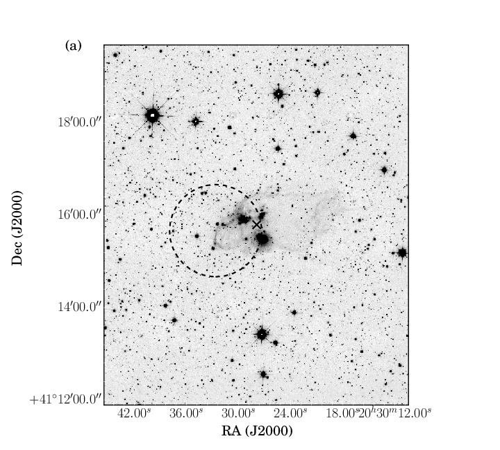
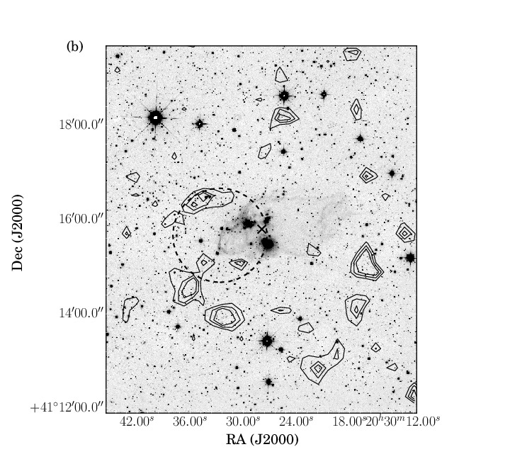
Figure 1: Stellar surface density contours using UKIDSS K-band data overlaid on the K-band UKIDSS image of the region associated with IRAS 20286+4105 - (a) results obtained using the star count method where no contours are seen above the mode+2$\sigma$ level (b) results obtained with NN algorithm. Contour levels are from mode+2$\sigma$ in steps of 1$\sigma$. The $\times$ sign represents the position of the IRAS point source. The circle shows the expected position and extent of the cluster as estimated by Kumar, Keto & Clerkin (2006).

A sparsely populated cluster with 7 ‘true’ cluster members has been shown to be associated with IRAS 20286+4105 (Kumar, Keto & Clerkin, 2006). These authors have used the 2MASS K-band data and the star count method to detect this cluster. With the availability of higher sensitivity and better resolution UKIDSS data, we aim at studying the cluster in detail. As mentioned in Section 2.3.2, we use the K-band photometric data from the pipeline processed UKIDSS 8PLUS GPS catalog. The first step towards this is to identify the cluster before proceeding to study the physical properties of the stellar population associated with it. We choose the K-band which gives the advantage of sampling the more embedded members of the cluster. We select an area within 300″radius centered on the position of the IRAS point source.

Initially, we adopt the star count method outlined in Schmeja (2011). The entire field is subdivided into rectilinear grids of overlapping squares. For maintaining Nyquist special sampling interval, the separation between the squares is made to be half the length of the squares (Lada & Lada, 1995). This method then involves determining the number of stars in each individual square grid. Each square grid acts as a single point for producing the surface density map. The square grids with star counts greater than some significant threshold ($\sim$ 2 - 5$\sigma$) above the background are regions of density enhancements and hence are considered as potential cluster locations (Schmeja, 2011). In our case, the mode (0.019 stars $\rm arcsec^{-2}$ or 312 stars $\rm pc^{-2}$) of the grids is considered to be the background and the noise/fluctuation in them defines $\sigma$ which is estimated to be 0.005 stars $\rm arcsec^{-2}$ or 82 stars $\rm pc^{-2}$. We assume mode+2$\sigma$ as the threshold for identifying density enhancement centers. Deciding the grid size is a crucial factor. We vary the grid size from 60$\arcsec$ to 110$\arcsec$ and find 80$\arcsec$ to be optimal. This is also the value adopted by Kumar, Keto & Clerkin (2006). Figure 1 shows the K-band image and the stellar density contours above the mode+2$\sigma$ threshold. As is clearly evident from the figure, there are no stellar density contours above the mode+2$\sigma$ level associated with the IRAS source. In fact, the entire field does not show any density enhancement above the defined threshold. The dotted circle roughly shows the position and extent of the cluster as estimated by Kumar, Keto & Clerkin (2006).

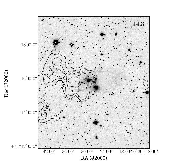
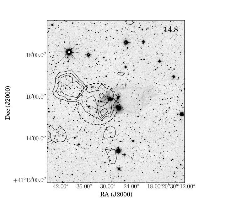
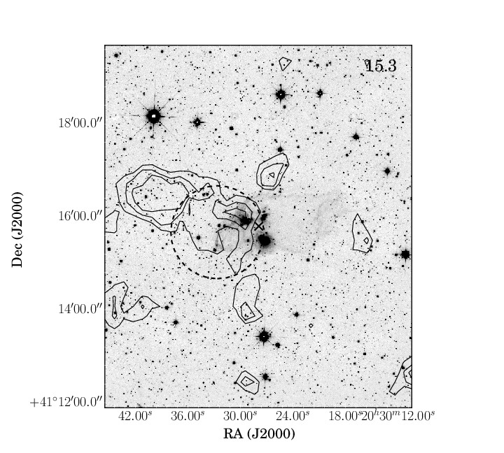
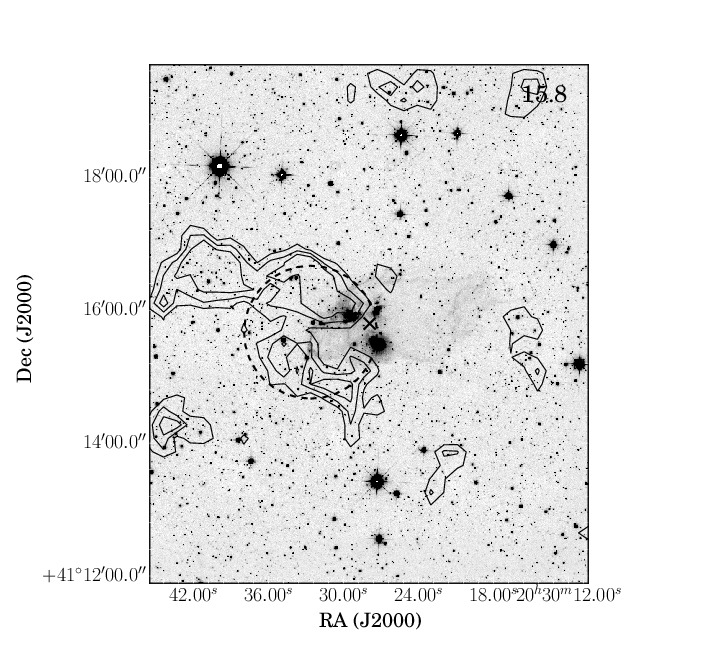
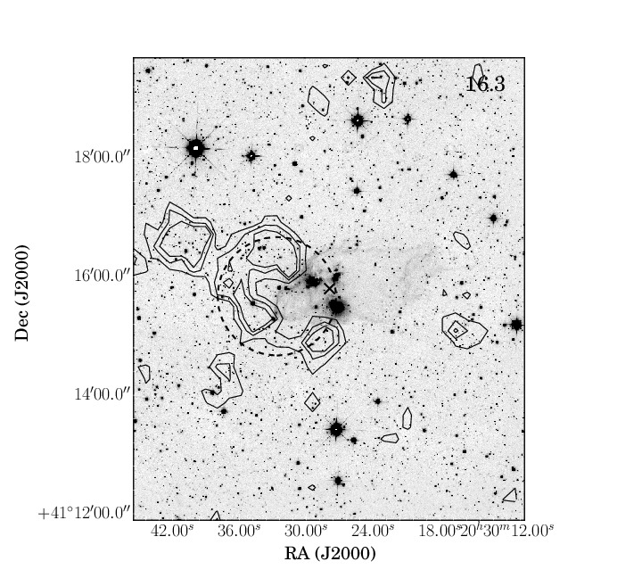
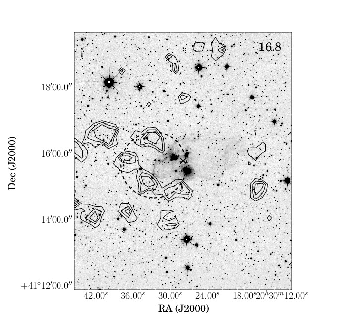
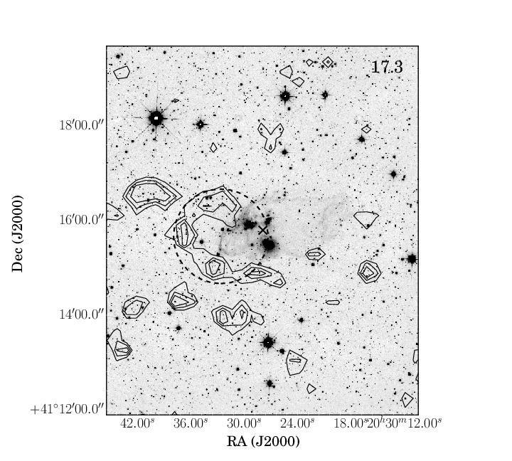
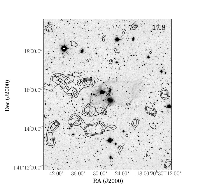
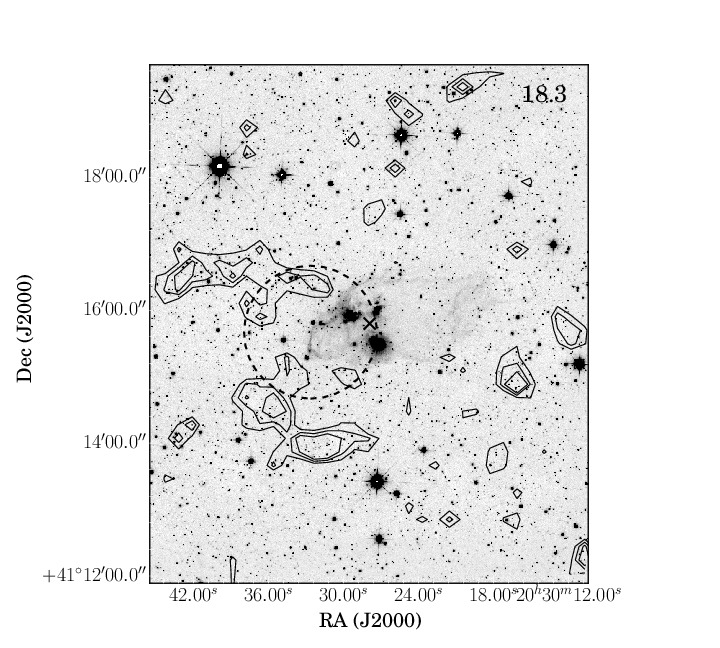
Figure 2: Stellar surface density contours using the NN algorithm using UKDISS data for different magnitude limits. The magnitude limit starts from the 2MASS limit of 14.3 mag and is increased in steps of 0.5 mag till the UKIDSS limit of 18.1 mag is reached. Contour levels are from mode+2$\sigma$ in steps of 1$\sigma$ overlaid on the UKIDSS K-band image. The $\times$ sign represents the position of the IRAS point source. The field of view of the images is same as in Figure 1. The circle shows the expected position and extent of the cluster as estimated by Kumar, Keto & Clerkin (2006).

In order to confirm the non-detection of the cluster, we use another cluster identification technique namely the nearest neighbour (NN) algorithm on the same dataset. Following the procedure outlined in Schmeja (2011) and Casertano & Hut (1985), the $j^{\rm th}$ nearest neighbour density is defined as

$$\rho_{j}=\dfrac{j-1}{S(r_{j})}$$ (1)

where $r_{j}$ is the distance of a star to its $j^{\rm th}$ nearest neighbor, $S(r_{j})$ is the surface area within $r_{j}$. NN density method depends only on the value of $j$. As given in Schmeja, Kumar & Ferreira (2008), $j$ = 20 is an optimum choice to detect clusters with 10 to 1500 members. We experimented on a range of values for $j$ and also found $j$ = 20 to be optimal. Low values of $j$ are sensitive to very small scale statistical fluctuations and higher values miss out the real small scale enhancements. The mode of the density values (0.026 stars $\rm arcsec^{-2}$ or 427 stars $\rm pc^{-2}$) gives the background and the fluctuation, $\sigma$ (0.004 per $\rm arcsec^{-2}$ or 66 stars $\rm pc^{-2}$) is the noise level. The results remain the same with this method as well and shown in Figure 1. We do not see any stellar density enhancement at the expected location of the previously detected cluster. However, few small-scale clusterings are seen to be present towards the periphery of the expected location of the cluster. Similar small-scale features are also seen elsewhere in the field.

In this paper we have used higher sensitivity and better resolution UKIDSS data in comparison to the 2MASS data used by Kumar, Keto & Clerkin (2006). The UKIDSS has a 5$\sigma$ limiting magnitude of 18.1 mag in the K-band (Dye et al., 2006; Lawrence et al., 2007), whereas the K-band magnitude limit (10$\sigma$) of 2MASS is 14.3 mag (Skrutskie et al., 2006). This prompted us to study the effect of sensitivity on cluster detection using the conventional techniques. This is achieved by repeating the above exercise with magnitude cuts starting from the 2MASS limit of 14.3 mag and proceeding in steps of 0.5 mag till we reach the 5$\sigma$ UKIDSS limit. Figure 2 shows the result at each magnitude limit. As seen in the figure, the stellar density enhancement is clearly evident at the 2MASS limit of 14.3 mag and is fairly consistent with the result obtained by Kumar, Keto & Clerkin (2006) (see their Fig. 1). In comparison to the results obtained by Kumar, Keto & Clerkin (2006), the cluster seems to be extended in the north-east direction. The signature of the cluster is clearly visible upto the magnitude cut-off of 16.3 mag. However, beyond this limit, the surface density contours appear to be fragmented into small scale enhancements mostly towards the eastern side of the expected location of the cluster.

This probably can be understood from the following consideration. As the magnitude limit is increased, the data set probes fainter sources which implies increase in source density. This increase includes both genuine cluster members as well as background contamination in the line of sight. In this case, the background increases by more than a factor of 10 from $\sim$ 25 stars $\rm pc^{-2}$ at 14.3 mag cut to $\sim$ 330 stars $\rm pc^{-2}$ at 18.3 mag which is close to the 5$\sigma$ UKIDSS limit. Given the fact that the cluster associated with IRAS 20286+4105 is a sparsely populated one, it is likely that the overwhelming background suppresses the cluster stellar density enhancement as we proceed towards fainter limits. The small scale features can be taken to be mostly due to fluctuations in the background. Another reason for these small-scale fluctuations could be the apparent over density of sources towards the east of the IRAS 20286+4105 cloud which is shown in later sections to harbour two dense clumps with low stellar content. Given the non-detection of the cluster using the new UKIDSS data, we could not proceed further towards a detailed study. In order to gain a better insight into the results obtained, in a forthcoming work (in preparation), we aim at using UKIDSS data for investigating this effect of sensitivity on cluster detection for a large sample of clusters already detected with 2MASS data.

3.2 Stellar population around IRAS 20286+4105

3.2.1 Identification of YSOs

IRAS 20286+4105 is a star forming complex in which previous studies have indicated the presence of young stellar objects (YSOs) (Varricatt et al., 2010). In this section we study the nature of the stellar population around IRAS 20286+4105 and identify candidate YSOs in this region. We use IRAC photometric data for this study. MIR colours are efficient tools to identify young stars, especially to distinguish between stars with disks and envelopes (Allen et al., 2004; Megeath et al., 2004; Simon et al., 2007; Gutermuth et al., 2008). In comparison with the NIR (e.g. JHK bands) emission from young stars, the MIR IRAC bands sample a significant fraction of emission from circumstellar material over the stellar photosphere. The IRAC images of the region associated with IRAS 20286+4105 display an elliptical shaped cloud. To ensure that we include the entire cloud and also a significant portion of the surrounding region, we consider a region of radius 150$\arcsec$ centered on the position of the IRAS point source. We detect 100 sources within this region that have good quality data in all four IRAC bands (3.6, 4.5, 5.8 and 8 $\rm\mu m$). We adopt the following four schemes to identify candidate YSOs. It is worth mentioning here that we are considering only those sources detected in all four IRAC bands hence probing only a sub-sample of YSOs.

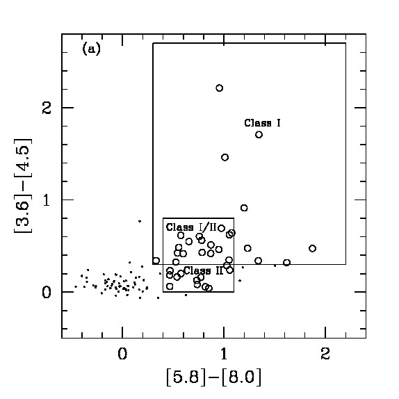
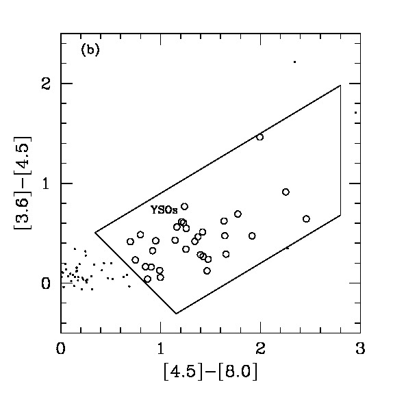
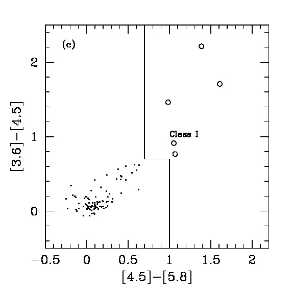
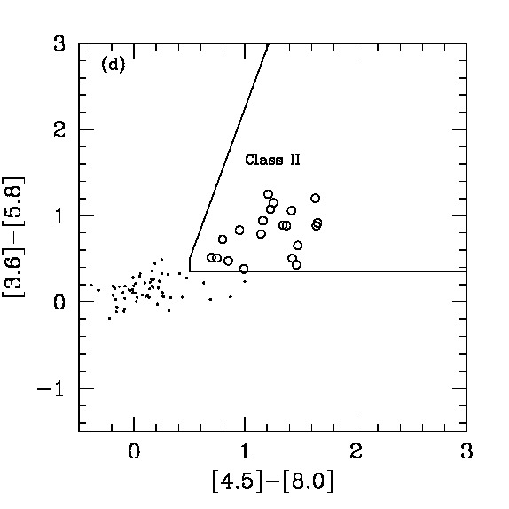
Figure 3: Colour-colour diagrams for the schemes discussed. (a) Allen et al. (2004) (b) Simon et al. (2007) (c) Gutermuth et al. (2008) Class I and (d) Gutermuth et al. (2008) Class II. The open circles represent the identified YSOs.

1. Lada (1987) define the IRAC spectral index to be

   $$\alpha_{\rm IRAC}=\dfrac{{\rm log}(\lambda F_{\lambda})}{{\rm log}(\lambda)}$$ (2)

   which is then used to classify YSOs. Using linear regression to the observed IRAC fluxes, we estimate the spectral index and classify the sources based on the criteria outlined in Chavarría et al. (2008). Class I sources ($\alpha>$ 0) are embedded sources with circumstellar disks and envelopes; Class II, or classical T Tauri stars (-2 $<\alpha<$ 0) have significant circumstellar disks, strong emission lines and substantial IR or UV excesses; Class III, or weak emission T Tauri stars ($\alpha<$ -2) have weak or no emission lines and negligible excesses. Following the above criteria, we identify 10 Class I and 37 Class II sources.

2. IRAC [3.6] – [4.5] vs [5.8] – [8.0] color-color (CC) diagram is also useful for classifying proto-stellar objects into their various evolutionary stages, such as Class I, Class II and Class III (Allen et al., 2004). Class I and Class II sources are identified based on their location in the CC plot. We identify 9 Class I, 16 Class I/II and 12 Class II candidate YSOs using boxes to demarcate the regions occupied by Class I and Class II sources as discussed in Vig et al. (2007).

3. The third scheme is based on the method proposed by Simon et al. (2007). They use the [3.6] – [4.5] and [4.5] – [8.0] colours to identify likely YSOs. Their set of colour criteria, which include the removal of galaxies and sources with contamination from polycyclic aromatic hydrocarbon emission, do not differentiate between Class I and II sources. Following this we identify 32 YSOs in our region.

4. Gutermuth et al. (2008) also use [3.6] – [4.5] vs [4.5] – [5.8] CC diagram for identifying protostellar candidate (Class I) sources and [3.6] – [5.8] vs [4.5] – [8.0] for pre-main sequence stars with circumstellar disk (Class II). The criteria proposed by them also filters out extra-galactic contaminants from the source list. We identify 5 Class I and 20 Class II candidate YSOs.

The CC diagrams for the various identification schemes are shown in Figure 3. Using the IRAC colors and based on the above four schemes, we identify a total of 78 YSOs within 150$\arcsec$ of IRAS 20286+4105. Figure 4 shows the distribution of the identified YSOs, which are highlighted on the 3.6 $\rm\mu m$ IRAC image. The figure also shows the 1280 MHz radio contours (see Section 3.3). As seen in the figure, YSOs are predominantly distributed towards the east beyond the arc-like ionized emission. A possible picture of triggered star formation is explored in Section 3.3. All the YSOs located inside the IRAS 20286+4105 cloud are found to be Class I sources which appear to cluster near the center of the cloud close to the position of the IRAS point source. These sources are classified as Class I YSOs in atleast one of the four schemes. Other parts of the cloud do not seem to harbour any YSOs. The Class I YSOs located inside the cloud are numbered from 1 to 6 and listed in Table 2. Sources 1, 2, 3, and 4 are the sources A, B, C, and D of Varricatt et al. (2010). These sources are discussed by them to be surrounded by nebulosities and showing reddening and/or IR excess. It should be noted here that sources 1 and 4 do not have available IRAC catalog magnitudes in the 5.8 and 8.0 $\rm\mu m$ bands. The magnitudes used here are estimated using the IRAF task ‘qphot’.

The MIPS 24 $\rm\mu m$ image shows the presence of two nearly spherical, bright regions with the northern one (which is saturated in the core) being extended to the east (see Section 3.5 and figure therein). Sources 1 and 2 are associated with the northern region and source 4 is associated with the southern region. The eastern extension of the northern region includes sources 3 and 5. No 24 $\rm\mu m$ emission is seen towards source 6.

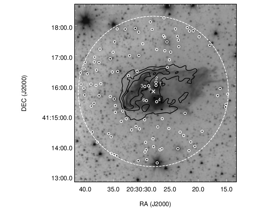
Figure 4: The distribution of YSOs (white open circles) are marked on Spitzer 3.6 $\rm\mu m$ band image. Overlaid on the image are the 1280 MHz contours (generated using the convolved low resolution map, see Section 3.3). The contour levels are at 5, 10 and 15 times the $\sigma$ (0.187 mJy/beam) level. The large dashed white circle shows the 150″radius region, centered on the IRAS point source position, used for studying the YSO population. The $\times$ mark denotes the position of the IRAS point source.

3.2.2 Spectral energy distribution of selected YSOs

In order to determine the stellar parameters of the six YSOs (Sources 1 to 6) located inside the cloud, we model the spectral energy distributions (SEDs) using the command-line version of the SED fitting tool of Robitaille et al. (2007) which uses YSO models from Robitaille et al. (2006). The YSO models are computed by adopting Monte Carlo based radiative transfer algorithms which use various combinations of central star, disk, infalling envelope, cavities carved out by bipolar outflows. A reasonably large parameter space is explored in these models.

We use NIR, MIR and FIR data from 2MASS, UKIDSS (for source 5), Spitzer-IRAC, Spitzer-MIPS, WISE(22 $\rm\mu m$), and Herschel. Sources 1, 4, and 6 have WISE point source counterparts. Source 2 lies at an angular distance of 6″ from source 1. We use the WISE 22 $\rm\mu m$ point source magnitudes as upper limits given the poor resolution of the images. From the radial profiles of isolated point sources in the 22 $\rm\mu m$ image, we estimate the FWHM to be $\sim 18\arcsec$. For sources 1 and 2 we use the same upper limit as the separation between them is less than the resolution of the image. Spitzer-MIPS 24 $\rm\mu m$ point source magnitude for source 3 is also taken as an upper limit given the contamination from source 5. For source 5, the 24 $\rm\mu m$ upper limit is estimated by extracting the flux within an appropriate aperture centered on the source. For all the sources, flux densities are also estimated from the Herschel maps and used as upper limits in the SED fitting. We have included a conservative 10% error on the fluxes while fitting the SED models. Distance and visual extinction are taken as free parameters in the models. We adopt a distance range from 1.4 - 1.8 kpc. We estimate the extinction by de-reddening the stars using the JHK colour-colour plot (Kumar, Ojha & Davis, 2003; Ojha et al., 2004). This is done by shifting them along the reddening vector to a line drawn tangential to the turn-off point of the main sequence locus (Tej et al., 2006). The estimated values range from A${}_{v}=0$ to 20 mag and this range is used for the model fitting.

The SED fitting tool gives the best fit model as well as a set of well fit models ranked by their $\chi^{2}$ values. We considered only those models which satisfy

$\chi^{2}-\chi^{2}_{\rm best}<3$ (per data point)

The resulting SEDs are shown in Figure 5. The weighted (inverse $\chi^{2}$ of each model is taken as the weight) mean and standard deviations of the parameters obtained for these models are listed in Table 2. From the model fitted parameters, majority of the Class I YSOs located inside the cloud are found to be intermediate mass stars with the derived masses ranging between $\rm 2.5~{}M_{\odot}$ to $\rm 5.0~{}M_{\odot}$. Source 5 fits to a low-mass star of mass $\rm 1.7~{}M_{\odot}$. Given the models used and the large parameter space explored with few data points, the derived values of the various parameters should be treated as indicative only.

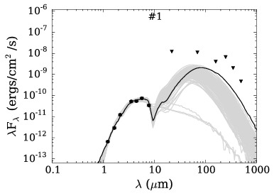
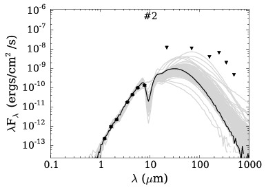
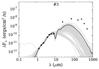
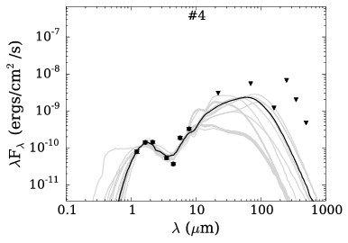
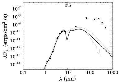
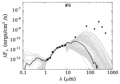
Figure 5: SED fitting of the six Class I YSOs using the command-line version of the SED fitting tool of Robitaille et al. (2007). The filled circles show the input fluxes and filled triangles are the upper limits, black line shows the best fit and gray lines show the subsequent good fits for $\chi^{2}-\chi^{2}_{\rm best}<3$.

Table 2: Stellar parameters obtained for the six sources located inside the cloud. The values are the weighted mean and standard deviations of the model output parameters obtained using the command-line version of the SED fitting tool of Robitaille et al. (2007). The values retrieved from the best fitting model is given in parenthesis.

$\#$	RA	DEC	log t∗	M∗	log Mdisk	log $\dot{M}_{\rm disk}$	log T∗	log LTotal	Av
	(J2000)	(J2000)	(yr)	(M⊙)	(M⊙)	(M⊙/yr)	(K)	$({\rm L}_{\odot})$	(mag)
1	20:30:27.4	41:15:59.8	4.92 $\pm$ 0.77	4.69 $\pm$ 1.52	-1.64 $\pm$ 0.79	-6.92 $\pm$ 1.13	3.71 $\pm$ 0.14	2.21 $\pm$ 0.27	11.35 $\pm$ 4.96
			(4.63)	(6.02)	(-2.01)	(-8.32)	(3.65)	(2.33)	(6.27)
2	20:30:27.4	41:16:06.0	3.84 $\pm$ 0.72	3.06 $\pm$ 1.83	-1.64 $\pm$ 0.74	-5.84 $\pm$ 1.19	3.64 $\pm$ 0.13	2.16 $\pm$ 0.33	10.01 $\pm$ 4.11
			(3.49)	(2.80)	(-2.31)	(-6.35)	(3.62)	(2.14)	(4.12)
3	20:30:29.4	41:15:57.6	4.61 $\pm$ 1.32	3.56 $\pm$ 1.68	-1.93 $\pm$ 1.06	-6.72 $\pm$ 1.59	3.77 $\pm$ 0.26	2.19 $\pm$ 0.34	7.73 $\pm$ 4.91
			(3.65)	(2.74)	(-1.53)	(-6.21)	(3.62)	(2.11)	(0.85)
4	20:30:27.3	41:15:27.3	5.20 $\pm$ 0.60	4.98 $\pm$ 0.97	-1.98 $\pm$ 1.03	-6.61 $\pm$ 1.03	3.77 $\pm$ 0.10	2.36 $\pm$ 0.19	6.52 $\pm$ 3.17
			(4.66)	(3.73)	(-1.38)	(-5.03)	(3.64)	(2.19)	(6.22)
5	20:30:28.7	41:15:59.1	3.89 $\pm$ 1.41	1.69 $\pm$ 2.28	-2.02 $\pm$ 0.39	-5.65 $\pm$ 1.78	3.70 $\pm$ 0.30	1.87 $\pm$ 0.58	11.56 $\pm$ 3.27
			(3.42)	(0.44)	(-1.74)	(-4.83)	(3.56)	(1.53)	(9.67)
6	20:30:29.1	41:15:29.6	5.66 $\pm$ 1.31	2.49 $\pm$ 1.29	-2.45 $\pm$ 0.90	-7.66 $\pm$ 1.38	3.88 $\pm$ 0.23	1.69 $\pm$ 0.41	9.04 $\pm$ 6.34
			(6.77)	(4.67)	(-2.85)	(-8.9)	(4.18)	(2.49)	(1.63)

3.3 Emission from ionized gas

The radio continuum maps probing the ionized gas associated with IRAS 20286+4105 at 610 MHz, 1280 MHz and 4.89 GHz are shown in Figure 6 and the details of the maps are given in Table LABEL:radiotab.

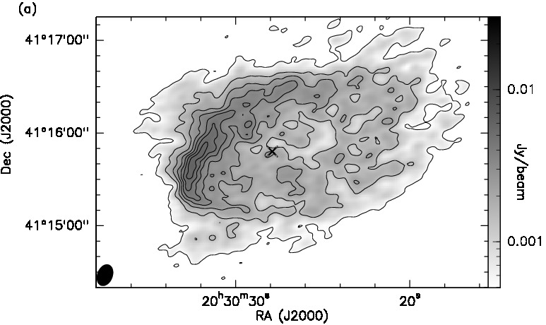
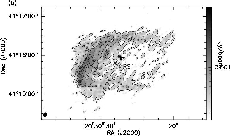
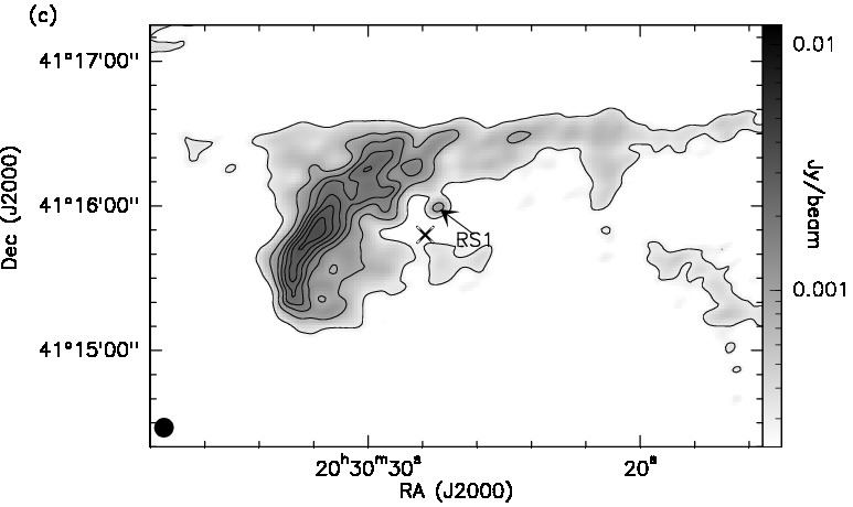
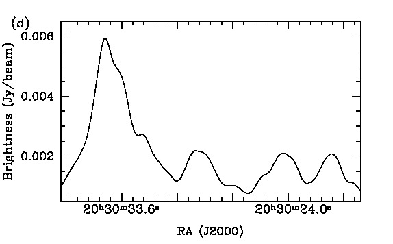
Figure 6: Radio continuum maps at (a) 610 MHz (b) 1280 MHz and (c) 4.89 GHz for the region around IRAS 20286+4105. The contour levels are at 3, 8, 13, and 18 $\sigma$ levels, where $\sigma$ is the rms noise in the maps. For the 610 MHz map 23, 28, and 33 $\sigma$ levels are also shown. The IRAS source position is marked with a $\times$ symbol. The intensity profile along 90^∘ PA (taken east of north) at $\delta$ = $\rm 41^{\circ}15\arcmin 48\arcsec$ of radio emission at 610 MHz is shown in (d).

Table 3: Details of the radio continuum maps from GMRT and VLA. The integrated flux values are upto the 3$\sigma$ level, where $\sigma$ is the rms noise in the maps.

Details	610 MHz	1280 MHz	4.89 GHz
Date of Observation	09 April 2004	28 September 2002	15 April 1988
Synth. beam	7$\arcsec$.26 $\times$ 5″.04	2″.91 $\times$ 2″.26	4″.07 $\times$ 4″.01
Integrated Flux (mJy)	781	508	150
rms noise (mJy/beam)	0.170	0.070	0.100

The radio maps clearly show a bright arc-like emission toward the east and extending northwards with a decreasing intensity distribution in the south-west direction. The GMRT maps show the presence of diffuse emission in the entire cloud. The diffuse emission is more extended at 610 MHz compared to the 1280 MHz map. The 4.89 GHz VLA map mostly shows the bright arc. The intensity variation of the ionized region along a central declination is also shown in Figure 6 (d). The profile resembles the characteristic intensity distribution of a cometary HII region as described in Wood & Churchwell (1989). We discuss the cometary nature of the radio morphology in detail toward the end of this section.

Apart from the diffuse emission, the 1280 MHz map peak coincides with a point-like compact knot (hereafter RS1) located at $\alpha_{2000}$=$\rm 20^{h}30^{m}27.34^{s}$; $\delta_{2000}$=$+41^{\circ}$15′58.51″. This knot is also clearly seen in the 4.89 GHz map. The position of this knot is toward the centre of the cloud and west of the bright, diffuse arc-type emission. Indication of this radio knot can also be seen in the map presented by McCutcheon et al. (1991) (see their Fig. 1). However in the 610 MHz map, RS1 is not as prominent given the dominant diffuse emission at this frequency. A more detailed study of RS1 is presented in the next section.

The physical properties of the ionized gas in this region are derived from the flux density measurements obtained from the radio maps. The number of hydrogen ionizing photons (h$\nu$ $>$ 13.6 eV) per second required to maintain the ionization of the nebula and hence the spectral type of the ionizing star is estimated using the 1280 MHz flux density and the formulations discussed in Martín-Hernández, van der Hulst & Tielens (2003) and Panagia (1973). Assuming the emission to be optically thin at this frequency and a single ionizing source responsible for the same, the number of Lyman continuum photons is estimated using the following expression from Martín-Hernández, van der Hulst & Tielens (2003),

$$N_{\rm lyc}=4.634\times 10^{46}\left(\dfrac{T_{e}}{10^{4}{\rm K}}\right)^{-0.45}\left(\dfrac{\nu}{{\rm 5~{}GHz}}\right)^{0.1}\left(\dfrac{D}{{\rm 1~{}kpc}}\right)^{2}$$ (3)

$$\times\left(\dfrac{S_{\nu}}{{\rm 1~{}Jy}}\right)a_{\nu}^{-1}[{\rm s^{-1}}]$$

where, $T_{e}$ is the electron temperature, $\nu$ is the frequency in GHz, $S_{\nu}$ is the integrated flux, $D$ is the heliocentric distance and $a_{\nu}$ is the correction factor (taken as unity similar to Martín-Hernández, van der Hulst & Tielens (2003)). $T_{e}$ is estimated to be $\sim$ 7300 K using the following equation from Deharveng et al. (2000)

$$T_{e}[K]=(372\pm 38)D_{G}+4260\pm 350$$ (4)

where $D_{G}$ is the Galactocentric distance of the source which is determined to be 8.16 kpc following the expression from Xue et al. (2008). We estimate log₁₀($N_{\rm lyc}$) to be 46.79 which translates to a main-sequence spectral type between B0.5 – B0 (see Table 2 of Panagia (1973)). The spectral type determined from this work is within one subclass of the estimates obtained from previous radio continuum studies by Odenwald & Schwartz (1989) and McCutcheon et al. (1991) after scaling to the distance and electron temperature used in our study. Verma et al. (2003) carried out the radiative transfer modeling of two FIR cores located towards the cloud centre (see Section 3.5) using MIR and FIR data and estimated the spectral type of the sources associated with these cores to be between B0.5 - B0. Their modeling predicted no radio emission. It should be noted here that the GMRT maps do not show any radio peaks associated with the cores except the radio knot RS1 even though diffuse radio emission is detected in the entire cloud.

We estimate the emission measure and the electron density of the ionized region associated with IRAS 20286+4105 by assuming the radio emission to be free-free from an isothermal, spherically symmetric and homogeneous medium (Tej et al., 2006; Vig et al., 2014). For this, we convolve the 4.89 GHz and 1280 MHz maps to the resolution of 610 MHz map which has the lowest resolution ($7\arcsec.26\times 5\arcsec.04$). The extent of the eastern, bright radio arc is found to be roughly 15 - 20″ wide if we include only the bright emission region (above 15$\sigma$). The peaks of these convolved radio maps are located within this bright arc. The 1280 MHz map shows two discrete peaks (5.76 mJy/beam at $\alpha_{2000}$=$\rm 20^{h}30^{m}31.69^{s}$; $\delta_{2000}$=$\rm+41^{\circ}$15′51.51″and 5.47 mJy/beam at $\alpha_{2000}$=$20^{h}30^{m}32.43^{s}$; $\delta$=$\rm+41^{\circ}$15′38.20″) on the arc. The 4.89 GHz map shows a single peak which matches within $\sim 3\arcsec$ of the brighter 1280 MHz peak. The 610 MHz map does not clearly display any discrete peak and shows a rather elongated flux enhanced region. The location of the peak flux density lies within $\sim 1.5\arcsec$ of the secondary peak of 1280 MHz. From the 1280 MHz and 4.89 GHz peak fluxes, we derive the emission measure and the electron density to be $\rm 1.75\times 10^{5}\,cm^{-6}\,pc$ and $\rm 1.9\times 10^{3}\,cm^{-3}$, respectively, for the estimated electron temperature of 7300 K.

The ionized emission is also probed in the optical and NIR using H$\alpha$ (656.8 nm) and Br$\gamma$ (2.166 $\rm\mu m$) emission lines. Figure 7 shows the continuum-subtracted H$\alpha$ and Br$\gamma$ images. The signal-to-noise ratio in the continuum-subtracted Br$\gamma$ image is rather poor. Nevertheless, we clearly detect a faint arc of emission. The H$\alpha$ image shows a much more extended arc, whereas the Br$\gamma$ emission is prominent mostly towards the southern part of the arc. However, in the absence of flux calibrated images, it is difficult to decouple the effect of instrument sensitivities. We have overlaid 1280 MHz radio contours (generated using the convolved low resolution map) on the H$\alpha$ line emission image. This shows the correlation between the ionized components at optical, infrared and radio wavelengths. The optical and NIR continuum-subtracted line images trace the arc-like radio morphology. However, since the radio emission is least affected by extinction, the maps detect the extended, faint, and diffuse emission spread over the entire cloud associated with IRAS 20286+4105.

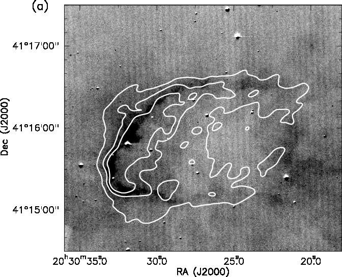
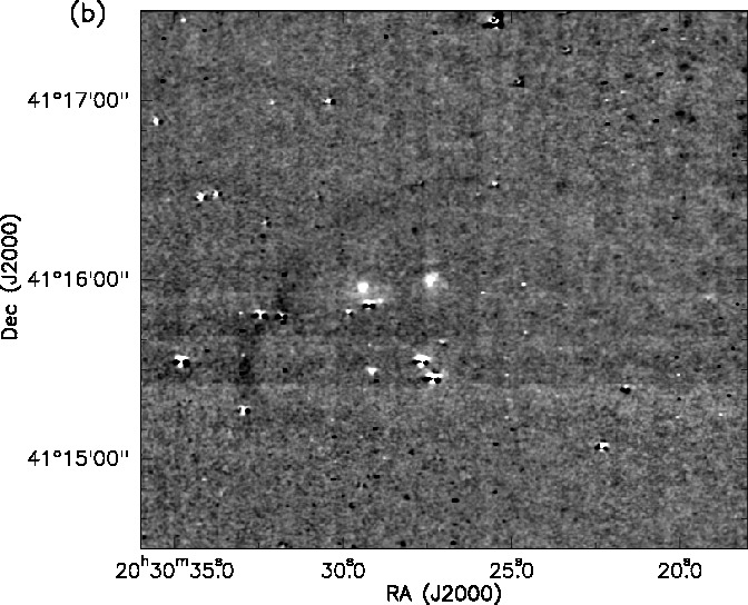
Figure 7: Ionized emission in the (a) H_α and (b) Br$\gamma$ for the region associated with IRAS 20286+4105. Overlaid on the H_α image are the 1280 MHz contours (generated using the convolved low resolution map). The contour levels are at 5, 10 and 15 times the $\sigma$ (0.187 mJy/beam) level. Residuals of continuum subtraction are seen in the images.

A 2MASS source (J20303183+4114548: J = 11.845 mag; H = 11.587 mag; K_s = 11.458 mag) with an optical counterpart (SDSS r magnitude = 14.445 ) lies within 4″ of the brighter 1280 MHz peak. The second radio peak is also seen to be within 4″ of another 2MASS source (J20303274+411540 - J = 15.795; H = 14.849; K_s = 14.568) with an optical counterpart (SDSS r magnitude = 19.9 mag). The NIR magnitudes and colours of both these sources, which lie within the radio arc, suggest that these are likely to be main-sequence field sources in the line of sight. Apart from these, the nearest identified IRAC YSO is located $\sim 9\arcsec$ towards the east of the radio peaks and hence unlikely to be associated with them.

The observed radio arc points towards the direction of the Cygnus OB2 cluster. IRAS 20286+4105 cloud falls within the radius of influence of this cluster (Schneider et al., 2006; Roy et al., 2011) being located at a distance of $\sim$20 pc from the cluster centre. Based on the age of the Cyg OB2 cluster and the distance to it, it is possible that the ionization front emanating from the massive stellar population of the cluster would have reached and ionized the IRAS 20286+4105 cloud. From the mass, luminosity and the geometry of the IRAS 20286+4105 cloud, Roy et al. (2011) suggest that the radio emission is possibly due to this external ionization field. It should be noted here that the authors do not give any quantitative proof for the above inference.

However, given the cometary morphology of the HII region associated with IRAS 20286+4105 and the presence of a nearby supernova remnant, SNR G079.8+01.2 (IRAS 20281+4106) (Setia Gunawan et al., 2003), we attempt to explore a different angle where a likely association of both is invoked. In Figure 8, we show the relative location of SNR G079.8+01.2 and the IRAS 20286+4105 cloud in the plane of the sky. SNR G079.8+01.2 lies in the region belonging to the Cygnus OB2 association at an angular distance of $\sim 6.5\arcmin$ from the position of the radio peak of IRAS 20286+4105 cloud. Based on the IRAS flux densities, Parthasarathy, Jain & Bhatt (1992) have identified IRAS 20281+4106, associated with the SNR, as a possible Class I YSO. These authors have assumed IRAS 20281+4106 to belong to the Cygnus OB2 association ($\rm d=1.7~{}kpc$). Using the $\rm HCO^{+}$ line velocity measurements given in Shirley et al. (2013) and the rotation curve of Brand & Blitz (1993), we estimate the kinematic distances to IRAS 20286+4105 and SNR G079.8+01.2 to be 3.8 and 4.1 kpc, respectively. Based on these estimates, we assume the SNR to be at the same distance as the IRAS 20286+4105 cloud. However, we adopt the distance of 1.61 kpc for both the complexes.

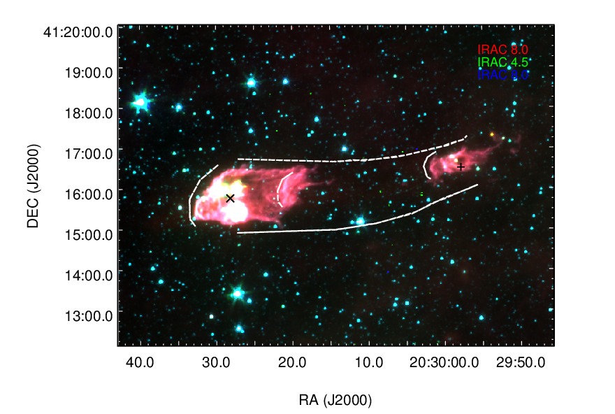
Figure 8: Spitzer IRAC 3 - color composite image of the region around IRAS 20286+4105. The position of IRAS source and SNR G079.8+01.2 are marked with ’x’ and ’+’, respectively. The figure also marks the curvatures and the northern and southern edges based on visual inspection.

Focusing on the morphology of the HII region, there are several models proposed in literature for the mechanisms behind such morphology that is commonly observed in HII regions. Reid & Ho (1985) were the first to propose the relative motion between the ionizing source and the extended molecular environment. This led to the ‘bow-shock’ model (van Buren et al., 1990; Mac Low et al., 1991; van Buren & Mac Low, 1992), which requires highly supersonic motion of a wind-blowing, ionizing star through dense surrounding material. The other frequently adopted model is the ‘champagne-flow’ model which assumes the ionizing star to be nearly stationary with respect to the molecular cloud. The cometary morphology in this case is attributed to the steep density gradient existing in the surrounding medium (Israel, 1978; Tenorio-Tagle, 1979). The column density map derived using Herschel data reveal the presence of a high-density clump in the middle of the IRAS 20286+4105 cloud (see Section 3.5). The ionized gas distribution shows a decrease in intensity in the south-west direction towards the clump which is opposite to what is expected from the ‘champagne-flow’ model and hence this model is unlikely to explain the observed cometary morphology.

The occurrence of a bow-shock in the IRAS 20286+4105 cloud requires a star with large velocity generally termed as a ‘runaway’ star. Two mechanisms are generally proposed to explain the origin of their high velocities. One of these is the binary supernova scenario where the ‘runaway’ star is initially part of a binary system. It acquires high velocities when its binary companion explodes as a supernova (Blaauw, 1961; Moffat et al., 1998). The other mechanism involves dynamical ejection from a dense cluster (Poveda, Ruiz & Allen, 1967; Gies & Bolton, 1986). Hoogerwerf, de Bruijne & de Zeeuw (2001) give evidences for both mechanisms based on accurate astrometry observations. Our aim is to first quantitatively attribute the bow-shock mechanism with the observed cometary morphology. Subsequently, we try to probe the likely connection between the SNR and the HII region.

A ‘bow-shock’ is detected at the stand-off distance ($\rm r_{s}$) from the ionizing star where the ram pressure and momentum flux of the wind and the interstellar medium (ISM) balance (van Buren et al., 1990; Mac Low et al., 1991). Equating these quantities, the stand-off distance is shown to be (van Buren & McCray, 1988),

$$r_{s}=1.78\times 10^{3}\sqrt{\frac{\dot{M}v_{\infty}}{\mu_{\rm H}n_{\rm H}v_{\rm\star-ISM}^{2}}}\ {\rm pc}$$ (5)

where, $\dot{M}$ is mass-loss rate from star in M${}_{\odot}\,\rm yr^{-1}$ and $v_{\infty}$ is the terminal velocity of the stellar wind in $\rm km~{}s^{-1}$. $\mu_{\rm H}$ and $n_{\rm H}$ are the mean mass per hydrogen nucleus and the hydrogen gas density in $\rm cm^{-3}$, respectively. $v_{\star-\rm ISM}$ is the velocity of star with respect to ISM in km $\rm s^{-1}$. The mass-loss rate and the terminal velocity are obtained using the following equations from Mac Low et al. (1991).

$$\dot{m}=2.0\times 10^{-7}\left({L}/{L_{\odot}}\right)^{1.25}\\$$ (6)

$${\rm log}\ v^{\prime}_{\infty}=-38.2+16.23\ {\rm log}\ T_{{\rm eff}}-1.70\ ({\rm log}\ T_{{\rm eff}})^{2}$$ (7)

where, $L$ is the stellar luminosity, $L_{\odot}$ is the solar luminosity and $T_{{\rm eff}}$ is the effective temperature of star. In Equation 5, $\dot{M}=\dot{m}\times 10^{-6}\,{\rm M}_{\odot}$ $\rm yr^{-1}$, $v_{\infty}=v^{\prime}_{\infty}\times 10^{3}\,\rm km\,s^{-1}$. The luminosity and effective temperature are $2\times 10^{4}-4.8\times 10^{4}L_{\odot}$ and 26200 - 30900 K, respectively for the estimated spectral type of B0.5 - B0 (Panagia, 1973). It is to be noted here that the recently released parallax catalog from URAT (Finch & Zacharias, 2016) has the astrometry of most 2MASS sources in the Cygnus region. However, in our case, we do not have any 2MASS counterpart of the radio peak which is the likely position of the ionizing star. Thus, we lack information regarding the astrometry of the ionizing star. Hence, for our calculations, we adopt a typical space velocity of $\rm\sim 10~{}km\,s^{-1}$ (van Buren & Mac Low, 1992) for the supersonically moving ionizing star. Plugging in these values in the above equations, we determine the mass-loss rate, $\dot{M}=2.2-6.3\times 10^{-8}\,{\rm M}_{\odot}$ $\rm yr^{-1}$ and the terminal velocity $v_{\infty}=2.1-2.5\times 10^{3}\,{\rm kms^{-1}}$.

The medium through which the star moves would be a combination of ionized and neutral medium. If we consider the HII region to be fully ionized, then the electron density, $n_{\rm e}=n_{\rm H}$. Taking $\rm\mu_{H}=0.61$ (for a fully ionized medium) and using Equation 5, we estimate the stand-off distance to lie between 0.05 - 0.09 pc which translates to 6.8″- 12.6″. However, if we consider a neutral medium, then we use $n_{\rm H}=1.2\times 10^{4}\,\rm cm^{-3}$ derived from the column density maps for Clump 1 (refer to Section 3.5) and $\mu_{\rm H}=1.4$. In this case, the stand-off distance lies between 0.01 - 0.03 pc or 1.8″- 3.4″. From the 1280 MHz radio map, the angular separation between the peak and the ‘edge’ of the bright emission is estimated to be $\sim$ 7″ . This is consistent with the stand-off distance calculated for the fully ionized case thus supporting the bow-shock scenario. A further point to note is regarding the H₂ line emission of the region associated with IRAS 20286+4105 which is presented in Varricatt et al. (2010). The H₂ line image also shows the presence of an arc, the location of which matches with the position of the radio arc seen in our maps. Morphologically, the H₂ line emission is seen to be irregular compared to the radio emission. Considering the above bow-shock scenario, it is likely that this H₂ line emission is shock-excited .

The morphology of the marked arcs and the shape of the northern and southern edges of the IRAS 20286+4105 cloud and the SNR, as highlighted in Figure 8, indicates their likely association. The curvature of the arcs points in the direction from the SNR to the cloud. Going by the binary supernova model, we expect the SNR to be the parent location of the star responsible for the bow-shock. For the assumed velocity of $\rm 10\,km\,s^{-1}$, we estimate the kinematic age (which is defined to be the time since this runaway star left its parent association) to be $\rm\sim 3\times 10^{5}yr$. The kinematic age thus derived can be considered as an upper limit since the initial velocity of the star could be higher compared to the velocity considered inside the cloud. The derived age is considerably shorter than the main-sequence lifetime of $\rm(12-16.4)\times 10^{6}yr$ (Mottram et al., 2011) of the ionizing star which is estimated to be of spectral type between B0 - B05. This difference in the ages is consistent with the fact that runaway stars acquire high velocities after an initial evolutionary phase as member of a close binary system in which the primary evolves for several million years before it explodes as a supernova and the runaway is ejected out of the system (Hoogerwerf, de Bruijne & de Zeeuw, 2001). The above analysis suggests that the radio emission seen in the IRAS 20286+4105 cloud is due to a possible runaway star which was likely associated with SNR G079.8+01.2 in the past.

The above picture has implication on the star formation activity in the IRAS 20286+4105 cloud as well. The SED model fitted ages of the six Class I YSOs located inside the cloud range between $\rm 7\times 10^{3}yr$ to $\rm 5\times 10^{5}yr$. If these are taken as representative values, then it is possible that this population is the result of a shock-triggered collapse of a pre-existing clump by an encroaching shock either from the strong stellar wind of the precursor of the supernova or originating from the energetics of the explosion itself. The collapse could also have been induced by the passing runaway star. Further evidence of triggered star formation is also seen towards the east beyond the radio arc where there is a over density of YSOs. The above interpretation finds strength in the morphology of IRAS 20286+4105 cloud and the SNR discussed earlier. However, it should be noted here that the simplistic calculations and the interpretations given above are based on model fitted age parameters and on the visual inspection of the projected morphology of the complex. With the given data, it is difficult to make further quantitative interpretation.

As is clear from previous discussions, two scenarios emerge related to the ionized emission associated with the IRAS 20286+4105 cloud. Without disqualifying the possibility of external ionization due to the massive stars of Cygnus OB2 cluster, we are inclined towards the bow-shock, ‘runaway’ star and the supernova picture. This is driven by the proximity of SNR G079.8+01.2 and the correlation seen in the morphology discussed and shown in Figure 8. Accurate distance estimates, identification of the ionizing star and determination of space velocity are required before we can conclusively ascertain the mechanism behind ionization in the cloud.

3.4 Nature of radio knot RS1

As mentioned in Section 3.3, a radio knot, RS1, is visible towards the center of the complex around 10″ north of the IRAS point source. RS1 is located at the peak position of the high resolution (2″.91 $\times$ 2″.26) 1280 MHz map and lies within $\sim$ 1.5″ of Source A and of 7″ of Source B of Varricatt et al. (2010). From narrow-band $\rm H_{2}$ observations, Varricatt et al. (2010) show the presence of two outflows associated with this region (see Fig. A40 of their paper). They suggest a deeply embedded source north of Source A to be responsible for the east-west aligned outflow and Source B to be the driving YSO for the other outflow. Based on the location, it is likely that RS1 is associated with the aligned outflow. Figure 9 shows the position of RS1 in comparison to the outflow directions given in Varricatt et al. (2010). As shown in the figure, there are a number of masers detected towards IRAS 20286+4105. The positions of H₂O & NH₃ masers detected by Urquhart et al. (2011) are coincident with that of RS1. Water masers are known for their closest association with outflows from young stars (de Buizer et al., 2005). It should be noted here that in some papers the IRAS point source position is listed against the detected masers which may not be the actual position of the masers.

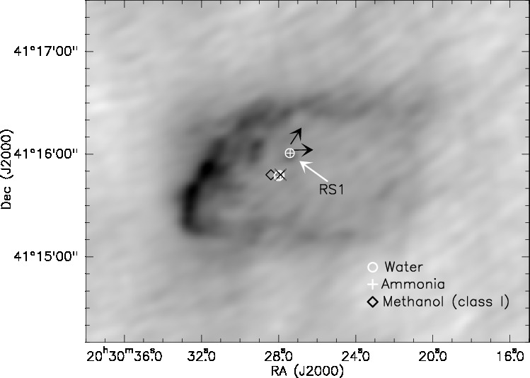
Figure 9: Position of RS1 and maser emission spots in the region are marked on the low resolution 1280 MHz radio image. Also marked as black arrows are the two possible collimated outflows discussed in Varricatt et al. (2010). The $\times$ shows the position of the IRAS point source.

To probe the radio nature of RS1, we investigate the radio SED obtained using the low resolution ($7\arcsec.26\times 5\arcsec.04$) maps. We integrate the flux within a square aperture of size 16″ covering RS1. Figure 10 shows the SED. The integrated flux obtained for RS1 from the 610 MHz map is considered as an upper limit since it includes significant contribution from the diffuse emission. The slope of this log-log plot is generally defined as the spectral index denoted by $\alpha$ (assuming $S_{\nu}\propto\nu^{\alpha}$). A spectral index of $\sim-0.5\pm 0.05$ is obtained using the flux densities at 1280 MHz and 4.89 GHz. The fitted slope is shown as a dotted line in the figure. The derived negative spectral index is not consistent with the value of $\sim-0.1$ expected from optically thin free-free emission. Rodriguez et al. (1993) show that when only free-free emission and absorption mechanisms are involved, the spectral index is always $\geqslant-0.1$ irrespective of the electron density and temperature distribution. Spectral indices below $-0.1$ are interpreted as co-existing synchrotron emission components with free-free emission. Such negative spectral indices are seen in Herbig-Haro objects which are associated with jets / outflows (Marti, Rodriguez & Reipurth, 1993). The above discussion indicates that RS1 is possibly associated with the shocked non-thermal emission from the detected outflow. Crusius-Wätzel (1993) explained that non-thermal emission associated with jets and outflows are due to the diffusive shock acceleration at working surfaces of jets, which moves into the ambient molecular cloud and boosts up the non-thermal emission over thermal free-free emission. For this mechanism to happen, a high density environment with strong magnetic field is required. Non-thermal emission due to stellar winds and associated jets are also discussed by Reid et al. (1995) who also show the correlation of water masers with non-thermal sources.

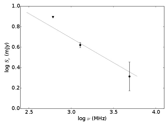
Figure 10: The radio SED of RS1. The dotted line shows the fitted spectral index slope using flux densities at 1280 MHz and 4.89 GHz. The upper limit to the flux density at 610 MHz is shown as a triangle.

In the infrared, RS1, which coincides with Source A of Varricatt et al. (2010), is an extreme red and embedded object with NIR colors of J - K = 6.4 and H - K= 2.63. These colors suggest large NIR excess that possibly indicates a highly extincted protostellar candidate (compare with Figure 7 of Tej et al. (2006)). The MIR IRAC colors place it in the location of Class I objects (YSO # 1) in the CC diagrams, consistent with the JHK colors. The SED modelling presented in Section 3.2 suggests an intermediate-mass star with an estimated mass of $~{}\rm 4.7\,M_{\odot}$ and a disk accretion rate of 1.2$\times 10^{-7}$ M_⊙/yr.

3.5 Emission from cold dust

The distribution of dust emission in the region around IRAS 20286+4105 is shown as a colour-composite image in Figure 11. The expanded view shows the complex under study. The image shows the presence of two bright nearly spherical regions with the northern one being extended towards the east. The cold dust environment sampled by 250 $\rm\mu m$ (red) emission is more extended and dominant towards the northern edge, whereas the warm dust sampled by the 24 $\rm\mu m$ (blue) emission is mostly localized in these two regions being brighter towards the southern one. These regions are also identified as the northern and southern cores and studied by Verma et al. (2003). From the radiative transfer modeling of the MIR and FIR data, these authors suggest the luminosities of the two cores to be consistent with ZAMS stars of spectral type B0.5 (northern core) and B0 - B0.5 (southern core).

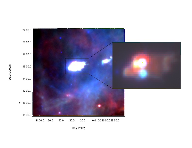
Figure 11: Three color composite image of the region around IRAS 20286+4105 with Herschel-SPIRE 250 $\rm\mu m$ (red), Herschel-PACS 70 $\rm\mu m$ (green) and 24 $\rm\mu m$ Spitzer-MIPS (blue) images.

The thermal dust emission peaks in the FIR and the Rayleigh-Jeans regime of the cold dust SED is covered by the Herschel bands (160 - 500 $\rm\mu m$). In this section we carry out detailed study of the physical properties of the cold dust environment associated with IRAS 20286+4105 using Herschel data.

3.5.1 Temperature and column density distribution

Following the procedure outlined in Battersby et al. (2011), Nielbock et al. (2012), Launhardt et al. (2013), and Mallick et al. (2015), a pixel-by-pixel modeling of this dust emission with a gray body/modified blackbody is adopted in order to generate temperature and column density maps of the region of our interest. For the preliminary steps, the Herschel data compatible software HIPE is used. The image units of PACS ($\rm Jy\,pixel^{-1}$) and SPIRE ($\rm MJy\,Sr^{-1}$) are different so the first step involves converting the surface brightness unit of the images to $\rm Jy\,pixel^{-1}$ using the task ‘Convert Image Unit’. Further the beam and pixel sizes are different in the five bands and for a pixel-by-pixel analysis, we need to project the maps onto a common grid with a common pixel size and resolution. The plug-in ‘Photometric Convolution’ is used for this purpose. The final images have a resolution of 36$\arcsec$ and pixel size of 14$\arcsec$ which are the parameters of the 500 $\rm\mu m$ image.

Since the bolometer arrays of Herschel are not absolute photometers, the maps include sky emission with an unknown offset. This sky/background radiation mainly includes cosmic microwave background and the diffuse Galactic background. In order to remove the contribution of these background emission components and to correct for the offset, background subtraction is required. We determine the background flux level from a nearby ($\sim 20\arcmin$ away) patch of sky ($\alpha_{2000}$ = 20:31:57.0, $\delta_{2000}$ = +41:27:33), which is relatively free of emission in all five bands. The background fluxes in the bands are estimated by fitting a Gaussian function to the distribution of individual pixel values in the selected region. The fitting is done iteratively by rejecting the pixel values outside $\pm 2\sigma$, until the fit converges (Launhardt et al., 2013; Battersby et al., 2011; Mallick et al., 2015). The resultant background flux levels at 70, 160, 250, 350 and 500 $\rm\mu m$ are -1.0, -1.5, 1.1, 0.7 and 0.3 Jy/pixel respectively. The negative flux values at 70 and 160 $\rm\mu m$ are due to the arbitrary scaling of the PACS images.

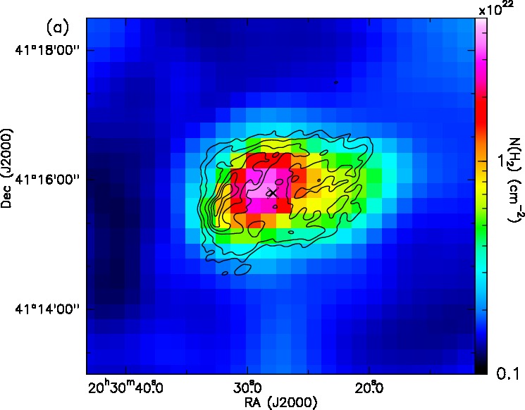
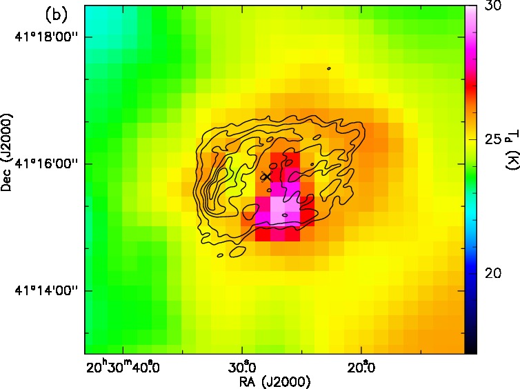
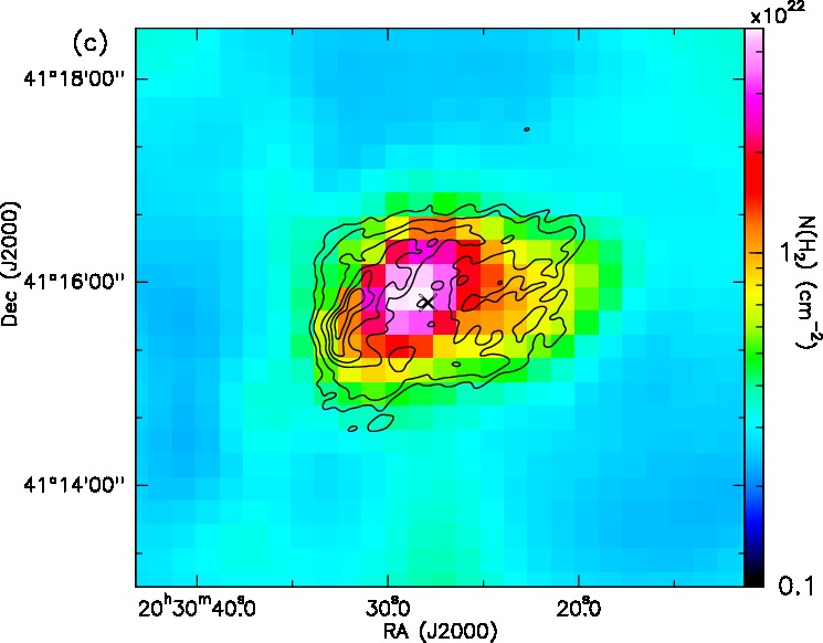
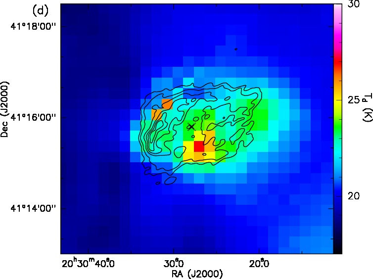
Figure 12: (a) Column density and (b) dust temperature map in the region associated with IRAS 20286+4105 derived from modified black body fitting using 70 - 500 $\rm\mu m$ data . Overlaid on the images are the low resolution 1280 MHz radio contours. The contour levels are 3, 5, 10, 15, 20, 25 times $\sigma$ (0.187 mJy/beam). The $\times$ shows the position of the IRAS point source. (c) and (d) are same as (a) and (b), respectively but excluding 70 $\rm\mu m$ emission in the modified black body modeling.

We co-relate the emission to a modified blackbody that takes into consideration the optical depth, and the dust emissivity. This is done pixel wise using the following expression (Ward-Thompson & Robson, 1990; Faimali et al., 2012; Pitann et al., 2013; Mallick et al., 2015),

$$S_{\nu}(\nu)-I_{\rm bkg}(\nu)=B_{\nu}(\nu,T_{d})\Omega(1-e^{-\tau_{\nu}})$$ (8)

where, $S_{\nu}(\nu)$ is the observed flux density, $I_{\rm bkg}(\nu)$ is the background flux which in our case is obtained from the Gaussian fit, $B_{\nu}(\nu,T_{d})$ is the Planck’s function, $T_{d}$ is the dust temperature, $\Omega$ is the solid angle (in steradians) from where the flux is obtained (solid angle subtended by a 14${}^{\prime\prime}\times$ 14^′′ pixel) and $\tau_{\nu}$ is the optical depth. The optical depth in turn is given by,

$$\tau_{\nu}=\mu_{\rm H_{2}}m_{\rm H}\kappa_{\nu}N(\rm H_{2})$$ (9)

where, $\mu_{\rm H_{2}}$ is the mean molecular weight, $m_{\rm H}$ is the mass of hydrogen atom, $\kappa_{\nu}$ is the dust opacity and $N(\rm H_{2}$) is the column density. We assume a value of 2.8 for $\mu_{\rm H_{2}}$ (Kauffmann et al., 2008). The dust opacity $\kappa_{\nu}$ is defined to be $\kappa_{\nu}=0.1~{}(\nu/1000~{}{\rm GHz})^{\beta}~{}{\rm cm^{2}/g}$. $\beta$ is the dust emissivity spectral index which is assumed to be 2 (Hildebrand, 1983; Beckwith et al., 1990; André et al., 2010). The non-linear least square Levenberg-Marquardt fitting algorithm is used. We include 15% uncertainty in the background subtracted Hi-GAL fluxes (Launhardt et al. 2013). Dust temperature and column density are taken as free parameters in the model. From the fitted values, the temperature and column density maps are generated.

According to Compiègne et al. (2010), the contribution from the stochastically heated very small grains (radius $<$ 0.005 $\mu$m) to the PACS 70 $\mu$m channel can be as large as $\sim$50%. Hence, a single modified blackbody model fit would possibly overestimate the cold dust temperatures and a two-temperature gray body is therefore essential to represent the emission from 70 $\mu$m (Galametz et al., 2012). Several studies have excluded the 70 $\rm\mu m$ (Battersby et al., 2011; Sadavoy et al., 2012) while generating the above maps. However, we present maps with and without 70 $\rm\mu m$ emission and investigate the effect of this waveband on the modeled column density and dust temperature distribution.

Figure 12 shows the column density and dust temperature distribution of the region associated with IRAS 20286+4105. In the figure we have maintained same scaling for images with and without 70 $\rm\mu m$ emission for ease of comparison. The morphology is similar in both the column density maps with a single clump which traces the IRAS 20286+4105 cloud. The densest part of the cloud is seen to be coincident with the position of the IRAS point source. However, the pixels in the map generated without 70 $\rm\mu m$ flux fit to higher values. The median of the fitted column density values are $\rm 1.6\times 10^{21}\,cm^{-2}$ and $\rm 2.9\times 10^{21}\,cm^{-2}$ with and without 70 $\rm\mu m$ flux, respectively. In comparison, the morphology changes in the temperature maps where the one generated without 70 $\rm\mu m$ emission displays a relatively elongated distribution. Here, the pixels in the map generated by including the 70 $\rm\mu m$ fits to higher temperatures as expected and discussed earlier. The median of the fitted dust temperature values are 24.6 K and 19.9 K with and without 70 $\rm\mu m$ data, respectively.

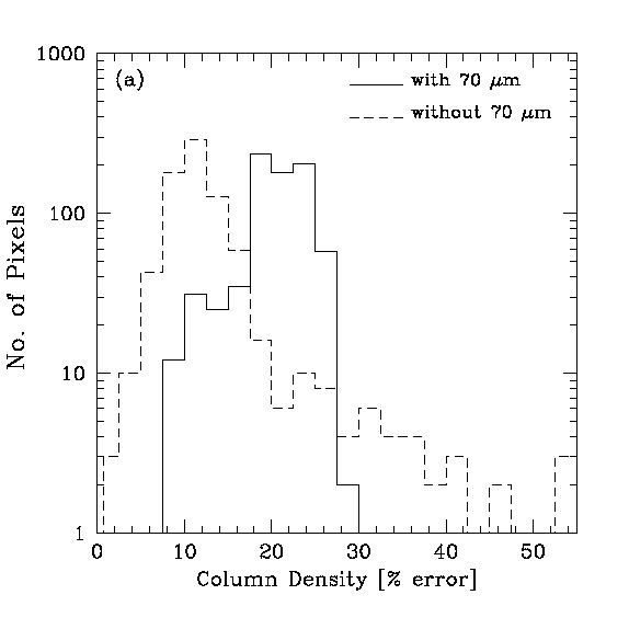
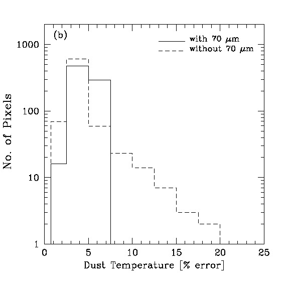
Figure 13: Histograms pixel distribution of the percentage error in the fitted values for (a) Column density and (b) Dust temperature. The solid and dashed lines are including and excluding 70 $\rm\mu m$ emission, respectively.

For deriving the physical parameters, we inspect the fitting errors in both set of maps. In Figure 13, we plot the pixel distribution of the percentage errors on the fitted values for the generated maps shown in Figure 12. As is evident, the percentage errors in the column density maps peak at lower values if we exclude 70 $\rm\mu m$ flux with the median error in the derived column density being $\sim$ 20 and 12% with and without 70 $\rm\mu m$ data, respectively. However, the percentage error reaches as high values as 55% if we exclude 70 $\rm\mu m$ emission. In addition, all the pixels having fitting errors above 20% lie inside the IRAS 20286+4105 cloud. This amounts to half the pixels of the cloud. Whereas, the percentage of such ‘bad’ pixels reduces to only 10% if we include all five Herschel bands. The errors in both the temperature maps are below 20%, with the median error in the derived dust temperature being $\sim$ 5 and 4% with and without 70 $\rm\mu m$ flux, respectively. Hence, for mass estimation (see next section), we use the maps generated including the 70 $\rm\mu m$ data point.

3.5.2 Properties of dust clumps

The low resolution of the column density maps restrain us in resolving sub-clumps, if any, within this central clump. Hence, we use the 250 $\rm\mu m$ image and the 2D variation of the clumpfind algorithm (Williams, de Geus & Blitz, 2011) to detect and identify sub-clumps. The 250 $\rm\mu m$ image has a higher and optimum resolution of 18″. A threshold contour level of 630 MJy/Sr (which corresponds to $\rm 18\sigma$) is used with a contour spacing of $\rm 3\sigma$. The rms noise of the map, $\sigma$, is estimated to be 35 MJy/Sr . The two sub-clumps identified using the 250 $\rm\mu m$ image are shown in Figure 14.

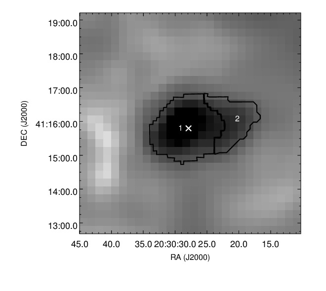
Figure 14: Clump apertures identified using clumpfind algorithm marked over the derived column density map shown in Figure 12.

Masses of these two clumps associated with IRAS 20286+4105 are estimated from the derived column density map using the following expression from Nielbock et al. (2012).

$$\rm M_{clump}=\mu_{\rm H_{2}}m_{\rm H}A_{\rm pixel}\Sigma{\it N}(\rm H_{2})$$ (10)

where m_H is the mass of hydrogen, A_pixel is the pixel area in cm², $\mu_{\rm H_{2}}$ is the mean molecular weight and $\rm\Sigma{\it N}(H_{2})$ is the integrated column density over the pixel area. The clump apertures retrieved from the clumpfind algorithm are used to obtain the integrated column density. Masses of Clump 1 and 2 are estimated to be $\sim$ 173 and 30 $\rm M_{\odot}$, respectively.

We also determine the masses of the sub-clumps from the 250 $\rm\mu m$ image using the following expression from Kauffmann et al. (2008),

$$\rm M=0.12~{}\rm M_{\odot}\left(e^{1.439(\lambda/{\rm mm})^{-1}({\it T}_{\it d}/10K)^{-1}}-1\right)$$ (11)

$$\times\left(\frac{{\kappa}_{\nu}}{\rm 0.01cm^{2}g^{-1}}\right)^{-1}\left(\frac{S_{\nu}}{\rm Jy}\right)\left(\frac{D}{\rm 100pc}\right)^{2}\left(\frac{\lambda}{\rm mm}\right)^{3}$$

where $T_{d}$ is the dust temperature, ${\kappa}_{\nu}$ is the dust opacity which is taken as $0.1(\frac{\nu}{\rm 1000GHz})^{\beta}$, D is the distance, $S_{\nu}$ is the integrated flux. $T_{d}$ is assumed to be the median value of the dust temperature within the aperture of the clumps. The derived masses and other physical properties of the clumps are listed in Table 4. The volume densities, $n_{\rm H_{2}}$, are estimated assuming spherical clumps of uniform density. Masses derived using the column density maps are on the lower side compared to those derived from the 250 $\rm\mu m$ fluxes. We adopt the former values since these are determined using all five Herschel images and hence would be a better estimate. The total mass of the clumps associated with IRAS 20286+4105 is 203 M_⊙ which is higher as compared to the estimate of 160 M_⊙ obtained by Roy et al. (2011) using data from the BLAST survey. It should be noted here that the effective radius used by them is lower (0.5 pc) compared to our combined clump size.

Table 4: Physical properties of the clumps.

Clump No	Dust Temp.	Effective Radius	$n_{\rm H_{2}}$	Clump Mass	Clump Mass
				(from 250 $\rm\mu m$)	(from column density map)
	(K)	(pc)	($\rm\times 10^{3}cm^{-3}$)	(M⊙)	(M${}_{\odot})$
1	25.7	0.47	5.8	197	173
2	25.8	0.34	2.7	40	30

Clump 1 has tracers of ongoing star formation. It is seen to be associated with intermediate-mass stars, masers, 24 $\rm\mu m$ emission from warm dust and outflows. All the six identified candidate YSOs are located within Clump 1. Except an arc of faint 24 $\rm\mu m$ emission, Clump 2 does not show any signature of active star formation region and hence seems to be a potential new site for future generation of star formation.

3.5.3 Variation in Dust Emissivity Index

There is growing evidence of an inverse relationship between the dust emissivity spectral index, $\beta$ and the dust temperature, $T_{d}$ (Dupac et al., 2003; Désert et al., 2008; Paradis et al., 2010; Veneziani et al., 2010; Anderson et al., 2012). We investigate this for the region associated with IRAS 20286+4105. Temperature maps are generated for two additional values of $\beta$ = 1.5 and 2.5. The histograms of the dust temperature maps are shown in Figure 15. Here, pixels having error less than 20% on the fitted temperature values are chosen. From the histograms, an inverse relation of $\beta$ with the dust temperature is evident. The peak of the distribution shifts to lower temperatures as $\beta$ increases.

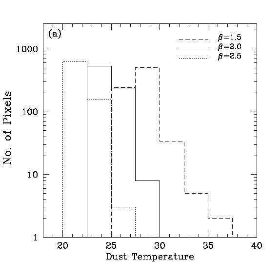
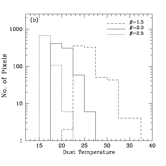
Figure 15: Histogram of pixels values for dust temperature from maps generated with three fixed values of $\beta=1.5,2.0,2.5$ (a) including 70 $\rm\mu m$ flux and (b) excluding 70 $\rm\mu m$ flux.

Next we keep $\beta$ as a free parameter along with temperature and column density in the model. We proceed further for a pixel wise analysis of the generated $\beta$ and dust temperature maps. This enables us to probe the correlation between these two parameters in the vicinity of a star forming region at a resolution of 36^′′. We select only those pixels from our $\beta$ and $T_{d}$ maps which have errors less than 20% in both parameter space. This procedure is inspired from the work of Dupac et al. (2003), who explain the existence of a degeneracy between these two quantities which is due to the inherent large error bars on $\beta$ for colder regions and large errors for temperature for warmer components. Figure 16 plots the pixel values of $\beta$ as a function of the dust temperature for a $\rm 5\arcmin\times 5\arcmin~{}$ region centered on the IRAS point source. It should be noted here that in the maps generated, without the 70 $\rm\mu m$ data, a single pixel was found with errors in both parameters less than 5% but a high fitted value of temperature ($\sim 69$ K) and a low value of $\beta$ ($\sim 0.7$). In Figure 16, we also show fits from other studies showing the relation between these two parameters. The values of $\beta$ and $T_{d}$ obtained from the maps generated including the 70 $\rm\mu m$ emission hints at the inverse relation whereas, the values obtained without including the 70 $\rm\mu m$ emission clearly shows an inverse correlation between the dust emissivity index and the temperature. As discussed earlier, including 70 $\rm\mu m$ emission possibly overestimates the cold dust temperature and this could be the reason for the above difference seen. The result obtained in the latter case is consistent with the best fit curve estimated by Paradis et al. (2010). The lower temperature region is also well correlated with the above fit. Their results are based on two Hi-GAL fields at Galactic longitudes, $l=30^{\circ}$ and $l=59^{\circ}$. There is a high density of points in the temperature range $\sim 22-35$ K, where a significant number of pixels seem to follow the fit proposed by Désert et al. (2008). Their results are based on submillimetre point sources from the Archeops experiment. As discussed in Veena et al. (2015) and references therein, this anti-correlation is attributed to the intrinsic properties of the grains in the cold dust environments. The warmer regions can be understood as comprising of low emissivity index bare silicate aggregates or porous graphite grains (Dupac et al., 2003; Mathis & Whiffen, 1989), while the regions with higher $\beta$ values could have the composition of icy mantles (Aannestad, 1975).

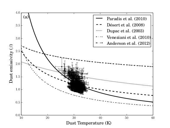
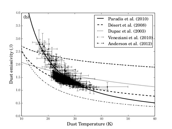
Figure 16: Variation of $\beta$ with dust temperature for a $\rm 5\arcmin\times 5\arcmin~{}$ region centered on the IRAS point source. (a) Plot from maps including 70 $\rm\mu m$ flux and (b) Plot from maps excluding 70 $\rm\mu m$ emission. Fits from literature (Dupac et al., 2003; Désert et al., 2008; Paradis et al., 2010; Veneziani et al., 2010; Anderson et al., 2012) are shown.

3.6 General star formation scenario in IRAS 20286+4105

The ‘runaway’ star hypothesis suggests that the massive B0 - B0.5 star responsible for the ionized emission is not formed from the IRAS 20286+4105 cloud but instead has its birthplace in the supernova remnant. The ongoing star formation activity in this cloud thus includes the six Class I sources seen clustered towards the cloud centre. The SED modelling of these indicate that five of them are intermediate mass stars. In the absence of massive stars, the bright 24 $\rm\mu m$ MIR emission is mostly due to this cluster of intermediate-mass Class I sources. This however does not preclude the presence of further deeply embedded young protostars contributing towards heating the dust which radiates at 24 $\rm\mu m$. The total luminosity of the six sources add up to $\rm\sim 10^{3}L_{\odot}$ which is an appreciable fraction of the total luminosity of 5.3 $\times 10^{3}$ L_⊙ cited earlier. Thus, there seems to be no conclusive evidence of high-mass star formation in this cloud.

The above discussion finds support in the nature of Clump 1 which hosts the embedded sources. For the estimated radius of 0.5 pc, the mass should be greater than $\rm\sim 320\,M_{\odot}$ for the clump to form high-mass stars (Kauffmann & Pillai, 2010). This is almost twice the value estimated from the column density map. Hence, following the empirical mass-radius relation given by Kauffmann & Pillai (2010), this clump should be devoid of massive stars. So is the case with Clump 2 for which the threshold mass is calculated to be $\rm\sim 210\,M_{\odot}$ which is almost seven times higher than that estimated from the Herschel maps. Another criterion for clumps to be high-mass star forming sites was proposed by Krumholz & McKee (2008), who predicted a threshold surface density ($\Sigma_{th}$) of $\rm\sim 1\,g\,cm^{-2}$ for massive stars to form as opposed to fragmentation into lower masses. The estimated values of $\Sigma$ for Clumps 1 and 2 are 0.05 and 0.02 $\rm g\,cm^{-2}$, respectively. The estimate of Clump 1 is marginally lower than the value of 0.117 $\rm g\,cm^{-2}$ determined by Roy et al. (2011). These estimated $\Sigma$ values are far below $\Sigma_{th}$ = 1. In a detailed study of massive star forming cores, Chambers et al. (2009) have shown that only for a small fraction cores $\Sigma>\Sigma_{th}$ and the median values of both active and quiescent cores are $\rm\sim 0.2\,g\,cm^{-2}$. As discussed by these authors, the low values of $\Sigma$ could be attributed to the large clump apertures adopted and the actual core mass densities could be higher and possibly closer to $\Sigma_{th}$. However, a point worth noting here is that, for both the clumps associated with IRAS 20286+4105, the $\Sigma$ values are $\sim 5-13$ lower than the values estimated for active and quiescent cores by Chambers et al. (2009). Thus, given the mass threshold and the surface mass density estimates, the picture of a runaway star and triggered population of intermediate-mass Class I objects augurs well with the physical condition of the clumps which do not qualify as massive star forming sites.

4 Conclusion

In this paper we carried out an extensive multi-wavelength study of the star forming region IRAS 20286+4105 and its associated environment. Our main inferences are as follows

1. Using UKIDSS NIR data, we show the effect of sensitivity on the detection of sparsely populated clusters. The 2MASS cluster known to be associated with IRAS 20286+4105 is not detected with the deeper UKIDSS data. This could possibly be due to the overwhelming background sampled which suppresses this low stellar density cluster/group.

2. As deduced from the MIR and NIR data, the region is an active star forming complex harboring a cluster of six Class I YSOs towards the center of the cloud. SED modeling indicates the YSOs to be mostly intermediate mass stars. Several detected masers are seen to be located in the close vicinity of these Class I sources.

3. GMRT radio continuum observations at 610 and 1280 MHz in conjunction with VLA 4.89 GHz archival data show the presence of a cometary HII region consistent with the morphology obtained for ionized gas in optical (H$\alpha$) and NIR (Br$\gamma$). Assuming optically thin free-free emission, the spectral type of a single ionizing star responsible for this is estimated to be B0.5 - B0.

4. The bow-shock model seems to be the likely mechanism responsible for the cometary radio morphology. The projected stand-off distances at 1.61 kpc are estimated to lie between $\sim$ 2″- 13″, which indicate that the ionizing source lies within the radio arc. If we assume the radio peak to be associated with the ionizing source then the stand-off distance is consistent with the distance of the edge of the radio arc from the radio peak position. The above argument of the bow-shock model finds support in the morphological indication of a possible association with a supernova remnant SNR G079.8+1.2 which might be responsible for the supersonic motion of the ionizing star. Kinematic age estimate of the runaway star responsible for the bow-shock supports the binary supernova scenario of high-velocity stars.

5. The Class I sources located inside the cloud could be a population formed due to the collapse of a pre-existing clump triggered by an encroaching shock associated with the supernova. Further evidence of triggered star formation is seen as an enhanced density of YSOs towards the east and bordering the radio arc.

6. Apart from the diffuse emission, we detect a radio knot (RS1) which shows a negative spectral index ($\rm\sim-0.5\pm 0.05$). This knot is seen to be coincident with the position of an outflow and hence is likely to be due to the non-thermal emission associated with it.

7. From the FIR Herschel data, we generate the dust temperature and column density maps. The presence of a central dust clump is clearly seen in the column density map. Using the 250 $\rm\mu m$ and the 2D variation of the clumpfind algorithm, this central clump is resolved into two sub-clumps with estimated masses from the column density maps to be 173$\,{\rm M}_{\odot}$ (Clump 1) and 30$\,{\rm M}_{\odot}$ (Clump 2).

8. Clump 1 is seen to be an active star forming region, whereas Clump 2 shows no sign of ongoing star formation.

9. The mass, radius and surface density of the clumps indicate that they are likely to be devoid of massive star formation.

10. We investigate the relation between the dust temperature and the dust emissivity spectral index in the vicinity of the IRAS 20286+4105 star forming complex. Variation is seen in the spectral index which shows an anti-correlation with dust temperature.

Acknowledgment : We would like to thank the referee for his/her valuable suggestions which helped in improving the quality of the paper. VR would like to thank Dr. Ishwara Chandra of NCRA, Pune for organizing a workshop for introduction to radio data analysis. We thank the staff of the GMRT, that made the radio observations possible. GMRT is run by the National Centre for Radio Astrophysics of the Tata Institute of Fundamental Research. We thank the staff of IAO, Hanle and CREST, Hosakote, that made the NIR observations possible. The facilities at IAO and CREST are operated by the Indian Institute of Astrophysics, Bangalore.

References

- Aannestad (1975) Aannestad P. A., 1975, \apj, 200, 30
- Alakoz et al. (2002) Alakoz A. V., Kalenskii S. V., Promislov V. G., Johansson L. E. B., Winnberg A., 2002, Astronomy Reports, 46, 551
- Allen et al. (2004) Allen L. E. et al., 2004, \apjs, 154, 363
- Anderson et al. (2012) Anderson L. D. et al., 2012, \aap, 542, A10
- André et al. (2010) André P. et al., 2010, \aap, 518, L102
- Battersby et al. (2011) Battersby C. et al., 2011, \aap, 535, A128
- Beckwith et al. (1990) Beckwith S. V. W., Sargent A. I., Chini R. S., Guesten R., 1990, \aj, 99, 924
- Blaauw (1961) Blaauw A., 1961, \bain, 15, 265
- Brand & Blitz (1993) Brand J., Blitz L., 1993, \aap, 275, 67
- Brand et al. (1994) Brand J. et al., 1994, \aaps, 103, 541
- Bronfman, Nyman & May (1996) Bronfman L., Nyman L.-A., May J., 1996, \aaps, 115, 81
- Casertano & Hut (1985) Casertano S., Hut P., 1985, \apj, 298, 80
- Chambers et al. (2009) Chambers E. T., Jackson J. M., Rathborne J. M., Simon R., 2009, \apjs, 181, 360
- Chavarría et al. (2008) Chavarría L. A., Allen L. E., Hora J. L., Brunt C. M., Fazio G. G., 2008, \apj, 682, 445
- Codella, Felli & Natale (1996) Codella C., Felli M., Natale V., 1996, \aap, 311, 971
- Comerón & Torra (2001) Comerón F., Torra J., 2001, \aap, 375, 539
- Compiègne et al. (2010) Compiègne M., Flagey N., Noriega-Crespo A., Martin P. G., Bernard J.-P., Paladini R., Molinari S., 2010, \apjl, 724, L44
- Crusius-Wätzel (1993) Crusius-Wätzel A. R., 1993, in Astrophysics and Space Science Library, Vol. 186, Stellar Jets and Bipolar Outflows, Errico L., Vittone A. A., eds., p. 311
- de Buizer et al. (2005) de Buizer J. M., Radomski J. T., Telesco C. M., Piña R. K., 2005, in IAU Symposium, Vol. 227, Massive Star Birth: A Crossroads of Astrophysics, Cesaroni R., Felli M., Churchwell E., Walmsley M., eds., pp. 180–185
- Deharveng et al. (2000) Deharveng L., Peña M., Caplan J., Costero R., 2000, \mnras, 311, 329
- Désert et al. (2008) Désert F.-X. et al., 2008, \aap, 481, 411
- Dupac et al. (2003) Dupac X. et al., 2003, \aap, 404, L11
- Dutra & Bica (2001) Dutra C. M., Bica E., 2001, \aap, 376, 434
- Dye et al. (2006) Dye S. et al., 2006, \mnras, 372, 1227
- Edris, Fuller & Cohen (2007) Edris K. A., Fuller G. A., Cohen R. J., 2007, \aap, 465, 865
- Faimali et al. (2012) Faimali A. et al., 2012, \mnras, 426, 402
- Finch & Zacharias (2016) Finch C. T., Zacharias N., 2016, \aj, 151, 160
- Galametz et al. (2012) Galametz M. et al., 2012, \mnras, 425, 763
- Gan et al. (2013) Gan C.-G., Chen X., Shen Z.-Q., Xu Y., Ju B.-G., 2013, \apj, 763, 2
- Gies & Bolton (1986) Gies D. R., Bolton C. T., 1986, \apjs, 61, 419
- González-Solares et al. (2008) González-Solares E. A. et al., 2008, \mnras, 388, 89
- Gutermuth et al. (2008) Gutermuth R. A. et al., 2008, \apj, 674, 336
- Haslam et al. (1982) Haslam C. G. T., Salter C. J., Stoffel H., Wilson W. E., 1982, \aaps, 47, 1
- Haverkorn, Katgert & de Bruyn (2003) Haverkorn M., Katgert P., de Bruyn A. G., 2003, \aap, 403, 1031
- Hildebrand (1983) Hildebrand R. H., 1983, \qjras, 24, 267
- Hoogerwerf, de Bruijne & de Zeeuw (2001) Hoogerwerf R., de Bruijne J. H. J., de Zeeuw P. T., 2001, \aap, 365, 49
- Hora et al. (2007) Hora J. et al., 2007, A Spitzer Legacy Survey of the Cygnus-X Complex. Spitzer Proposal
- Israel (1978) Israel F. P., 1978, \aap, 70, 769
- Kauffmann et al. (2008) Kauffmann J., Bertoldi F., Bourke T. L., Evans, II N. J., Lee C. W., 2008, \aap, 487, 993
- Kauffmann & Pillai (2010) Kauffmann J., Pillai T., 2010, \apjl, 723, L7
- Krumholz & McKee (2008) Krumholz M. R., McKee C. F., 2008, \nat, 451, 1082
- Kumar, Keto & Clerkin (2006) Kumar M. S. N., Keto E., Clerkin E., 2006, \aap, 449, 1033
- Kumar, Ojha & Davis (2003) Kumar M. S. N., Ojha D. K., Davis C. J., 2003, \apj, 598, 1107
- Lada (1987) Lada C. J., 1987, in IAU Symposium, Vol. 115, Star Forming Regions, Peimbert M., Jugaku J., eds., pp. 1–17
- Lada & Lada (1995) Lada E. A., Lada C. J., 1995, \aj, 109, 1682
- Launhardt et al. (2013) Launhardt R. et al., 2013, \aap, 551, A98
- Lawrence et al. (2007) Lawrence A. et al., 2007, \mnras, 379, 1599
- Lu et al. (2014) Lu X., Zhang Q., Liu H. B., Wang J., Gu Q., 2014, \apj, 790, 84
- Lucas et al. (2008) Lucas P. W. et al., 2008, \mnras, 391, 136
- Mac Low et al. (1991) Mac Low M.-M., van Buren D., Wood D. O. S., Churchwell E., 1991, \apj, 369, 395
- Mallick et al. (2015) Mallick K. K., Ojha D. K., Tamura M., Linz H., Samal M. R., Ghosh S. K., 2015, \mnras, 447, 2307
- Marcote et al. (2015) Marcote B., Ribó M., Paredes J. M., Ishwara-Chandra C. H., 2015, \mnras, 451, 59
- Marti, Rodriguez & Reipurth (1993) Marti J., Rodriguez L. F., Reipurth B., 1993, \apj, 416, 208
- Martín-Hernández, van der Hulst & Tielens (2003) Martín-Hernández N. L., van der Hulst J. M., Tielens A. G. G. M., 2003, \aap, 407, 957
- Mathis & Whiffen (1989) Mathis J. S., Whiffen G., 1989, \apj, 341, 808
- McCutcheon et al. (1991) McCutcheon W. H., Sato T., Dewdney P. E., Purton C. R., 1991, \aj, 101, 1435
- Megeath et al. (2004) Megeath S. T. et al., 2004, \apjs, 154, 367
- Moffat et al. (1998) Moffat A. F. J. et al., 1998, \aap, 331, 949
- Molinari et al. (1996) Molinari S., Brand J., Cesaroni R., Palla F., 1996, \aap, 308, 573
- Molinari et al. (2010) Molinari S. et al., 2010, \aap, 518, L100
- Mottram et al. (2011) Mottram J. C. et al., 2011, \apjl, 730, L33
- Nielbock et al. (2012) Nielbock M. et al., 2012, \aap, 547, A11
- Ninan et al. (2014) Ninan J. P. et al., 2014, Journal of Astronomical Instrumentation, 3, 50006
- Odenwald & Schwartz (1989) Odenwald S. F., Schwartz P. R., 1989, \apjl, 345, L47
- Ojha et al. (2012) Ojha D. K. et al., 2012, in Astronomical Society of India Conference Series, Vol. 4, Astronomical Society of India Conference Series, p. 191
- Ojha et al. (2004) Ojha D. K. et al., 2004, \apj, 608, 797
- Palla et al. (1991) Palla F., Brand J., Comoretto G., Felli M., Cesaroni R., 1991, \aap, 246, 249
- Panagia (1973) Panagia N., 1973, \aj, 78, 929
- Paradis et al. (2010) Paradis D. et al., 2010, \aap, 520, L8
- Parthasarathy, Jain & Bhatt (1992) Parthasarathy M., Jain S. K., Bhatt H. C., 1992, \aap, 266, 202
- Pitann et al. (2013) Pitann J. et al., 2013, \apj, 766, 68
- Poveda, Ruiz & Allen (1967) Poveda A., Ruiz J., Allen C., 1967, Boletin de los Observatorios Tonantzintla y Tacubaya, 4, 86
- Reid et al. (1995) Reid M. J., Argon A. L., Masson C. R., Menten K. M., Moran J. M., 1995, \apj, 443, 238
- Reid & Ho (1985) Reid M. J., Ho P. T. P., 1985, \apjl, 288, L17
- Robitaille et al. (2007) Robitaille T. P., Whitney B. A., Indebetouw R., Wood K., 2007, \apjs, 169, 328
- Robitaille et al. (2006) Robitaille T. P., Whitney B. A., Indebetouw R., Wood K., Denzmore P., 2006, \apjs, 167, 256
- Rodriguez et al. (1993) Rodriguez L. F., Marti J., Canto J., Moran J. M., Curiel S., 1993, \rmxaa, 25, 23
- Roy et al. (2011) Roy A. et al., 2011, \apj, 727, 114
- Sadavoy et al. (2012) Sadavoy S. I. et al., 2012, \aap, 540, A10
- Schmeja (2011) Schmeja S., 2011, Astronomische Nachrichten, 332, 172
- Schmeja, Kumar & Ferreira (2008) Schmeja S., Kumar M. S. N., Ferreira B., 2008, \mnras, 389, 1209
- Schneider et al. (2006) Schneider N., Bontemps S., Simon R., Jakob H., Motte F., Miller M., Kramer C., Stutzki J., 2006, \aap, 458, 855
- Setia Gunawan et al. (2003) Setia Gunawan D. Y. A., de Bruyn A. G., van der Hucht K. A., Williams P. M., 2003, \apjs, 149, 123
- Shirley et al. (2013) Shirley Y. L. et al., 2013, \apjs, 209, 2
- Simon et al. (2007) Simon J. D. et al., 2007, \apj, 669, 327
- Skrutskie et al. (2006) Skrutskie M. F. et al., 2006, \aj, 131, 1163
- Swarup (1991) Swarup G., 1991, in Astronomical Society of the Pacific Conference Series, Vol. 19, IAU Colloq. 131: Radio Interferometry. Theory, Techniques, and Applications, Cornwell T. J., Perley R. A., eds., pp. 376–380
- Tej et al. (2006) Tej A., Ojha D. K., Ghosh S. K., Kulkarni V. K., Verma R. P., Vig S., Prabhu T. P., 2006, \aap, 452, 203
- Tenorio-Tagle (1979) Tenorio-Tagle G., 1979, \aap, 71, 59
- Urquhart et al. (2011) Urquhart J. S. et al., 2011, \mnras, 418, 1689
- van Buren & Mac Low (1992) van Buren D., Mac Low M.-M., 1992, \apj, 394, 534
- van Buren et al. (1990) van Buren D., Mac Low M.-M., Wood D. O. S., Churchwell E., 1990, \apj, 353, 570
- van Buren & McCray (1988) van Buren D., McCray R., 1988, \apjl, 329, L93
- van der Walt, Gaylard & MacLeod (1995) van der Walt D. J., Gaylard M. J., MacLeod G. C., 1995, \aaps, 110, 81
- Varricatt et al. (2010) Varricatt W. P., Davis C. J., Ramsay S., Todd S. P., 2010, \mnras, 404, 661
- Veena et al. (2015) Veena V. S., Vig S., Tej A., Varricatt W. P., Ghosh S. K., Chandrasekhar T., Ashok N. M., 2015, ArXiv e-prints
- Veneziani et al. (2010) Veneziani M. et al., 2010, \apj, 713, 959
- Verma et al. (2003) Verma R. P., Ghosh S. K., Mookerjea B., Rengarajan T. N., 2003, \aap, 398, 589
- Vig et al. (2007) Vig S., Ghosh S. K., Ojha D. K., Verma R. P., 2007, \aap, 463, 175
- Vig et al. (2014) Vig S., Ghosh S. K., Ojha D. K., Verma R. P., Tamura M., 2014, \mnras, 440, 3078
- Ward-Thompson & Robson (1990) Ward-Thompson D., Robson E. I., 1990, \mnras, 244, 458
- Wendker (1984) Wendker H. J., 1984, \aaps, 58, 291
- Wendker, Higgs & Landecker (1991) Wendker H. J., Higgs L. A., Landecker T. L., 1991, \aap, 241, 551
- Williams, de Geus & Blitz (2011) Williams J. P., de Geus E. J., Blitz L., 2011, Clumpfind: Determining Structure in Molecular Clouds. Astrophysics Source Code Library
- Wood & Churchwell (1989) Wood D. O. S., Churchwell E., 1989, \apjs, 69, 831
- Xu et al. (2013) Xu Y. et al., 2013, \apj, 769, 15
- Xue et al. (2008) Xue X. et al., 2008, The Astrophysical Journal, 684, 1143
- Zhang et al. (2005) Zhang Q., Hunter T. R., Brand J., Sridharan T. K., Cesaroni R., Molinari S., Wang J., Kramer M., 2005, \apj, 625, 864