Gaussian process regression can turn non-uniform and undersampled diffusion MRI data into diffusion spectrum imaging
Abstract
We propose to use Gaussian process regression to accurately estimate the diffusion MRI signal at arbitrary locations in q-space. By estimating the signal on a grid, we can do synthetic diffusion spectrum imaging: reconstructing the ensemble averaged propagator (EAP) by an inverse Fourier transform. We also propose an alternative reconstruction method guaranteeing a nonnegative EAP that integrates to unity. The reconstruction is validated on data simulated from two Gaussians at various crossing angles. Moreover, we demonstrate on non-uniformly sampled in vivo data that the method is far superior to linear interpolation, and allows a drastic undersampling of the data with only a minor loss of accuracy. We envision the method as a potential replacement for standard diffusion spectrum imaging, in particular when acquistion time is limited.
Index Terms— Diffusion MRI, Diffusion Spectrum Imaging, Gaussian processes, machine learning
1 Introduction
The structure of biological tissue affects the diffusion of particles within it. The diffusion MRI signal stems from the translational motion of spin-bearing particles—water in particular—and can thus be used to probe the tissue structure.
The voxel-averaged distribution of spins’ displacement is referred to as the ensemble averaged propagator (EAP). Although the imaging voxel is macroscopic, the characteristic length-scale of the translational motion in a typical diffusion MRI experiment is commensurate with cell dimensions. This makes the EAP an indirect but potentially powerful way of describing the diffusion behavior in complex materials [1]. For example, the EAP can be used to characterize the tissue using various scalar indices [1, 2, 3]. It can also be used in tractography by mapping the EAP to an orientation density function (ODF) through a radial projection [4]. This enables the whole arsenal of tractography algorithms developed for High Angular Resolution Diffusion Imaging (HARDI) [5].
Under the narrow pulse approximation [6], there is a direct Fourier relationship [7] between the normalized diffusion signal, , in q-space and the EAP, denoted , in real space
| (1) |
where is the displacement vector and is the diffusion signal measured at q-space point . Here, is the gyromagnetic ratio and is the duration of the diffusion sensitizing gradients whose magnitude and orientation are determined by the vector . Diffusion Spectrum Imaging (DSI) [8] is the direct application of equation (1): measurements are done on a dense Cartesian grid in q-space, after which the EAP is found by an inverse 3D Fourier transform. However, this requires such a large number of q-space samples that the acquisition time becomes too long for routine use.
We describe how to use a machine learning method called Gaussian process regression to estimate the q-space signal based on far fewer samples than required by DSI. In particular, we show how to resample data acquired on multiple shells (radii) onto a Cartesian grid. Although an estimate of the EAP could then be obtained by an inverse Fast Fourier Transform, we also describe a theoretically well-founded reconstruction method that respects the probabilistic nature of the EAP.
Other researchers have also tackled this problem. One approach is to expand the q-space signal in a suitably chosen basis, e.g. in Hermite functions [2] or using a mixture of radial basis functions densely distributed in q-space [3]. Although both of these can in theory approximate any function to arbitrary accuracy, the finite number of samples in combination with the ever present noise, especially at large q-values, places severe restrictions on these models. Other methods require a particular sampling scheme, e.g. multiple concentric shells, after which some type of interpolation [9] or smoothing [10] can be used to estimate the intermediate values.
Adopting a Gaussian process framework, such as the one we propose, immediately gives access to an extensive set of tools that unite an elegant probabilistic view with computational tractability [11]. Notably, it enables expressive models yet has few parameters and it comes with a rigorous way of reasoning about uncertainty [12]. This work was inspired by previous work on using Gaussian processes to correct for artifacts in diffusion scans [13].
2 Theory
2.1 Gaussian process regression
A Gaussian process can be thought of as a Gaussian distribution over functions [11]. Just as a multivariate Gaussian distribution is fully specified by its mean and covariance matrix, a Gaussian process is fully described by its mean and covariance function. However, the mean function is typically set to zero because its effects can be absorbed in the covariance function. The covariance function tells us how similar two inputs are and thus how much they are allowed to influence each other. The evaluation of the covariance function at two points and is akin to the entry of a covariance matrix .
Now, let us describe how to use Gaussian processes for regressions provided that the mean and covariance functions are known. Suppose we have a training set composed of inputs and noisy measurement values generated from a latent function with i.i.d. Gaussian noise such that . Gaussian processes allow you to predict the function value at an arbitrary input point , as well as the corresponding variance (uncertainty if you will). If we organize the inputs as a matrix with rows and the function values as a vector , the joint distribution of the training data and the unobserved pair is given by
| (2) |
where is the matrix of covariances between all points in the training data, is the noise variance, is an vector of cross-covariances between the training data and the unobserved point . Finally, is the variance at the point . We use the convention that upper case signifies a matrix and bold font signifies a vector.
Using the standard identity for conditioning a Gaussian distribution [11], we find that the conditional probability of given , and is
| (3) | ||||
| (4) | ||||
| (5) |
2.2 A covariance function for diffusion MRI
There are several characteristics of the diffusion MRI signal that we would like to capture by an appropriate choice of covariance function. First, the signal is expected to be symmetric about the origin, i.e. . Second, we do not expect there to be any preferential directionality in the sense that the covariance between the signal when measuring in two directions should only depend on the angle between them. This suggests a factorization of the covariance into a radial part and an angular part such that
| (6) |
where and . In order for the angular part to be a valid covariance function on the sphere, we use the following theorem [14, 15]
Theorem 2.1.
A real continuous function is a valid covariance function on the sphere if and only if it is of the form
| (7) |
where , , and are the Legendre polynomials.
We take equal to the even terms of order in the above sum. Excluding odd terms guarantees symmetry about the origin, as desired.
We parameterized the radial part as
| (8) |
where is a constant used to make the function continuous in the origin. This is a valid kernel since it is the composition of a radial basis function with a function [12].
Taken together, we end up with six hyperparameters : four coefficients for the angular covariance (7), a length-scale of the radial covariance (8) and the noise variance . These are estimated by maximizing the marginal likelihood (so called empirical Bayes or type II maximum likelihood). Up to a constant, the logarithm of the marginal likelihood is given by [11]
| (9) |
where is the covariance matrix of the noisy measurements. If the voxels are assumed to be independent, then is block-diagonal: , where denotes the Kronecker product. This means that the marginal likelihood factorizes as
| (10) |
where is the set of all voxels. In practice, we perform the hyperparameter estimation on a large subset of all voxels and the testing on a different subset. Our implementation was made in MATLAB [16] using the Gaussian Processes for Machine Learning (GPML) toolbox [17].
2.3 Reconstruction of the ensemble averaged propagator
Recall from equation (1) that the ensemble averaged propagator (EAP) is the inverse Fourier transform of the normalized signal. A simple method for computing the EAP involves interpolating the signal onto a Cartesian grid and then applying a fast Fourier transform (FFT). However, this procedure does not guarantee that the resulting EAP estimate is nonnegative and integrates to unity. The quick and dirty solution for this is to set negative values to zero and then renormalize. We will however consider a better founded approach. In short, we readjust the estimated signal, using the variances of the Gaussian process estimates as weights, such that the inverse Fourier transform is nonnegative and integrates to unity.
The Gaussian process estimate at is where the mean and variance are given by equations (4) and (5) respectively. Since the predictions for different inputs are conditionally independent, the resulting log-likelihood is
| (11) |
where we have introduced a weight matrix .
The discrete inverse Fourier transform can be expressed as a matrix, which we denote . The constraint on nonnegative probability estimates can then be written simply as . To integrate to unity, it must hold that when . The nature of the diffusion signal requires it to be nonnegative, this is included as a bound. We thus end up with the following constrained weighted least-squares problem:
| (12) | ||||||
| subject to | ||||||
This is a convex quadratic programming problem which can be efficiently solved to global optimiality using e.g. an interior-point method.
2.4 Data augmentation
The Gaussian process model typically excels at interpolation and smoothing, whereas extrapolation poses more difficulties. To improve the extrapolation ability, we augment the data set with synthetic data at the origin (signal equal to one) and at a large radius where the signal is set to zero. Outside this cut-off radius, all signal estimates are set to zero. The data augmentation is done after training, so as to not affect the hyperparameters learned, but before prediction.
3 Results
3.1 Simulated data
We simulated data from two Gaussians of equal magnitude and equal but rotated diffusion tensors. As the unrotated diffusion tensor, we used , where m2/s. This yields a mean diffusivity (MD) of 1 m2/ms and a fractional anisotropy (FA) of 0.89, which is roughly the value observed in the white matter of the brain. The second diffusion tensor was determined by rotating by an angle about the z-axis, such that . The latent signal was thus
| (13) |
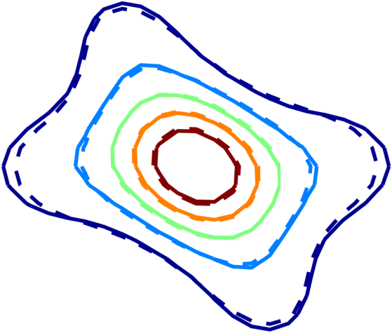
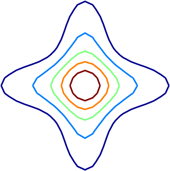
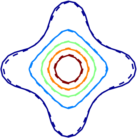
where ; here is the mixing time and the pulse duration. The latent signal was corrupted with Rician noise with scale parameter to yield the simulated signal. We used the same experimental parameters as in the the Human Connectome data described in the next section. The hyperparameters were optimized on a set of 100 Gaussian mixtures with randomly sampled crossing angles. Figure 1 compares exact and reconstructed EAPs for . We compare with using linear interpolation as in Hybrid Diffusion Imaging (HYDI) [9]. Table 1 shows the relative error in the estimation of the return-to-origin probability, , which is a scalar index indicative of the underlying structure.
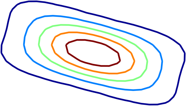
(a) Exact,
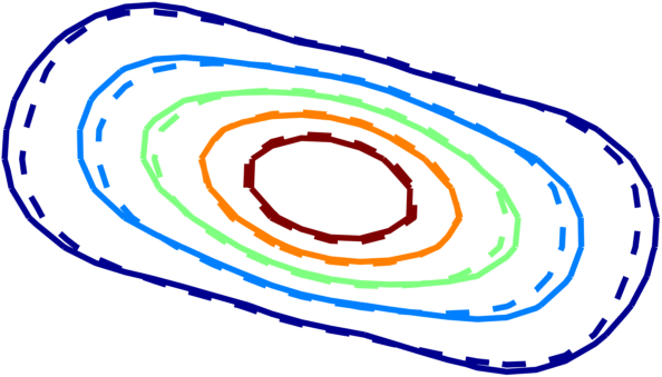
(b) Estimated,
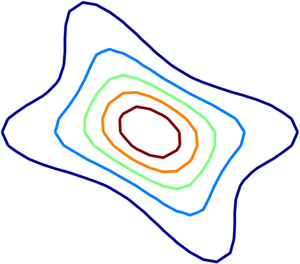
(a) Exact,
(b) Estimated,
(a) Exact,
(b) Estimated,
| This work | Linear interp. | |
|---|---|---|
| 0.036 | 0.058 | |
| 0.030 | 0.051 | |
| 0.027 | 0.050 |
3.2 Reconstruction of subsampled in vivo data
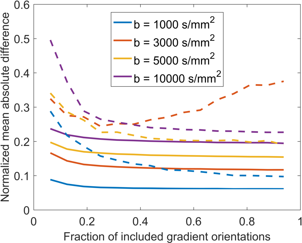
We used in vivo diffusion data obtained from the Human Connectome Project (HCP) [18] database111http://www.humanconnectome.org/documentation/MGH-diffusion/. The subjects are healthy adults, scanned on a customized Siemens 3T Connectom scanner [19, 20] using a Stejskal-Tanner type diffusion weighted spin-echo sequence. Diffusion measurements were at four b-value shells (): 1000, 3000, 5000, 10000 s/mm2. The corresponding number of gradient orientations were 64, 64, 128 and 256.
To illustrate that the proposed method performs well even as the data is severely undersampled, we randomly exclude an equal fraction of measurements from each shell and instead estimate the signal value. To compensate for statistical fluctuations due to the sampling, we averaged the errors over 10 realizations. The hyperparameters were optimized on a set of 100,000 voxels from the same subject. Figure 2 shows the average differences between measurements and estimates as computed on another set of 10,000 voxels from the same subject. Also here, we compare with linear interpolation [9].
4 Discussion and conclusions
From figure 2, it is clear that our method is superior to linear interpolation and performs well even when the data is drastically undersampled, e.g. 20% of the gradient orientations gives comparable performance as when having 95 %.
We expected the errors in figure 2 to decay monotonically to a constant, noise-dependent, value. So, the poor performance of the interpolation at s/mm2 warrants an explanation. A closer inspection (not shown) reveals that the interpolation consistently overestimates the signal in this shell. This is due to HCP’s sampling pattern (same gradient orientations used in multiple shells), which leads to a predominantly radial interpolation. However, the signal decay is convex in this range, so linear interpolation yields an overestimation of the signal. It is likely that other sampling schemes could alleviate this problem [21, 22]. The same could also be said if the aim is to reconstruct the orientation distribution function (ODF) instead of the EAP.
Figure 1 shows that the reconstructed EAPs are similar to the exact EAP, albeit somewhat smoother. Qualitatively, the EAPs reconstructed using our method and linear interpolation appear very similar, but table 1 shows that our method gives a considerably more accurate estimate of the return-to-origin probability. We hypothesize that even better reconstructions would be achievable if the sampling pattern was optimized considering the inherent covariance structure of the signal.
For computational efficiency, we assumed that voxels can be treated independently. It is, however, straightforward to encode spatial dependence through the covariance function.
In conclusion, we have used a Gaussian process framework to estimate the diffusion MRI signal and reconstruct the EAP. We have demonstrated the efficacy of the estimation on non-uniform, drastically undersampled in vivo data. We envision the method as a potential replacement for standard diffusion spectrum imaging when acquistion time is limited.
References
- [1] David Solomon Tuch, Diffusion MRI of complex tissue structure, Ph.D. thesis, Massachusetts institute of technology, 2002.
- [2] Evren Özarslan, Cheng Guan Koay, Timothy M Shepherd, Michal E Komlosh, M Okan İrfanoğlu, Carlo Pierpaoli, and Peter J Basser, “Mean apparent propagator (MAP) MRI: a novel diffusion imaging method for mapping tissue microstructure,” NeuroImage, vol. 78, pp. 16–32, 2013.
- [3] Lipeng Ning, Carl-Fredrik Westin, and Yogesh Rathi, “Estimating diffusion propagator and its moments using directional radial basis functions,” IEEE transactions on medical imaging, vol. 34, no. 10, pp. 2058–2078, 2015.
- [4] Van J Wedeen, RP Wang, Jeremy D Schmahmann, T Benner, WYI Tseng, Guangping Dai, DN Pandya, Patric Hagmann, Helen D’Arceuil, and Alex J de Crespigny, “Diffusion spectrum magnetic resonance imaging (DSI) tractography of crossing fibers,” Neuroimage, vol. 41, no. 4, pp. 1267–1277, 2008.
- [5] M Descoteaux and R Deriche, “From local Q-ball estimation to fibre crossing tractography,” in Handbook of Biomedical Imaging, pp. 455–473. Springer, 2015.
- [6] EO Stejskal and JE Tanner, “Spin diffusion measurements: spin echoes in the presence of a time-dependent field gradient,” The journal of chemical physics, vol. 42, no. 1, pp. 288–292, 1965.
- [7] EO Stejskal, “Use of spin echoes in a pulsed magnetic-field gradient to study anisotropic, restricted diffusion and flow,” The Journal of Chemical Physics, vol. 43, no. 10, pp. 3597–3603, 1965.
- [8] Van J Wedeen, Patric Hagmann, Wen-Yih Isaac Tseng, Timothy G Reese, and Robert M Weisskoff, “Mapping complex tissue architecture with diffusion spectrum magnetic resonance imaging,” Magnetic resonance in medicine, vol. 54, no. 6, pp. 1377–1386, 2005.
- [9] Yu-Chien Wu and Andrew L Alexander, “Hybrid diffusion imaging,” NeuroImage, vol. 36, no. 3, pp. 617–629, 2007.
- [10] Maxime Descoteaux, Rachid Deriche, Denis Le Bihan, Jean-François Mangin, and Cyril Poupon, “Multiple q-shell diffusion propagator imaging,” Medical image analysis, vol. 15, no. 4, pp. 603–621, 2011.
- [11] Carl Edward Rasmussen and Christopher KI Williams, Gaussian processes for machine learning, The MIT Press, 2006.
- [12] Andrew Gordon Wilson, Covariance kernels for fast automatic pattern discovery and extrapolation with Gaussian processes, Ph.D. thesis, University of Cambridge, 2014.
- [13] Jesper LR Andersson and Stamatios N Sotiropoulos, “Non-parametric representation and prediction of single-and multi-shell diffusion-weighted MRI data using gaussian processes,” NeuroImage, vol. 122, pp. 166–176, 2015.
- [14] IJ Schoenberg, “Positive definite functions on spheres,” Duke Mathematical Journal, vol. 9, no. 1, pp. 96–108, 1942.
- [15] Chunfeng Huang, Haimeng Zhang, and Scott M Robeson, “On the validity of commonly used covariance and variogram functions on the sphere,” Mathematical Geosciences, vol. 43, no. 6, pp. 721–733, 2011.
- [16] MATLAB, version 9.0.0 (R2016a), The MathWorks Inc., Natick, Massachusetts, 2016.
- [17] Carl Edward Rasmussen and Hannes Nickisch, “Gaussian processes for machine learning (GPML) toolbox,” Journal of Machine Learning Research, vol. 11, no. Nov, pp. 3011–3015, 2010.
- [18] David C Van Essen, Stephen M Smith, Deanna M Barch, Timothy EJ Behrens, Essa Yacoub, Kamil Ugurbil, WU-Minn HCP Consortium, et al., “The WU-Minn Human Connectome Project: an overview,” Neuroimage, vol. 80, pp. 62–79, 2013.
- [19] Kawin Setsompop, R Kimmlingen, E Eberlein, Thomas Witzel, Julien Cohen-Adad, Jennifer A McNab, Boris Keil, M Dylan Tisdall, P Hoecht, P Dietz, et al., “Pushing the limits of in vivo diffusion MRI for the Human Connectome Project,” Neuroimage, vol. 80, pp. 220–233, 2013.
- [20] Boris Keil, James N Blau, Stephan Biber, Philipp Hoecht, Veneta Tountcheva, Kawin Setsompop, Christina Triantafyllou, and Lawrence L Wald, “A 64-channel 3T array coil for accelerated brain MRI,” Magnetic resonance in medicine, vol. 70, no. 1, pp. 248–258, 2013.
- [21] Wenxing Ye, Sharon Portnoy, Alireza Entezari, Stephen J Blackband, and Baba C Vemuri, “An efficient interlaced multi-shell sampling scheme for reconstruction of diffusion propagators,” IEEE transactions on medical imaging, vol. 31, no. 5, pp. 1043–1050, 2012.
- [22] Hans Knutsson and Carl-Fredrik Westin, “Tensor metrics and charged containers for 3D Q-space sample distribution,” in International Conference on Medical Image Computing and Computer-Assisted Intervention. Springer, 2013, pp. 679–686.