Expected Coverage of Random Walk Mobility Algorithm
Abstract.
Unmanned aerial vehicles (UAVs) have been increasingly used for exploring areas. Many mobility algorithms were designed to achieve a fast coverage of a given area. We focus on analysing the expected coverage of the symmetric random walk algorithm with independent mobility. Therefore we proof the dependence of certain events and develop Markov models, in order to provide an analytical solution for the expected coverage. The analytic solution is afterwards compared to those of another work and to simulation results.
1. Introduction
There are several reasons to use UAVs instead of helicopters for exploring the area of interest. The most important advantage should be the safety. The life of the crew is risked, when the helicopter comes into operation in dangerous places. In some difficult surroundings there might be too many obstacles nearby, where the helicopter cannot provide sufficient mobility to discover the area. Even in flat terrain it argues for the commitment of drones, because a helicopter flight is associated with great costs. In case of emergency it is necessary to discover the place of interest as fast as possible. A network of UAVs can work together to achieve this goal faster than a single helicopter could.
One of the simplest mobility algorithms for this purpose is the bordered symmetric random walk. However, it may be supposed that this algorithm provides a rather weak coverage performance. The aim of this work is therefore to deduce an analytical solution for the expected coverage performance of this algorithm, so that one can compare the coverage performance to those of other mobility algorithms. In especially, our results of the expected coverage of the bordered symmetric random walk are compared to those of another paper [1], to check the validation of the analytical results.
The composition of this work is made as follows. In chapter 2 related work is presented, in which another analytic solution is already contained. Chapter 3 involves the analysis of the random walk mobility algorithms. At first, bordered and boundless Markov chains for the mobility algorithms are proposed. Subsequently, the coverage performance using the example of expected coverage is calculated. Finally, the two analytical solutions are compared to the simulation results.
2. Related work
An analytical approach to the calculation of the expected coverage is given in [1]. A stochastic process is defined, which enables the authors to provide a formula for coverage metrics like expected coverage and full coverage probability. However, the formulas of the metrics derived from the examined Markov model base upon not mentioned preconditions, which do not apply to Markov models generally. By taking the preconditions of the Markov model into consideration, the analytical solution for the expected coverage becomes considerably more complicated. The exposure to Markov chains is executed in [2]. The numeric programming is accomplished by statistical software R [3].
3. Analysis of the Markov chains
3.1. Markov Chain
At first, it is necessary to introduce the mobility algorithm that is investigated in this paper. Foremost, we focus on examining the mobility algorithm in a two-dimensional exploration area. Indeed, the three-dimensional case provides similar results, but with the great drawback that with an increasing number of states the computation time for realistic large areas increases unnecessarily. Another practical problem of the three-dimensional model would be the huge size of the required matrices, which have to be multiplied for the analytic solution. This often exceeds the limits of the utilised numerical software. Thus, for now we constrain the exploration area of the UAVs to a two-dimensional lattice. For convenience, we determine the position of the drones as a finite set of states where they can be located on discrete time points. The units of location and time can be chosen arbitrarily.
The UAVs move randomly, therefore we deal with a discrete-value and discrete-time stochastic process, which equates to a homogeneous and discrete-time Markov chain . The state space contains every point on a two-dimensional grid with width and depth for the two-dimensional case and additionally height for the three-dimensional case. One could define these points as two-dimensional vectors for and , however, for the mathematical handling we need to sequence the individual states in order to receive a one-dimensional numbering. For this purpose we sequence the states on the considered rectangular grid as in table 1. An algorithm for sequencing an arbitrary three-dimensional grid is provided in the appendix.
So, the state space consists of single states . The starting distribution contains the probabilities for the points, in which the drones start their flight at point in time . If all UAVs start from the same point , we would choose as the unit vector . If one refuses to decide on a deterministic starting point, is a reasonable election for the starting distribution, because then every state has an equal probability for the start.
The examined mobility algorithm determines the transition probabilities for a transition from state to state . The transition probabilities form the transition matrix , which has as many rows and columns as the Markov chain has different states, thus for the two-dimensional example. The distance between two places can be calculated by using the taxicab geometry. So the drones are only allowed to fly into at most four different directions in a two-dimensional world and six directions (dimensions times two) in the three-dimensional world.
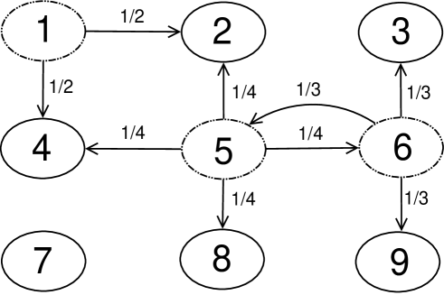
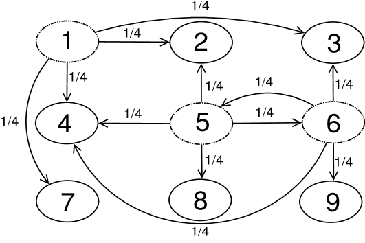
Figure 3.1 shows the transition probabilities for the firstly named application. Inside of the exploration area there is an equal probability of for flying forward, backward, to the left or right on a symmetric random walk. On the brinks of the area three directions remain and in the corners only two flight directions are still possible, at least when borders exist which should be standard case. Without borders the drones can leave the grid, only to reappear on the opposite side (see figure 3.2). In this case the transition probabilities remain at even for the marginal and corner states. For example, we present the transition matrix of the bordered symmetric random walk in table 2, whereupon entries with probability are omitted on grounds of clarity.
3.2. Calculation of the Expected Coverage
It takes some definitions concerning random variables to calculate the expected coverage of the symmetric random walk . Let indicate, if drone has visited state until point in time , thus whether a coverage occurred () or not. So, it is essential that
| (3.1) |
These random variables are Bernoulli-distributed with for now unknown parameters . It should be mentioned that for a constant point in time the random variables for neither are stochastically independent nor identical distributed which can be proven trivially. The same proposition can be made for all , if a particular state is considered. We will now confirm the dependence of the random variables in the last named case. But primarily, some characteristics of probability theory are needed.
Definition 3.1.
Independence of Events
Let be events at the same probability space. The events are stochastically independent if and only if for all and every index space of the cardinality
| (3.2) |
is valid.
Corollary 3.2.
Independence of Events
The events and are stochastically independent, if and only if or the equation
| (3.3) |
is satisfied for .
Proposition 3.3.
State Probabilities of a Markov Chain
The starting distribution is a - dimensional row vector and contains the probabilities for starting in each of the states . The state probabilities after time steps are calculated by
Below we proof the mentioned claim, which is the central conclusion of this paper.
Proposition 3.4.
Dependence of Coverage Events (1)
The events are stochastically dependent for and at least one state .
Proof.
The exploration area of the UAVs shall be big enough on grounds of realistic scenarios which requires a minimum cell count of five in each dimension. Apparently, the Markov chain holds for every point in time and state, because the drones keep in motion.
Case 1: The starting distribution has at least two states with an uneven Manhattan-distance to each other, that both have a positive probability on point in time zero.
In this case all states have a positive probability from a particular point in time onwards. Mathematically expressed, and apply from a particular point in time for every state . In worst-case, constitutes still less than width + depth for the two-dimensional case respectively width + depth + height for the three-dimensional case. The worst-case occurs, if the UAVs can only start from a corner, however state is located in the opposite corner. Not later than at this particular time applies
whereby the chronologically succeeding events and are stochastically dependent, likewise all chronologically succeeding events for arbitrary .
A typical special case of the first case is the starting distribution with an equal probability for every state. One realizes easily that the requirement in first case is achieved, if a random walk without borders has at least an uneven width, depth or height.
Case 2: The starting distribution has no pair of states with an uneven Manhattan-distance to each other.
A typical example is, if the drone takes off definitely from one particular whereabouts. It needs at the most width + depth (+ height) time steps, until approximately half of the states receive a positive probability. (If is even, there are exactly such states for the two-dimensional case; if is uneven, the number of such states switches between and ). Let this point in time be notated as . Now we pick a state and check the independence property as mentioned in corollary 3.2. The conditional probability is only defined, if is greater than zero. Otherwise the events and would be stochastically independent, which is true for up to half of the states in the bordered random walk for the second case. Below we will show that both events are even independent under the constraint .
| (3.4) | |||||
| (3.5) | |||||
| (3.6) | |||||
| (3.7) |
Hence it can be reasoned that both events are independent, if . This applies in the mentioned special case, if the drone departs definitely from one particular state. Then , and are independent for all states . On the contrary, for different starting distributions, and can be stochastically dependent, because at least two distinct states and provide the inequality .
To summarize, the events and are dependent if and only if
| (3.8) |
and
| (3.9) |
This should be valid in most examined Markov models at least for one state and . Below, the second case is analysed in more detail, in order to proof the dependence for some sub cases. Note that for the missing sub cases the dependence characteristic can be confirmed by checking the correctness of the above mentioned formulas 3.8 and 3.9, as soon as the concrete Markov model is created.
Special Case of case 2: Bordered Random Walk
We will focus on the two-dimensional bordered random walk, firstly with an uneven width and depth. The three-dimensional case proceeds similarly. The starting distribution shall be symmetric for now, for example the drone starts certainly in the middle of the grid. Let the point of time be such that in the corners , , and the states have a positive probability. Notice that this is only possible with an uneven width and depth. For the transition probability in two steps one can easily deduce . The unconditional probability can be obtained by formula
| (3.10) |
This implicates for the top left corner the equality
as a necessary and sufficient constraint for the independence. Due to the symmetric starting distribution all corner states provide the same probability whose sum can be at most . The outcome of this is which is less than , hence the condition 3.5 is not pervaded and therefore the events are dependent.
In some settings the starting distribution cannot be modelled as symmetric and the recent proof cannot be executed in an analogous manner, although the probabilities for the corner states will converge to the same positive value, if only even respectively uneven points in time are considered. Below we will consider not only an asymmetric starting distribution, but also a grid with at least one even dimension. At least half of the states have a positive probability on time step , if at least one corner state provides a positive probability. Remember that this is only true for times , , and so on in the event of uneven width and depth, but true for all times , , and so on in the event of at least one even dimension.
According to this, the average state probability of those states with a positive probability is not exceeding . It should be clear that the corner states provide a probability less than this in the long run because of the secluded location. So, for a particular corner state the probability should be . In grids of not less than states the probability becomes less than and therefore independence becomes impossible. The two-step probability remains at , but in big exploration areas each state is visited infrequently and the probability for being in a corner state drops below .
Case 3: Boundless Random Walk
A boundless random walk enables the UAVs to leave the grid on one side, in order to reappear on the other side. We will now examine a grid with at least one uneven dimension. A drone can fly in one direction and straight back in two time units. In a bordered random walk the recurrence time to any state is always even, in contrast in a boundless random walk with at least one uneven dimension a drone can back to the starting point in an uneven number of time steps, too. This reduces to the first case, by what the events are dependent. ∎
The objective is to calculate the expected coverage and therefore it is not in someone’s interest to have independent events but to have independent events and so on.
Claim 3.5.
The events and are independent, if and only if the complementary events and are independent.
Proof.
As argued before, the events and are independent, if and only if is valid.
The equation is true, if and only if is valid.∎
Theorem 3.6.
Dependence of Coverage Events (2)
The events are stochastically dependent for and at least one state .
It was shown that the considered events are stochastically dependent generally. Recall the definition
for the coverage of state up to time step . If one takes no notice of the dependence characteristic and assumes independence, the coverage probability of a single state is easy to calculate. The just made assumption leads to the coverage probability
| (3.11) |
like written in [1]. However, this formula cannot be true in general, because it disregards the presence of theorem 3.6. In order to take the dependence characteristic into account, one must specify appropriate Markov chains. Let the first arrival time in state be with the relation
State is visited until time , if and only if the first arrival in this state is at the latest on point of time. By reason of
| (3.12) |
the coverage probabilities can be reduced to the calculation of arrival probabilities. In order to receive the sought-after probabilities, we need to create a new Markov chain for every state in the considered random walk model. Subject to state the associated Markov chain is named . The just introduced new Markov chains accord with the Markov chain (for example as in table 2) nearly complete, but there are minor differences. State space and starting distribution coincide perfectly, but there is a change in row of the transition matrix . The transition matrix contains a one in row and column and zeros elsewhere in row , as is evident in table 3.
This change effects an altered behaviour of the Markov chain compared to . State is called absorbing, because the stochastic process remains in this state as soon as it has visited this state for the first time. Until this event, the behaviour of Markov chain is identical to that of the original Markov chain . In order to calculate the probability in the original Markov chain , we can go over to the new Markov chain which will be used henceforward. The first arrival time does not change, because both Markov chains behave exactly identical till the first arrival. In the new Markov model it meets to check the location of the random walk on point of time, because
| (3.13) |
holds. The probability of the latter term can be obtained, as customary in Markov chains, by multiplication of the starting distribution with the exponentiated transition matrix, thus
| (3.14) |
and the -th value of this row vector is selected. This can be done for all states , but remember that every state requires its own transition matrix . The expected coverage of the random walk after time steps is the expected value
| (3.15) |
divided by the number of states in the Markov model. It is about the ratio of the states in the Markov chain that has been visited after time steps, that is to be expected. Altogether the handling with dependent events leads to a much more complicated solution of the expected coverage as though one ignores this pre-assumption.
3.3. Independent Mobility
So far, the expected coverage of a single UAV was calculated. However, one of the greatest advantages of the operation of UAVs in contrary to helicopters is that the former can be used in groups, even at places with little room. Together they can explore the target area faster, especially if they cooperate. For the sake of convenience we limit on independent mobility, so that each drone uses the same Markov model for exploring, independent of the movement of the other UAVs. Thereby the coverage probability in 3.14 changes to
| (3.16) |
3.4. Comparison of Analytic and Simulation Results
The analytic solution of the expected coverage was deduced on the whole. The analytic results are confirmed by MCMC simulations which can be easily coded once the transition probabilities are available. However, there is a great gap between the analytic formula 3.11, that ignores the dependence of events, and the correct analytic results 3.14 as well as the simulation results. In [1] it is concluded that this peculiarity is due to error propagation. This argument can be excluded, because the correct formula 3.14 and the simulation results show no deviation and therefore are in agreement. On grounds of numerical computability, MCMC- simulations should be preferred opposite to the analytic formula, because the simulations can provide approximately exact results and can handle Markov models with huge state spaces considerably better.
4. Conclusions
In this work, we introduced Markov chains with and without borders in two and three dimensions. We deduced an analytic solution of the expected coverage in case of independent mobility. Though it was proven that certain events are not independent, which complicates the calculation vastly. The non-consideration of this fact leads to an incorrect solution for the expected coverage which cannot be explained by numerical inaccuracy. Hence, MCMC simulations provide still a good approximation for the analytic results.
References
- [1] E. Yanmaz, C. Costanzo, C. Bettstetter and W. Elmenreich, "A discrete stochastic process for coverage analysis of autonomous UAV networks," 2010 IEEE Globecom Workshops, Miami, FL, 2010, pp. 1777-1782.
- [2] Pierre Bremaud: Markov Chains: Gibbs Fields, Monte Carlo Simulation, and Queues. Berlin Heidelberg: Springer Science & Business Media, 2013.
- [3] R Core Team (2016). R: A language and environment for statistical computing. R Foundation for Statistical Computing, Vienna, Austria. URL https://www.R-project.org/.
Appendix: Sequencing in Three-Dimensional Grids
The sequencing and computation of the transition matrix for the bordered symmetric random walk in three-dimensional grids are programmed in R [3].