Witnessing quantum capacities of correlated channels

Abstract

We test a general method to detect lower bounds of the quantum channel capacity for two-qubit correlated channels. We consider in particular correlated dephasing, depolarising and amplitude damping channels. We show that the method is easily implementable, it does not require a priori knowledge about the channels, and it is very efficient, since it does not rely on full quantum process tomography.

I Introduction

The property of a quantum communication channel to convey quantum information is quantified in terms of the quantum capacity $Q$ lloyd ; barnum ; devetak ; hay , which corresponds to the maximum number of qubits that can be reliably transmitted per channel use. In any realistic scenario noise is unavoidably present and the amount of information that can be transmitted is lower than in the ideal noiseless case. It is therefore important to develop efficient means to establish whether the channel can still be profitably employed for information transmission in the presence of noise, that may be completely unknown.

A standard method to infer the effect of noise on a communication channel relies on quantum process tomography proc , but this, however, is a demanding procedure in terms of the number of different measurement settings needed, since it scales as $d^{4}$ for a finite $d$-dimensional quantum system. In Ref. ourl a method was recently proposed to gain some information on the channel ability to transmit quantum information by employing a smaller number of measurements, that scales as $d^{2}$. A lower bound on the quantum channel capacity was derived and it was shown that it can be experimentally accessed with a simple procedure. Such a procedure can be applied to any unknown quantum communication channel. The efficiency of the method was tested for many examples of single qubit channels, and for the generalised Pauli channel in arbitrary finite dimension.

In this paper we generalise this detection method to correlated qubit channels and test its efficiency in this case. Correlated qubit channels were originally studied in terms of classical information transmission and it was shown that for certain ranges of the correlation strengths the use of entanglement allows one to enhance the amount of transmitted information along the channel kn:2002-macchiavello-palma-pra . Quantum memory (or correlated) channels then attracted growing attention, and interesting new features emerged by modeling of relevant physical examples, including depolarizing channels MMM , Pauli channels mpv04 ; daems ; dc , dephasing channels hamada ; dbf ; ps ; gabriela ; lidar , amplitude damping channels vsdamp ; vs2 , Gaussian channels cerf , lossy bosonic channels mancini ; lupo , spin chains spins , collision models collision and a micro-maser model micromaser (for a recent review on quantum channels with memory effects see Ref. memo_review ).

The paper is organized as follows. In Sec. II we review the method of bounding the quantum capacity by means of the Shannon entropy pertaining to a vector of probabilities that can be inferred by performing few measurements on the output of the channel and a reference system. In the subsequent sections we apply the method to two-qubit correlated channels, considering explicitly the memory dephasing channel (Sec. III), the memory depolarizing channels (Sec. IV), and the fully correlated damping channel (Sec. V). We summarise the results of the paper in Sec. VI.

II Detection method

Let us consider a generic quantum channel ${\cal E}$ acting on a single system, and define ${\cal E}_{N}={\cal E}^{\otimes N}$, where $N$ represents the number of channel uses. The quantum capacity $Q$ is defined as lloyd ; barnum ; devetak ; hay

$$Q=\lim_{N\to\infty}\frac{Q_{N}}{N}\;,$$ (1)

where $Q_{N}=\max_{\rho}I_{c}(\rho,{\cal E}_{N})$, and $I_{c}(\rho,{\cal E}_{N})$ denotes the coherent information schumachernielsen

$$I_{c}(\rho,{\cal E}_{N})=S[{\cal E}_{N}(\rho)]-S_{e}(\rho,{\cal E}_{N})\;.$$ (2)

In Eq. (2), $S(\rho)=-\operatorname{Tr}[\rho\log_{2}\rho]$ is the von Neumann entropy, and $S_{e}(\rho,{\cal E})$ represents the entropy exchange schumacher , i.e. $S_{e}(\rho,{\cal E})=S[({\cal I}_{R}\otimes{\cal E})(|\Psi_{\rho}\rangle\langle\Psi_{\rho}|)]$, where $|\Psi_{\rho}\rangle$ is any purification of $\rho$ by means of a reference quantum system $R$, namely $\rho=\operatorname{Tr}_{R}[|\Psi_{\rho}\rangle\langle\Psi_{\rho}|]$.

In Ref. ourl we derived a lower bound for the quantum capacity $Q$ that can be easily accessed without requiring full process tomography of the quantum channel. We briefly review the derivation here in the following. For any complete set of orthogonal projectors $\{\Pi_{i}\}$, one has NC00 $S(\rho)\leq S(\sum_{i}\Pi_{i}\rho\Pi_{i})$. Then, for any orthonormal basis $\{|\Phi_{i}\rangle\}$ for the tensor product of the reference and the system Hilbert spaces, one has the following bound to the entropy exchange

$$S_{e}\left(\rho,{\cal E}\right)\leq H(\vec{p})\;,$$ (3)

where $H(\vec{p})\equiv-\sum_{i}p_{i}\log_{2}p_{i}$ denotes the Shannon entropy for the vector of the probabilities $\{p_{i}\}$, with

$$p_{i}=\operatorname{Tr}[({\cal I}_{R}\otimes{\cal E})(|\Psi_{\rho}\rangle\langle\Psi_{\rho}|)|\Phi_{i}\rangle\langle\Phi_{i}|]\;.$$ (4)

From Eq. (3) one obtains the following chain of bounds

$$Q\geq Q_{1}\geq I_{c}(\rho,{\cal E}_{1})\geq S\left[{\cal E}(\rho)\right]-H(\vec{p})\equiv Q_{DET}\;,$$ (5)

which holds for any $\rho$ and $\vec{p}$. A lower bound $Q_{DET}$ to the quantum capacity of an unknown channel can then be detected by preparing a bipartite pure state $|\Psi_{\rho}\rangle$ and sending it through the channel ${\cal I}_{R}\otimes{\cal E}$, where the unknown channel ${\cal E}$ acts on one of the two subsystems. Suitable local observables on the joint output state are then measured in order to estimate $S\left[{\cal E}(\rho)\right]$ and $\vec{p}$, and to compute $Q_{DET}$. Typically, for a fixed measurement setting, one can infer different vectors of probabilities pertaining to different sets of orthogonal projectors, as will be shown in the following. Moreover, one could also adopt an adaptive detection scheme to improve the bound (5) by varying the input state $|\Psi_{\rho}\rangle$. Since no information is given a priori about the communication channel, typically we always choose a maximally entangled input state, so that the reduced input $\rho$ has maximum input entropy.

We will assume that only the local observables $O_{i}\otimes O_{i}$ on the system and reference are measured, where $\{O_{i}\}$ is a tomographically complete set on the system alone. Notice that the above measurements allow one to measure $\{O_{i}\}$ on the system alone by ignoring the statistics of the measurement results on the reference. In this way, a complete tomography of the system output state can be performed, and therefore the term $S\left[{\cal E}(\rho)\right]$ in Eq. (5) can be estimated exactly. Our goal is to optimize the bound $Q_{DET}$ given these resources. This procedure requires $d^{2}-1$ measurement settings with respect to a complete process tomography, where $d^{4}-1$ observables have to be measured: this choice greatly simplifies the experimental setup to detect the quantum capacity.

Let us now consider explicitly the case of qubits with $\{O_{i}\}=\{\sigma_{x},\sigma_{y},\sigma_{z}\}$. By denoting the Bell states as

$$\!\!\!\!\!|\Phi^{\pm}\rangle=\frac{1}{\sqrt{2}}(|00\rangle\pm|11\rangle)\,,\ \ |\Psi^{\pm}\rangle=\frac{1}{\sqrt{2}}(|01\rangle\pm|10\rangle)\,,$$ (6)

it can be proven ourl that the local measurement settings $\{\sigma_{x}\otimes\sigma_{x},\sigma_{y}\otimes\sigma_{y},\sigma_{z}\otimes\sigma_{z}\}$ allow one to estimate the vector $\vec{p}$ pertaining to the projectors onto the following inequivalent bases

$$B_{1}= \{a|\Phi^{+}\rangle+b|\Phi^{-}\rangle,-b|\Phi^{+}\rangle+a|\Phi^{-}\rangle,$$ (7)

$$\ c|\Psi^{+}\rangle+d|\Psi^{-}\rangle,-d|\Psi^{+}\rangle+c|\Psi^{-}\rangle\}\;,$$

$$B_{2}= \{a|\Phi^{+}\rangle+b|\Psi^{+}\rangle,-b|\Phi^{+}\rangle+a|\Psi^{+}\rangle,$$ (8)

$$c|\Phi^{-}\rangle+d|\Psi^{-}\rangle,-d|\Phi^{-}\rangle+c|\Psi^{-}\rangle\}\;,$$

$$B_{3}= \{a|\Phi^{+}\rangle+ib|\Psi^{-}\rangle,ib|\Phi^{+}\rangle+a|\Psi^{-}\rangle,$$ (9)

$$c|\Phi^{-}\rangle+id|\Psi^{+}\rangle,id|\Phi^{-}\rangle+c|\Psi^{+}\rangle\}\;,$$

with $a,b,c,d$ real and such that $a^{2}+b^{2}=c^{2}+d^{2}=1$.

The probability vector $\vec{p}$ for each choice of basis is evaluated according to Eq. (4). In order to obtain the tightest bound in (5) given the fixed local measurements $\{\sigma_{x}\otimes\sigma_{x},\sigma_{y}\otimes\sigma_{y},\sigma_{z}\otimes\sigma_{z}\}$, the Shannon entropy $H(\vec{p})$ will be then minimised as a function of the bases (7-9), by varying the coefficients $a,b,c,d$ over the three sets. In an experimental scenario, after collecting the outcomes of the measurements $\{\sigma_{x}\otimes\sigma_{x},\sigma_{y}\otimes\sigma_{y},\sigma_{z}\otimes\sigma_{z}\}$, this optimisation step corresponds to classical processing of the measurement outcomes.

The simplification of choosing a restricted set of measurements may generally come at a cost, since the evaluated Shannon entropy $H(\vec{p})$ in Eq. (5) may give a poor bound to the quantum capacity. Even for a unitary transformation a simplified measurement setting could be inefficient to provide a detectable bound. For example, a detection scheme for qubits for the unitary channels

$$U=\frac{1}{2}\left(I+i\sum_{\alpha=x,y,z}\epsilon_{\alpha}\sigma_{\alpha}\right)\;,\qquad\epsilon_{\alpha}=\pm 1\;,$$ (10)

with input $|\Phi^{+}\rangle$ and measurement on any of the bases (6–9) gives always a uniform probability vector, hence $H(\vec{p})=2$. In these cases it is mandatory to adopt an adaptive detection scheme: clearly, by varying the input state to $(I_{R}\otimes U^{\dagger})|\Phi^{+}\rangle$ one obtains $H(\vec{p})=0$ from the Bell basis (6), thus recovering the result $Q_{DET}=1$. A further possibility is to support our method with efficient estimation methods for unitaries Koch .

We remember that the bound we are providing also gives detectable lower bounds to the private information devetak ; ourl and the entanglement-assisted classical capacity thapliyal ; hol2 ; ourl .

III Correlated dephasing channel

We consider a dephasing quantum channel that maps two-qubit input states $\rho$ onto

$$\mathcal{E}(\rho)=\sum_{i_{1},i_{2}}A_{i_{1},i_{2}}\rho A^{\dagger}_{i_{1},i_{2}},\quad\quad i_{k}=0,1,$$ (11)

where Kraus operators $A_{i_{1},i_{2}}$ are defined in terms of the Pauli operators $\sigma_{0}=I$ and $\sigma_{1}=\sigma_{z}$ as follows

$$A_{i_{1},i_{2}}=\sqrt{p_{i_{1},i_{2}}}B_{i_{1},i_{2}},\quad B_{i_{1},i_{2}}\equiv\sigma_{i_{1}}^{(1)}\otimes\sigma_{i_{2}}^{(2)},$$ (12)

with $\sum_{\{i_{k}\}}p_{i_{1},i_{2}}=1$, and $\sigma_{i_{k}}^{(k)}$ acting on the $k$-th qubit.

We describe the joint probabilities in Eq. (12) by a Markov chain kn:2002-macchiavello-palma-pra ; hamada , namely

$$p_{i_{1},i_{2}}=p_{i_{1}}p_{i_{2}|i_{1}},$$ (13)

with

$$p_{i_{2}|i_{1}}=(1-\mu)\,p_{i_{2}}+\mu\,\delta_{i_{1},i_{2}}.$$ (14)

The parameter $\mu\in[0,1]$ measures degree of correlation of the channel: it is the probability that the same operator (either $I$ or $\sigma_{z}$) is applied for two consecutive uses of the channel, whereas $1-\mu$ is the probability that the two operators are uncorrelated. The limiting cases $\mu=0$ and $\mu=1$ correspond to memoryless channels and channels with perfect memory, respectively. The correlated dephasing channel is easily shown to be degradable ds , hence $Q=Q_{1}$, and its quantum capacity is given by dbf ; ps ; physc

$$Q=\left\{2-p\,H_{2}[(1-p)(1-\mu)]-(1-p)\,H_{2}[p(1-\mu)]-H_{2}(p)\right\}\;,$$ (15)

where $p\equiv p_{1}$, and $H_{2}(p)\equiv-p\log_{2}p-(1-p)\log_{2}(1-p)$ denotes the binary Shannon entropy. Notice also that Eq. (15) is invariant by replacing $p$ with $(1-p)$.

We consider now a detection scheme with two input qubits $A$ and $B$ which are maximally entangled with two reference qubits $R_{A}$ and $R_{B}$, namely a global input state $|{\Phi^{+}}\rangle_{R_{A},A}|{\Phi^{+}}\rangle_{R_{B},B}$. The corresponding output state is given by

$$\Xi = {\cal I}_{R_{A}}\otimes{\cal I}_{R_{B}}\otimes{\cal E}_{2}(|{\Phi^{+}}\rangle\langle{\Phi^{+}}|_{R_{A},A}\otimes|{\Phi^{+}}\rangle\langle{\Phi^{+}}|_{R_{B},B})$$ (16)

$$= (1-p)[(1-p)(1-\mu)+\mu]|{\Phi^{+}}\rangle\langle{\Phi^{+}}|_{R_{A},A}\otimes|{\Phi^{+}}\rangle\langle{\Phi^{+}}|_{R_{B},B}$$

$$+ p[p(1-\mu)+\mu]|{\Phi^{-}}\rangle\langle{\Phi^{-}}|_{R_{A},A}\otimes|{\Phi^{-}}\rangle\langle{\Phi^{-}}|_{R_{B},B}$$

$$+ p(1-p)(1-\mu)|{\Phi^{+}}\rangle\langle{\Phi^{+}}|_{R_{A},A}\otimes|{\Phi^{-}}\rangle\langle{\Phi^{-}}|_{R_{B},B}$$

$$+ p(1-p)(1-\mu)|{\Phi^{-}}\rangle\langle{\Phi^{-}}|_{R_{A},A}\otimes|{\Phi^{+}}\rangle\langle{\Phi^{+}}|_{R_{B},B}\;.$$

The reduced input state for qubits $A$ and $B$ is simply $\frac{1}{4}I_{A}\otimes I_{B}$, and it remains invariant under the action of ${\cal E}$, hence the reduced output entropy equals 2 bits. We consider a measurement scheme on the output state (16) where the set of observables $\sigma_{x}\otimes\sigma_{x}$, $\sigma_{y}\otimes\sigma_{y}$, and $\sigma_{z}\otimes\sigma_{z}$ are measured on both couples of qubits $R_{A},A$ and $R_{B},B$. Such a scheme provides the vector of probabilities

$$\vec{p}=\{(1-p)[(1-p)(1-\mu)+\mu],p[p(1-\mu)+\mu],p(1-p)(1-\mu),p(1-p)(1-\mu)\}\;.$$ (17)

A straightforward calculation shows that the detected quantum capacity coincides with the quantum capacity, namely

$$Q\equiv Q_{DET}=2-H(\vec{p})\;.$$ (18)

Our detected bound provides exactly the quantum capacity, since $Q=Q_{1}$ due to the degradability of the channel, and the components of the vector $\vec{p}$ in Eq. (17) correspond to the eigenvalues of the joint output state (16). In Fig. (1) we plot the detected capacity (15) versus the correlation parameter $\mu$, for the following values $p=0.01,\ 0.1,\ 0.2,\ 0.3,\ 0.5$ (or, equivalently, $p=0.99,\ 0.9,\ 0.8,\ 0.7,\ 0.5$).

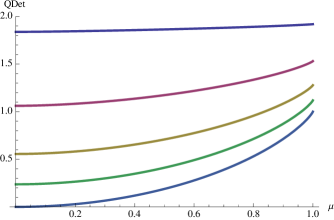
Figure 1: Detected quantum capacity for the correlated dephasing channel versus the correlation parameter $\mu$ for different values of the probability $p$ (from top to bottom $p=0.01,\ 0.1,\ 0.2,\ 0.3,\ 0.5$). Two maximally entangled input states are used and Bell measurements are considered. The curves coincide with the quantum capacity given by Eq. (15).

IV Correlated depolarizing channel

We study the following correlated depolarizing quantum channel kn:2002-macchiavello-palma-pra that maps two-qubit input states $\rho$ onto

$$\mathcal{E}(\rho)=\sum_{i_{1},i_{2}}A_{i_{1},i_{2}}\rho A^{\dagger}_{i_{1},i_{2}},\quad\quad i_{k}=0,1,2,3$$ (19)

where Kraus operators are defined as in Eq. (12), now with $\sigma_{0}=I\,,\ \sigma_{1}=\sigma_{z}\,,\ \sigma_{2}=\sigma_{x}\,,\ \sigma_{3}=\sigma_{y}$. The joint probabilities still satisfy the Markov chain rule as in Eqs. (13,14), with $p_{0}=1-p$ and $p_{1}=p_{2}=p_{3}=\frac{p}{3}$.

As in the previous case, the parameter $\mu\in[0,1]$ measures the degree of correlation of the channel: it is the probability that the same operator $\sigma_{i}$ is applied for two consecutive uses of the channel, whereas $1-\mu$ is the probability that the two operators are uncorrelated. Again, the limiting cases $\mu=0$ and $\mu=1$ correspond to memoryless channels and channels with perfect correlation, respectively.

Let us consider now two input qubits $A$ and $B$ which are maximally entangled with two reference qubits $R_{A}$ and $R_{B}$, namely an input $|{\Phi^{+}}\rangle_{R_{A},A}|{\Phi^{+}}\rangle_{R_{B},B}$. We also rename the Bell states as follows

$$|{\Phi_{0}}\rangle\equiv|{\Phi^{+}}\rangle\;,$$

$$|{\Phi_{1}}\rangle\equiv|{\Phi^{-}}\rangle\;,$$

$$|{\Phi_{2}}\rangle\equiv|{\Psi^{+}}\rangle\;,$$

$$|{\Phi_{3}}\rangle\equiv|{\Psi^{-}}\rangle\;.$$ (20)

The output state can then be written as

$$\Xi = {\cal I}_{R_{A}}\otimes{\cal I}_{R_{B}}\otimes{\cal E}(|{\Phi_{0}}\rangle\langle{\Phi_{0}}|_{R_{A},A}\otimes|{\Phi_{0}}\rangle\langle{\Phi_{0}}|_{R_{B},B})$$ (21)

$$= \sum_{i,j=0}^{3}p_{ij}|{\Phi_{i}}\rangle\langle{\Phi_{i}}|_{R_{A},A}\otimes|{\Phi_{j}}\rangle\langle{\Phi_{j}}|_{R_{B},B}\;,$$

where

$$p_{00}=(1-\mu)(1-p)^{2}+\mu(1-p)\,,$$

$$p_{ii}=(1-\mu)\left(\frac{p}{3}\right)^{2}+\mu\frac{p}{3}\,,\qquad i=1,2,3\,,$$

$$p_{ij}=(1-\mu)\left(\frac{p}{3}\right)^{2}\,,\qquad i,j=1,2,3\quad i\neq j\,,$$

$$p_{0i}=p_{i0}=(1-\mu)\frac{p}{3}(1-p)\,,\qquad i=1,2,3\;.$$ (22)

The reduced input state is simply $\frac{1}{4}I_{A}\otimes I_{B}$, and remains invariant under the action of ${\cal E}$, hence the reduced output entropy equals 2 bits. A measurement scheme on the output state (21) where the set of observables $\sigma_{x}\otimes\sigma_{x}$, $\sigma_{y}\otimes\sigma_{y}$, and $\sigma_{z}\otimes\sigma_{z}$ are measured on both couples of qubits $R_{A},A$ and $R_{B},B$ provides all probabilities $p_{ij}$ in Eq. (22).

Then, we can write our detected bound as follows

$$Q\geq Q_{DET}=[2-H(\{p_{ij}\})]=2+p_{00}\log_{2}p_{00}+3p_{11}\log_{2}p_{11}+6p_{12}\log_{2}p_{12}+6p_{01}\log_{2}p_{01}\;.$$ (23)

The detected capacity $Q_{DET}$ coincides with the maximum of the coherent information evaluated in Ref. physc for a single use of the memory channel (19). Since the channel is not degradable, $Q_{DET}$ is just a lower bound of the quantum channel capacity, whose exact expression is still unknown.

We notice, however, that for the fully correlated channel, i.e. $\mu=1$, Kraus operators $\{\sigma_{i}\otimes\sigma_{i}\}$ are a commuting set, hence the channel is degradable ds and one has

$$Q\equiv Q_{DET}=Q=2-H_{2}(p)-p\log_{2}3\;,$$ (24)

which corresponds to the exact quantum capacity, that is therefore efficiently detected by our method. The result of Eq. (24) can be easily generalized to the case of fully correlated depolarized channels for qudits, thus giving

$$Q\equiv Q_{DET}=Q=d-H_{2}(p)-p\log_{2}(d^{2}-1)\;.$$ (25)

In Fig. (2) we plot the detected bound (23) versus the correlation parameter $\mu$, for the following values $p=0.005,\ 0.05,\ 0.1,\ 0.15,\ 0.2$.

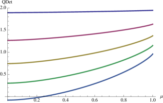
Figure 2: Detected quantum capacity for the correlated depolarizing channel versus memory parameter $\mu$ for different values of the probability $p$ (from top to bottom $p=0.005,\ 0.05,\ 0.1,\ 0.15,\ 0.2$). The detected quantum capacity is given by Eq. (23) using two maximally entangled input states and Bell measurement.

V Fully correlated damping channel

In this section we consider the following correlated amplitude damping channel acting on two qubits vsdamp

$${\cal E}(\rho)=\sum_{i=1}^{2}B_{i}\,\rho\,B_{i}^{\dagger},$$ (26)

with Kraus operators

$${B}_{1}=\left(\begin{array}[]{cccc}1&0&0&0\\ 0&1&0&0\\ 0&0&1&0\\ 0&0&0&\sqrt{\eta}\\ \end{array}\right),\,\,\qquad{B}_{2}=\left(\begin{array}[]{cccc}0&0&0&\sqrt{1-\eta}\\ 0&0&0&0\\ 0&0&0&0\\ 0&0&0&0\\ \end{array}\right),$$ (27)

where the ordered basis $\{|{00}\rangle,|{01}\rangle,|{10}\rangle,|{11}\rangle\}$ has been used. This channel describes a fully correlated damping, namely only the state $|{11}\rangle$ undergoes decay to $|{00}\rangle$ with probability $\eta$, while the other states $|{00}\rangle,|{01}\rangle,|{10}\rangle$ remain unaltered.

We only consider the fully correlated case, because for partially correlated amplitude damping channels just numerical bounds on the quantum capacity are known vs2 . On the other hand, the fully correlated amplitude damping channel has been shown to be degradable for $\eta\geq 1/2$, and its quantum capacity is explicitly obtained by the following maximization vsdamp

$$Q = \max_{\alpha,\beta,\delta}\Big{\{}-[\alpha+(1-\eta)\delta]\log_{2}[\alpha+(1-\eta)\delta]-2\beta\log_{2}\beta\,-\,\eta\delta\log_{2}\eta\delta\,+\,$$ (28)

$$+[1-(1-\eta)\delta]\log_{2}[1-(1-\eta)\delta]+\,(1-\eta)\delta\log_{2}[(1-\eta)\delta]\Big{\}},$$

with the constraints $\alpha+2\beta+\delta=1$ and $\alpha,\beta,\delta\geq 0$. For $\eta\leq 1/2$, one simply has $Q=\log_{2}3$, corresponding just to coding on the noiseless subspace spanned by $\{|{00}\rangle,|{01}\rangle,|{10}\rangle\}$.

As in the previous examples, we consider an input maximally entangled state between the two qubits $A$ and $B$ with two reference qubits $R_{A}$ and $R_{B}$, namely $|{\Phi^{+}}\rangle_{R_{A},A}|{\Phi^{+}}\rangle_{R_{B},B}$. The output state is then given by

$$\Xi={\cal I}_{R_{A}}\otimes{\cal I}_{R_{B}}\otimes{\cal E}(|{\Phi^{+}}\rangle\langle{\Phi^{+}}|_{R_{A},A}\otimes|{\Phi^{+}}\rangle\langle{\Phi^{+}}|_{R_{B},B})\;.$$ (29)

Notice that Kraus operators $B_{1}$ and $B_{2}$ in Eq. (27) can be rewritten as

$$B_{1}=\frac{3+\sqrt{\eta}}{4}I_{A}\otimes I_{B}+\frac{1-\sqrt{\eta}}{4}\sigma_{zA}\otimes I_{B}+\frac{1-\sqrt{\eta}}{4}I_{A}\otimes\sigma_{zB}-\frac{1-\sqrt{\eta}}{4}\sigma_{zA}\otimes\sigma_{zB}\;$$

$$B_{2}=\frac{\sqrt{1-\eta}}{4}(\sigma_{xA}+i\sigma_{yA})\otimes(\sigma_{xB}+i\sigma_{yB})\;.$$ (30)

It follows that the output state (29) has a block-diagonal form, i.e. $\Xi=\Xi_{1}\oplus\Xi_{2}$, with

$$\Xi_{1} = B_{1}(|{\Phi^{+}}\rangle\langle{\Phi^{+}}|_{R_{A},A}\otimes|{\Phi^{+}}\rangle\langle{\Phi^{+}}|_{R_{B},B})B_{1}^{\dagger}$$ (35)

$$= y_{\eta}\left(\begin{array}[]{cccc}x_{\eta}^{2}&x_{\eta}&x_{\eta}&x_{\eta}\\ x_{\eta}&1&1&1\\ x_{\eta}&1&1&1\\ x_{\eta}&1&1&1\\ \end{array}\right)\;,$$

on the ordered basis $\{|{\Phi^{+}}\rangle_{R_{A},A}|{\Phi^{+}}\rangle_{R_{B},B},|{\Phi^{+}}\rangle_{R_{A},A}|{\Phi^{-}}\rangle_{R_{B},B},|{\Phi^{-}}\rangle_{R_{A},A}|{\Phi^{+}}\rangle_{R_{B},B},|{\Phi^{-}}\rangle_{R_{A},A}|{\Phi^{-}}\rangle_{R_{B},B}\}$, with

$$y_{\eta}=\frac{(1-\sqrt{\eta})^{2}}{16},\qquad x_{\eta}=\frac{3+\sqrt{\eta}}{1-\sqrt{\eta}}\;,$$ (36)

whereas

$$\Xi_{2}=B_{2}(|{\Phi^{+}}\rangle\langle{\Phi^{+}}|_{R_{A},A}\otimes|{\Phi^{+}}\rangle\langle{\Phi^{+}}|_{R_{B},B})B_{2}^{\dagger}=\frac{1-\eta}{4}{|{10}\rangle\langle{10}|}_{R_{A},A}\otimes{|{10}\rangle\langle{10}|}_{R_{B},B}\;.$$ (37)

The reduced output state is given by

$${\cal E}\left(\frac{I_{A}}{2}\otimes\frac{I_{B}}{2}\right)=\frac{1}{4}\left(\begin{array}[]{cccc}2-\eta&0&0&0\\ 0&1&0&0\\ 0&0&1&0\\ 0&0&0&\eta\\ \end{array}\right)\,,$$ (42)

on the ordered basis $\{|{00}\rangle,|{01}\rangle,|{10}\rangle,|{11}\rangle\}$. Notice that the present channel is clearly an example of non-unital channel.

We consider now a detection scheme on the output state where the set of observables $\sigma_{x}\otimes\sigma_{x}$, $\sigma_{y}\otimes\sigma_{y}$, and $\sigma_{z}\otimes\sigma_{z}$ are measured on both couples of qubits $R_{A},A$ and $R_{B},B$. The set of probabilities that can be obtained by this measurement setting and minimizes the Shannon entropy $H(\vec{p})$, corresponds to the set of projectors on the following states

$${|{00}\rangle}_{R_{A},A}{|{01}\rangle}_{R_{B},B}\;,{|{00}\rangle}_{R_{A},A}{|{10}\rangle}_{R_{B},B}\;,{|{11}\rangle}_{R_{A},A}{|{01}\rangle}_{R_{B},B}\;,{|{11}\rangle}_{R_{A},A}{|{10}\rangle}_{R_{B},B}\;,$$

$${|{01}\rangle}_{R_{A},A}{|{00}\rangle}_{R_{B},B}\;,{|{01}\rangle}_{R_{A},A}{|{01}\rangle}_{R_{B},B}\;,{|{01}\rangle}_{R_{A},A}{|{10}\rangle}_{R_{B},B}\;,{|{01}\rangle}_{R_{A},A}{|{11}\rangle}_{R_{B},B}\;,$$

$${|{10}\rangle}_{R_{A},A}{|{00}\rangle}_{R_{B},B}\;,{|{10}\rangle}_{R_{A},A}{|{01}\rangle}_{R_{B},B}\;,{|{10}\rangle}_{R_{A},A}{|{11}\rangle}_{R_{B},B}\;,$$ (43)

for which $p=0$,

$${|{10}\rangle}_{R_{A},A}{|{10}\rangle}_{R_{B},B}\;,$$ (44)

for which $p=\frac{1-\eta}{4}$, and nota

$$|\chi_{1}\rangle\equiv(a{|{\Phi^{+}}\rangle}_{R_{A},A}+b{|{\Phi^{-}}\rangle}_{R_{A},A})(a{|{\Phi^{+}}\rangle}_{R_{B},B}+b{|{\Phi^{-}}\rangle}_{R_{B},B})\;,$$

$$|\chi_{2}\rangle\equiv(a{|{\Phi^{+}}\rangle}_{R_{A},A}+b{|{\Phi^{-}}\rangle}_{R_{A},A})(-b{|{\Phi^{+}}\rangle}_{R_{B},B}+a{|{\Phi^{-}}\rangle}_{R_{B},B})\;,$$

$$|\chi_{3}\rangle\equiv(-b{|{\Phi^{+}}\rangle}_{R_{A},A}+a{|{\Phi^{-}}\rangle}_{R_{A},A})(a{|{\Phi^{+}}\rangle}_{R_{B},B}+b{|{\Phi^{-}}\rangle}_{R_{B},B})\;,$$

$$|\chi_{4}\rangle\equiv(-b{|{\Phi^{+}}\rangle}_{R_{A},A}+a{|{\Phi^{-}}\rangle}_{R_{A},A})(-b{|{\Phi^{+}}\rangle}_{R_{B},B}+a{|{\Phi^{-}}\rangle}_{R_{B},B})\;,$$ (45)

with $a$ and $b$ real, such that $a^{2}+b^{2}=1$ and $-\sum_{i=1}^{4}q_{i}\log_{2}q_{i}$ is minimized, where

$$q_{i}=\langle\chi_{i}|\Xi_{1}|\chi_{i}\rangle\;.$$ (46)

We can now write the detection bound as follows

$$Q\geq Q_{DET}=H({\vec{s}}\,)-H_{2}\left(\frac{1-\eta}{4}\right)-H({\vec{q}}\,)\;,$$ (47)

where $\vec{s}=\{(2-\eta)/4,1/4,1/4,\eta/4\}$ corresponds to the eigenvalues of the output reduced state (42), and $\vec{q}=\{q_{1},q_{2},q_{3},q_{4}\}$.

In Fig. 3 we plot the detection bound along with the quantum capacity of the fully correlated amplitude damping channel versus damping parameter $\eta$. The looseness of the bound for $\eta<1/2$ is due to the fact the input maximally entangled state is very suboptimal for strong damping. Notice, however, that the positivity of the quantum capacity is witnessed for all values of $\eta$.

Figure 3: Fully correlated amplitude damping channel with parameter $\eta$: detected quantum capacity (thick line) with maximally entangled input and projective measurement on states (43,44,45), along with the theoretical quantum capacity (dashed line) given by Eq. (28).

VI Conclusions

We have applied a general method to witness lower bounds to the quantum capacity of quantum communication channels developed in Ref. ourl to the case of correlated qubit channels. We have shown that our method does not require any a priori knowledge about the channel itself and relies on a number of measurement settings that scales more favorably with respect to full process tomography. Specifically, we tested the method on two-qubit correlated channels of dephasing, depolarizing and amplitude damping type, and showed that a fixed maximally entangled input state of two system qubits and two reference qubits, and a setting of local measurements allow one to certify the quantum capacity, without the need of a complete tomographical reconstruction of the channel operation. We want to emphasize that for quantum optical systems our method is easily implementable with present-day technologies tech .

References

• (1) S. Lloyd, Phys. Rev. A 55, 1613 (1997).
• (2) H. Barnum, M. A. Nielsen, and B. Schumacher, Phys. Rev. A 57, 4153 (1998).
• (3) I. Devetak, IEEE Trans. Inf. Theory 51, 44 (2003).
• (4) P. Hayden, M. Horodecki, A. Winter, and J. Yard, Open Sys. Inf. Dyn. 15, 7 (2008).
• (5) I. L. Chuang and M. A. Nielsen, J. Mod. Opt. 44, 2455 (1997); J. F. Poyatos, J. I. Cirac, and P. Zoller, Phys. Rev. Lett. 78, 390 (1997); M. F. Sacchi, Phys. Rev. A 63, 054104 (2001); G. M. D’Ariano and P. Lo Presti, Phys. Rev. Lett. 86, 4195 (2001); M. Mohseni, A. T. Rezakhani, and D. A. Lidar, Phys. Rev. A 77, 032322 (2008).
• (6) C. Macchiavello and M. F. Sacchi, Phys. Rev. Lett. 116, 140501 (2016).
• (7) C. Macchiavello and G. M. Palma, Phys. Rev. A 65, 050301(R) (2002).
• (8) L. Memarzadeh, C. Macchiavello, and S. Mancini, New J. Phys. 13, 103031 (2011).
• (9) C. Macchiavello, G. M. Palma, and S. Virmani, Phys. Rev. A 69, 010303(R) (2004).
• (10) D. Daems, Phys. Rev. A 76, 012310 (2007).
• (11) Z. Shadman, H. Kampermann, D. Bruss, and C. Macchiavello, Phys. Rev. A 84, 042309 (2011); Z. Shadman, H. Kampermann, D. Bruss, and C. Macchiavello, Phys. Rev. A 85, 052306 (2012).
• (12) H. Hamada, J. Math. Phys. 43, 4382 (2002).
• (13) A. D’Arrigo, G. Benenti, and G. Falci, New J. Phys. 9, 310 (2007).
• (14) M. B. Plenio and S. Virmani, Phys. Rev. Lett. 99, 120504 (2007).
• (15) G. Barreto Lemos and G. Benenti, Phys. Rev. A 81, 062331 (2010).
• (16) N. Arshed, A. H. Toor, and D. A. Lidar, Phys. Rev. A 81, 062353 (2010).
• (17) A. D’Arrigo, G. Benenti, G. Falci, and C. Macchiavello, Phys. Rev. A 88, 042337 (2013).
• (18) A. D’Arrigo, G. Benenti, G. Falci, and C. Macchiavello, Phys. Rev. A 92, 062342 (2015).
• (19) N. J. Cerf, J. Clavareau, C. Macchiavello, and J. Roland, Phys. Rev. A 72, 042330 (2005).
• (20) O. V. Pilyavets, V. G. Zborovskii, and S. Mancini, Phys. Rev. A 77, 052324 (2008).
• (21) C. Lupo, V. Giovannetti, and S. Mancini, Phys. Rev. Lett. 104, 030501 (2010).
• (22) A. Bayat, D. Burgarth, S. Mancini, and S. Bose, Phys. Rev. A 77, 050306(R) (2008).
• (23) V. Giovannetti and G. M. Palma, Phys. Rev. Lett. 108, 040401 (2012).
• (24) G. Benenti, A. D’Arrigo, and G. Falci, Phys. Rev. Lett. 103, 020502 (2009); A. D’Arrigo, G. Benenti, and G. Falci, Eur. Phys. J. D 66, 147 (2012).
• (25) F. Caruso, V. Giovannetti, C. Lupo, and S. Mancini, Rev. Mod. Phys. 86, 1203 (2014).
• (26) B. W. Schumacher and M. A. Nielsen, Phys. Rev. A 54, 2629 (1996).
• (27) B. W. Schumacher, Phys. Rev. A 54, 2614 (1996).
• (28) I. L. Chuang and M. A. Nielsen, Quantum Information and Communication (Cambridge, Cambridge University Press, 2000).
• (29) D. M Reich, G. Gualdi, and C. Koch, Phys. Rev. Lett. 111, 200401 (2013).
• (30) C. H. Bennett, P. W. Shor, J. A. Smolin, and A. V. Thapliyal, Phys. Rev. Lett. 83, 3081 (1999).
• (31) A. S. Holevo, J. Math. Phys. 43, 4326 (2002).
• (32) I. Devetak and P. W. Shor, Commun. Math. Phys. 256, 287 (2005).
• (33) P. Huang, G. He, Y. Lu, and G. Zeng, Phys. Scr. 83, 015005 (2011).
• (34) For the subspace spanned by $\{|{\Phi^{+}}\rangle_{R_{A},A}|{\Phi^{+}}\rangle_{R_{B},B},|{\Phi^{+}}\rangle_{R_{A},A}|{\Phi^{-}}\rangle_{R_{B},B},|{\Phi^{-}}\rangle_{R_{A},A}|{\Phi^{+}}\rangle_{R_{B},B},|{\Phi^{-}}\rangle_{R_{A},A}|{\Phi^{-}}\rangle_{R_{B},B}\}$, the detection scheme where the set of observables $\sigma_{x}\otimes\sigma_{x}$, $\sigma_{y}\otimes\sigma_{y}$, and $\sigma_{z}\otimes\sigma_{z}$ are measured on both couples of qubits $R_{A},A$ and $R_{B},B$ allows one to generally estimate the probabilities pertaining to projectors on states of the form
$\displaystyle|\psi\rangle=A|{\Phi^{+}}\rangle_{R_{A},A}|{\Phi^{+}}\rangle_{R_{B},B}+B|{\Phi^{+}}\rangle_{R_{A},A}|{\Phi^{-}}\rangle_{R_{B},B}+C|{\Phi^{-}}\rangle_{R_{A},A}|{\Phi^{+}}\rangle_{R_{B},B}+D|{\Phi^{-}}\rangle_{R_{A},A}|{\Phi^{-}}\rangle_{R_{B},B}\;,$
with $A,B,C,D$ real, and satisfying $A^{2}+B^{2}+C^{2}+D^{2}=1$ along with $AD=BC$. This is equivalent to factorized states in the $A-B$ cut, namely
$\displaystyle|\psi\rangle\equiv(a{|{\Phi^{+}}\rangle}_{R_{A},A}+b{|{\Phi^{-}}\rangle}_{R_{A},A})\otimes(c{|{\Phi^{+}}\rangle}_{R_{B},B}+d{|{\Phi^{-}}\rangle}_{R_{B},B})\;,$
with $a=A/\sqrt{A^{2}+C^{2}}\,,\ b=C/\sqrt{A^{2}+C^{2}}\,,\ c=\sqrt{A^{2}+C^{2}}\,,$ and $d=B\sqrt{A^{2}+C^{2}}/A$. Moreover, the symmetry of Eq. (35), i.e. the invariance for exchange of systems $A$ with $B$, allows us to optimize just over the set of projectors in Eq. (45).
• (35) A. Chiuri, V. Rosati, G. Vallone, S. Padua, H. Imai, S. Giacomini, C. Macchiavello, and P. Mataloni, Phys. Rev. Lett. 107, 253602 (2011); A. Orieux, L. Sansoni, M. Persechino, P. Mataloni, M. Rossi, and C. Macchiavello, Phys. Rev. Lett. 111, 220501 (2013).