Policy-Compliant Path Diversity and Bisection Bandwidth

Abstract

How many links can be cut before a network is bisected? What is the maximal bandwidth that can be pushed between two nodes of a network? These questions are closely related to network resilience, path choice for multipath routing or bisection bandwidth estimations in data centers. The answer is quantified using metrics such as the number of edge-disjoint paths between two network nodes and the cumulative bandwidth that can flow over these paths. In practice though, such calculations are far from simple due to the restrictive effect of network policies on path selection. Policies are set by network administrators to conform to service level agreements, protect valuable resources or optimize network performance. In this work, we introduce a general methodology for estimating lower and upper bounds for the policy-compliant path diversity and bisection bandwidth between two nodes of a network, effectively quantifying the effect of policies on these metrics. Exact values can be obtained if certain conditions hold. The approach is based on regular languages and can be applied in a variety of use cases.

I Introduction

Resilience is a desirable property for many networked systems and is often achieved through redundancy: when multiple paths exist between nodes, it is possible to route around a failed link. This resilience may be quantified in a graph-theoretic sense as the (edge-wise) path diversity:

Definition 1.

The path diversity between two vertices in a graph is the number of edge-disjoint paths connecting them.

The application of Menger’s theorem [1] for edges allows the path diversity between two vertices to be calculated as the minimum cut, using an algorithm such as Ford-Fulkerson, with each edge having a unitary capacity. By adding non-unitary edge capacities, we can also calculate the bisection bandwidth. This metric is useful e.g., for data center routing to optimize performance and robustness, or for quantifying the advantages of multipath routing protocols [2] in terms of achievable throughput.

Definition 2.

The bisection bandwidth between two vertices in a network is the maximum achievable flow between them.

In practice, networks do not permit all possible paths due to management policies. These can be the outcome of routing optimization techniques, security considerations or financial agreements [3]. For example, inter-domain paths in the Internet resemble a valley-free policy model [4], a simplified model of the business relationships between Autonomous Systems (AS). On the other hand, such policies substantially restrict which paths are permissible and constrain the effective path diversity. Thus, a rich graph may not be fully utilized due to a restrictive policy (or set of policies) imposed over its paths. Therefore, calculating the policy-compliant path diversity and bisection bandwidth is desirable to answer questions such as: (i) how many valid edge-disjoint paths can exist between two nodes, or (ii) how much bandwidth can be utilized between these two nodes before the network is overloaded, subject to network-wide policies. The goal is to understand the effect of network policy on network resiliency, availability and achievable throughput.

In this paper, we introduce a method for estimating the path diversity and bisection bandwidth of a network subject to policy constraints on the paths. We model the network topology as a directed graph with policy labels on the edges. We model network policies as a regular expression over these labels and require that all valid paths in the graph adhere to this regular expression. Every regular language can be described by an automaton, specifically a Non-deterministic Finite state Automaton (NFA) [5]. Using NFAs and the original graph, we develop a transformed graph that constrains paths to those accepted by the regular language. While path diversity calculations on the original graph under policies are hard, they become simple using general graph algorithms [6] on the transformed graph. For instance, classic graph algorithms can work on the transformed graph to find the policy-compliant max-flow/min-cut between two nodes as well as the paths achieving this flow.

We will show how the transformed graph can be utilized to obtain both upper and lower bounds on the path diversity or bisection capacity of the original graph. If the NFA fulfills certain criteria, the bounds are equal and therefore exactly the same as the actual value, i.e., the path diversity or bisection bandwidth are invariant under the transformation. Otherwise, we obtain upper and lower approximations that encapsulate the actual min-cut within their boundaries. The tightness of the boundaries depends on the complexity of the state transitions of the NFA, as we will explain later. We also show how constraints on traversed nodes may be imposed, including scenarios where both the nodes and edges are subject to separate constraints.

The rest of the paper is structured as follows: Section II presents interesting use cases where path diversity and bisection bandwidth metrics under policy compliance are required. Section III describes the basic ideas and the graph transform process; Section IV substantiates this process using formal mathematical formulation and proving the needed claims. Section V presents some results of our algorithm applied on Internet AS-level topologies, demonstrating our approach. In Section VI we report on related work in the field of network resilience and policy-compliant min-cuts. Finally, we conclude the paper and give further outlooks for our work.

II Why are Policy-compliant Min-Cuts important?

Calculation of policy-compliant path diversity and bisection bandwidth can be applied on a wide range of scenarios to quantify the resilience and achievable throughput of a network. With our approach, the only requirement is that the network policy should be expressible with a regular expression; the form of the corresponding NFA dictates whether we can calculate the exact value or an approximation as will be described in Section IV. Many network policies used in practice are expressible through regular expressions [7]. We identify the following use cases for policy-compliant min-cuts:

Inter-Domain Valley-Free Routing

A basic use case is the calculation of the path diversity of an Internet conforming to the valley-free policy model [4]. Path diversity in this case can refer to the number of edge-disjoint paths between two Autonomous Systems (AS), where each edge connects two neighboring ASes together. Edges are labelled as peer-to-peer ($\mathtt{p2p}$), provider-to-customer ($\mathtt{p2c}$) or customer-to-provider ($\mathtt{c2p}$) relationships. This topology and corresponding edge labels can be obtained from datasets like CAIDA [8]. We note that, in reality, such links correspond to multiple network layer links and even more physical links, i.e., the calculated path diversity is therefore a lower bound of the physical path diversity. In the valley-free model, the global inter-domain policy can be expressed with the following regular expression: $\mathtt{c2p^{*}p2p?p2c^{*}}$. Paths can only go first uphill ($\mathtt{c2p}$) and then downhill ($\mathtt{p2c}$), while at most one $\mathtt{p2p}$ link can connect an uphill with a downhill transition forming a “mountain” with a $\mathtt{p2p}$ link on its “peak”. The peak may also be sharper, with a direct transition from uphill to downhill. We will revisit valley-free path diversity in Section V, where we examine tier one depeerings.

Beyond Classic Policies - Negative Waypoint Routing

Valley-free is a basic family of policies that approximates the current market relationships in the Internet. Ideally, we would like to examine additional routing policies on top of the classic ones, across domains. Examples are (i) waypoint routing, i.e., forcing the traffic to pass over certain waypoints before reaching its destination, and (ii) negative routing, i.e., forcing the traffic to avoid certain nodes or links in the network. Such policies further perplex path diversity calculations but are interesting for specific real-world scenarios and use cases.

Consider the following (slightly contrived) example which encapsulates waypoint and negative routing policies. We assume a valley-free Internet, in which each inter-AS edge is directed and is annotated with a tuple label: (relationship_type, next_AS), where relationship_type is $\mathtt{p2p}$, $\mathtt{p2c}$ or $\mathtt{c2p}$ and next_AS is the edge-terminating AS. A government organization in AS $\mathtt{A}$ wants to send traffic to one of its embassies in AS $\mathtt{B}$, located in another country. The traffic from $\mathtt{A}$ to $\mathtt{B}$ needs to pass over a special encryption middlebox; there are two clones of this middlebox in AS $\mathtt{W_{1}}$ and AS $\mathtt{W_{2}}$ for redundancy. The original traffic can pass through any AS before it reaches waypoint $\mathtt{W_{1}}$ or $\mathtt{W_{2}}$, except for AS $\mathtt{X}$, which is governed by a rival administration. After either of the waypoints is traversed, traffic can go through any AS in the world—including $\mathtt{X}$—until it reaches its destination $\mathtt{B}$, where it is decrypted on the premises. This policy corresponds to a regular expression (omitted here for brevity) which can be mapped in turn to an NFA that accepts the expression, as depicted in Fig. 1. The resulting policy-compliant NFA is then a composition of the valley-free and the negative waypoint routing NFAs.

In this particular case, the path diversity metric can help the traffic sender determine how many inter-domain links could be brought down until the organization-to-embassy communication is crippled, e.g., in the event of a cyber-war launched by the rival country. We view this as a “negative waypoint” inter-domain routing use case, since we aim at approximating the multitude of edge-disjoint paths that avoid a certain node or edge in the inter-AS graph and pass through certain waypoints. The problem cannot be solved by simply removing AS $\mathtt{X}$, pruning its corresponding edges and calculating the diversity on the pruned graph using the sender-waypoint and waypoint-receiver node pairs. As the policy dictates, AS $\mathtt{X}$ can be traversed after the traffic has been processed by either AS $\mathtt{W_{1}}$ or AS $\mathtt{W_{2}}$, but not sooner. The NFA encompasses both this stateful routing decision process and the underlying valley-free conditions, and allows us to encompass a complex policy in a simple graph object. Having such NFAs at hand, we will explain later how the policy-compliant diversity can be calculated.

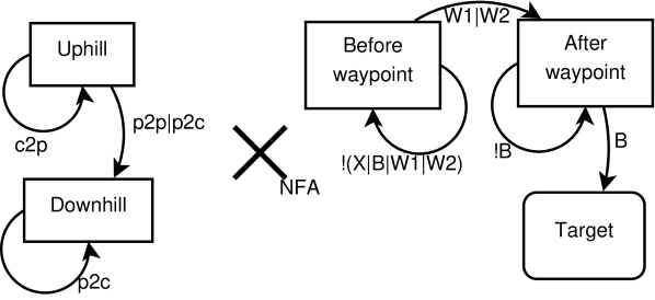
Figure 1: NFAs for the negative waypoint routing use case: valley-free (left side) and waypoint routing policies (right side).

Multipath TCP (MPTCP)

MPTCP [9] is a proposed extension to TCP from the IETF [10] allowing TCP connections to use multiple paths to increase resource utilization, redundancy and availability. This is especially useful when multiple wireless channels with different properties are available, or for better utilizing dense data center topologies, to exploit the large bisection bandwidth available. Consider the data center scenario, where the operator has full control over the endpoints and switches and can route subflows individually. Here, the number of disjoint available paths that MPTCP can send traffic over is useful information for the MPTCP implementation. Path diversity calculations in this case yield an approximation of the maximal number of distinct flows that MPTCP can push in the network without these flows contending with each other for bandwidth. The approach for calculating the effective path diversity can take into account domain-specific policies which have been, e.g., expressed via Merlin [7]. In addition, it enables data center operators to compute the policy-compliant available bandwidth between two areas of a network. This can help to estimate the time that a MPTCP bulk data transfer may require, or whether the network is utilized properly during the transfer.

DDoS Link-Flooding Attacks

Estimating the bisection bandwidth of a data center can lead to an approximation of the attack budget that a DDoS link-flooding attack against data center core links, such as Crossfire [11], may require. The recent attack against Spamhaus [12] indicates that such information is valuable both for the attacker and the defender: the attacker tries to find weak links which he can deplete at minimal cost, isolating entire domains from the Internet [11], while the defender tries to increase the cost for the attacker via suitable network and traffic engineering [13]. Knowing how much bandwidth needs to be depleted to cut off a network from the rest of the Internet can help an operator perform an informed risk assessment of a possible attack, while taking into account the routing policies imposed over the network.

III Idea: Custom Graph Transform

Our objective is to transform a directed labelled graph $G$ into another graph $G^{\prime}$, such that: (i) only policy-compliant paths exist in $G^{\prime}$, and (ii) the transformation does not distort the minimum cut. The minimum cut may represent either bisection bandwidth or, by choosing unitary edge capacities, path diversity (cf. Menger’s theorem [1]). We define a policy-compliant path as any path whose path string (the string resulting from concatenating the edge labels) belongs to some regular language $L$. How do we accomplish this? Every regular language $L$ is represented by a finite state automaton $M$, and vice versa. Therefore, upon traversing an edge in the graph, we need to accordingly change the state in the automaton, as if the edge label had been given to the automaton as an input.

The first idea is to use the tensor product of the graph $G$ and the policy-checking automaton $M$ (Fig. 2 gives an example). From $M$ we define the transition graph $T$, which has a node set consisting of the states of $M$ and an edge set representing the permitted state transitions of $M$. The edges in $G$ and $T$ are labelled with policy-related symbols that result in the state transitions represented in $T$. For each of these symbols $s\in\Sigma$, we form the subgraphs $G_{s}$ and $T_{s}$ consisting of all the edges labelled with $s$. We then form the tensor product of these subgraphs, which is defined as follows: if $v_{1}$ and $v_{2}$ are nodes in $G$ and $q_{1}$ and $q_{2}$ are nodes in $T$, then $G^{\prime}$ contains the nodes $(v_{1},q_{1})$, $(v_{1},q_{2})$, $(v_{2},q_{1})$ and $(v_{2},q_{2})$. Likewise, if there is an edge $(v_{1},v_{2})$ in the subgraph $G_{s}$ and an edge $(q_{1},q_{2})$ in the subgraph $T_{s}$, then the tensor product contains the edge $((v_{1},q_{1}),(v_{2},q_{2}))$. The union of all of these tensor products is the transformed graph $G^{\prime}$. This allows us to move both between the nodes $v_{1}$ and $v_{2}$ in $G$ and the nodes $q_{1}$ and $q_{2}$ in $T$ (and therefore the states $q_{1}$ and $q_{2}$ in $M$) at the “same time”. We define $M$ to be a Non-deterministic Finite state Automaton (NFA) because an NFA is typically smaller than a corresponding Deterministic Finite state Automaton (DFA).

This transform gives us part of the solution, but it does not guarantee that the minimum cut calculated over $G^{\prime}$ represents accurately the corresponding minimum cut of $G$. A single edge in the original graph $G$ may be mapped to a set of parallel edges in the transformed graph $G^{\prime}$. Consider the possibility of a transition from one state $\{q_{1}\}$ to two states $\{q_{2},q_{3}\}$ over an edge $(v_{1},v_{2})$. This will be mapped to two edges in $G^{\prime}$: $((v_{1},q_{1}),(v_{2},q_{2}))$ and $((v_{1},q_{1}),(v_{2},q_{3}))$, even though there is just one edge in $G$. Therefore, the second idea is to force the transform to maintain the minimum cut. This may not always be possible, as we will explain later. If it is not, the result still is an approximation of the minimum cut, for which we will give lower and upper bounds in section IV-D.

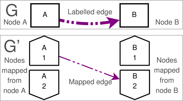
(a) Original$\rightarrow$Transformed Graph

(b) NFA

Figure 2: The tensor product. For each label $s\in\Sigma$, the tensor product of the edges in $G$ labelled with $s$ and the edges in $T$ labelled with $s$ (representing the state transitions in $M$ when $s$ is entered as an input) yields the set of mapped edges in $G^{\prime}$. We represent the edge label $s$ symbolically via the colour and style of the edge. Nodes in $G^{\prime}$ are derived from the triangles of the NFA and the squares of the original graph $G$.

The core idea is to add aggregator states to the NFA and consequently to $G^{\prime}$ so that the min-cut paths between two nodes must traverse at most the same number of parallel edges as in $G$, which limits the minimum cut in $G^{\prime}$ to the same value as in $G$. To preserve the structure of the NFA—and thus the policy it describes—we utilize $\varepsilon$-transitions. $\varepsilon$-transitions can be thought of as “free” transitions: they do not consume a symbol during traversal. In our case, this means that we do not need to traverse an edge between nodes in $G$ in order to traverse an $\varepsilon$-transition. Where there is a chance of the min-cut being inflated, we add an aggregator node (for each edge label) and use $\varepsilon$-transitions to “channel” all of the paths through this node. Each node in $G$ has corresponding aggregator nodes in $G^{\prime}$ as needed and where it is applicable.

There are several possible cases for the aggregated transitions: (i) from a single state to another single state (one-to-one), (ii) from a single state to multiple states (one-to-many), (iii) from multiple states to a single state (many-to-one), or (iv) from multiple states to multiple states (many-to-many). In the first case, the min-cut is always invariant; no inflation can occur. The latter cases are depicted in Fig. 3, Fig. 4, and Fig. 5, respectively. In the one-to-many and many-to-one cases the addition of aggregation nodes leads to the correct min-cut value, while the many-to-many case requires careful consideration. In this case, we can only maintain the accurate min-cut using aggregation states if the set of state transitions can be expressed as the Cartesian product of two subsets of the set of state nodes. This results in complete bipartite subgraphs on the transformed graph $G^{\prime}$ with aggregatable transitions, as shown in Fig. 5. Therefore, if this is not the case, we need to break the transition down to $n$ disjoint state transition sets of the cases (i) to (iv) and perform the transform for each of them; each set introduces an extra aggregator state. Regarding edge capacities we provide different values to yield upper and lower bounds on the min-cut, as we will show later.

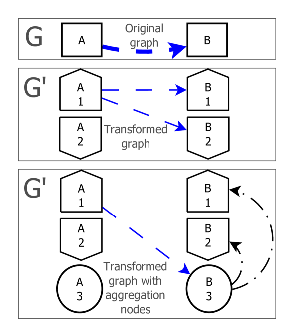
(a) Original$\rightarrow$Transformed Graph

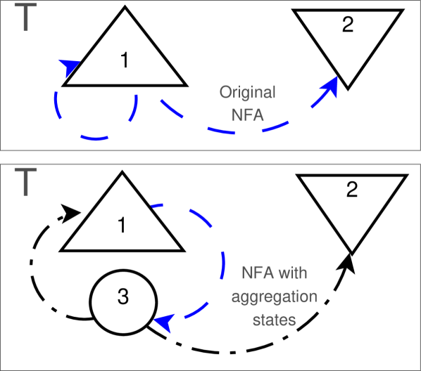
(b) NFA

Figure 3: The use of aggregation nodes (represented with circles) for a one-to-many state mapping. The two blue dashed transitions of the NFA are aggregated using one aggregation node. $\varepsilon$-transitions are represented by black dotted dashed lines.

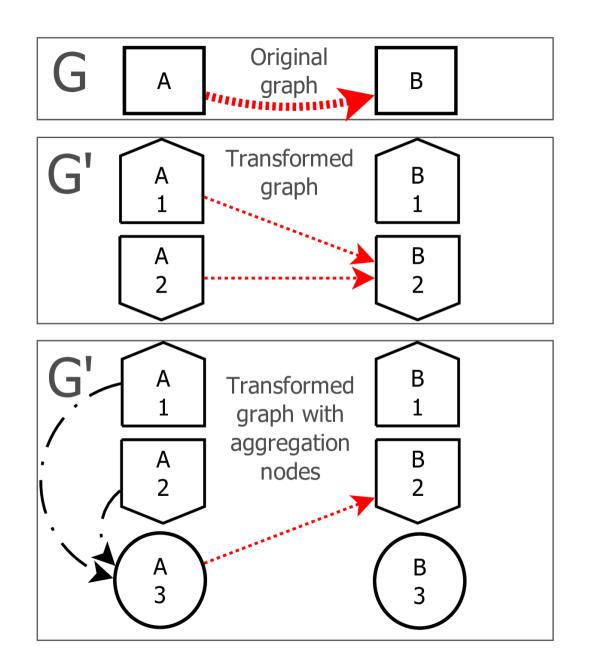
(a) Original$\rightarrow$Transformed Graph

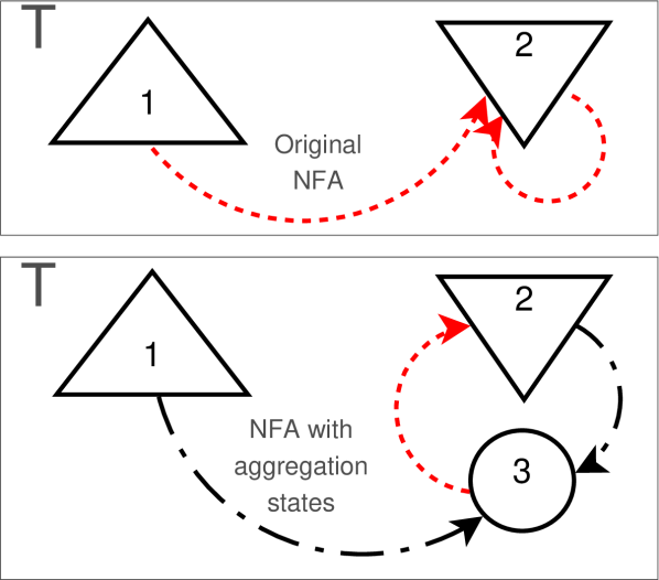
(b) NFA

Figure 4: The use of aggregation nodes (represented with circles) for a many-to-one state mapping. The two red dotted transitions of the NFA are aggregated using one aggregation node.

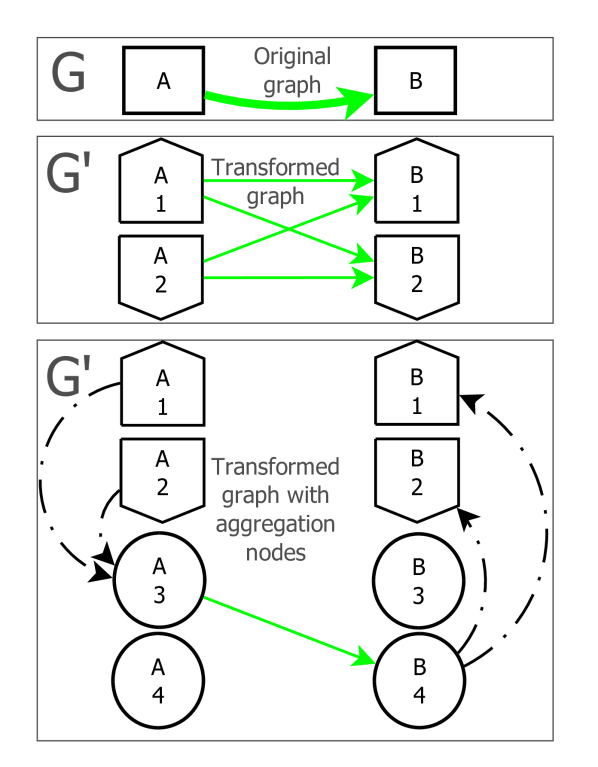
(a) Original$\rightarrow$Transformed Graph

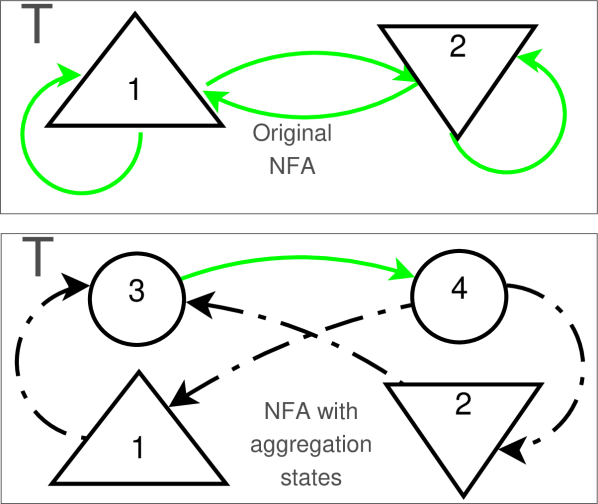
(b) NFA

Figure 5: The use of aggregation nodes for a many-to-many state mapping. The four green transitions of the NFA are aggregated using two aggregation nodes.

To calculate the min-cut with conventional algorithms, we need to have a single terminating node in $G^{\prime}$, which implies a single terminating state in $M$. If we have more than one terminating state, then prior to proceeding we need to create a virtual terminating state and copy all of the transitions to the previous terminating states to the new one. Finally, if we want to consider constraints on nodes as well as edges, we can split the nodes under consideration in two halves as follows: all of the incoming edges connect to one half and all of the outgoing edges connect to the other. We then add a labelled edge between those halves, allowing the edge to represent the node and effectively encompass its constraints.

IV The Math Behind the Transform

Here we present the required definitions, algorithmic steps, proofs of correctness, and complexity of the algorithm.

IV-A Notation and Definitions

• $G=(V,E)$ is a labelled directed graph with nodes $V$, edges $E$, a labelling function $l:E\rightarrow\Sigma$ that maps edges in $E$ to corresponding labels in $\Sigma$, and a capacity function $c:E\rightarrow\mathbb{R}^{+}$ that maps edges to edge capacities. For path diversity calculations, we choose $c(e)=1$ for all $e\in E$.

• $L\subseteq\Sigma^{*}$ is a regular language. We require that for any path $(e_{1},...,e_{n})$ in $G$, the string $l(e_{1})...l(e_{n})$ formed of the edge labels be in $L$.

• $M=(Q,\Sigma,\Delta,q_{0},F)$ is a NFA with states $Q$, input symbols $\Sigma$, state transitions $\Delta\subseteq Q\times\Sigma\times Q$, terminating states $F\subseteq Q$ and a starting state $q_{0}\in Q$. $M$ accepts $L$. $\varepsilon$-transitions are allowed with $\varepsilon\in\Sigma$.

• $T=(Q,\Delta)$ is the directed graph derived from $M$.

• $G^{\prime}=(V^{\prime},E^{\prime})$ is the final transformed graph: its formation is such that the policy constraints are met and the minimum cut is not inflated, if possible.

IV-B Single Virtual Termination States

In order to have a single terminating node in $G^{\prime}$ for use with Ford-Fulkerson (or another flow algorithm), the set of terminating states $F$ in $M$ must be no larger than one. If $|F|>1$, we add a new termination state $q^{*}$. A state transition to $q^{*}$ is added from every other state which previously had a transition to a terminating state, and $F$ is updated accordingly:

$$Q:=Q\cup\{q^{*}\}$$ (1)

$$\Delta:=\Delta\cup\{(q^{\prime},s,q^{*})\mid(q^{\prime},s,q)\in\Delta\wedge q\in F\}$$ (2)

$$F:=\{q^{*}\}$$ (3)

IV-C Tensor Product Transform: Steps

1. We form subgraphs $G_{s}\subseteq G$ consisting of all the edges labelled with $s\in\Sigma$:

   $$G_{s}:=(V,E_{s})$$ (4)

   $$E_{s}:=\{(v_{1},v_{2})\mid(v_{1},v_{2})\in E\wedge l((v_{1},v_{2}))=s\}$$ (5)

2. We form subgraphs $T_{s}\subseteq T$ of all the state transitions for an input symbol $s\in\Sigma$:

   $$T_{s}:=(Q,\Delta_{s})$$ (6)

   $$\Delta_{s}:=\{(q_{1},q_{2})\mid(q_{1},s^{\prime},q_{2})\in\Delta\wedge s^{\prime}=s\}$$ (7)

3. We augment $\Delta_{s}$ with aggregator states, if necessary. (i) We require that $\Delta_{s}$ has the form $Q^{\prime}_{s}\times Q^{\prime\prime}_{s}$ with $Q^{\prime}_{s}\subseteq Q$ and $Q^{\prime\prime}_{s}\subseteq Q$. (ii) If this is not the case, we decompose $\Delta_{s}$ into $n_{s}$ disjoint sets $\Delta_{s,k}$ such that each subset has the form $Q^{\prime}_{s,k}\times Q^{\prime\prime}_{s,k}$ and repeat the following for every $k$:

   1. We add a new aggregator state $q^{\prime}_{s}$ if $|Q^{\prime}_{s}|>1$ and $q^{\prime\prime}_{s}$ if $|Q^{\prime\prime}_{s}|>1$:

      $$Q:=\left\{\begin{array}[]{l l}Q&|Q^{\prime}_{s}|=1\\ Q\cup\{q^{\prime}_{s}\}&|Q^{\prime}_{s}|>1\end{array}\right.$$ (8)

      $$Q:=\left\{\begin{array}[]{l l}Q&|Q^{\prime\prime}_{s}|=1\\ Q\cup\{q^{\prime\prime}_{s}\}&|Q^{\prime\prime}_{s}|>1\end{array}\right.$$ (9)

   2. If we added a $q^{\prime}_{s}$ in the previous step, we connect the preceding states to it with an $\varepsilon$-edge. Likewise for $q^{\prime\prime}_{s}$ and succeeding states:

      $$\Delta_{\varepsilon}:=\left\{\begin{array}[]{l l}\Delta_{\varepsilon}&|Q^{\prime}_{s}|=1\\ \Delta_{\varepsilon}\cup(Q^{\prime}_{s}\times\{q^{\prime}_{s}\})&|Q^{\prime}_{s}|>1\end{array}\right.$$ (10)

      $$\Delta_{\varepsilon}:=\left\{\begin{array}[]{l l}\Delta_{\varepsilon}&|Q^{\prime\prime}_{s}|=1\\ \Delta_{\varepsilon}\cup(\{q^{\prime\prime}_{s}\}\times Q^{\prime\prime}_{s})&|Q^{\prime\prime}_{s}|>1\end{array}\right.$$ (11)

   3. Finally, we connect states $q^{\prime}_{s}$ and $q^{\prime\prime}_{s}$ with the aggregated state transition edge. If we did not use aggregating nodes on either side because there was only one state in $Q^{\prime}_{s}$ or $Q^{\prime\prime}_{s}$, we use that single state instead:

      $$Q^{\prime}_{s}:=\left\{\begin{array}[]{l l}Q^{\prime}_{s}&|Q^{\prime}_{s}|=1\\ \{q^{\prime}_{s}\}&|Q^{\prime}_{s}|>1\end{array}\right.$$ (12)

      $$Q^{\prime\prime}_{s}:=\left\{\begin{array}[]{l l}Q^{\prime\prime}_{s}&|Q^{\prime\prime}_{s}|=1\\ \{q^{\prime\prime}_{s}\}&|Q^{\prime\prime}_{s}|>1\end{array}\right.$$ (13)

      $$\Delta_{s}=Q^{\prime}_{s}\times Q^{\prime\prime}_{s}$$ (14)

4. For each pair of $G_{s}$ and $T_{s}$ that we derived in the previous steps, we calculate the tensor product $G^{\prime}_{s}=G_{s}\times T_{s}$. The nodes of $G_{s}^{\prime}$ are given by:

   $$V^{\prime}:=V\times Q$$ (15)

   The edges of $G_{s}^{\prime}$ are given by:

   $$E^{\prime}_{s}:=\{((v_{1},q_{1}),(v_{2},q_{2}))$$

   $$\mid(v_{1},v_{2})\in E_{s}\wedge(q_{1},q_{2})\in\Delta_{s}\}$$ (16)

   Furthermore, $\varepsilon$-transitions are mapped to edges in $G^{\prime}$ that are effectively located within a single node in $G$:

   $$E^{\prime}_{\varepsilon}:=\{((v,q_{1}),(v,q_{2}))\mid v\in V\wedge(q_{1},q_{2})\in\Delta_{\varepsilon}\}$$ (17)

5. $G^{\prime}$ is the union of $G^{\prime}_{s}$ for each $s\in\Sigma$ (including $\varepsilon$):

   $$G^{\prime}:=\bigcup_{s\in\Sigma}G^{\prime}_{s}=(V^{\prime},\bigcup_{s\in\Sigma}E^{\prime}_{s})$$ (18)

6. For the edge capacities $c^{\prime}:E^{\prime}\rightarrow\mathbb{R}^{+}$ in $G^{\prime}$, we have different values for the upper and lower bound minimum cut. (19) and (20) give the capacities $c^{\prime}_{upper}$ and $c^{\prime}_{lower}$ for the upper and lower bound minimum cuts, respectively.

   $$c^{\prime}_{upper}(((v_{1},q_{1}),(v_{2},q_{2})))=\left\{\begin{array}[]{l l}c(v_{1},v_{2})&v_{1}\neq v_{2}\\ \infty&v_{1}=v_{2}\\ \end{array}\right.$$ (19)

   $$c^{\prime}_{lower}(((v_{1},q_{1}),(v_{2},q_{2})))=\left\{\begin{array}[]{l l}\frac{c(v_{1},v_{2})}{n_{s}}&v_{1}\neq v_{2}\\ \infty&v_{1}=v_{2}\\ \end{array}\right.$$ (20)

   Where $s=l((v_{1},v_{2}))$ and $n_{s}$ is the number of disjoint sets $\Delta_{s,k}$ that $\Delta_{s}$ is decomposed into in step 3.

IV-D Correctness

We next prove that the transformed graph contains only valid policy-compliant paths (claims 1 and 2), that capacities $c^{\prime}_{lower}$ and $c^{\prime}_{upper}$ yield lower and upper bounds of the min-cut (claims 3 and 4), and that we obtain an exact value for the policy-compliant min-cut as long as certain conditions hold, pertaining to the form of the NFA (claim 5).

Claim 1.

Given a path $P$ in $G$, if the string formed by the concatenation of the edge labels of $P$ is not in $L$, then no corresponding path $P^{\prime}$ exists in $G^{\prime}$.

Proof.

The edge labels of $P$ form a string. This string contains at least one edge $e$ with a label $s\in\Sigma$ which results in the string no longer being in $L$. This implies that there is no outgoing state transition from the preceding state to any other state in the NFA. The tensor product of the NFA with the edge $e$ is thus empty. Therefore, there is no edge to the next node mapped from $P$ and no $P^{\prime}$ can be formed in $G^{\prime}$. ∎

Claim 2.

If a path $P$ exists in $G$ and the string formed by the concatenation of the edge labels of $P$ is in $L$, then there exists a corresponding path $P^{\prime}$ in $G^{\prime}$.

Proof.

If the edge labels traversed by $P$ form a string in $L$, then that string represents a sequence of valid state transitions in NFA $M$ (respectively the NFA graph $T$) from the starting to a terminating state. The tensor product for each $s\in\Sigma$ gives us a connection between two nodes if the edge corresponds to a valid state transition in $M$. As the string is in $L$, we know that all of the edge transitions are valid and therefore that all of the nodes mapped from $P$ to $P^{\prime}$ are connected. Thus a valid path $P^{\prime}$ can be formed in $G^{\prime}$. ∎

Claim 3.

Let $v_{1}$ and $v_{n}$ be nodes in $G$. Let $q_{0}$ and $q_{t}$ be the starting and terminating states in the NFA. Let the edge capacities of $G^{\prime}$ be $c^{\prime}_{lower}$ of (19). Then the minimum cut between $(v_{1},q_{0})$ and $(v_{n},q_{t})$ in $G^{\prime}$ is less than or equal to the minimum cut between $v_{1}$ and $v_{n}$ in $G$, taking into consideration only those paths whose edge labels form strings in $L$.

Proof.

From Claim 1 and Claim 2 we have that any path in $G^{\prime}$ corresponds to a valid path in $G$, and vice versa. For each pair of adjacent nodes $v_{k}$ and $v_{k+1}$ in the path in $G$ we have the capacity $c((v_{k},v_{k+1}))$ for the edge that connects them. The edge $(v_{k},v_{k+1})$ is mapped to $n_{s}$ edges in $G^{\prime}$, each having a capacity of $\frac{c((v_{k},v_{k+1}))}{n_{s}}$, where $n_{s}$ is the number of disjoint sets $\Delta_{s,k}$ that $\Delta_{s}$ is decomposed into in step 3. All of these $n_{s}$ mapped edges in $G^{\prime}$ therefore have a cumulative capacity of $c((v_{k},v_{k+1}))$, the same as between the pair of nodes in $G$ that they were mapped from. Hence the minimum cut between each pair of nodes in the path in $G^{\prime}$ is at most as large as that in $G$, while it may also be smaller due to the $\Delta_{s}$ decomposition. By induction, this applies to the path as a whole, and by generalization to all paths in $G^{\prime}$. Therefore, the minimum cut will not be overestimated and the calculated value in $G^{\prime}$ is a lower bound of the actual min-cut in $G$. ∎

Claim 4.

Let $v_{1}$ and $v_{n}$ be nodes in $G$. Let $q_{0}$ and $q_{t}$ be the starting and terminating states in the NFA. Let the edge capacities of $G^{\prime}$ be $c^{\prime}_{upper}$ of (20). Then the minimum cut between $(v_{1},q_{0})$ and $(v_{n},q_{t})$ in $G^{\prime}$ is greater than or equal to the minimum cut between $v_{1}$ and $v_{n}$ in $G$, taking into consideration only those paths whose edge labels form strings in $L$.

Proof.

From Claim 1 and Claim 2 we have that any path in $G^{\prime}$ corresponds to a valid path in $G$, and vice versa. For each pair of adjacent nodes $v_{k}$ and $v_{k+1}$ in the path in $G$ we have the capacity $c((v_{k},v_{k+1}))$ for the edge that connects them. The edge $(v_{k},v_{k+1})$ is mapped to $n_{s}$ edges in $G^{\prime}$ which all have the capacity $c((v_{k},v_{k+1}))$, where $n_{s}$ is the number of disjoint sets $\Delta_{s,k}$ that $\Delta_{s}$ is decomposed into in step 3. Hence the capacity of an edge $e$ in $G$ and of any edge $e^{\prime}$ in $G^{\prime}$ that $e$ is mapped to is the same. All valid paths in $G^{\prime}$ therefore have at least the same minimum cut as the ones in $G$ from which they are mapped, while there may be several corresponding parallel paths in $G^{\prime}$ due to the $\Delta_{s}$ decomposition. Therefore, the minimum cut will not be underestimated and the calculated value in $G^{\prime}$ is an upper bound of the actual min-cut in $G$. ∎

Claim 5.

The lower bound of claim 3 and the upper bound of claim 4 coincide and the min-cut calculation is exact if:

$$\forall s\in\Sigma:\exists Q^{\prime}_{s},Q^{\prime\prime}_{s}\subseteq Q:\Delta_{s}=Q^{\prime}_{s}\times Q^{\prime\prime}_{s}$$ (21)

Proof.

If (21) is true, then $n_{s}$ is equal to one for every $s\in\Sigma$. Accordingly, $c^{\prime}_{lower}(e)=c^{\prime}_{upper}(e)$ for every $e\in E^{\prime}$. This means that the lower and upper bounds of the minimum cut are equal. Since the actual min-cut lies between these values, it must therefore be equal to the lower and upper bounds. ∎

IV-E The Maximal Biclique Generation Problem

The number of disjoint sets $\Delta_{s,k}$ that $\Delta_{s}$ is decomposed into in step 3 of the graph transform determines how far off the lower and upper min-cut bounds are from the actual value in the worst case. Each $\Delta_{s,k}=Q^{\prime}_{s,k}\times Q^{\prime\prime}_{s,k}$ should be expressed as the Cartesian product of two state node subsets. The tensor product of each $\Delta_{s,k}$ with a link $(v_{i},v_{j})\in E_{s}$ is equivalent to a biclique in the transformed graph. This process can thus be reduced to finding the minimal number of complete bipartite graphs—or bicliques—that cover the transformed subgraph corresponding to the initial labelled link $(v_{i},v_{j})$. The found bicliques can then be used inversely to determine the $k$ $\Delta_{s,k}$ sets, i.e., to determine the Cartesian product decompositions of the NFA state transitions. This observation helps to estimate the complexity of the decomposition problem; though a formal analysis is outside the scope of this paper. The problem of finding maximal bicliques is generally $\mathsf{NP}$-Complete [14], and we refer the reader to existing literature for solutions [15, 16]. If looser bounds are acceptable, a heuristic solution could be used. We typically only need to decompose small subgraphs corresponding to simple NFAs and this only needs to be performed once per $\Delta_{s}$—i.e., per symbol— when transforming the graph. The time costs are significant only in cases where the NFA contains very large and complicated transitions. For many common scenarios, including 1-to-1, 1-to-N, N-to-1, and M-to-N, the decomposition is trivial (see Fig. 2 to 5).

IV-F Algorithmic Complexity

In Space

Here we consider the space complexity, which depends on the number of nodes and edges in graph $G$ and the number of states and transitions in NFA $M$. There are $|Q|$ states in the NFA. We may need to add $\mathcal{O}(|\Delta|)$ states for aggregation (at most one per transition). Therefore, applying the tensor product and taking into account the aggregation states gives us a total node complexity of:

$$|V^{\prime}|=\mathcal{O}(|V|(|Q|+|\Delta|))$$ (22)

Typically, one edge in $G$ will be mapped to one edge in $G^{\prime}$, plus some $\varepsilon$-edges. In the worst case, we may need $\mathcal{O}(|\Delta|)$ edges to map between two nodes (if many need to be decomposed into disjoint subsets in step 3). We may also need $\mathcal{O}(|\Delta|)$ $\varepsilon$-edges for each node, yielding a total edge complexity of:

$$|E^{\prime}|=\mathcal{O}(|\Delta|(|V|+|E|))$$ (23)

In Time

To obtain $G_{s}$, executing (5) requires $\Theta(|E|)$ steps (the nodes are maintained), while obtaining the $T_{s}$ requires executing (7), requiring $\Theta(|\Delta|)$ steps. Step 3 will be executed in the worst case $n$ times, where $n$ is the number of disjoint transition sets that $\Delta_{s}$ may be broken into, which cannot be larger than $|\Delta|$. Additionally, it demands $t_{dec}$ time, which is the amount of time required to actually decompose state transitions in $M$. The latter depends on $\Delta$, and may be of nondeterministic polynomial complexity. However, $t_{dec}$ is generally negligible in practice for many common scenarios (i.e., $|V|>>|Q|$ and $|E|>>|\Delta|$). 3a and 3c require only constant time, since they add a single object to a set. 3b requires $\mathcal{O}(|Q|)$ steps, giving us $\mathcal{O}(|Q||\Delta|)$ total time for step 3. For step 4, we have $\mathcal{O}(|V||Q|)$ for executing (15), $\mathcal{O}(|E||\Delta|)$ for executing (4) and $\mathcal{O}(|V||\Delta|)$ for executing (17). Finally, (18) requires $\mathcal{O}((|V|+|E|)|\Delta|)$ steps. Thus, the total time complexity is:

$$t=\mathcal{O}(|V||Q|+|\Delta|(|V|+|E|+|Q|))+t_{dec}$$ (24)

In practice, the total running time is dominated by the min-cut calculation on the transformed graph—e.g., via Ford-Fulkerson or Edmonds-Karp—rather than by the graph transformation process itself. The spatial complexity of the transformed graph in terms of the sizes $|V^{\prime}|$ and $|E^{\prime}|$ is the most important factor for the time that the min-cut calculation requires.

V Applications

In this section we showcase some of the applications of the graph transform algorithm. Note that our main contribution is the algorithm; here, we simply wish to demonstrate its applicability to a selection of real-world problems, rather than provide a full and rigorous analysis.

V-A Paths between tier one and tier two providers

Setup

We begin by calculating the number of edge-disjoint paths between some of the largest ISPs in the world, using the CAIDA AS relationships data [8]. We performed this calculation both for the total path diversity assuming no policies, i.e., arbitrary paths, and also for the diversity of valley-free paths using the regular expression described in Section II. We note that this regular expression can be mapped to an NFA that satisfies condition (21); therefore, the obtained values in this case are exact since the min-cut bounds coincide.

Results

The results are shown in Table I. The ISPs are: NTT (AS2914), Deutsche Telekom (AS3320), AT&T (AS7018), Embratel (AS4230), BT (AS5400) and Comcast (AS7922). First of all, we notice that unconstrained routing could offer around two orders of magnitude greater path diversity than the valley-free case. We observe substantial path diversity present between tier ones and tier twos, especially considering that these are AS-level paths, corresponding to multiple links at the router level. We note that the number of valley-free paths between pairs of tier one ISPs is always one due to the lack of an upstream ISP as well as the prohibition of traversing multiple peering links; thus we see only their direct p2p interconnections. The sizeable customer cone of the tier ones combined with this lack of diversity means that any depeering has the potential to cause major disruption for the direct tier one customers, which is known to have occurred already [17, 18]. For large tier twos, due to the rich peer-to-peer interconnectivity resulting in large path diversity, such depeerings seem not to be harmful. In this context we remark that even for very large ISPs, the limiting factor for path diversity is often the number of peering and provider connections that the ISP itself maintains, rather than the Internet topology at large; this points to a densely connected Internet. An ISP which wishes to improve its connectivity can therefore either establish a business relationship with another upper tier ISP, or expand its peering. Many evidently choose the latter [19], with the propagation of public open Internet Exchange Points (IXPs) [20] lowering the barriers to entry for establishing new peering relationships.

	Arbitrary paths						Valley-free paths
AS	2914	3320	7018	4230	5400	7922	2914	3320	7018	4230	5400	7922
2914	-	496	1012	190	145	145	-	1	1	9	5	2
3320	496	-	496	190	145	145	1	-	1	10	6	3
7018	1012	496	-	190	145	145	1	1	-	9	5	3
4230	190	190	190	-	145	145	9	10	9	-	10	8
5400	145	145	145	145	-	145	5	6	5	10	-	6
7922	145	145	145	145	145	-	2	3	3	8	6	-

TABLE I: Path diversity between large tier one and tier two ISPs. Tier one ISPs are marked in bold face for clarity.

V-B Global path diversity

Setup

To extend the previous use case, we look at the number of edge-disjoint paths between arbitrary pairs of ASes. We again use the CAIDA AS relationships data [8] and use the valley-free model. Due to the large number of ASes present, it is not feasible to calculate the pairwise path diversity for every pair of ASes. Instead we sample the ASes, selecting each AS with a probability proportional to the number of addresses it announces, using the CAIDA RouteViews AS-to-prefix data [21]. The AS relationships dataset is obtained from BGP routes announced at various vantage points within the Internet; the downside to this is that many peering links are not visible from these vantage points. In reality, the number of peering links in the Internet may be much larger than reported in this dataset [22]. To address this deficiency, we augment the AS relationships with data available from PeeringDB, which was evaluated and validated by Lodhi et al. [23]. We specifically add links between IXP members with an Open policy, indicating a general willingness to peer with other IXP members without any preconditions (such as balanced traffic). The majority of IXP members have an Open peering policy. In addition to the valley-free scenario, we also evaluate a more liberal policy, where a path may traverse more than one peering link between the uphill and downhill transitions. As we will see later, this can increase resiliency substantially. We note that the multiple peering link case corresponds also—like the classic valley-free case—to an NFA that satisfies condition (21), thus yielding exact values for the path diversity calculations.

Results

Fig. 6 shows the CCDF of path diversity. We evaluated the path diversity between 10,000 pairs of randomly selected ASes, with the selection weighted by the number of announced addresses as already described beforehand. We observe that (i) the added links make little difference to the valley-free scenario, (ii) the multiple peering links scenario has a considerably larger path diversity and profits a little more from extra peering links. Note that although the two valley-free scenarios appear to be identical, there are small differences between them hidden by the log scale, which we will see later.

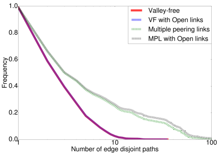
Figure 6: CCDF of path diversity, by constraint type and added link policy. VF: Valley-Free, MPL: Multiple Peering Links.

V-C Effects of peering policy openness on path diversity

Setup

Typically, IXP members have Open, Selective and Restrictive peering policies. The majority of IXP members have an Open policy, which, as stated above, implies the willingness to peer with other IXP members without any preconditions. A Selective policy generally implies certain preconditions, such as balanced traffic (e.g., a maximal 1:2 ratio) or geographically diverse peering points (e.g., one on every continent), and is typical for major ISPs. A Restrictive peering policy generally indicates the intent to peer only on a case-by-case basis, which is typical for the largest ISPs, especially tier ones. We would like to examine the effect of adding peering links from a given policy class in terms of the AS-level path diversity. While introducing peering links between all pairs of IXP members with an Open policy is a reasonable approach to augment the graph, the other cases may be less realistic. One approach is to add links between all pairs of IXP members sharing the same peering policy. ISPs typically peer with similarly sized ISPs, and peering policy may be seen as a crude indicator of ISP size (with larger ISPs being more restrictive).

Results

Table II shows the results of the path diversity calculation between 10,000 randomly selected pairs of ASes, with the selection weighted by the number of announced addresses. We observe that especially Open links increase the mean path diversity by 10.9%. This is not surprising given that: (i) these are the most numerous, and (ii) the most likely to be missed by BGP route collectors—relationships between the largest ISPs are most likely to be faithfully represented in the AS relationship dataset. Restrictive and Selective links—between IXP members with the same respective policy—have smaller impact on path diversity.

	Path diversity
Links added	$\mu$	$\sigma$
None	2.836	2.620
Restrictive	2.851	2.633
Selective	3.037	2.953
Open	3.146	3.136

(a) Policy

	Mean path diversity
Scenario	Before	After	Difference
Valley-free	1.100	1.023	7.03 %
+ Open links	1.101	1.023	7.02 %
Multiple peering links	1.267	1.267	0.02 %
+ Open links	1.499	1.499	0.04 %

(b) Depeering

TABLE II: The effect on path diversity of (i) augmenting the relationship graph with IXP membership data (values are not cumulative), by policy and (ii) depeering two tier one ISPs, by constraint type and whether or not the graph is augmented with IXP membership data. The values are rounded off.

V-D Effects of depeering on path diversity

Setup

We have already noted the effect of a depeering event, where one ISP chooses to cease sharing its routes with one of its peers. We would like to investigate the effect of such an event on path diversity. We synthetically create a depeering event by removing the peering between two tier ones, in this case Deutsche Telekom (AS3320) and Level3 (AS1, AS3356 and AS3549). We then evaluate the path diversity between the exclusive customer cones of the ISPs, i.e., the sets of customers which have only the one but not the other as (transit) upstream providers, and vice versa. We examine these customer cones down to a depth of three. As before, we also examine the effect of adding peering links. Now we also consider the possibility of a model more liberal than valley-free, allowing to traverse multiple peering links, as examined also by Hu et al. [24] and Kotronis et al. [25]. We evaluate the effect of allowing this while still maintaining the overall valley-free model (i.e., not permitting a provider to transit via its customers).

Results

Table II shows the results of the depeering for the different scenarios involving 10,000 pairs of ASes, selected pairwise from each of the tier one AS’s exclusive customer cones. For the valley-free model, we observe a negligible increase in path diversity by adding the extra links from PeeringDB, both before and after the depeering. The depeering event causes an approximately $7\,\%$ decrease in path diversity. Conversely, if we allow multiple peering links, the addition of the extra peering links boosts path diversity by over $18\,\%$. Here we do not observe a significant drop in path diversity due to the depeering. Allowing multiple peering links can therefore potentially increase resilience in the face of a depeering.

VI Related Work

Tensor Products

Soulé et al. [7] use a similar process to the one presented in this paper in the context of network management. Their goal is to enforce bandwidth allocation subject to path constraints represented by regular expressions and consequently by NFAs. They use tensor products in a different context than our approach, since we focus on path diversity and the implications arising in its preservation across transformations. In particular, we further propose the addition of aggregator nodes, acting as inhibitors to min-cut inflation.

Network Resilience

Previous research on resilient networks [26, 27] considers the network as a set of nodes and links, annotated with geographical properties. Consequently, researchers can calculate min-cuts, path distances or shared fate link groups that are affected in a correlated fashion during a disaster. On the other hand, networks are run as policy-compliant administrative domains [3]; the choice of paths that traffic can traverse is constrained. The view of the network as a geographical map cannot capture this behavior. Thus, we argue that network resilience should be also estimated under a policy-compliance framework. Our approach enables exactly that, allowing to run vanilla min-cut calculation algorithms like Ford-Fulkerson on the transformed graph, with tight min-cut approximations under certain conditions.

Min-cuts with Policies

Sobrinho et al. [28] describe a model for understanding the connectivity provided by route-vector protocols in the face of routing policies. Erlebach et al. [29, 30] study valid s-t-paths and s-t-cuts in the valley-free model and prove the NP-hardness of the vertex-disjoint min-cut problem. On the other hand, they prove that the edge-disjoint version can be solved in polynomial time for valley-free policies; we have verified this statement in our framework. Both works focus on specific aspects of the general problem (route-vector protocols and valley-free policies respectively), while we are delving into a more general methodology for min-cut estimations. Sobrinho et al. [28] examine the dynamics of a routing protocol with their work, while we concentrate on a general method to understand the effect of stable network policies on path diversity, ignoring for example the dynamics of routing convergence. Teixeira et al. [31] study vertex- and edge-disjoint paths in undirected Internet topology models, but without taking routing policies into account.

VII Conclusion

Path diversity and bisection bandwidth are useful metrics to describe how resilient or rich a network is. Network policies, imposed by network administrators and applied via routing protocols or network configuration, can constrain the natural path diversity of a network graph. With this work, we described and proved the correctness of a generic methodology for min-cut computations in arbitrary graphs, assuming policies that can be formulated using regular expressions. Our approach can be applied in a variety of scenarios, some of which are briefly showcased in this paper. These include the investigation of Internet topology and alternative policy models in the Internet, effectively studying Internet-wide resilience and the effects of inter-AS connectivity on path diversity. We see further potential for our approach in the analysis of MPTCP flow path availability in data center networks, and path selection optimization in multipath flow routing applications. Achieving tighter bounds for the min-cut is another topic of interest.

VIII Acknowledgements

We would like to thank Dr. Stefan Schmid (TU Berlin) for his valuable advice, as well as the anonymous reviewers for their feedback. This work has received funding from the European Research Council Grant Agreement n. 338402.

References

- [1] S. L. Arlinghaus, W. C. Arlinghaus, and F. Harary, Graph Theory and Geography: an Interactive View. Wiley New York, 2001.
- [2] W. Xu and J. Rexford, “MIRO: Multi-path Interdomain Routing,” in Proceedings of ACM SIGCOMM, 2006.
- [3] M. Caesar and J. Rexford, “BGP Routing Policies in ISP Networks,” Network, IEEE, vol. 19, no. 6, pp. 5–11, 2005.
- [4] L. Gao and J. Rexford, “Stable Internet Routing Without Global Coordination,” IEEE/ACM TON, vol. 9, no. 6, pp. 681–692, 2001.
- [5] A. Brüggemann-Klein, “Regular Expressions into Finite Automata,” Theoretical Computer Science, vol. 120, no. 2, pp. 197–213, 1993.
- [6] L. Ford and D. R. Fulkerson, Flows in Networks, vol. 1962. Princeton University Press, 1962.
- [7] R. Soulé, S. Basu, R. Kleinberg, E. G. Sirer, and N. Foster, “Managing the Network with Merlin,” in Proceedings of ACM HotNets, 2013.
- [8] “The CAIDA AS Relationships Dataset.” http://www.caida.org/data/as-relationships/. Dataset used: 2013-11-01.
- [9] H. Han, S. Shakkottai, C. Hollot, R. Srikant, and D. Towsley, “Multi-Path TCP: A Joint Congestion Control and Routing Scheme to Exploit Path Diversity in the Internet,” IEEE/ACM TON, vol. 14, no. 6, pp. 1260–1271, 2006.
- [10] A. Ford, C. Raiciu, M. Handley, and O. Bonaventure, “TCP Extensions for Multipath Operation with Multiple Addresses.” RFC 6824 (Experimental), Jan. 2013.
- [11] M. S. Kang, S. B. Lee, and V. D. Gligor, “The Crossfire Attack,” in Proceedings of the 2013 IEEE Symposium on Security and Privacy, 2013.
- [12] M. Prince, “The DDoS That Knocked Spamhaus Offline (And How We Mitigated It).” (Mar. 20, 2013, 06:26 PM), CloudFlare Blog, 2013.
- [13] S. T. Chow, D. Wiemer, and J.-M. Robert, “Distributed Defence Against DDoS Attacks,” July 5 2007. US Patent App. 11/822,341.
- [14] R. Peeters, “The Maximum Edge Biclique Problem is NP-complete,” Discrete Appl. Math., vol. 131, no. 3, pp. 651–654, 2003.
- [15] E. Kayaaslan, “On Enumerating All Maximal Bicliques of Bipartite Graphs,” in Proceedings of CTW, 2010.
- [16] D. Binkele-Raible, H. Fernau, S. Gaspers, and M. Liedloff, “Exact Exponential-time Algorithms for Finding Bicliques,” Information Processing Letters, vol. 111, no. 2, pp. 64 – 67, 2010.
- [17] T. Underwood, “Wrestling With the Zombie: Sprint Depeers Cogent, Internet Partitioned.” (Oct. 31, 2008, 10:07 AM), Renesys Blog, 2008.
- [18] M. A. Brown, A. Popescu, and E. Zmijewski, “Peering Wars: Lessons Learned From the Cogent-Telia De-peering.” Presentation, Renesys Corp, New York, 2008.
- [19] N. Chatzis, G. Smaragdakis, A. Feldmann, and W. Willinger, “There is More to IXPs Than Meets the Eye,” SIGCOMM CCR, vol. 43, no. 5, pp. 19–28, 2013.
- [20] EuroIX: European Internet Exchange Association, “List of Known IXPS Around the Globe.” https://www.euro-ix.net/resources-list-of-ixps, 2014.
- [21] “Routeviews Prefix to AS mappings Dataset for IPv4 and IPv6.” http://www.caida.org/data/routing/routeviews-prefix2as.xml. Dataset used: 2014-01-11, 12:00 UTC.
- [22] B. Ager, N. Chatzis, A. Feldmann, N. Sarrar, S. Uhlig, and W. Willinger, “Anatomy of a Large European IXP,” SIGCOMM CCR, vol. 42, no. 4, pp. 163–174, 2012.
- [23] A. Lodhi, N. Larson, A. Dhamdhere, C. Dovrolis, et al., “Using peeringDB to Understand the Peering Ecosystem,” ACM SIGCOMM CCR, vol. 44, no. 2, pp. 20–27, 2014.
- [24] C. Hu, K. Chen, Y. Chen, and B. Liu, “Evaluating Potential Routing Diversity for Internet Failure Recovery,” in Proceedings of IEEE INFOCOM, 2010.
- [25] V. Kotronis, X. Dimitropoulos, R. Klöti, B. Ager, P. Georgopoulos, and S. Schmid, “Control Exchange Points: Providing QoS-enabled End-to-End Services via SDN-based Inter-domain Routing Orchestration,” in Proceedings of the Research Track of ONS 2014, 2014.
- [26] E. K. Çetinkaya, M. J. Alenazi, A. M. Peck, J. P. Rohrer, and J. P. G. Sterbenz, “Multilevel Resilience Analysis of Transportation and Communication Networks,” Springer Telecommunication Systems Journal, 2013.
- [27] Y. Cheng, J. Li, and J. P. G. Sterbenz, “Path Geo-diversification: Design and Analysis,” in Proceedings of IEEE/IFIP RNDM Workshop, 2013.
- [28] J. a. L. Sobrinho and T. Quelhas, “A Theory for the Connectivity Discovered by Routing Protocols,” IEEE/ACM Trans. Netw., vol. 20, no. 3, pp. 677–689, 2012.
- [29] T. Erlebach, A. Hall, A. Panconesi, and D. Vukadinović, “Cuts and Disjoint Paths in the Valley-free Path Model of Internet BGP Routing,” in Proceedings of CAAN, 2005.
- [30] T. Erlebach, L. S. Moonen, F. C. Spieksma, and D. Vukadinovic, “Connectivity Measures for Internet Topologies on the Level of Autonomous Systems,” Operations research, vol. 57, no. 4, pp. 1006–1025, 2009.
- [31] R. Teixeira, K. Marzullo, S. Savage, and G. M. Voelker, “Characterizing and Measuring Path Diversity of Internet Topologies,” in Proceedings of ACM SIGMETRICS, 2003.