Adjacency Graphs and Long-Range Interactions of Atoms in Quasi-Degenerate States: Applied Graph Theory

Abstract

We analyze, in general terms, the evolution of energy levels in quantum mechanics, as a function of a coupling parameter, and demonstrate the possibility of level crossings in systems described by irreducible matrices. In long-range interactions, the coupling parameter is the interatomic distance. We demonstrate the utility of adjacency matrices and adjacency graphs in the analysis of “hidden” symmetries of a problem; these allow us to break reducible matrices into irreducible subcomponents. A possible breakdown of the no-crossing theorem for higher-dimensional irreducible matrices is indicated, and an application to the $2S$–$2S$ interaction in hydrogen is briefly described. The analysis of interatomic interactions in this system is important for further progress on optical measurements of the $2S$ hyperfine splitting.

I Introduction

In quantum mechanical systems described by a ($2\times 2$)-matrix, no level crossings can typically occur Cohen-Tannoudji et al. (1978a, b). This is known as the “no level crossing theorem” and often illustrated on the basis of the simple $(2\times 2)$-model Hamiltonian matrix

$$H^{\prime}=H+P=\left(\begin{array}[]{cc}E_{1}&0\\ 0&E_{2}\end{array}\right)+\left(\begin{array}[]{cc}0&C\,g\\ C\,g&0\end{array}\right)\,,$$ (1)

where $E_{1}$ and $E_{2}$ are the unperturbed energy levels, $C$ is a parameter, and $g$ is the coupling constant. The energy levels are

$$E_{\pm}=\frac{1}{2}\,(E_{1}+E_{2})+\frac{1}{2}\,\sqrt{(E_{1}-E_{2})^{2}+4(C\,g)^{2}}\,.$$ (2)

As a function of $g$, one obtains two hyperbolas, with the distance of “closest approach” between the energy levels occurring for $g=0$, with a separation $|E_{+}-E_{-}|=|E_{1}-E_{2}|$. For a level crossing to occur at $g=0$, one has to have $E_{1}=E_{2}$. The larger the perturbation, the more the energy levels “repel” each other.

However, the situation is less clear for more complex systems involving more than two energy levels. To this end, we shall analyze a higher-rank matrix which describes energy levels some of which repel each other on the basis of inter-level couplings, in a system which obviously can be broken into smaller subcomponents (i.e., the Hamiltonian is a reducible matrix having irreducible submatrices). As the levels in the irreducible subsystems evolve from the weak-coupling to the strong-coupling regime, those coming from different irreducible submatrices cross. When additional couplings are introduced between the subsystems, the matrix becomes irreducible. In this case, we shall demonstrate that some of the level crossings are avoided, but not all. Our example will be based on a $(6\times 6)$-matrix.

Another question which sometimes occurs in the analysis of interatomic interactions, and other contexts in quantum mechanics, concerns the reducibility of a matrix. Reducible tensors are usually introduced in the context of the rotation group. Under a rotation, scalars transform into scalars, vectors transform into vectors, quadrupole tensors transform into quadrupole tensors, and so on. It means that a matrix representation of the rotation would have an obvious block structure when formulated in terms of the irreducible tensor components. For example, a trivially reducible matrix is

$$H^{\prime\prime}=\left(\begin{array}[]{ccc}E_{1}&C\,g&0\\[0.4878pt] C\,g&E_{2}&0\\[0.4878pt] 0&0&E_{3}\end{array}\right)\,,$$ (3)

as it can obviously be broken into an upper $(2\times 2)$ submatrix equal to $H^{\prime}$, and a lower $(1\times 1)$ submatrix just consisting of the uncoupled energy level $E_{3}$.

The question of whether a higher-dimensional matrix is reducible, can be far less trivial to analyze. For example, in a $(24\times 24)$ matrix, as has been recently encountered in our analysis of the $2S$–$2S$ hyperfine-resolved interactions in hydrogen Jentschura et al. (2016), entries can follow a rather irregular pattern, and the analysis then becomes far less trivial. The possibility to break up a matrix into irreducible subcomponents is equivalent to a search for “hidden” symmetries of the interaction which imply that only sublevels of specific symmetry are coupled.

After a brief look at level crossings in Sec. II, we continue with an analysis of irreducible (sub-)matrices in Sec. III. An application of the concepts developed to the $2S$–$2S$ hyperfine interaction in hydrogen is briefly described in Sec. IV.

II Couplings and Level Crossings

Let us consider the 6 x 6 matrix

$$H_{0}=\left(\begin{array}[]{cccccc}E_{1}&C_{1}\,g&C_{1}\,g&0&0&0\\ C_{1}\,g&E_{2}&C_{1}\,g&0&0&0\\ C_{1}\,g&C_{1}\,g&E_{3}&0&0&0\\ 0&0&0&E_{4}&0&0\\ 0&0&0&0&E_{5}&C_{1}\,g\\ 0&0&0&0&C_{1}\,g&E_{6}\end{array}\right)$$ (4)

This matrix consists of a mutually coupled (irreducible) upper $(3\times 3)$-block, an irreducible lower $(2\times 2)$-block, and one uncoupled state in the middle, with energy $E_{3}$. For the choice

$$E_{j}=j\,,\qquad C_{1}=1\,,$$ (5)

the evolution of the eigenenergies $E_{j}\to E_{j}(g)$ is analyzed in Fig. 1. Specifically, the level crossings occur at

$$E_{3}(g^{\prime})= \;E_{4}(g^{\prime})=4\,,\qquad g^{\prime}=0.879\,385\,,$$ (6a)

$$E_{3}(g^{\prime\prime})= \;E_{5}(g^{\prime\prime})=4.326\,328\,,$$

$$g^{\prime\prime}= \;1.061\,840\,,$$ (6b)

$$E_{4}(g^{\prime\prime\prime})= \;E_{5}(g^{\prime\prime\prime})=4,\qquad g^{\prime\prime\prime}=\sqrt{2}\,.$$ (6c)

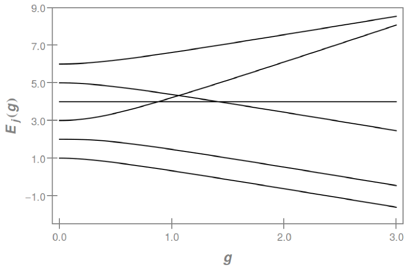
Figure 1: Evolution of the energy levels $E_{j}(g)$ of the matrix $H_{0}$ given in Eq. (4), for the parameter choice given in Eq. (5). One can clearly discern the mutual “repulsion” between the lowest three energy levels $E_{1,2,3}$, stemming from the upper $(3\times 3)$-block of the matrix (4), and the same repulsion among the highest energies $E_{4,5}$, stemming from the upper $(2\times 2)$-block of the matrix (4). The level crossings occur with respect to the uncoupled level $E_{3}$, which is independent of $g$.

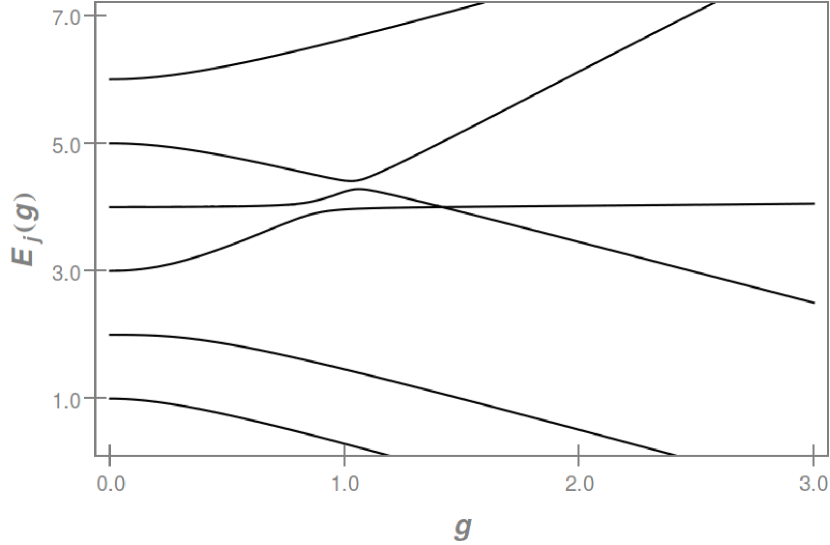
Figure 2: Evolution of the energy levels $E_{j}(g)$ of the matrix $H$ given in Eq. (8), for the parameter choices given in Eqs. (5) and (9). In comparison to Fig. 1, the ordinate axis is compressed in order to focus on the level crossings. The crossings (6a) and (6) have turned into anticrossings, in view of the mutual level repulsion as the inter-level couplings are introduced, in accordance with the no-crossing theorem. However, the crossing (6c) is retained (with a slightly different values of $g^{\prime\prime\prime}$), with the twist that it takes place between $E_{3}$ and $E_{4}$ this time (instead of $E_{4}$ and $E_{5}$ as in the previous case). This change is due to the fact that the crossing (6a) between $E_{3}$ and $E_{4}$ and the crossing (6) between $E_{3}$ and $E_{5}$ are now avoided.

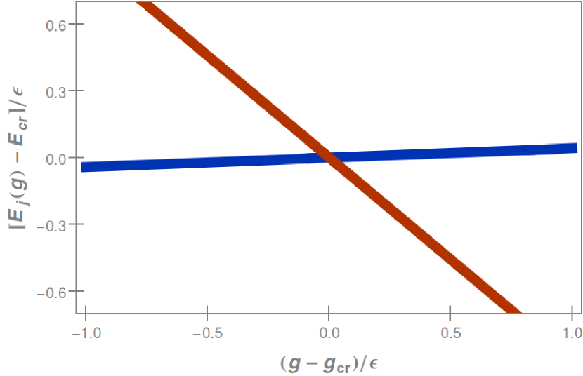
Figure 3: Close-up of Fig. 2 in the region $E_{3}(g)\approx E_{4}(g)\approx 4$, and $g\approx g_{\rm cr}=\sqrt{2}$, with $\epsilon=10^{-128}$. This plot was obtained using extended-precision arithmetic, using a computer algebra system Wolfram (1999). The observed numerical behavior is consistent with the persistence of the level crossing for the irreducible matrix.

Let us now add a further perturbation $H_{1}$,

$$H_{1}=\left(\begin{array}[]{cccccc}0&0&0&C_{2}\,g&0&C_{2}\,g\\ 0&0&0&0&0&0\\ 0&0&0&0&0&0\\ C_{2}\,g&0&0&0&0&0\\ 0&0&0&0&0&0\\ C_{2}\,g&0&0&0&0&0\end{array}\right)\,,$$ (7)

where $C_{2}$ is another parameter, to obtain the total Hamiltonian

$$H=H_{0}+H_{1}=\left(\begin{array}[]{cccccc}E_{1}&C_{1}\,g&C_{1}\,g&C_{2}\,g&0&C_{2}\,g\\ C_{1}\,g&E_{2}&C_{1}\,g&0&0&0\\ C_{1}\,g&C_{1}\,g&E_{3}&0&0&0\\ C_{2}\,g&0&0&E_{4}&0&0\\ 0&0&0&0&E_{5}&C_{1}\,g\\ C_{2}\,g&0&0&0&C_{1}\,g&E_{6}\end{array}\right)\,.$$ (8)

In the total Hamiltonian $H$, the previously uncoupled level $E_{4}$ is now coupled to the upper $(3\times 3)$ block by the term $C_{2}$, and an additional coupling between the lower $(2\times 2)$ block and the upper $(3\times 3)$ block is introduced in the extreme upper right and lower left corners of the matrices $H_{1}$ and $H$. In Fig. 2, we study the evolution of the energy levels of $H$ for the parameter choice

$$C_{2}=\frac{3}{10}\,.$$ (9)

It is clearly seen that the level crossings (6a) and (6) now turn into avoided crossings, while the crossing (6c) is retained, but now occurs between $E_{3}$ and $E_{4}$ and not between $E_{3}$ and $E_{4}$. This difference is due to the avoided crossings.

The value of the energy at the crossing occurs at the coupling $g=g_{\rm cr}$,

$$E_{\rm cr}=E_{3}(g_{\rm cr})=E_{4}(g_{\rm cr})=4\,,\qquad g_{\rm cr}=\sqrt{2}\,.$$ (10)

We have verified (see Fig. 3) that the crossing persists under the use of extended-precision arithmetic, where the parameter $\epsilon=10^{-128}$ (on the level of Fortran “hexadecuple precision”) is employed in a numerical calculation of the eigenvalue near the crossing point, in order to ensure that the persistence of the crossing is not an artefact due to an insufficient numerical accuracy in the calculation. One might otherwise conjecture that the “crossing” would turn into an “avoided crossing” when looking at the crossing point with finer numerical resolution.

For $C_{1}=1$, as a function of $C_{2}$, the eigenvectors at the degenerate eigenvalue $E_{\rm cr}=4$ (where the crossing occurs) can be determined analytically; they read as

$$v_{3}= \;\left(0,-\frac{C_{2}}{1+\sqrt{2}},-\frac{\sqrt{2}\,C_{2}}{1+\sqrt{2}},0,-\sqrt{2},1\right)\,,$$ (11a)

$$v_{4}= \;\left(0,-\frac{C_{2}}{1+\sqrt{2}},-\frac{\sqrt{2}\,C_{2}}{1+\sqrt{2}},1,0,0\right)\,.$$ (11b)

A comparison of Fig. 1 to Fig. 2 reveals that the crossing “actually” occurs between the levels $4$ and $5$. According to the adjacency graph in Fig. 5, the levels $4$ and $5$ are the most distant ones in comparison to the levels $2$ and $3$ which constitute the $C_{2}$-dependent “admixtures” at the crossing. According to Eq. (11), Furthermore, in the limit $C_{2}\to 0$, the eigenvectors $v_{3}$ and $v_{4}$ given in Eq. (11) have contributions only from the unperturbed levels $4$, $5$, and $6$; the latter are not directly coupled to the levels $2$ and $3$ in the adjacency graph in Fig. 5. Apparently, the no-crossing theorem discussed in Ref. wik does not hold for higher-dimensional matrices, while crossings in $2\times 2$ matrices are strictly avoided in view of this theorem (see Chap. 79 of Ref. Landau and Lifshitz (1958)).

A comparison of Figs. 1 and 2 reveals that the number of crossings is seen to be reduced for the case of the irreducible Hamiltonian matrix, but it is not zero.

III Finding Irreducible Submatrices

We shall briefly discuss how to establish, by a formal, generalizable, method, that the matrix given in Eq. (4) is reducible, while the matrix (8) is irreducible.

Let us look at a general $(n\times n)$ matrix and associate it with the flight plan of a specific airline, with a nonvanishing entry, equal to unity, at position $(i,j)$, denoting the existence of a direct flight between the cities $i$ and $j$. If the matrix element $(i,j)$ is zero, then no such direct connection exists. This matrix is known as the “adjacency matrix” $U$ of the airline connection. A nonvanishing entry at position $(i,i)$ could be interpreted as a “sightseeing flight” starting and ending at city $i$. There could be an indirect coupling between cities $i$ and $j$, if not by a direct flight, then via a connection through some city $k$. If there is a connection with one intermediate stop, then it is obvious that the square of the adjacency matrix will have a unit entry at position $(i,j)$. Nonzero entries in $U^{2}$ represent the cities that connect with connecting flights (one intermediate stop only). More specifically, the entries in the square of the adjacency matrix count the number of possibilities that one can fly from city $i$ to city $j$ with exactly one intermediate stop. If the airline serves $n$ airports and one cannot go from city $i$ to city $j$ with $n-1$ intermediate stops, then one cannot go city $i$ to city $j$ at all. One has exhausted the possibilities. Let $U$ denote the adjacency matrix. It means that if the matrix

$$A=\sum_{i=1}^{n}U^{i}=U+U^{2}+\ldots+U^{n}$$ (12)

still has a zero entry at position $(i,j)$, then the airline must be serving at least two disconnected sets of destinations; this in turn is equivalent to showing that the adjacency matrix is reducible. The algorithm for testing the reducibility of an input matrix $M$ is now clear. One replaces all nonzero entries in the input matrix $M$ by unity, obtaining the adjacency matrix $U$. One then calculates the accumulated adjacency matrix $A$ according to Eq. (12). If there are zero entries in $A$, then $M$ must be reducible.

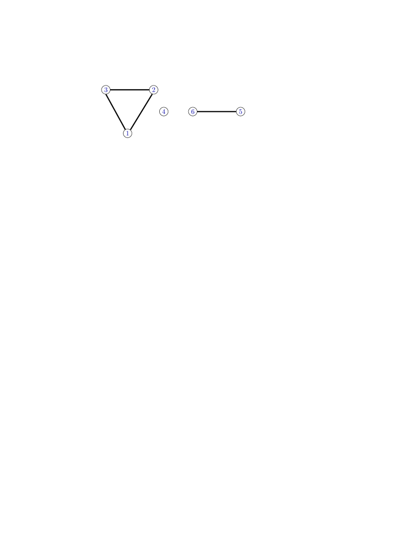
Figure 4: Adjacency graph for the matrix $U_{0}$ given in Eq. (13).

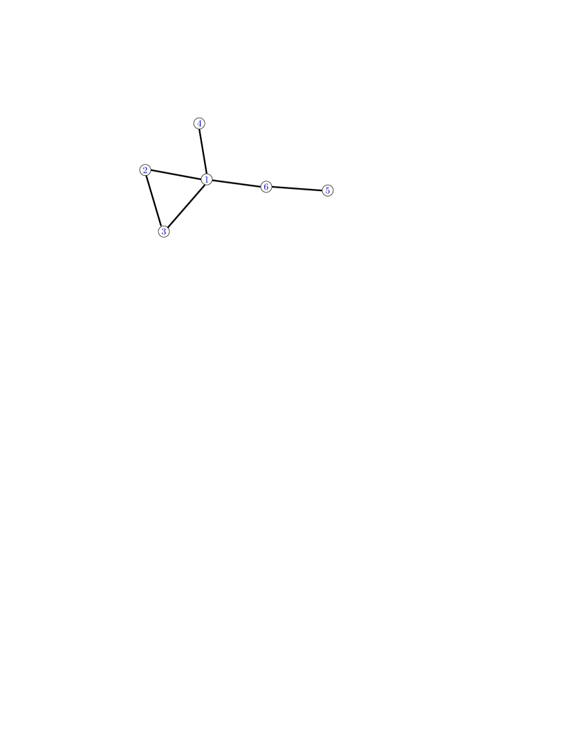
Figure 5: Adjacency graph for the matrix $U$ given in (15).

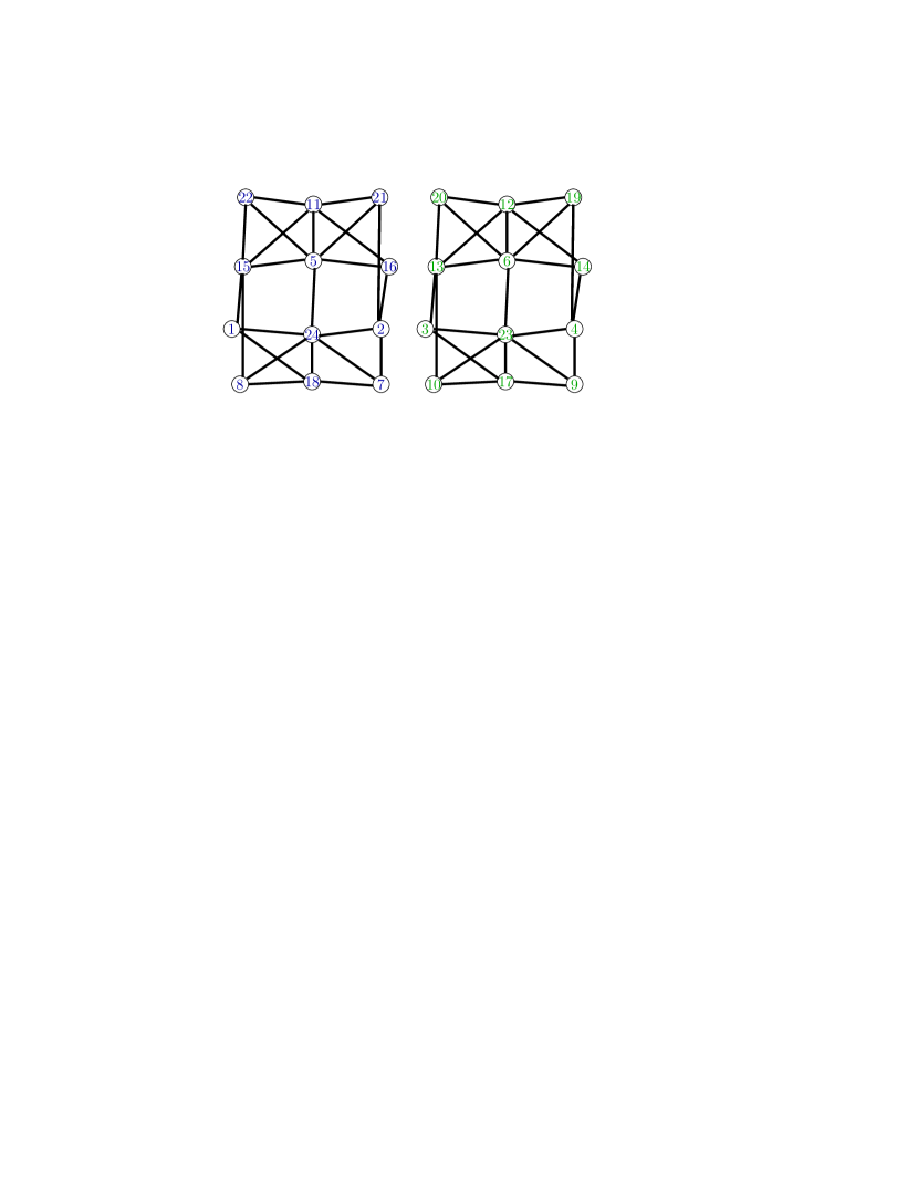
Figure 6: Adjacency graph for the matrix $U_{F_{z}=0}$ given in Eq. (24).

The adjacency matrix $U_{0}$ for $H_{0}$ given in Eq. (4) is

$$U_{0}=\left(\begin{array}[]{cccccc}1&1&1&0&0&0\\ 1&1&1&0&0&0\\ 1&1&1&0&0&0\\ 0&0&0&1&0&0\\ 0&0&0&0&1&1\\ 0&0&0&0&1&1\end{array}\right)\,,$$ (13)

resulting in

$$A_{0}=\sum_{i=1}^{6}U_{0}^{i}=\left(\begin{array}[]{cccccc}364&364&364&0&0&0\\ 364&364&364&0&0&0\\ 364&364&364&0&0&0\\ 0&0&0&6&0&0\\ 0&0&0&0&63&63\\ 0&0&0&0&63&63\end{array}\right)\,,$$ (14)

clearly displaying the reducibility and the three submatrices. The corresponding adjacency graph is given in Fig. 4. These observations only confirm the intuitive understanding gathered by inspection of $H_{0}$.

For the matrix $H$ given in Eq. (8), the adjacency matrix is

$$U=\left(\begin{array}[]{cccccc}1&1&1&1&0&1\\ 1&1&1&0&0&0\\ 1&1&1&0&0&0\\ 1&0&0&1&0&0\\ 0&0&0&0&1&1\\ 1&0&0&0&1&1\end{array}\right)\,,$$ (15)

resulting in

$$A=\sum_{i=1}^{6}U^{i}=\left(\begin{array}[]{cccccc}836&604&604&354&178&426\\ 604&453&453&250&106&284\\ 604&453&453&250&106&284\\ 354&250&250&158&72&178\\ 178&106&106&72&90&142\\ 426&284&284&178&142&268\end{array}\right)\,,$$ (16)

which is fully populated The corresponding adjacency graph is given in Fig. 5. The accumulated adjacency matrix $A$ is fully populated, demonstrating the irreducibility of $H$.

IV $\bm{2S}$–$\bm{2S}$ Interaction in Hydrogen

The aim is to analyze the interaction of two excited hydrogen atoms in the metastable $2S$ state. We note that the $2S$–$2S$ van der Waals interaction has been analyzed before in Refs. Jonsell et al. (2002); Simonsen et al. (2011), but without any reference to the resolution of the hyperfine splitting. The Hamiltonian for the two-atom system is

$$H=H_{{\mathrm{LS}},A}+H_{{\mathrm{LS}},B}+H_{{\mathrm{HFS}},A}+H_{{\mathrm{HFS}},B}+H_{{\mathrm{vdW}}}\,.$$ (17)

Here, $H_{\rm LS}$ is the Lamb shift Hamiltonian, while $H_{\rm HFS}$ describes hyperfine effects; these Hamiltonians have to be added for atoms $A$ and $B$. In SI units, they are given as follows,

$$H_{\rm HFS}= \frac{\mu_{0}}{4\pi}\mu_{B}\mu_{N}\,g_{s}g_{p}\sum_{i=A,B}\left[\frac{8\pi}{3}\vec{S}_{i}\cdot\vec{I}_{i}\,\delta^{3}\left(\vec{r}_{i}\right)\right.$$

$$\left.+\frac{3\left(\vec{S}_{i}\cdot\vec{r}_{i}\right)\left(\vec{I}_{i}\cdot\vec{r}_{i}\right)-\vec{S}_{i}\cdot\vec{I}_{i}\,\vec{r}_{i}^{2}}{\left|\vec{r}_{i}\right|^{5}}+\frac{\vec{L}_{i}\cdot\vec{I}_{i}}{\left|\vec{r}_{i}\right|^{3}}\right]\,,$$ (18a)

$$H_{\rm LS}= \frac{4}{3}\alpha^{2}\,mc^{2}\left(\frac{\hbar}{mc}\right)^{3}\ln\left(\alpha^{-2}\right)\sum_{i=A,B}\delta^{3}\left(\vec{r}_{i}\right)\,,$$ (18b)

$$H_{\rm vdW}= \;\alpha\,\hbar c\,\frac{x_{A}\,x_{B}+y_{A}\,y_{B}-2\,z_{A}\,z_{B}}{R^{3}}\,.$$ (18c)

The symbols are explained as follows: $\alpha$ is the fine-structure constant, $m$ denotes the electron mass. The operators $\vec{r}_{i}$, $\vec{p}_{i}$ and $\vec{L}_{i}$ are the position (relative to the respective nuclei), linear momentum and orbital angular momentum operators for electron $i$, while $\vec{S}_{i}$ is the spin operator for electron $i$ and $\vec{I}_{i}$ is the spin operator for proton $i$ [both are dimensionless]. Electronic and protonic $g$ factors are $g_{s}\simeq 2.002\,319$ and $g_{p}\simeq 5.585\,695$, while $\mu_{B}\simeq 9.274\,010\,\times 10^{-24}\,\mathrm{Am}^{2}$ is the Bohr magneton and $\mu_{N}\simeq 5.050\,784\,\times 10^{-27}\,\mathrm{Am}^{2}$ is the nuclear magneton. Of course, the subscripts $A$ and $B$ refer to the relative coordinates within the two atoms. $R$ is the interatomic distance. $H_{\rm LS}$ shifts $S$ states relative to $P$ states by the Lamb shift, which is given in Eq. (18b) in the Welton approximation Itzykson and Zuber (1980), which is convenient within the formalism used for the evaluation of matrix elements. The important property of $H_{\rm LS}$ is that it shifts $S$ states upward in relation to $P$ states. The prefactor multiplying the Dirac-$\delta$ can be adjusted to the observed Lamb shift splitting. Indeed, for the final calculation of energy shifts, one conveniently replaces

$$\langle 2S_{1/2}|H_{LS}|2S_{1/2}\rangle-\langle 2P_{1/2}|H_{LS}|2P_{1/2}\rangle\\ =\frac{4\alpha}{3\pi}\,\frac{\alpha^{4}}{8}\,m\,c^{2}\,\ln(\alpha^{-2})\to{\mathcal{L}}\,,$$ (19)

where ${\mathcal{L}}=h\times 1057.845(9)\,{\rm MHz}$ is the “classic” $2S$–$2P_{1/2}$ Lamb shift Lundeen and Pipkin (1981) ($m$ is the electron mass, $c$ is the speed of light, and $h$ is Planck’s constant). In the Hamiltonian (17) the origin of energies is taken at the hyperfine center of the $2P_{1/2}$ levels.

The coupling scheme for the atomic levels entails that the orbital angular momentum $\vec{L}_{i}$ should be added to the electron spin to give the total angular momentum $\vec{J}_{i}$, then $\vec{J}_{i}$ is added to the nuclear spin $\vec{I}_{i}$ to give $\vec{F}_{i}$. This vector coupling has to be done for both atoms $i=A,B$, and then $\vec{F}=\vec{F}_{A}+\vec{F}_{B}$ (orbital$+$spin$+$nuclear angular momentum, summed over both atoms $A$ and $B$). One can show relatively easily that the $z$ component $F_{z}$ of the total angular momentum is conserved, i.e., $F_{z}$ commutes with the Hamiltonian.

We restrict the discussion to states with total angular momentum $J=1/2$, i.e., to the $2S$ and $2P_{1/2}$ states which are displaced from each other only by the Lamb shift. States displaced by the fine structure are subdominant because ${\mathcal{F}}\gg\cal L$ where ${\mathcal{F}}=\alpha^{4}mc^{2}/32$ is the $2P$ fine-structure interval.

Let each atom be in a state $|\ell_{i},F_{i},F_{z,i}\rangle$, with $i=A,B$ (here, $\ell_{i}$ is the orbital angular momentum quantum number). The two-atom system occupies the states $|(\ell_{A},F_{A},F_{z,A})_{A}\,(\ell_{B},F_{B},F_{z,B})_{B}\rangle$. We have four $S$ states ($F=0$ and $F=1$), and four $P$ states ($F=0$ and $F=1$), for each atom, making for a total of eight states. For two atoms, one thus has 64 states in the ($n=2$)–($n=2$) manifold with $J=1/2$.

Now, since $F_{z}=F_{z,A}+F_{z,B}$ is a conserved quantity, we should classify states according to $F_{z}=\pm 2$, $F_{z}=\pm 1$, and $F_{z}=0$. There are 4 states in the $F_{z}=\pm 2$ manifolds, $16$ states in the $F_{z}=\pm 1$ manifolds, and a total of $24$ states in $F_{z}=0$, adding up to a total of $64=24+2\times 16+2\times 4$. For $F_{z}=0$, the matrix with $24\times 24=576$ entries is hard to analyze. The question is whether or not one can find an additional symmetry that simplifies the analysis. Such an additional symmetry would naturally lead to a separation of the Hamiltonian into further irreducible submatrices, thus reducing the complexity of the computational task drastically. It is precisely at this point that the methods discussed in Sec. II become useful.

To this end, we first order the states in the $F_{z}=0$ manifold according to increasing quantum numbers. The state where atom $A$ is in an $S$ state with $F_{A}=0$, are given by

$$|\Psi_{1}\rangle= \;|(0,0,0)_{A}\,(0,0,0)_{B}\rangle\,,$$

$$|\Psi_{2}\rangle= \;|(0,0,0)_{A}\,(0,1,0)_{B}\rangle\,,$$

$$|\Psi_{3}\rangle= \;|(0,0,0)_{A}\,(1,0,0)_{B}\rangle\,,\;$$

$$|\Psi_{4}\rangle= \;|(0,0,0)_{A}\,(1,1,0)_{B}\rangle\,.$$ (20)

With atom $A$ in an $S$ state with $F_{A}=1$, we have

$$|\Psi_{5}\rangle= \;|(0,1,-1)_{A}\,(0,1,1)_{B}\rangle\,,\;$$

$$|\Psi_{6}\rangle= \;|(0,1,-1)_{A}\,(1,1,1)_{B}\rangle\,,$$

$$|\Psi_{7}\rangle= \;|(0,1,0)_{A}\,(0,0,0)_{B}\rangle\,,\;$$

$$|\Psi_{8}\rangle= \;|(0,1,0)_{A}\,(0,1,0)_{B}\rangle\,,\;$$

$$|\Psi_{9}\rangle= \;|(0,1,0)_{A}\,(1,0,0)_{B}\rangle\,,\;$$

$$|\Psi_{10}\rangle= \;|(0,1,0)_{A}\,(1,1,0)_{B}\rangle\,,$$

$$|\Psi_{11}\rangle= \;|(0,1,1)_{A}\,(0,1,-1)_{B}\rangle\,,$$

$$|\Psi_{12}\rangle= \;|(0,1,1)_{A}\,(1,1,-1)_{B}\rangle\,.$$ (21)

The states with atom $A$ in a $P_{1/2}$ state (hyperfine singlet) are given as follows,

$$|\Psi_{13}\rangle= \;|(1,0,0)_{A}\,(0,0,0)_{B}\rangle\,,$$

$$|\Psi_{14}\rangle= \;|(1,0,0)_{A}\,(0,1,0)_{B}\rangle\,,$$

$$|\Psi_{15}\rangle= \;|(1,0,0)_{A}\,(1,0,0)_{B}\rangle\,,$$

$$|\Psi_{16}\rangle= \;|(1,0,0)_{A}\,(1,1,0)_{B}\rangle\,.$$ (22)

The states with atom $A$ in a $2P_{1/2}$ hyperfine triplet, are given by

$$|\Psi_{17}\rangle= \;|(1,1,-1)_{A}\,(0,1,1)_{B}\rangle\,,$$

$$|\Psi_{18}\rangle= \;|(1,1,-1)_{A}\,(1,1,1)_{B}\rangle\,,$$

$$|\Psi_{19}\rangle= \;|(1,1,0)_{A}\,(0,0,0)_{B}\rangle\,,$$

$$|\Psi_{20}\rangle= \;|(1,1,0)_{A}\,(0,1,0)_{B}\rangle\,,$$

$$|\Psi_{21}\rangle= \;|(1,1,0)_{A}\,(1,0,0)_{B}\rangle\,,$$

$$|\Psi_{22}\rangle= \;|(1,1,0)_{A}\,(1,1,0)_{B}\rangle\,,$$

$$|\Psi_{23}\rangle= \;|(1,1,1)_{A}\,(0,1,-1)_{B}\rangle\,,$$

$$|\Psi_{24}\rangle= \;|(1,1,1)_{A}\,(1,1,-1)_{B}\rangle\,.$$ (23)

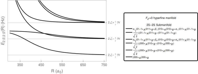
Figure 7: Energy levels of the $2S$–$2S$ states within the $F_{z}=0$ hyperfine manifold as a function of atomic separation $R$ (given in units of the Bohr radius $a_{0}$). The eigenstates in the legend are those relevant to the $R\to\infty$ asymptotic limit; for finite separation these states mix. There is one remaining level crossing even if the Hamiltonian matrix is irreducible. The coefficients $\alpha_{\pm}$ and $\beta_{\pm}$ are determined from second-order perturbation theory and given by Eq. (41). The states are labeled from top to bottom in the legend, in the same order as they are relevant to the long-range asymptotics.

The adjacency matrix $U_{F_{z}=0}$ of the Hamiltonian (17) in the $F_{Z}=0$ manifold is equal to

$$\left(\begin{array}[]{cccccccccccccccccccccccc}1&0&0&0&0&0&0&0&0&0&0&0&0&0&0&0&0&1&0&0&0&1&0&1\\ 0&1&0&0&0&0&0&0&0&0&0&0&0&0&0&0&0&1&0&0&1&0&0&1\\ 0&0&1&0&0&0&0&0&0&0&0&0&0&0&0&0&1&0&0&1&0&0&1&0\\ 0&0&0&1&0&0&0&0&0&0&0&0&0&0&0&0&1&0&1&0&0&0&1&0\\ 0&0&0&0&1&0&0&0&0&0&0&0&0&0&1&1&0&1&0&0&1&1&0&0\\ 0&0&0&0&0&1&0&0&0&0&0&0&1&1&0&0&1&0&1&1&0&0&0&0\\ 0&0&0&0&0&0&1&0&0&0&0&0&0&0&0&1&0&1&0&0&0&0&0&1\\ 0&0&0&0&0&0&0&1&0&0&0&0&0&0&1&0&0&1&0&0&0&0&0&1\\ 0&0&0&0&0&0&0&0&1&0&0&0&0&1&0&0&1&0&0&0&0&0&1&0\\ 0&0&0&0&0&0&0&0&0&1&0&0&1&0&0&0&1&0&0&0&0&0&1&0\\ 0&0&0&0&0&0&0&0&0&0&1&0&0&0&1&1&0&0&0&0&1&1&0&1\\ 0&0&0&0&0&0&0&0&0&0&0&1&1&1&0&0&0&0&1&1&0&0&1&0\\ 0&0&0&0&0&1&0&0&0&1&0&1&1&0&0&0&0&0&0&0&0&0&0&0\\ 0&0&0&0&0&1&0&0&1&0&0&1&0&1&0&0&0&0&0&0&0&0&0&0\\ 0&0&0&0&1&0&0&1&0&0&1&0&0&0&1&0&0&0&0&0&0&0&0&0\\ 0&0&0&0&1&0&1&0&0&0&1&0&0&0&0&1&0&0&0&0&0&0&0&0\\ 0&0&1&1&0&1&0&0&1&1&0&0&0&0&0&0&1&0&0&0&0&0&0&0\\ 1&1&0&0&1&0&1&1&0&0&0&0&0&0&0&0&0&1&0&0&0&0&0&0\\ 0&0&0&1&0&1&0&0&0&0&0&1&0&0&0&0&0&0&1&0&0&0&0&0\\ 0&0&1&0&0&1&0&0&0&0&0&1&0&0&0&0&0&0&0&1&0&0&0&0\\ 0&1&0&0&1&0&0&0&0&0&1&0&0&0&0&0&0&0&0&0&1&0&0&0\\ 1&0&0&0&1&0&0&0&0&0&1&0&0&0&0&0&0&0&0&0&0&1&0&0\\ 0&0&1&1&0&0&0&0&1&1&0&1&0&0&0&0&0&0&0&0&0&0&1&0\\ 1&1&0&0&0&0&1&1&0&0&1&0&0&0&0&0&0&0&0&0&0&0&0&1\\ \end{array}\right)\,.$$ (24)

The accumulated adjacency matrix has the structure

$$A_{F_{z}=0}=\sum_{i=1}^{24}U^{i}\simeq\left(\begin{array}[]{cccccccccccccccccccccccc}\chi&\chi&0&0&\chi&0&\chi&\chi&0&0&\chi&0&0&0&\chi&\chi&0&\chi&0&0&\chi&\chi&0&\chi\\ \chi&\chi&0&0&\chi&0&\chi&\chi&0&0&\chi&0&0&0&\chi&\chi&0&\chi&0&0&\chi&\chi&0&\chi\\ 0&0&\chi&\chi&0&\chi&0&0&\chi&\chi&0&\chi&\chi&\chi&0&0&\chi&0&\chi&\chi&0&0&\chi&0\\ 0&0&\chi&\chi&0&\chi&0&0&\chi&\chi&0&\chi&\chi&\chi&0&0&\chi&0&\chi&\chi&0&0&\chi&0\\ \chi&\chi&0&0&\chi&0&\chi&\chi&0&0&\chi&0&0&0&\chi&\chi&0&\chi&0&0&\chi&\chi&0&\chi\\ 0&0&\chi&\chi&0&\chi&0&0&\chi&\chi&0&\chi&\chi&\chi&0&0&\chi&0&\chi&\chi&0&0&\chi&0\\ \chi&\chi&0&0&\chi&0&\chi&\chi&0&0&\chi&0&0&0&\chi&\chi&0&\chi&0&0&\chi&\chi&0&\chi\\ \chi&\chi&0&0&\chi&0&\chi&\chi&0&0&\chi&0&0&0&\chi&\chi&0&\chi&0&0&\chi&\chi&0&\chi\\ 0&0&\chi&\chi&0&\chi&0&0&\chi&\chi&0&\chi&\chi&\chi&0&0&\chi&0&\chi&\chi&0&0&\chi&0\\ 0&0&\chi&\chi&0&\chi&0&0&\chi&\chi&0&\chi&\chi&\chi&0&0&\chi&0&\chi&\chi&0&0&\chi&0\\ \chi&\chi&0&0&\chi&0&\chi&\chi&0&0&\chi&0&0&0&\chi&\chi&0&\chi&0&0&\chi&\chi&0&\chi\\ 0&0&\chi&\chi&0&\chi&0&0&\chi&\chi&0&\chi&\chi&\chi&0&0&\chi&0&\chi&\chi&0&0&\chi&0\\ 0&0&\chi&\chi&0&\chi&0&0&\chi&\chi&0&\chi&\chi&\chi&0&0&\chi&0&\chi&\chi&0&0&\chi&0\\ 0&0&\chi&\chi&0&\chi&0&0&\chi&\chi&0&\chi&\chi&\chi&0&0&\chi&0&\chi&\chi&0&0&\chi&0\\ \chi&\chi&0&0&\chi&0&\chi&\chi&0&0&\chi&0&0&0&\chi&\chi&0&\chi&0&0&\chi&\chi&0&\chi\\ \chi&\chi&0&0&\chi&0&\chi&\chi&0&0&\chi&0&0&0&\chi&\chi&0&\chi&0&0&\chi&\chi&0&\chi\\ 0&0&\chi&\chi&0&\chi&0&0&\chi&\chi&0&\chi&\chi&\chi&0&0&\chi&0&\chi&\chi&0&0&\chi&0\\ \chi&\chi&0&0&\chi&0&\chi&\chi&0&0&\chi&0&0&0&\chi&\chi&0&\chi&0&0&\chi&\chi&0&\chi\\ 0&0&\chi&\chi&0&\chi&0&0&\chi&\chi&0&\chi&\chi&\chi&0&0&\chi&0&\chi&\chi&0&0&\chi&0\\ 0&0&\chi&\chi&0&\chi&0&0&\chi&\chi&0&\chi&\chi&\chi&0&0&\chi&0&\chi&\chi&0&0&\chi&0\\ \chi&\chi&0&0&\chi&0&\chi&\chi&0&0&\chi&0&0&0&\chi&\chi&0&\chi&0&0&\chi&\chi&0&\chi\\ \chi&\chi&0&0&\chi&0&\chi&\chi&0&0&\chi&0&0&0&\chi&\chi&0&\chi&0&0&\chi&\chi&0&\chi\\ 0&0&\chi&\chi&0&\chi&0&0&\chi&\chi&0&\chi&\chi&\chi&0&0&\chi&0&\chi&\chi&0&0&\chi&0\\ \chi&\chi&0&0&\chi&0&\chi&\chi&0&0&\chi&0&0&0&\chi&\chi&0&\chi&0&0&\chi&\chi&0&\chi\\ \end{array}\right)\,,$$ (25)

where $\chi$ stands for any entry different from zero (the $\chi$s are not all equal). The adjacency graph given in Fig. 6 confirms the presence of two irreducible submatrices of $H_{F_{z}=0}$. Indeed, the two uncoupled subspaces are spanned by the states $|\Psi_{i}\rangle$ with $i=1,2,5,7,8,11,15,16,18,21,22,24$ (subspace I), and $|\Psi_{j}\rangle$ with $j=3,4,6,9,10,12,13,14,17,19,20,23$ (subspace II). An ordering of the eigenvalues reveals that one can have coupling among the $S$–$S$ and $P$–$P$ states (distributed among atoms $A$ and $B$), forming submanifold I, and among all $S$–$P$ and $P$–$S$ states (distributed among atoms $A$ and $B$), forming submanifold II. In retrospect, the separation is perhaps clear, but it is less obvious at first glance.

It is then possible to redefine the levels from which the $12\times 12$ Hamiltonian matrix is constructed, in the first submanifold of $F_{z}=0$ (the $S$–$S$ coupled states). Specifically, one defines $|\Psi_{1}^{\left(\mathrm{\@slowromancap i@}\right)}\rangle=|\Psi_{1}\rangle$, $|\Psi_{2}^{\left(\mathrm{\@slowromancap i@}\right)}\rangle=|\Psi_{2}\rangle$, $|\Psi_{3}^{\left(\mathrm{\@slowromancap i@}\right)}\rangle=|\Psi_{5}\rangle$, $|\Psi_{4}^{\left(\mathrm{\@slowromancap i@}\right)}\rangle=|\Psi_{7}\rangle$, $|\Psi_{5}^{\left(\mathrm{\@slowromancap i@}\right)}\rangle=|\Psi_{8}\rangle$, $|\Psi_{6}^{\left(\mathrm{\@slowromancap i@}\right)}\rangle=|\Psi_{11}\rangle$, $|\Psi_{7}^{\left(\mathrm{\@slowromancap i@}\right)}\rangle=|\Psi_{15}\rangle$, $|\Psi_{8}^{\left(\mathrm{\@slowromancap i@}\right)}\rangle=|\Psi_{16}\rangle$, $|\Psi_{9}^{\left(\mathrm{\@slowromancap i@}\right)}\rangle=|\Psi_{18}\rangle$, $|\Psi_{10}^{\left(\mathrm{\@slowromancap i@}\right)}\rangle=|\Psi_{21}\rangle$, $|\Psi_{11}^{\left(\mathrm{\@slowromancap i@}\right)}\rangle=|\Psi_{22}\rangle$, and $|\Psi_{12}^{\left(\mathrm{\@slowromancap i@}\right)}\rangle=|\Psi_{24}\rangle$. Within the space spanned by the $|\Psi_{i}^{\left(\mathrm{\@slowromancap i@}\right)}\rangle$ with $i=1,2,\dots,12$, the Hamiltonian matrix has the structure

$$H_{F_{z}=0}^{\left(\mathrm{\@slowromancap i@}\right)}= \;\left(\begin{array}[]{cccccccccccc}2{\mathcal{L}}-\tfrac{9}{2}{\mathcal{H}}&0&0&0&0&0&0&0&-{\mathcal{V}}&0&-2{\mathcal{V}}&-{\mathcal{V}}\\ 0&2{\mathcal{L}}-\tfrac{3}{2}{\mathcal{H}}&0&0&0&0&0&0&{\mathcal{V}}&-2{\mathcal{V}}&0&-{\mathcal{V}}\\ 0&0&2{\mathcal{L}}+\tfrac{3}{2}{\mathcal{H}}&0&0&0&-{\mathcal{V}}&{\mathcal{V}}&2{\mathcal{V}}&-{\mathcal{V}}&{\mathcal{V}}&0\\ 0&0&0&2{\mathcal{L}}-\tfrac{3}{2}{\mathcal{H}}&0&0&0&-2{\mathcal{V}}&-{\mathcal{V}}&0&0&{\mathcal{V}}\\ 0&0&0&0&2{\mathcal{L}}+\tfrac{3}{2}{\mathcal{H}}&0&-2{\mathcal{V}}&0&{\mathcal{V}}&0&0&{\mathcal{V}}\\ 0&0&0&0&0&2{\mathcal{L}}+\tfrac{3}{2}{\mathcal{H}}&-{\mathcal{V}}&-{\mathcal{V}}&0&{\mathcal{V}}&{\mathcal{V}}&2{\mathcal{V}}\\ 0&0&-{\mathcal{V}}&0&-2{\mathcal{V}}&-{\mathcal{V}}&-\tfrac{3}{2}{\mathcal{H}}&0&0&0&0&0\\ 0&0&{\mathcal{V}}&-2{\mathcal{V}}&0&-{\mathcal{V}}&0&-\tfrac{1}{2}{\mathcal{H}}&0&0&0&0\\ -{\mathcal{V}}&{\mathcal{V}}&2{\mathcal{V}}&-{\mathcal{V}}&{\mathcal{V}}&0&0&0&\tfrac{1}{2}{\mathcal{H}}&0&0&0\\ 0&-2{\mathcal{V}}&-{\mathcal{V}}&0&0&{\mathcal{V}}&0&0&0&-\tfrac{1}{2}{\mathcal{H}}&0&0\\ -2{\mathcal{V}}&0&{\mathcal{V}}&0&0&{\mathcal{V}}&0&0&0&0&\tfrac{1}{2}{\mathcal{H}}&0\\ -{\mathcal{V}}&-{\mathcal{V}}&0&{\mathcal{V}}&{\mathcal{V}}&2{\mathcal{V}}&0&0&0&0&0&\tfrac{1}{2}{\mathcal{H}}\end{array}\right)\,,$$ (38)

where

$$\mathcal{V}=3\,\alpha\,\hbar c\,\frac{a_{0}^{2}}{R^{3}}\$$ (39)

is a parameter that describes the strength of the van der Waals interaction. Furthermore,

$${\mathcal{H}}=\frac{\alpha^{4}}{18}\,g_{N}\,\frac{m}{m_{p}}\,m\,c^{2}$$ (40)

with ${\mathcal{H}}\approx h\times 59.1856114(22)\,{\rm MHz}$, parameterizes the hyperfine splitting ($m_{p}$ is the proton mass). A close-up of the six energetically highest, distance-dependent $S$–$S$ state energy levels, coupled through virtual $P$–$P$ states, is given in Fig. 7 (Born-Oppenheimer potential energy curves). We have verified that the crossing between the second and third level (counted in ascending order of the unperturbed energy for $R\to\infty$) persists under a drastic increase of the numerical accuracy, much like for our model problem (Fig. 3). The coefficients used in the legend for this figure are given by

$$\alpha_{\pm} =2\sqrt{\frac{2}{33\pm\sqrt{33}}}\,,$$ (41a)

$$\beta_{\pm} =\mp\frac{\sqrt{33}\pm 1}{\sqrt{2\left(33\pm\sqrt{33}\right)}}\,.$$ (41b)

Despite the fact that subspace I is irreducible, one observes one level crossing, much in line with the discussion presented in Sec. II. Finer details of the calculation will be presented in an upcoming work Jentschura et al. (2016). Specifically, for large $R$, we can point out that all of the level shifts of the states in Fig. 7 are found to be of order $\mathcal{V}^{2}/\mathcal{L}$ and are thus of second order in ${\mathcal{V}}$, proportional to $1/R^{6}$ but drastically enhanced in their numerical magnitude as compared to “normal” van der Waals shifts due to the $1/{\mathcal{L}}$ denominator. For the $1S$–$1S$ interaction, the well-known result involves a shift of order $\mathcal{V}^{2}/E_{h}$, where $E_{h}$ is the Hartree energy. In the limit of large $R$, the $2S$–$2S$ interaction is seen to be larger by a factor $1/\alpha^{3}\sim 10^{6}$, in view of the smaller energy denominator which only involves the Lamb shift.

V Conclusions

Often, in physics, we need to resort to mathematical sophistications in order to uncover properties of a physical system hidden from us at first glance. In our case, we find that adjacency matrices and adjacency graphs help determine the reducibility of a matrix, and, in the analysis of the hyperfine-resolved $2S$–$2S$ interaction, help determine the irreducible subspaces into which we may break the total Hamiltonian. We were able to identify an additional selection rule, which is relatively obvious a posteriori, namely, that couplings occur between $S$–$S$ and $P$–$P$ levels, and between $S$–$P$ and $P$–$S$ levels, but there are no coupling joining the two submanifolds (see Sec. IV). The size of the matrix is reduced from $24\times 24$ to $12\times 12$. It is somewhat surprising that the seemingly easy problem of identifying the irreducible submatrices of a Hamiltonian, involves a rather sophisticated concept like an adjacency matrix.

Our model problem, studied in Sec. II and III, reveals that level crossings can occur even in well-behaved quantum mechanical systems, described by inter-level couplings varying with some parameter. For the long-range interaction between atoms, the inverse interatomic distance $1/R$ is such a coupling parameter. In Fig. 2 (model problem), and in Fig. 7 ($2S$–$2S$ states within the $F_{z}=0$ submanifold of the hydrogen long-range interaction), level crossings are clearly visible even if the Hamiltonian matrix is irreducible. Our extended-precision numerical calculations (Fig. 3) and the analytic structure of the “crossing” eigenvectors in Eq. (11) together with the adjacency matrices in Figs. 4 and 5 indicate that the no-crossing theorem breaks down in higher-dimensional systems. Furthermore, we observe that our crossings, both for the model problem as well as for the $2S$–$2S$ system, involve situations where the couplings are indirect and the admixtures at the crossing point are between levels which are displaced from each other in the adjacency graph by at least two elementary steps. These observations could be of interest beyond the the concrete problem studied here, in the context of a breakdown of the no-crossing theorem in higher-dimensional quantum mechanical systems. An improved understanding of the 2S–2S interaction is important for progress in the 2S hyperfine measurement by optical methods, using an atomic beam Fischer et al. (2002); Kolachevsky et al. (2004, 2009).

Attempts to study the hyperfine-resolved interaction have been made, but no reference has been made to the resolution of the hyperfine structure Jonsell et al. (2002); Simonsen et al. (2011). The current approach leads to a solution, with partial results being presented in Eq. (38) and Fig. 7 and finer details being relegated to Ref. Jentschura et al. (2016).

References

Cohen-Tannoudji et al. (1978a)C. Cohen-Tannoudji, B. Diu, and F. Lalo, Quantum
Mechanics (Volume 1), 1st ed. (J. Wiley & Sons, New York, 1978).
Cohen-Tannoudji et al. (1978b)C. Cohen-Tannoudji, B. Diu, and F. Lalo, Quantum
Mechanics (Volume 2), 1st ed. (J. Wiley & Sons, New York, 1978).
Jentschura et al. (2016)U. D. Jentschura, V. Debierre, C. M. Adhikari, A. Matveev, and N. Kolachevsky, Long-range interactions of
excited hydrogen atoms. II. Hyperfine-resolved -system, submitted
to Physical Review A (2016).
Wolfram (1999)S. Wolfram, The Mathematica
Book, 4th ed. (Cambridge
University Press, Cambridge, UK, 1999).
(5)See the URL
http://en.m.wikipedia.org/wiki/Avoided_crossing.
Landau and Lifshitz (1958)L. D. Landau and E. M. Lifshitz, Quantum
Mechanics, Volume 3 of the Course on Theoretical Physics (Pergamon Press, Oxford, UK, 1958).
Jonsell et al. (2002)S. Jonsell, A. Saenz,
P. Froelich, R. C. Forrey, R. Côté, and A. Dalgarno, “Long-range interactions between two 2s excited
hydrogen atoms,” Phys. Rev. A 65, 042501
(2002).
Simonsen et al. (2011)S. I. Simonsen, L. Kocbach, and J. P. Hansen, “Long-range
interactions and state characteristics of interacting Rydberg atoms,” J. Phys. B 44, 165001 (2011).
Itzykson and Zuber (1980)C. Itzykson and J. B. Zuber, Quantum Field
Theory (McGraw-Hill, New
York, 1980).
Lundeen and Pipkin (1981)S. R. Lundeen and F. M. Pipkin, “Measurement of the Lamb Shift in Hydrogen, ,” Phys. Rev. Lett. 46, 232–235 (1981).
Fischer et al. (2002)M. Fischer, N. Kolachevsky, S. G. Karshenboim, and T. W. Hänsch, “Optical measurement of the 2S hyperfine interval in atomic
hydrogen,” Can.
J. Phys. 80, 1225–1231
(2002).
Kolachevsky et al. (2004)N. Kolachevsky, M. Fischer, S. G. Karshenboim, and T. W. Hänsch, “High-Precision Optical Measurement of the Hyperfine Interval in
Atomic Hydrogen,” Phys. Rev. Lett. 92, 033003 (2004).
Kolachevsky et al. (2009)N. Kolachevsky, A. Matveev, J. Alnis,
C. G. Parthey, S. G. Karshenboim, and T. W. Hänsch, “Measurement of the Hyperfine
Interval in Atomic Hydrogen,” Phys. Rev. Lett. 102, 213002 (2009).