Null weak values and the past of a quantum particle

Abstract

Non-destructive weak measurements (WM) made on a quantum particle allow to extract information as the particle evolves from a prepared state to a finally detected state. The physical meaning of this information has been open to debate, particularly in view of the apparent discontinuous trajectories of the particle recorded by WM. In this work we investigate the properties of vanishing weak values for projection operators as well as general observables. We then analyze the implications when inferring the past of a quantum particle. We provide a novel (non-optical) example for which apparent discontinuous trajectories are obtained by WM. Our approach is compared to previous results.

I Introduction

Assume a quantum system is prepared in some initial state at time $t_{i}$, and ultimately detected and found to be in some final state at time $t_{f}$. It is usually taken for granted that quantum mechanics does not allow to learn anything concerning the property of the system at some intermediate time. The reason is that in order to learn something about a given property, the associated observable needs to be measured. But as is well-known, measurements are special in quantum mechanics: measurements break the unitary evolution and project the premeasurement system state to one of the eigenstates of the measured observable. Hence in typical cases a measurement made at some intermediate time will irremediably disturb the system evolution from what it would have been without this intermediate measurement. The upshot is that it is impossible to ascertain the particle’s properties, and in particular its past when the system has evolved from a given initial state to a final state. The best we can do is employ counterfactual reasoning, but Bohr has long ago warned us bohr-einsteinbook that this would lead to paradoxes, as exemplified in the well-known Delayed Choice Experiment proposed by Wheeler wheeler-delayed .

However there have been recent proposals to ascertain the paths taken by a quantum particle. In particular Vaidman examined the path of a photon in nested interferometers vaidman2013 , while one of us investigated the dynamical paths compatible with a given final state when a quantum system evolution is generated by a semiclassical Feynman propagator A2012PRL . These proposals are based on weak measurements. Weak measurements were introduced AAV in 1988 as a theoretical scheme for minimally perturbing non-destructive quantum measurements. Aharonov, Albert and Vaidman precisely showed AAV that, without departing from the standard quantum formalism, it was possible to measure an observable $A$ in a particular sense without appreciably changing the system evolution. The main idea is to achieve an interaction with a weak coupling between $A$ and a dynamical variable of an external degree of freedom (an ancilla that will be called “quantum pointer”). The system and the quantum pointer are entangled, until the final projective measurement of a different system observable $B$ correlates the obtained system eigenstate with the quantum state of the weak pointer. The state of the weak pointer has picked up a shift (relative to its initial state) proportional to a quantity known as the weak value of $A$. When a weak value vanishes, the state of the quantum pointer remains unchanged, and Refs vaidman2013 ; A2012PRL interpreted this fact by asserting that the system property coupled to the pointer was not there (otherwise the pointer state would have changed).

While many experimental and theoretical works dealing with weak measurements have been published in the last decade (see RMP for a review) the meaning of the observed weak values has been debated since their inception, from the early comments by Leggett leggett89 and Peres peresWM to more recent works sokolovski16 ; svensson2014 . Unsurprisingly, any proposal to infer the past of a quantum system from the weak values is going to face criticism disputing the relevance of weak measurements concerning the properties that can be ascribed to a system during its evolution. In particular, Vaidman vaidman2013 ; A2012PRL noted that the weak values of the spatial projector were non-zero inside a Mach-Zehnder interferometer (MZI) inserted on one of the arms of another larger Mach-Zehnder, but the weak values along that arm did vanish before and beyond the nested MZI. The same feature was also remarked A2013JPA in a 3 path interferometer: when 2 of the 3 branches are joined, the spatial projector weak value (that did not vanish on either of these 2 arms) vanishes once these 2 branches merge. If a non-vanishing weak value is interpreted as a trace left by a particle, while a vanishing weak value implies the particle wasn’t there, one would be led to conclude for instance that the particle was inside the nested MZI while it could never have entered or exited, a rather strange conclusion.

Indeed, several authors zubairy2013 ; vaidman-com2013 ; saldanha2014 ; bartkiewicz2015 ; ferenczi2015 ; jordan-dove ; sokolovskiMZI2016 ; griffiths2016 ; bula2016 ; vaidman-com2016 have criticised such an idea, generally basing their critcism on the experimental realization danan2013 of Vaidman’s nested MZI proposal. Some of the criticism zubairy2013 ; saldanha2014 ; ferenczi2015 ; bula2016 is essentially relevant to the details of the experiment (that employed tilting mirrors and classical electromagnetic waves). In this paper we will instead be concerned by fundamental issues concerning the properties of a quantum system between preparation and detection. Indeed, relying on a classical optics experiment, or even on quantum optics, in order to interpret a quantity derived in the context of non-relativistic quantum mechanics requires at best an amount of extrapolation that will not help in giving a solid account of the meaning of null weak values. This is precisely the aim of the present work: to analyze and understand null weak values, and from there examine which interpretations can make sense. To the best of our knowledge, such a work has not been undertaken.

This work is organized as follows. We will first recall the weak measurements formalism (Sec. II). We will then carefully scrutinize the case of vanishing weak values and give a couple of illustrations (Sec. III). Sec. IV will be devoted to the interpretation of null weak values, and we will discuss and compare with the views expounded in the recent papers vaidman2013 ; saldanha2014 ; vaidman-past ; jordan-dove ; sokolovskiMZI2016 ; griffiths2016 . We will draw our conclusions in Sec. V.

II Weak Measurements

The underlying idea at the basis of the weak measurement (WM) framework is to give an answer the question:“what is the value of a property (represented by an observable $A$) of a quantum system while it is evolving from an initial state $\mathit{\left|\psi(t_{i})\right\rangle}$ to a final state $\left|\chi(t_{f})\right\rangle$ obtained as a result of an usual projective measurement?”. As our interest in this paper concerns the instance of null weak values, we will restrict our exposition to the simplest case, a bivalued observable $A$, with eigenstates and eigenvalues denoted by $A\left|a_{k}\right\rangle=a_{k}\left|a_{k}\right\rangle,$ $k=1,2$.

Let us assume that at $t=t_{i}$ the system of interest is prepared into the state $\left|\psi(t_{i})\right\rangle$ (this step is known as preselection). An ancilla (that will play the role of a quantum pointer) is at that time in state $\left|\varphi(t_{i})\right\rangle,$ so the total initial quantum state is the uncoupled state

$$\left|\Psi(t_{i})\right\rangle=\left|\psi(t_{i})\right\rangle\left|\varphi(t_{i})\right\rangle.$$ (1)

We assume the system and the pointer will interact during a brief time interval $\tau$ centered around $t=t_{w}$ (physically corresponding to the time during which the system and the quantum pointer interact). Let the interaction Hamiltonian be specified by

$$H_{int}=g(t)AP$$ (2)

coupling the system observable ${A}$ to the momentum $P$ of the pointer. $g(t)$ is a smooth function non-vanishing only in the interval $t_{w}-\tau/2<t<t_{w}+\tau/2$ and such that $g\equiv\int_{t_{w}-\tau/2}^{t_{w}+\tau/2}g(t)dt$ appears as the effective coupling constant. Eq. (2) is nothing but the usual interaction employed to account for projective measurements of $A$ : in that case $g(t)$ is a sharply peaked function correlating each $\left|a_{k}\right\rangle$ to an orthogonal state of a macroscopic pointer, that collapses projecting the system state to a random eigenstate $\left|a_{k_{0}}\right\rangle$. Here instead $g(t)$ will be small, the pointer is quantum, and the pointer-system will evolve unitarily until a subsequent projective measurement made on the system will correlate the quantum pointer to a specific final state of the system, as we now detail.

Let us denote by $U(t_{w},t_{i})$ the system evolution operator between $t_{i}$ and $t_{w}$ and disregard the self-evolution of the pointer state. After the interaction $(t>t_{w}+\tau/2)$ the initial uncoupled state (1) has become entangled:

$$\left|\Psi(t)\right\rangle =U(t,t_{w})e^{-ig{A}P}U(t_{w},t_{i})\left|\psi(t_{i})\right\rangle\left|\varphi(t_{i})\right\rangle$$ (3)

$$=U(t,t_{w})e^{-ig{A}P}\left|\psi(t_{w})\right\rangle\left|\varphi(t_{i})\right\rangle$$ (4)

$$=U(t,t_{w})\sum_{k=1,2}e^{-iga_{k}P}\left\langle a_{k}\right|\left.\psi(t_{w})\right\rangle\left|a_{k}\right\rangle\left|\varphi(t_{i})\right\rangle.$$ (5)

Finally, the system undergoes a standard projective measurement at time $t_{f}:$ an observable $B$ (different from $A$) is measured and the system ends up in one of its eigenstates $\left|b_{k}\right\rangle$. Let us only keep the results corresponding to a chosen eigenvalue $b_{k_{0}}$ and label the postselected state by $\left|\chi(t_{f})\right\rangle\equiv\left|b_{k_{0}}\right\rangle$. The projection on the entangled state $\left|\Psi(t_{f})\right\rangle$ given by Eq. (5) leads to the final state of the pointer correlated with the postselected system state:

$$\left|\varphi(t_{f})\right\rangle=\sum_{k=1,2}\left[\left\langle\chi(t_{w})\right|\left.a_{k}\right\rangle\left\langle a_{k}\right|\left.\psi(t_{w})\right\rangle\right]e^{-iga_{k}P}\left|\varphi(t_{i})\right\rangle.$$ (6)

If $\left|\varphi(t_{i})\right\rangle$ is a localized state in the position representation, then $\varphi(x,t_{f})$ is given by a superposition of shifted initial states

$$\varphi(x,t_{f})=\sum_{k=1,2}\left[\left\langle\chi(t_{w})\right|\left.a_{k}\right\rangle\left\langle a_{k}\right|\left.\psi(t_{w})\right\rangle\right]\varphi(x+ga_{k},t_{i}).$$ (7)

This expression is the first step of the usual von Neumann projective by which each eigenstate $\left|a_{k}\right\rangle$ of the measured observable is correlated with a given state $\varphi(x+ga_{k})$ of the pointer (but in a von Neumann measurement the second step is a projection to an eigenstate $\left|a_{k_{f}}\right\rangle$ of A, which does not happen here).

Let us now assume the coupling $g$ is sufficiently small so that $e^{-iga_{k}P}\approx 1-iga_{k}P$ holds for each $k$. Eq. (6) becomes

$$\left|\varphi(t_{f})\right\rangle =\left\langle\chi(t_{w})\right|\left.\psi(t_{w})\right\rangle\left(1-igP\frac{\left\langle\chi(t_{w})\right|{A}\left|\psi(t_{w})\right\rangle}{\left\langle\chi(t_{w})\right|\left.\psi(t_{w})\right\rangle}\right)\left|\varphi(t_{i})\right\rangle$$ (8)

$$=\left\langle\chi(t_{w})\right|\left.\psi(t_{w})\right\rangle\exp\left(-igA^{w}P\right)\left|\varphi(t_{i})\right\rangle$$ (9)

where

$$A^{w}=\frac{\left\langle\chi(t_{w})\right|A\left|\psi(t_{w})\right\rangle}{\left\langle\chi(t_{w})\right|\left.\psi(t_{w})\right\rangle}$$ (10)

is the weak value of the observable $A$ given pre and postselected states $\left|\psi\right\rangle$ and $\left|\chi\right\rangle$ respectively (we will sometimes employ instead the full notation $A_{\left\langle\chi\right|,\left|\psi\right\rangle}^{w}$ to specify pre and postselection). For a localized pointer state, expanding to first order the terms $\varphi(x+ga_{k},t_{i})$ in Eq. (7) leads to Eq. (9): the overall shift $\varphi(x+gA_{w},t_{i})$ is readily seen to result from the interference due to the superposition of the slightly shifted terms $\varphi(x+ga_{k},t_{i})$.

We can now summarize the weak measurement protocol: (i) preselection, ie preparation of the initial state (1); (ii) weak coupling through the measurement Hamiltonian (2); (iii) postselection, leading to the quantum state of the pointer (9); (iv) readout (measurement) of the quantum pointer. The quantum pointer readout allows to extract the weak value: Eq. (9) indicates that the pointer will undergo a translation proportional to the weak value.

III Null Weak Values

III.1 Weak values: general properties

Following Eqs. (7)-(9) the real part of the weak value $A_{w}$ appears as the shift brought to the average initial pointer state position $\varphi(x,t_{i})$ due to its coupling with the system via the local interaction Hamitonian (2). The weak values are generally different from the eigenvalues. Indeed, the weak coupling step correlates the system observable eigenstates with pointer states, but a single eigenstate is only obtained for strong couplings (relative to the pointer states spread), and that a random projection takes place. The system’s state is thus radically modified when undergoing a transition from its pre-measurement state to an eigenstate. The eigenvalue associated to this observable eigenstate reflects the value taken by the corresponding property after this radical change of state.

Instead, the system-pointer coupling in a weak measurement practically leaves the system state unaffected: since

$$e^{-ig{A}P}\left|\psi(t_{w})\right\rangle\left|\varphi(t_{i})\right\rangle\approx\left|\psi(t_{w})\right\rangle\left|\varphi(t_{i})\right\rangle-iA\left(g\left|\psi(t_{w})\right\rangle\right)P\left|\varphi(t_{i})\right\rangle$$ (11)

The tiny fraction $g\left|\psi(t_{w})\right\rangle$ of the system state that interacts is precisely the one that couples to the quantum pointer. The weak value appears as the imprint of this coupling left on the pointer, conditioned on the final projective measurement (postselection). The weak value as defined from Eq. (10) can be seen as the ratio of the transition amplitude to the final state $\left|\chi(t_{w})\right\rangle$ of the fraction of the state $A\left|\psi(t_{w})\right\rangle$ that has interacted relative to a non-interaction situation in which the system state remains $\left|\psi(t_{w})\right\rangle$. In particular the numerator is the standard transition amplitude matrix element for the observable $A.$ Hence a weak value cannot be associated with an eigenstate but with a transition from a preselected to a postselected state. Nevertheless, weak values obey a similar relation with regard to the computation of expectation values: the standard expectation value of $A$ in state $\left|\psi(t_{w})\right\rangle$ is given in terms of eigenvalues by the textbook expression

$$\left\langle\psi(t_{w})\right|{A}\left|\psi(t_{w})\right\rangle=\sum_{f}\left|\left\langle a_{f}\right|\left.\psi(t_{w})\right\rangle\right|^{2}a_{f}.$$ (12)

It can also be written in terms of weak values as

$$\left\langle\psi(t_{w})\right|A\left|\psi(t_{w})\right\rangle=\sum_{f}\left|\left\langle\chi_{f}(t_{f})\right|\left.\psi(t_{f})\right\rangle\right|^{2}A_{\left\langle\chi_{f}\right|,\left|\psi\right\rangle}^{w}$$ (13)

with $\left|\chi_{f}(t_{f})\right\rangle=\left|b_{f}\right\rangle.$ Rather than involving the probability of obtaining an eigenstate, Eq. (13) is expressed in terms of the probabilities of obtaining a postselected state $\left|b_{f}\right\rangle.$ Then the weak value indicated by the quantum pointer that was coupled to $A$ replaces the eigenvalue in the usual expression (12). Note that the imaginary part of the right handside of Eq. (13) is zero.

III.2 Null weak values

III.2.1 Vanishing eigenvalues

Let us first examine the case of vanishing eigenvalues. In the standard von Neumann measurement scheme, a null eigenvalue implies that the (macroscopic) pointer state is left untouched: the coupling has no effect on the pointer. But apart from this specificity, a vanishing eigenvalue appears as the result of a standard projective measurement: the system state changes, as it is projected to the eigenstate associated with the null eigenvalue for the measured observable. For example imagine a particle entering a Mach-Zehnder interferometer. After the beamsplitter, its quantum state of each atom can be described by the superposition $\left|I\right\rangle+\left|II\right\rangle$, where $\left|I\right\rangle$ ($\left|II\right\rangle$) denotes the wavepackets traveling along arm $I$ ($II\text{)}$. If a standard measurement of the projector onto path $\Pi_{I}\equiv\left|I\right\rangle\left\langle I\right|$ yields 0, then (i) the particle is not on path $I$ and (ii) its quantum state has collapsed to $\left|II\right\rangle$ (one is certain to find the particle on that path).

As another example, consider a particle with integer spin. Then measuring the spin projection along some direction can yield a null eigenvalue. The spin state is then projected to the corresponding eigenstate (as can be verified by making subsequent measurements) corresponding to no spin component along that direction. Hence we can assert that when a vanishing eigenvalue is obtained, the initial system state has been radically perturbed (as per any projective measurement) but the pointer state has remained the same because the property that has been measured is not there (no particle, no spin component).

III.2.2 Transition amplitudes

As seen above, for weak measurements the system’s state is not projected after the weak coupling. Hence a null weak value leaves the pointer untouched (the coupling has no effect) just as in the case of null eigenvalues, but the implication does not concern eigenvectors but transitions to the postselected state. This follows from the weak values definition (10): $A^{w}=0$ iff $\left\langle\chi(t_{w})\right|A\left|\psi(t_{w})\right\rangle=0$, so a vanishing weak value is obtained when the transition between the fraction of the state that has interacted $A\left|\psi(t_{w})\right\rangle$ and the postselected state is forbidden. As explained in Sec. II, if the evolution of the states between the initial, interaction and postselection times is not trivial, then the vanishing transition is between the state at the time the weak coupling takes place (with the preselected state forwarded in time) and the postselected state evolved backward in time, or alternatively with the transformed state $A\left|\psi(t_{w})\right\rangle$ evolved up to $t_{f}$ and the postselected state.

As is well known from elementary quantum mechanics, a forbidden transition means that the final state cannot be reached under the action of the observable operator on the initial state. Here the final state is the postselected state, and the action of the operator transforming the pre-measurement state is physically due to the weak interaction between the system and the quantum pointer. Under this setting, weak measurements can be seen as an experimentally feasible protocol in order to measure the vanishing transition amplitudes.

III.2.3 Meaning of null weak values

A null weak value correlates successful postselection with the quantum pointer having been left unchanged despite the interaction with the system. The reason, as seen in the preceding paragraph, is that the transition amplitude vanishes. If the postselected state is obtained, then the property represented by $A$ cannot be detected by the weakly coupled quantum pointer. For example when the weak value $\Pi_{I}^{w}$ of a spatial projector $\Pi_{I}\equiv\left|I\right\rangle\left\langle I\right|$ vanishes this means that the postselected state cannot be reached from the region $\left|I\right\rangle$ where the weak interaction took place. So in a sense to be specified and refined below, it is cogent to assert that the system could not have been in region $\left|I\right\rangle$ (conditioned on successful postselection) because quantum correlations prevent the system from reaching the final state from a particle localized in that region at the time it coupled to the pointer. For some more general observable $A$, a null weak value $A^{w}=0$ means that the transformation produced by the coupling on the system is such that the postselected state cannot be reached. For this reason we may say again that the property corresponding to $A$ is ”not there” in the region where the interaction took place, consistently with the fact that the quantum pointer’s state remains unchanged by the coupling.

III.3 Illustrations

III.3.1 3-path interferometer

Let us assume spin-1 particles (e.g, atoms) are separated by a beam splitter into 3 paths. To be specific let us take the initial state as

$$\left|\psi_{i}\right\rangle=\left|m_{z}=0\right\rangle\left|\xi\right\rangle$$ (14)

where $\xi(\mathbf{r})\equiv\left\langle\mathbf{r}\right|\left.\xi\right\rangle$ is the spatial part of the wavefunction and $\left|m_{z}=0\right\rangle$ stands for the spin state $\left|J=1,m_{z}=0\right\rangle$ (spin projection quantized along the $\mathbf{\hat{z}}$ axis with azimuthal number $m_{z}=0$). We assume $\xi(\mathbf{r})$ can be represented by a Gaussian.

At $t=0$ the wavepacket enters the beamsplitter region denoted SG on Fig. 1. For $t>0$, $\left|\xi\right\rangle$ separates into three wavepackets each associated with a given value of $m_{\alpha}=-1,0,1$, and the wavefunction becomes

$$\left|\psi(t)\right\rangle=\sum_{k=-1,0,1}d_{k}(\alpha)\left|m_{\alpha}=k\right\rangle\left|\xi_{k}(t)\right\rangle.$$ (15)

The states $\left|m_{\alpha}=\pm 1,0\right\rangle$ are the three eigenstates of the spin component along the direction $\mathbf{\hat{\alpha}}$ and the complex numbers $d_{k}(\alpha)$ are given by $d_{k}(\alpha)=\left\langle m_{\alpha}=k\right|\left.m_{z}=0\right\rangle$ . The wavepackets then evolve along the paths shown in Fig. 1, where the separations and recombinations of the path are obtained through the so called “humpty-dumpty” problem schwinger-humpty ; robert-humpty . Weak interactions with quantum pointers can take place in the regions $D,E,F,E^{\prime},F^{\prime},O$ and $O^{\prime}$ as indicated in the figure. A final projective measurement takes place at time $t_{f}$ upon exiting the interferometer by employing the beamsplitter SG2 in order to measure the spin component along some direction $\mathbf{\hat{\phi}}$. The final post-selected state is chosen to be

$$\left|\chi_{f}\right\rangle=\left|m_{f}\right\rangle\left|\xi(t_{f})\right\rangle\equiv\sum_{k=-1}^{1}\left\langle m_{\alpha}=k\right|\left.m_{\phi}=+1\right\rangle\left|m_{\alpha}=k\right\rangle\left|\xi(t_{f})\right\rangle$$ (16)

with $\left|m_{f}\right\rangle\equiv\left|m_{\phi}=+1\right\rangle$. The direction $\mathbf{\hat{\phi}}$ is chosen such that the following condition holds:

$$\sum_{k=-1,0}d_{k}(\alpha)\left\langle m_{f}\right|\left.m_{\alpha}=k\right\rangle=0.$$ (17)

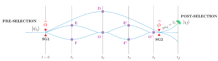
Figure 1: A 3 path interferometer for spin-1 particles with a provision for recombination of the 2 lower paths. Weak measurements take place at times $t_{k}$ (as indicated at the bottom) at the points shown on the figure. For appropriately chosen preselected and postselected states (see Text), null weak values are obtained at $O$ and $O^{\prime}$ but not at $E$, $F$, $E^{\prime}$ or $F^{\prime}$.

We can now compute the spatial projector weak values employing Eq. (10). Let $\Pi_{X}$ denote the spatial projector in the region $X,$ $\Pi_{X}=\left|\Gamma_{X}\right\rangle\left\langle\Gamma_{X}\right|$ that can be taken to be a Gaussian encompassing at most the spatial extent of the wavepacket, given by

$$\Gamma_{X}(\mathbf{r})=(\frac{2}{\pi\Delta^{2}})^{1/2}e^{-\left(\mathbf{r}-\mathbf{r}_{X}\right)^{2}/\Delta^{2}}.$$ (18)

The results are (see the time labels on Fig. 1)

$$t =t_{1}\text{ : }\Pi_{E}^{w}=1\qquad\Pi_{F}^{w}=-1$$ (19)

$$t =t_{2}\text{ : }\Pi_{D}^{w}=1\qquad\Pi_{O}^{w}=0$$ (20)

$$t =t_{3}\text{ : }\Pi_{E^{\prime}}^{w}=1\qquad\Pi_{F^{\prime}}^{w}=-1$$ (21)

$$t =t_{4}\text{ : }\Pi_{O^{\prime}}^{w}=0,$$ (22)

assuming the projector width $\Gamma_{X}(\mathbf{r})$ [Eq. (18)] overlaps with the spatial wavefunction (otherwise the ”ones” will be somewhat smaller than 1, though the null weak values remain $0$). The computation of these weak values is detailed in the Appendix.

Null weak values in Eqs. (19)-(22) are obtained at $O$ and $O^{\prime}$. $\Pi_{O^{\prime}}^{w}=0$ can be understood from the fact that the state vector going through $O^{\prime}$ is orthogonal to the postselection state. The transition amplitude $\left\langle\chi_{f}(t_{4})\right|\Pi_{O^{\prime}}\left|\psi(t_{4})\right\rangle$ vanishes implying that the final state $\left|\chi_{f}\right\rangle$ can therefore only be reached via the upper path with $k=+1$ (going through $D$). Now the state vector $\left|\psi(t_{4})\right\rangle$ going through $O^{\prime}$ results from the superposition of the wavepackets earlier localized at $E^{\prime}$ and $F^{\prime}$. Standard quantum mechanics tells us that the overall transition amplitude $\left\langle\chi_{f}(t_{3})\right|\left[\Pi_{E^{\prime}}+\Pi_{F^{\prime}}\right]\left|\psi(t_{3})\right\rangle$ vanishes but not the individual components $\left\langle\chi_{f}(t_{3})\right|\Pi_{E^{\prime}}\left|\psi(t_{3})\right\rangle$ and $\left\langle\chi_{f}(t_{3})\right|\Pi_{F^{\prime}}\left|\psi(t_{3})\right\rangle$ and hence the weak values (21) and (22) are non-null. The same reasoning applies to the weak values $\Pi_{E}^{w}$ and $\Pi_{F}^{w}$ that do not vanish – the pointers placed at points $E$ and $F$ will therefore move – while $\Pi_{O}^{w}=0$ and the quantum pointer coupled to the system there will not move. We interpret these results in Sec. IV.2 below, but it should be noted that if the weak values $\Pi_{X}^{w}$ are taken to account for the particle being not there or there according to whether the weak value is null or not, then we see that our weakly coupled pointers detect a particle inside the inner loop at $E^{\prime}$ and $F^{\prime}$ although no particle entered this inner loop (as it wasn’t detected by the pointer at $O$) and no particle went out (as no particle was detected by the pointer at $O^{\prime}$).

III.3.2 Nested Mach-Zehnder

The nested MZI example, introduced by Vaidman vaidman2013 , has been amply reproduced and discussed in several papers danan2013 ; zubairy2013 ; saldanha2014 ; vaidman-past ; bartkiewicz2015 ; ferenczi2015 ; jordan-dove ; sokolovskiMZI2016 ; griffiths2016 ; bula2016 , so we will only recall the main features. A photon enters a Mach-Zehnder interferometer (arms $C$ and $E$ in Fig. 2). A second MZI defining paths $A$ and $B$, is placed on arm $E$ (labeled $E^{\prime}$ behind the nested MZI). Postselection is defined by successful detection in port $D$. The weak values are

$$t =t_{1}\text{ : }\Pi_{C}^{w}=1\qquad\Pi_{E}^{w}=0$$ (23)

$$t =t_{2}\text{ : }\Pi_{A}^{w}=1\qquad\Pi_{B}^{w}=-1$$ (24)

$$t =t_{3}\text{ : }\Pi_{C^{\prime}}^{w}=1\qquad\Pi_{E^{\prime}}^{w}=0.$$ (25)

As in the previous example, the detector appears to be reached only by photons having taken arm $C$,on the ground that at $t=t_{3}$ previous to postselection, $\Pi_{E^{\prime}}^{w}=0$. However inside the nested MZI on the same arm, the weak values $\Pi_{A}^{w}$ and $\Pi_{B}^{w}$ are non-null (pointers detect the photon’s presence), although no photon can be detected coming in or coming out since the weak values at $E$ and $E^{\prime}$ vanish.

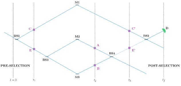
Figure 2: The nested Mach-Zehnder (MZ) interferometer setup. For an appropriately postselected state, null weak values are obtained at $E$ and $E^{\prime}$ (on the lower arm of the larger MZ) but not inside the nested MZ (the projector weak values on arms $A$ and $B$ are non-zero).

IV Discussion

IV.1 General remarks

The main issue arising from the examples depicted in Figs. 1 and 2 introduced in the preceding Section concerns the inference that can be made on the past of a particle’s motion based on the weak values. A solution to this issue will depend on a thorough understanding of the weak values (and more specifically on null weak values), and on being clear on the underlying interpretational assumptions that are sometimes implicitly made concerning the content of the standard formalism of quantum mechanics. The salient feature that calls for an explanation – irrespective of any stance regarding the status of weak values – is the fact that asymptotically weakly coupled pointers are triggered when placed inside the “loops” seen in Figs. 1 and 2, but they are left intact (ie, they do not detect anything) when placed ahead of or after the loop. We will not discuss here the explanations zubairy2013 ; saldanha2014 ; bartkiewicz2015 ; ferenczi2015 ; bula2016 given for the specific classical optics experiment reported in Ref. danan2013 , that do not touch the fundamental aspects we are focusing on in this work . From a fundamental standpoint, different approaches can be considered, ranging from denying weak values have any bearing on the particle properties (as properties hinge on a system being in an eigenstate of the relevant observable), to assuming null weak values are a manifestation of some novel underlying physics (like a wave coming from the future postselected state). We will mostly focus here on analyzing how null weak values can be interpreted.

IV.2 Interpretation of null weak values

IV.2.1 Null weak values for projection operators

As explained in Sec. III.2, a null weak value of a system observable $A$ is a statement about a vanishing transition amplitude that can be inferred from a quantum pointer coupled to $A$. If we are looking at the transition amplitude of $\Pi_{X}\equiv\left|X\right\rangle\left\langle X\right|$, then

$$\left\langle\chi(t_{w})\right|\Pi_{X}\left|\psi(t_{w})\right\rangle=\left\langle\chi(t_{f})\right|U(t_{f},t_{w})\Pi_{X}U(t_{w},t_{i})\left|\psi(t_{i})\right\rangle=0$$ (26)

is known from standard quantum mechanics to mean that the final state $\left|\chi(t_{f})\right\rangle$ cannot be reached from $\left|\psi(t_{i})\right\rangle$ by going through $X$. It is important to stress that this is a statement concerning the observable $\Pi_{X}$ (representing a physical property) and not the wavefunction. An analogy with classical optics (as proposed in Ref. saldanha2014 to describe the nested MZI of Sec. III.3.2) can at best be only partially useful, because although the classical and quantum waves take all the paths inside the interferometers, the classical electromagnetic wave is defined in physical space, whereas the quantum wavefunction is defined over an abstract configuration space and there is no consensus on its physical meaning . This is the reason measurements in quantum mechanics have a special status.

According to Eq. (26), the postselected state cannot be reached by the fraction of the system state coupled to the quantum pointer because that fraction evolved up to $t_{f}$, that is $U(t_{f},t_{w})\Pi_{X}U(t_{w},t_{i})\left|\psi(t_{i})\right\rangle$, is orthogonal to the postselected state. This property is not specific to weak measurements. Indeed Eq. (7) holds if the coupling is strong. Let us apply Eq. (7) with a strong coupling to the 3 path interferometer for a quantum pointer placed at $O,$ initially in state $\varphi_{O}(x,t_{i}).\$The postselected state is given by Eqs. (16)-(17) and $\Pi_{O}U(t_{2},t_{i})\left|\psi(t_{i})\right\rangle$ obtained from Eq. (34) is seen to be orthogonal to $\left\langle\chi(t_{w})\right|.$ Therefore Eq. (7) implies that

$$\varphi_{O}(x,t_{f})=\varphi_{O}(x,t_{i})$$ (27)

for each single run (for which postselection is obtained) – the quantum pointer has been left untouched by the strong coupling. This is unambiguously taken to mean that the particle did not go through $O$. Applying the same reasoning to a pointer strongly coupled to the particle at $D$ leads to $\varphi_{D}(x,t_{f})\varpropto\varphi_{D}(x+g,t_{i}):$ for each run the quantum pointer at $D$ acts as a detector that gets triggered, from which we conclude that the particle took path $D$ (indeed, $\Pi_{D}U(t_{2},t_{i})\left|\psi(t_{i})\right\rangle$ is not orthogonal to $\left\langle\chi(t_{2})\right|$). Now if the strongly coupled quantum pointer is placed instead at $E^{\prime}$ or $F^{\prime}$ (or for that matter at $E$ or $F$) there will be individual runs for which

$$\varphi_{E^{\prime}}(x,t_{f})\varpropto\varphi_{E^{\prime}}(x+g,t_{i})$$ (28)

indicating that the particle was along path $E^{\prime}$. Having Eqs. (27) and (28) is not seen as a contradiction because they can never be realized jointly for strong interactions (in a Bohrian like fashion, we would say that the conditions of the experiment are changed by inserting strongly coupled pointers at different positions, so as a whole we are not talking about the same physical situation).

In the asymptotically weak coupling limit however, all these conditions can be realized jointly, because the weak interactions do not break the system coherence. Arguably this cannot change the meaning of the transition amplitudes: if $\left\langle\chi(t_{2})\right|\Pi_{O}\left|\psi(t_{2})\right\rangle=0$ for a strong coupling implies that the system having evolved from the initial state $\left|\psi(t_{i})\right\rangle$ cannot be found at $O$ when detected in state $\left|\chi(t_{f})\right\rangle$, the same should hold for a weak coupling. The crucial difference between strong and weak couplings concerns the system’s state, not the transition amplitude: strong interactions drives the system to an eigenstate of the spatial projector, breaking the system coherence. The eigenstate-eigenvalue link can then hold. This is not the case for weak couplings, and this is precisely the reason the system coherence is not modified and that weak values $\Pi_{O}^{w}=0$ and $\Pi_{E^{\prime}}^{w}=1$ can be observed jointly. The bottom line is that the interpretation of a null weak value as reflecting the absence of a system property in the region in which the weak coupling took place hinges on one’s stance concerning quantum properties and the eigenvalue-eigenstate link (see Sec. IV.3.2).

In our view, the fact that weakly coupled quantum pointers can detect whether weak values are null or not are an indication that weak values can be regarded as physical but they convey a different property ascription than the one arising from the eigenstate-eigenvalue link. In the path integral approach, a functional represents the value of a system property along each path connecting the initial and final points, and the transition amplitude is obtained by summing the functional over all the available interfering paths (see Ch. 7 of feynman-hibbs ). The null weak value at $O\$in Fig. 1 can be understood in this way – the functional that takes opposite values on paths $E$ and $F$ so that $\Pi_{E}^{w}=-\Pi_{F}^{w}$ is summed at $O$ to yield a vanishing transition amplitude. From a quantum perspective, there is nothing paradoxical in measuring a null weak value at $O$ but not at $E$ and $E^{\prime}$: this appears as a consequence of taking the superposition principle seriously. If the system cannot go through $O$ and be detected in the postselected state, then we can say that “the particle was not there” provided “was” is employed in a liberal sense, because “the system is” is generally taken to mean “the system state is”, whereas here we are discerning a particular particle property correlated with a transition to a postselected state.

IV.2.2 Null weak values for general observables

While our focus up to now was on null weak values for projectors, most of what was written above holds also for null weak values of some general observable $A,$ Eq. (26) being replaced by

$$\left\langle\chi(t_{w})\right|A_{X}\left|\psi(t_{w})\right\rangle=\left\langle\chi(t_{f})\right|U(t_{f},t_{w})A_{X}U(t_{w},t_{i})\left|\psi(t_{i})\right\rangle=0,$$ (29)

the subscript $X$ indicating that $A$ is coupled to a quantum pointer in region $X$ (ideally, we could write $A_{X}\equiv\Pi_{X}A\Pi_{X}$ for a point like interaction at $X$). The main difference is that projectors have a null eigenvalue, rendering the connection between null weak values and eigenvalues of projectors more straightforward than for observables that do not possess a null eigenvalue. In particular the analogy made in Sec. IV.2.1 above between strong and weak couplings does not work, as a strong interaction couples the system eigenstates (with no null eigenvalue) to orthogonal pointer states. But the interpretation remains the same: the weak coupling changes the tiny fraction of the system state that couples to the quantum pointer into a state that will evolve to be orthogonal to the postselected state. In case of successful postselection, quantum correlations imply that the property represented by $A$ will not couple to a pointer located at $X$, and in this restricted sense, this property is “not there”. This conclusion is in line with Eq. (13) that tells us that the expectation value of $A$ at time $t_{w}$ can be obtained at time $t_{f}$ by measuring the observable $B$, but disregarding the eigenstates $\left|b_{f}\right\rangle$ for which the transition amplitude $\left\langle b_{f}\right|U(t_{f},t_{w})A\left|\psi(t_{w})\right\rangle$ vanishes.

To sum up, a null weak value should thus be understood as a statement concerning the absence of the property represented by the observable in the region in which the weak interaction took place, given the initial preparation and conditioned on final postselection. It is important to emphasize that a vanishing transition amplitude is to be associated with the absence of that specific property of the system that coupled to the weak pointer. This is sometimes forgotten when employing the “weak trace” criterion, as we now discuss.

IV.3 Inferring a particle’s past

IV.3.1 Weak trace criterion

The ”weak trace criterion” was defined in Ref. vaidman2013 as indicating the whereabouts of a detected particle (in a fixed postselected state) by looking at the weak trace left by the particle when locally coupled to a quantum pointer. The coupling should be minimally disturbing, ie sufficiently weak so that the coherence properties of the system are left unaffected. Standard quantum mechanics tells us, as reviewed in Sec. II, that the corresponding trace left on the quantum pointer’s state will precisely be the weak value of the system observable that coupled to the pointer. Of course, a quantum particle is not a classical point-like object, so we can expect to find simultaneous traces on different paths (like on the two arms of an usual Mach-Zehnder interferometer). But according to the weak trace criterion the particle was not in regions where the projector weak values vanished (and the relevant quantum pointers left intact). Now if this criterion is endorsed, the illustrations given above in which a particle leaves weak traces inside some inner loop, while no weak trace is left before or after the loop, calls for an explanation.

Vaidman suggests this “surprising” effect can be explained naturally by adopting an interpretative framework combining the two-state vector formalism (in which the weak values appear as the effective interaction due to the overlap of a preselected state evolving forward in time and a postselected state evolving backward in time) in the context of the many-worlds model vaidman2013 . Alonso and Jordan remarked jordan-dove that adding prisms on the arms of the nested interferometer in Fig. 2 did not change the weak values (23)-(25) but lead to detectable deflections at $E$ and $E^{\prime}\$. They wondered whether in a Wheeler-like fashion this effect could not be interpreted as the photon leaving retroactively a trace at $E$ depending on the presence of a prism inserted after the photon has left arm $E$ and entered the nested MZI.

Simpler explanations are available. First we remark that it is perfectly possible (and it is generally the case) to have at some point $X$ a vanishing spatial projector weak value in region $\Pi_{X}^{w}$ while the weak value of another observable $A$ (like a given spin component) measured at the same location is non-vanishing ($A^{w}\neq 0$). This is straightforward to implement in the 3 path interferometer by coupling at $O$ or $O^{\prime}$ an angular momentum component $J_{\gamma}$ (where $\mathbf{\hat{\gamma}}$ can be almost any arbitrary axis) to the quantum pointer; $\Pi_{O}^{w}=0$ and $\Pi_{O^{\prime}}^{w}=0$ will still hold, though the angular momentum weak values there $\left(J_{\gamma}\right)_{O}^{w}$ and $\left(J_{\gamma}\right)_{O^{\prime}}^{w}$ will be nonzero. In the nested MZI setup modified with prisms jordan-dove , it would arguably be simpler to write the relevant photon observable related to the selective deflection induced by the prism, and find that the corresponding weak values do not vanish at $E^{\prime}$ and $E^{\prime}$. Hence the weak trace criterion should be therefore be employed with reference to a specific system property. If we specify that we are inferring the particle’s past trajectory, since a trajectory is defined by the space-time points $\{t_{k},\mathbf{r}(t_{k})\}$, the relevant weak measurements are those related to the sole system position, and involve indeed the projection operators.

This brings us to the second point: a quantum particle is not a classical object (hence not even a particle in this sense). Inferring a particle’s past (and not only its past trajectory) should then involve the different properties that can be measured. Weak values of different observables will vanish at different locations. While detecting different properties in alternative locations would be startling for a classical particle, this is not so for an evolving quantum system envisaged as an extended undulatory entity whose local properties depend on interfering paths.

IV.3.2 Strong trace criterion

We term here “strong trace criterion” the scheme according to which a quantum particle’s past only makes sense when based on the eigenstate-eigenvalue link. This is remarkably the case of the Consistent Histories approach, whose starting point is to define a property from eigenvectors spanning the corresponding Hilbert space subspaces. Griffiths has recently given a Consistent Histories (CH) account of the nested MZI problem griffiths2016 . CH asserts that attempting to give an account of the particle’s presence inside the inner MZI is meaningless: the history family in which arms $A$ and $B$ of the inner MZI would be treated as mutually exclusive is inconsistent. This is to be expected whenever properties are grounded on assigning probabilities, and the CH framework precisely pinpoints what type of histories can describe an evolving quantum system and why two histories may be incompatible on this ground. While there is no place for weak measurements in the CH approach (given that weak measurements do not abide by the eigenstate-eigenvalue link), it would be instructive to see how CH explains the existence of weakly coupled pointers that measure quantities proportional to transition amplitudes. Unfortunately this is not done in Ref. griffiths2016 , where instead of weak measurements as introduced in Sec. II, strong interactions with a weak probability are discussed (the implications are examined in vaidman-com2016 ).

Employing a totally different framework also based ultimately on obtaining probabilities as specified by the eigenstate-eigenvalue link, Sokolovski sokolovskiMZI2016 does attempt to give a meaning to the weakly coupled pointers. In his view a path is real if a probability for taking a path can be obtained, but a path is virtual if only a transition amplitude can be attached to it. A strongly coupled meter creates real paths, while in the limit of small interactions a weakly coupled pointer picks up a “relative path amplitude” that has no bearing on the real interactions that have taken place. A vanishing transition amplitude at $X$ is then only relevant insofar as it indicates that a single standard strong pointer inserted at $X$ would not detect the particle there, but according to sokolovskiMZI2016 it is meaningless to make any assertion concerning the property of the system if interferences are not lifted by a strong coupling that will end up projecting the pointer to a state associated with a given system eigenstate.

The “strong trace criterion” fits well with the conventional view in which a property (represented by an observable) can only be ascribed to a quantum system when it is in an eigenstate of that observable. But from the start, the “strong trace criterion” discards any possibility to infer a property from protocols implementing non-destructive weak interactions. By restricting quantum properties ascription to changes of the state vector, the “strong trace criterion” has difficulties in giving a significance to the output of weakly coupled pointers that do not change the state of the system but give an indication of the value of an observable correlated with a detection in a postselected state. Indeed, such pointers, that can be experimentally observed, are then given a counterfactual significance (if a projective measurement would have been made instead then the result indicated by that particular weak pointer would have been obtained), a rather peculiar stance.

V Conclusion

In this work we have analyzed the properties and meaning of null weak values in the context of inferring the past of a quantum particle from interactions of the system with weakly coupled pointers. A null weak value of an observable $A$ obtained at some location $X$ means that the system property represented by $A$ cannot be found at $X$ and detected in the postselected state. The past of a quantum particle can be inferred by taking into account all of its observables, not only spatial projectors. The fact that discontinous traces of a given property can be experimentally observed from weakly coupled pointers seems to be an indication that the wavefunction superposition is related to a physical phenomenon, rather than being a mere computational artifact.

Appendix A Weak values in the 3-path interferometer

We detail here the computation of the weak values for the 3 path interferometer described in Sec. III.3.1. As an example, let us give the calculation for the weak values at $t=t_{2}.$ We have by the very definition Eq. (10)

$$\Pi_{D}^{w}=\frac{\left\langle\chi_{f}(t_{f})\right|U(t_{f},t_{2})\Pi_{D}U(t_{2},t_{i})\left|\psi_{i}\right\rangle}{\left\langle\chi_{f}(t_{f})\right|U(t_{f},t_{2})U(t_{2},t_{i})\left|\psi_{i}\right\rangle}.$$ (30)

Then keeping in mind that $\Pi_{D}\left|\xi_{k}(t_{2})\right\rangle=0$ for $k=0,-1$ Eq. (15) leads to

$$\Pi_{D}^{w}=\frac{\left\langle\xi_{f}(t_{f})\right|U(t_{f},t_{2})\Pi_{D}\left|\xi_{k=+1}(t_{2})\right\rangle d_{1}(\alpha)\left\langle m_{f}\right|\left.m_{\alpha}=1\right\rangle}{\sum_{k=-1}^{1}d_{k}(\alpha)\left\langle m_{f}\right|\left.m_{\alpha}=k\right\rangle}$$ (31)

that simplifies given our choice of $\left|m_{f}\right\rangle,$ encapsulated by the condition (17) to

$$\Pi_{D}^{w}=\left\langle\xi(t_{f})\right|U(t_{f},t_{2})\Pi_{D}\left|\xi_{A}(t_{2})\right\rangle\approx 1.$$ (32)

For the weak value in the region $O$ we have

$$\Pi_{O}^{w}=\frac{\left\langle\chi_{f}(t_{f})\right|U(t_{f},t_{2})\Pi_{O}U(t_{2},t_{i})\left|\psi_{i}\right\rangle}{\left\langle\chi_{f}(t_{f})\right|U(t_{f},t_{2})U(t_{2},t_{i})\left|\psi_{i}\right\rangle}.$$ (33)

Following Eq. (15), $U(t_{2},t_{i})\left|\psi_{i}\right\rangle$ is of the form

$$U(t_{2},t_{i})\left|\psi_{i}\right\rangle=d_{1}(\alpha)\left|m_{\alpha}=+1\right\rangle\left|\xi_{D}(t_{2})\right\rangle+\sum_{k=-1,0}d_{k}(\alpha)\left|m_{\alpha}=k\right\rangle\left|\xi_{O}(t_{2})\right\rangle$$ (34)

and $\Pi_{O}\left|\xi_{D}(t_{2})\right\rangle$ vanishes (since there is no spatial overlap between $\left|\Gamma_{O}\right\rangle$ and $\left|\xi_{D}(t_{2})\right\rangle$). The weak value becomes

$$\Pi_{O}^{w}=\frac{\left\langle\xi(t_{f})\right|U(t_{f},t_{2})\Pi_{O}\left|\xi_{O}(t_{2})\right\rangle}{\left\langle\chi_{f}(t_{f})\right|U(t_{f},t_{2})U(t_{2},t_{i})\left|\psi_{i}\right\rangle}\left[\sum_{k=-1,0}d_{k}(\alpha)\left\langle m_{f}\right|\left.m_{\alpha}=k\right\rangle\right]=0;$$ (35)

indeed, the square bracket in this equation vanishes, since this is precisely the condition (17) imposed for the postselection state.

The other weak values given in Eqs. (19)-(22) are computed in the same way.

References

- (1) N. Bohr. Albert Einstein: Philosopher-Scientist, chapter 7. MJF Books, New York, 1949.
- (2) J. A. Wheeler. chapter 1.13. Princeton University Press, Princeton (New Jersey), USA, 1983.
- (3) L. Vaidman. Phys. Rev. A, 87:052104, 2013.
- (4) A. Matzkin. Phys. Rev. Lett., 109:150407, 2012.
- (5) Y. Aharonov, D. Z. Albert, and L. Vaidman. Phys. Rev. Lett., 60:1351, 1988.
- (6) J. Dressel, M. Malik, F. M. Miatto, A. N. Jordan, and R. W. Boyd. Rev. Mod. Phys., 86:304, 2014.
- (7) A. J. Leggett. Phys. Rev. Lett., 62:2325, 1989.
- (8) A. Peres. Phys. Rev. Lett., 62:2326, 1989.
- (9) D. Sokolovski. Phys. Lett. A, 380:1593, 2016.
- (10) B. E. Y. Svensson. Phys. Script., 2014:014025, 2014.
- (11) A. Matzkin and A. K. Pan. J. Phys. A: Math. Theor., 46:315307, 2013.
- (12) Z.-H. Li, M. Al-Amri, and M. S. Zubairy. Phys. Rev. A, 88:046102, 2013.
- (13) L. Vaidman. Phys. Rev. A, 88:046103, 2013.
- (14) P. L. Saldanha. Phys. Rev. A, 89:033825, 2014.
- (15) K. Bartkiewicz, A. Černoch, D. Javrek, K. Lemr, J. Soubusta, and J. Svozilík. Phys. Rev. A, 91:012103, 2015. See also the ensuing Comment and Reply: L. Vaidman, Phys. Rev. A 93, 036103, 2016; K. Bartkiewicz, A. Černoch, D. Javrek, K. Lemr, J. Soubusta, and J. Svozilík, Phys. Rev. A 93, 036104, 2016.
- (16) V. Potoček and G. Ferenczi. Phys. Rev. A, 92:023829, 2015.
- (17) M. A. Alonso and A. N. Jordan. Quantum Stud.: Math. Found., 2:255, 2015.
- (18) D. Sokolovski. arXiv:1607.03732, 2016.
- (19) R. B. Griffiths. Phys. Rev. A, 94:032115, 2016.
- (20) M. Bula, K. Bartkiewicz, A. Černoch, D. Javrek, K. Lemr, V. Michálek, and J. Soubusta. Phys. Rev. A, 94:052106, 2016.
- (21) L. Vaidman. arXiv:1610.07734, 2016.
- (22) A. Danan, D. Farfurnik, S. Bar-Ad, and L. Vaidman. Phys. Rev. Lett., 111:240402, 2013.
- (23) L. Vaidman. Phys. Rev. A, 89:024102, 2014.
- (24) A. K. Pan and A. Matzkin. Phys. Rev. A, 85:022122, 2012.
- (25) B. G. Englert, J. Schwinger, and M. O. Scully. Found. Phys., 18:1045, 1988.
- (26) R. Mathevet, K. Brodsky, J. Baudon, R. Brouri, M. Boustimi, B. V. de Lesegno, and J. Robert. Phys. Rev. A, 58:4039, 1998.
- (27) A. Matzkin. Eur. J . Phys., 23:285, 2002.
- (28) R. P. Feynman and A. R. Hibbs. Quantum Mechanics and Path Integrals. McGraw-Hill, New York, U.S.A., 1965.