Second-Harmonic Imaging in Random Media

Abstract.

We consider the problem of optical imaging of small nonlinear scatterers in random media. We propose an extension of coherent interferometric imaging (CINT) that applies to scatterers that emit second-harmonic light. We compare this method to a nonlinear version of migration imaging and find that the images obtained by CINT are more robust to statistical fluctuations. This finding is supported by a resolution analysis that is carried out in the setting of geometrical optics in random media. It is also consistent with numerical simulations for which the assumptions of the geometrical optics model do not hold.

1. Introduction

1.1. Background

There has been considerable recent interest in the development of methods for optical imaging of biological systems in the mesoscopic scattering regime [1]. There are multiple potential applications incuding imaging of engineered tissues and semitransparent organisms, such as Drosophila and zebra fish, among others [2]. Here the term mesoscopic refers to systems whose size is of the order of the transport mean free path of light [3, 4]. In this setting, light exhibits sufficiently strong scattering so that direct imaging is not possible. Moreover, imaging modalities that rely on diffuse propagation of light are not effective. Thus, optical imaging techniques that bridge the gap between microscopic and macroscopic scales are of increasing importance.

Mesoscopic imaging may be carried out using either coherent or incoherent approaches. Incoherent methods, which make use of intensity measurements of transmitted light, include confocal microscopy, optical projection tomography and single-scattering optical tomography [1, 11, 13, 15, 16, 17, 18, 19, 20, 21]. Coherent methods, which additionally rely on measurements of the optical phase, include optical coherence microscopy and interferometric synthetic aperture microscopy [12, 14].

An important refinement of optical imaging is to introduce a fluorescent molecular probe that binds to a target of interest. In this manner, spectral isolation and increased signal-to-noise of the detected light can be achieved [2]. Spectral isolation may also be realized by utilizing a contrast agent that exhibits a nonlinear optical response. This approach has the advantage that it is not affected by fluorescent photobleaching. Experiments in which second-harmonic generation (SHG) has been utilized for mesoscopic imaging have recently been reported [22, 23]. The theory of SHG is reviewed in [24]. Briefly, second-harmonic light is generated by a nonlinear process in which the polarization of a material medium depends both linearly and quadratically on the electric field.

In this paper we introduce a new form of coherent mesoscopic imaging, in which interferometric measurements are used to localize small scatterers that emit second-harmonic light. The scatterers are embedded in an unknown background medium, that is taken to be random. The method that is proposed is an extension of coherent interferometry (CINT) to media that exhibit a nonlinear response. The key idea of CINT is to form images by backpropagating correlations of the measured field [27, 28]. We compare nonlinear CINT to a nonlinear version of migration imaging, in which the fields alone are backpropagated [10]. We find that the images obtained by CINT are more robust to statistical fluctuations in the background medium in comparison to images obtained by migration. This conclusion is supported by an analysis of image resolution carried out within the framework of a model for geometrical optics in random media. It is also consistent with numerical simulations of wave propagation in media for the which the assumptions of the geometrical optics model do not hold. We note that migration imaging for nonlinear media was also studied in [25]. However, in that work, only migration imaging was investigated in the setting of a two-dimensional model for SHG with transverse-magnetic polarization for the incident field and transverse-electric polarization for the second harmonic.

1.2. Physical principles

We are interested in imaging small nonlinear scatterers at positions $\bm{y}_{j}$, for $j=1,\ldots,N_{y}$, in a medium occupying a bounded domain $V\subset\mathbb{R}^{m}$, with boundary $\partial V$, for $m\geq 2$, as illustrated in Figure 1. We restrict our attention to the case of second harmonic generation (SHG), but more general, quadratic or cubic nonlinearities could be treated similarly. For convenience, we let $V$ be a cube (or square in two dimensions) of side $2L$. The medium in $V$ is illuminated by monochromatic plane waves at frequency $\omega$, in the directions of the unit vectors ${\bm{\theta}}_{j}$, for $j=1,\ldots,N_{\theta}$. These vectors belong to a cone $C$ with axis along the unit vector $\bm{\vartheta}$ normal to $\partial V$, and small opening angle $\alpha$. The resulting waves are measured by an array of detectors located at points $\bm{x}_{s}$ in the array aperture ${A}$, for $s=1,\ldots,N_{\bm{x}}$. The array lies on one side of the boundary $\partial V$, and $A$ is a square of side $a\ll L$, or a segment of length $a\ll L$ in two dimensions. In the analysis, not the numerics, we suppose that the scatterers are confined to a cubic (square) region $R$ with the same center as $V$, of side $r\ll L$. We also let the centers of $A$ and $V$ be lined up along the unit normal vector ${\bm{n}}$, which is orthogonal to $\bm{\vartheta}$ and the array aperture.

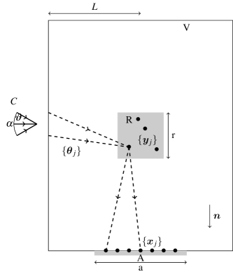
Figure 1. Setup of the imaging problem. $A$ denotes the array, $C$ the cone of incident directions, $R$ the search region and $V$ the imaging domain.

The imaging problem is to estimate the locations of the $N_{\bm{y}}$ nonlinear scatterers from the measurements of the wave fields at the array, at frequency $\omega$ and the second harmonic $2\omega$. When the medium in $V$ is known and is non-scattering, we can image with coherent methods known as matched filtering in the signal processing [39] and radar literature [35], migration in seismic imaging [9], and backprojection in computed tomography [34]. These methods form an image by superposing the array measurements backpropagated in the known medium to imaging points $\bm{y}^{R}$ in $R$. The backpropagation is done analytically when the Green’s function is known, or numerically, and its purpose is to compensate for the phases of the measurements at points $\bm{y}^{R}$ near the scatterer location, so that they add constructively, and the imaging function displays a peak. We refer henceforth to such imaging as migration.

In this paper we consider the problem of imaging in heterogeneous media, containing numerous small inhomogeneities. A single inhomogeneity by itself is assumed to be much weaker than the scatterer that we wish to image. However, the waves interact with many inhomogeneities over the $O(L)$ distances of propagation, and this results in strong cumulative scattering effects that must be taken into account in imaging. This problem is challenging because, in applications, it is impossible to know the numerous inhomogeneities, and we cannot hope to determine them from the data. Thus, imaging is carried in an uncertain environment. We incorporate this uncertainty in the data model by studying imaging in random media. The goal is to understand whether it is possible to obtain robust estimates of the nonlinear scatterer locations from the measurements registered by the array in a fixed realization of the random medium. Such robustness is known as statistical stability, and it means that the images vary little from one realization of the random medium to another.

Our results consist of analysis and numerical simulations of imaging of nonlinear scatterers in a random medium. We consider two regimes where cumulative scattering by the inhomogeneities causes large distortion of the wave field measured at the array. In physical terms, this means that $L$ is larger than the scattering length (also known as scattering mean free path) ${\it\ell^{s}}$, which is the characteristic length scale on which the waves randomize [3]. The analysis uses a geometrical optics model [38], where the typical size $\ell$ of the inhomogeneities is large with respect to the wavelength $\lambda$, and $L\gg{\it\ell^{s}}\gg\ell$, so that the net scattering effects in the medium amount to large random wavefront distortions. In the numerics we consider a regime with $\ell\sim\lambda$, where the waves interact more efficiently with the inhomogeneities. Because we are interested in coherent imaging, we take $L$ of the order of the transport mean free path, which is the characteristic distance at which the waves forget their initial direction due to scattering [3]. As explained above, this corresponds to the mesoscopic regime. At larger distances, the waves are in a radiative transfer regime, and only incoherent imaging methods are effective [1].

We find in both the analysis and numerical simulations that the statistical fluctuations of the array measurements due to scattering in the random medium are very different than those of additive noise. They cannot be mitigated simply by summation of the measured fields, as in migration. Ideally, the fluctuations could be treated by backpropagation of the measurements in the medium, as in time reversal [32]. However, this cannot be done because the medium is unknown. We can only backpropagate in a hypothetical reference medium with known wave velocity, which is constant in this paper, and thus obtain migration images. We show that these images are statistically unstable, meaning that they change significantly and unpredictably from one realization of the random medium to another.

The coherent interferometric (CINT) method [28, 29] is designed to ameliorate the effects of random wave distortions, by imaging with cross-correlations of the measurements instead of the measurements themselves. The CINT imaging function is given by the superposition of cross-correlations backpropagated in the reference medium. Its mathematical expression resembles that of the time reversal function analyzed in [36, 37], and its statistical stability and resolution are studied in [29, 27]. Unlike in time reversal, where super-resolution of focusing occurs, the stability of CINT comes at the expense of resolution, which is determined by two characteristic scales in the random medium: the decoherence frequency and length. These scales describe the frequency offsets and detector separations over which the waves become statistically uncorrelated, and must be taken into account in the calculation of the cross-correlations [28]. Moreover, they determine the conditions under which CINT is statistically stable. This can be formally understood as a consequence of the law of large numbers, due to the summation in the imaging function of many statistically uncorrelated terms, when the array aperture is much larger than the decoherence length, and the probing signals have bandwidth that is larger than the decoherence frequency [29].

In this paper we study CINT imaging with time harmonic waves, so summation over frequencies is not carried out. Such a summation is essential for the statistical stability of CINT, and of time reversal for that matter [26], when scattering in the medium causes significant delay spreading. Here we consider weaker scattering regimes, like random geometrical optics, where imaging can be performed at a single frequency [27].

The remainder of this paper is organized as follows. In Section 2, we present the formulation of the problem and introduce the necessary migration and CINT imaging formalism. In Section 3, we analyze the migration and CINT point spread functions in the setting of the random geometrical optics model. Section 4 presents our numerical results for two-dimensional model systems. We end with a summary in Section 5. The appendices present some technical details and derivations of results presented in the paper.

2. Formulation of the problem

In this section we describe the model of the imaging experiment and define the migration and CINT imaging functions that are analyzed theoretically and numerically in the following sections.

2.1. Random model of the array data

We consider for simplicity scalar waves, that obey the Helmholtz equation with a random wave speed $c(\bm{x})$ of the form

$$c(\bm{x})=c_{0}\left[1+4\pi\eta(\bm{x})\right]^{-1/2},$$ (2.1)

where $c_{0}$ is constant and $\eta(\bm{x})$ is the linear susceptibility of the medium. Here $\eta(\bm{x})$ is taken to be a mean zero, stationary random process that is bounded almost surely, so that the right hand side in (2.1) remains positive. We also assume that $\eta(\bm{x})$ is mixing (lacks long range correlations) [33], with integrable autocorrelation function. The small scatterers embedded in the random medium with wave speed (2.1) are modeled by the linear susceptibility $\eta_{1}(\bm{x})$ and quadratic susceptibility $\eta_{2}(\bm{x})$. These are functions with small amplitude and support concentrated in the vicinity of the points $\bm{y}_{j}$, for $j=1,\ldots N_{\bm{y}}$.

Under conditions of weak nonlinearity, the linear and second harmonic wave fields obey [24]

$$\Delta u_{1}(\bm{x};{\bm{\theta}})+k^{2}[1+4\pi\eta(\bm{x})]u_{1}(\bm{x};{\bm{\theta}}) =-4\pi k^{2}[\eta_{1}(\bm{x})u_{1}(\bm{x};{\bm{\theta}})+2\eta_{2}(\bm{x})u_{2}(\bm{x};{\bm{\theta}})u_{1}^{*}(\bm{x};{\bm{\theta}})]\ ,$$ (2.2)

$$\Delta u_{2}(\bm{x};{\bm{\theta}})+(2k)^{2}[1+4\pi\eta(\bm{x})]u_{2}(\bm{x};{\bm{\theta}}) =-4\pi(2k)^{2}[\eta_{1}(\bm{x})u_{2}(\bm{x};{\bm{\theta}})+\eta_{2}(\bm{x})u_{1}^{2}(\bm{x};{\bm{\theta}})],$$ (2.3)

for $\bm{x}\in V$. Here $u_{1}(\bm{x};{\bm{\theta}})$ is the wave at frequency $\omega$ and $u_{2}(\bm{x};{\bm{\theta}})$ is the wave at the second harmonic $2\omega$. The medium is illuminated by $N_{\theta}$ plane waves at frequency $\omega$

$$u_{1,0}^{(i)}(\bm{x};{\bm{\theta}}_{q})=e^{ik{\bm{\theta}}_{q}\cdot\bm{x}},$$ (2.4)

where $k=\omega/c_{0}$ is the wavenumber and ${\bm{\theta}}_{q}$ are unit wave vectors. The scattered waves, given by $u_{1}(\bm{x};{\bm{\theta}}_{q})-u_{1,0}^{(i)}(\bm{x};{\bm{\theta}}_{q})$ and $u_{2}(\bm{x};{\bm{\theta}}_{q})$, satisfy outgoing boundary conditions on $\partial V$.

The imaging is to be carried using measurements of the wave fields at the $N_{\bm{x}}$ detectors in the array, gathered in the set

$$\mathcal{U}=\left\{u_{1}(\bm{x}_{s};{\bm{\theta}}_{q}),~{}u_{2}(\bm{x}_{s};{\bm{\theta}}_{q}),~{}~{}~{}s=1,\ldots,N_{\bm{x}},~{}~{}q=1,\ldots,N_{\theta}\right\}.$$ (2.5)

Note that $u_{1}(\bm{x};{\bm{\theta}}_{q})$ and $u_{2}(\bm{x};{\bm{\theta}}_{q})$ are random fields, and the actual array measurements are for a single realization of the medium. These are the data used to form images, as explained in the next sections. We only use the set $\mathcal{U}$ for the statistical analysis of the imaging functions.

2.2. Migration imaging

In migration imaging one assumes that the background medium is known and non-scattering, and that the waves are reflected once at the unknown scatterers. In our setting this corresponds to assuming that $\eta\equiv 0$ in (2.1), and using the Born approximation with respect to $\eta_{1}(\bm{x})$ and $\eta_{2}(\bm{x})$ in equations (2.3). We obtain the linearized forward mappings from the unknown susceptibilities $\eta_{1}(\bm{x})$ and $\eta_{2}(\bm{x})$ to the scattered fields at the array

$$F_{j}[\eta_{j}](\bm{x}_{s},{\bm{\theta}}_{q})=(jk)^{2}\int_{V}d\bm{y}\,\eta_{j}(\bm{y})G_{0}(\bm{x}_{s},\bm{y};j\omega)e^{ijk{\bm{\theta}}_{q}\cdot\bm{y}},\qquad j=1,2,$$ (2.6)

where $G_{0}$ is the outgoing Green’s function, given by

$$G_{0}(\bm{x},\bm{y};\omega)=\frac{e^{ik|\bm{x}-\bm{y}|}}{|\bm{x}-\bm{y}|}$$ (2.7)

in three dimensions, and by

$$G_{0}(\bm{x},\bm{y};\omega)=i\pi H_{0}^{(1)}(k|\bm{x}-\bm{y}|)$$ (2.8)

in two dimensions, where $H_{0}^{(1)}$ is the Hankel function of the first kind. The mappings in (2.6) are evaluated at the detector locations indexed by $s=1,\ldots,N_{\bm{x}}$, and at the incident plane wave vectors indexed by $q=1,\ldots,N_{\theta}$. The index $j=1,2$ corresponds to the frequencies by $j\omega$.

Let us denote by $d_{1}$ and $d_{2}$ the data for inversion, given by

$$d_{1}(\bm{x}_{s},{\bm{\theta}}_{q}) \approx u_{{}_{1}}^{(real)}(\bm{x}_{s};{\bm{\theta}}_{q})-u_{1,0}^{(i)}(\bm{x}_{s};{\bm{\theta}}_{q}),$$ (2.9)

$$d_{{}_{2}}(\bm{x}_{s},{\bm{\theta}}_{q}) \approx u_{{}_{2}}^{(real)}(\bm{x}_{s};{\bm{\theta}}_{q}),\quad s=1,\ldots,N_{\bm{x}},~{}~{}q=1,\ldots,N_{\theta},$$ (2.10)

where $u_{j}^{(real)}$, for $j=1,2$, denote the measurements in the real medium, one realization of the random model. The approximation sign accounts for noise that is unavoidable in experiments. When this noise is additive, mean zero, identically distributed, with finite variance, the Gauss-Markov theorem gives that the best unbiased linear estimator of the unknown susceptibilities is the solution of the least squares problem [40]

$$\eta_{j}^{{}^{LS}}=\underset{\eta_{j}}{\mbox{arg min}}\,\|d_{j}-F_{j}[\eta_{j}]\|_{2}^{2}.$$ (2.11)

The minimizers $\eta_{j}^{{}^{LS}}$ satisfy the normal equations

$$F_{j}^{H}F_{j}[\eta_{j}^{{}^{LS}}](\bm{y}^{R})=F_{j}^{H}[d_{j}](\bm{y}^{R})=(jk)^{2}\sum_{s=1}^{N_{\bm{x}}}\sum_{q=1}^{N_{\theta}}G_{0}^{\star}(\bm{y}^{R},\bm{x}_{s};j\omega)e^{-ijk{\bm{\theta}}_{q}\cdot\bm{y}^{R}}d_{j}(\bm{x}_{s},{\bm{\theta}}_{q}),$$ (2.12)

where the superscript $H$ denotes the adjoint with respect to the Euclidian inner product. The integral (normal) operators $F_{j}^{H}F_{j}$ map $\eta_{j}^{{}^{LS}}$ to

$$F_{j}^{H}F_{j}[\eta_{j}^{{}^{LS}}](\bm{y}^{R})=\int_{V}d\bm{y}\,\eta_{j}^{{}^{LS}}(\bm{y})\mathcal{K}_{j}(\bm{y}^{R},\bm{y}),$$ (2.13)

and their integral kernels

$$\mathcal{K}_{j}(\bm{y}^{R},\bm{y})=(jk)^{4}\sum_{s=1}^{N_{\bm{x}}}\sum_{q=1}^{N_{\theta}}G_{0}(\bm{x}_{s},\bm{y};j\omega)G^{\star}_{0}(\bm{y}^{R},\bm{x}_{s};j\omega)e^{ijk{\bm{\theta}}_{q}\cdot(\bm{y}-\bm{y}^{R})}$$ (2.14)

are equal, up to constant factors, to the time reversal point spread functions at frequencies $j\omega$, for $j=1,2$. In our setting, the kernels (2.14) peak along the diagonal $\bm{y}^{R}=\bm{y}$, so we can approximate the left hand side in (2.13) by $\eta_{j}^{{}^{LS}}(\bm{y}^{R})$ multiplied by a constant.

In imaging, we are interested in the support of the sussceptibilities, so we can neglect the constants and obtain from (2.14) the migration imaging functions

$$\mathcal{I}^{{M}}_{{}_{j}}(\bm{y}^{R})=\sum_{s=1}^{N_{\bm{x}}}\sum_{q=1}^{N_{\theta}}G_{0}^{\star}(\bm{y}^{R},\bm{x}_{s};j\omega)e^{-ijk{\bm{\theta}}_{q}\cdot\bm{y}^{R}}d_{j}(\bm{x}_{s},{\bm{\theta}}_{q}),\quad j=1,2.$$ (2.15)

Since $k|\bm{y}^{R}-\bm{x}_{s}|\gg 1$ and the array aperture size $a$ is much smaller than $|\bm{x}_{s}-\bm{y}^{R}|=O(L)$, for $\bm{y}^{R}$ in the search region $R$ (recall Figure 1), we can approximate the Green’s function in (2.15) by

$$G_{0}(\bm{y}^{R},\bm{x}_{s};j\omega)\approx C_{j}e^{ijk|\bm{y}^{R}-\bm{x}_{s}|},$$ (2.16)

for constant $C_{j}$, with $j=1,2$. This result holds in both two and three dimensions, as follows from the asymptotics of the Hankel function in (2.8). Thus, the right hand side of (2.15) is the superposition of the measurements, with phases given relative to the imaging point $\bm{y}^{R}$. The superposition is needed for focusing the image and averaging over the noise. When $\bm{y}^{R}$ is close to a scatterer location, and the medium is either homogeneous or has negligible effect on the waves, so that their propagation is approximated by $G_{0}$, the phases in $d_{j}$ are cancelled approximately. Then, the terms in (2.15) add constructively and the imaging function displays a peak. In this paper we are interested in imaging in stronger scattering media, where $G_{0}$ is not a good model for wave propagation, and the migration imaging function (2.15) either does not focus, or gives spurious peaks at locations that may not be close to the scatterers.

2.3. Coherent interferometric imaging

Let $\bm{y}^{R}$ be an imaging point and define

$$b_{j}(\bm{x}_{s},{\bm{\theta}}_{q},\bm{y}^{R})=d_{j}(\bm{x}_{s},{\bm{\theta}}_{q})G_{0}^{\star}(\bm{y}^{R},\bm{x}_{s};j\omega)e^{-ijk{\bm{\theta}}_{q}\cdot\bm{y}^{R}},$$ (2.17)

for detector index $s=1,\ldots,N_{\bm{x}}$, plane wave index $q=1,\ldots,N_{\theta}$, and frequency index $j=1,2.$ The CINT imaging function is formed by superposition of local cross-correlations of $b_{j}$. By local we mean that we cross-correlate only at nearby detectors and for nearby incident directions

$$|\bm{x}_{s}-\bm{x}_{s^{\prime}}|\leq X,\quad|{\bm{\theta}}_{q}-{\bm{\theta}}_{q^{\prime}}|\leq\Theta,$$ (2.18)

where $\Theta$ and $X$ are scales that account for the decorrelation of the waves due to scattering in the random medium [28]. Intuitively, in the language of geometrical optics, waves traveling along different paths are decorrelated because they interact with different parts of the random medium, assumed to lack long range correlations of the fluctuations of the wave speed. Note that in practice the scales of decorrelation of the waves are usually unknown, so they must be estimated from the data, either using statistical data analysis or by optimization, which seeks to improve the focusing of CINT images, as explained in [28]. We denote henceforth the true decorrelation parameters in the medium by $X_{d,j}$ and $\Theta_{d}$, to distinguish them from those used in the calculation of the cross-correlations, and assume that

$${X}/{X_{d,j}}=O(1),\quad{\Theta}/{\Theta_{d}}=O(1).$$ (2.19)

We also refer to $X_{d,j}$ as decoherence lengths and $\Theta_{d}$ as decoherence angle. Note that the decoherence length is proportional to the wavelength, so it depends on $j$. We suppress, for simplicity of notation, the dependence of the thresholding parameter $X$ on $j$.

Let us introduce the center and offset sensor locations

$$\overline{\bm{x}}_{ss^{\prime}}=({\bm{x}_{s}+\bm{x}_{s^{\prime}}})/{2},\quad\widetilde{\bm{x}}_{ss^{\prime}}=\bm{x}_{s}-\bm{x}_{s^{\prime}},\quad s,s^{\prime}=1,\ldots,N_{\bm{x}},$$ (2.20)

and direction vectors

$$\overline{\bm{\theta}}_{qq^{\prime}}=({{\bm{\theta}}_{q}+{\bm{\theta}}_{q}^{\prime}})/{2},\quad\widetilde{\bm{\theta}}_{qq^{\prime}}={\bm{\theta}}_{q}-{\bm{\theta}}_{q^{\prime}},\quad q,q^{\prime}=1,\ldots,N_{\theta}.$$ (2.21)

We count the center variables by $\overline{s}=1,\ldots,\overline{N}_{{}_{\bm{x}}}$ and $\overline{q}=1,\ldots,\overline{N}_{{}_{\theta}}$, and the offsets by $\widetilde{s}=1,\ldots,\widetilde{N}_{{}_{\bm{x}}}$ and $\widetilde{q}=1,\ldots,\widetilde{N}_{{}_{\theta}}$. The local cross-correlations are

$$\mathcal{C}_{j}(\overline{\bm{x}}_{\overline{s}},\overline{\bm{\theta}}_{\overline{q}},\bm{y}^{R})=\sum_{\widetilde{s}=1}^{\widetilde{N}_{{}_{\bm{x}}}}\sum_{\widetilde{q}=1}^{\widetilde{N}_{\theta}}\Phi\Big{(}\frac{\widetilde{\bm{x}}_{\widetilde{s}}}{X}\Big{)}\Phi\Big{(}\frac{\widetilde{\bm{\theta}}_{\widetilde{q}}}{\Theta}\Big{)}b_{j}\Big{(}\overline{\bm{x}}_{\overline{s}}+\frac{\widetilde{\bm{x}}_{\widetilde{s}}}{2},\overline{\bm{\theta}}_{\overline{q}}+\frac{\widetilde{\bm{\theta}}_{\widetilde{q}}}{2},\bm{y}^{R}\Big{)}b_{j}^{\star}\Big{(}\overline{\bm{x}}_{\overline{r}}-\frac{\widetilde{\bm{x}}_{\widetilde{s}}}{2},\overline{\bm{\theta}}_{\overline{q}}-\frac{\widetilde{\bm{\theta}}_{\widetilde{q}}}{2},\bm{y}^{R}\Big{)},$$ (2.22)

where $\Phi$ is a smooth window of support of order one, used to limit the detector and director offsets by $X$ and $\Theta$. The CINT imaging function is formed by the superposition of (2.22),

$$\mathcal{I}^{{CINT}}_{{}_{j}}(\bm{y}^{R})=\sum_{\overline{s}=1}^{\overline{N}_{s}}\sum_{\overline{q}=1}^{\overline{N}_{\theta}}\mathcal{C}_{j}(\overline{\bm{x}}_{\overline{s}},\overline{\bm{\theta}}_{\overline{q}},\bm{y}^{R}).$$ (2.23)

Were it not for the windows $\Phi$ in (2.22), this expression would equal the square of the migration imaging function (2.15). The windows play a smoothing role in (2.23), by convolution. This blurs the images, but is essential for stabilizing them statistically [29].

Remark 1.

The phase compensation in equation  (2.17) assumes the complete removal of the direct waves that have not interacted with the scatterers that we wish to image. In homogeneous media this is achieved by the subtraction of the incident wave $u_{1,0}^{(i)}$ from the measurements. However, this wave is affected by scattering in random media, so the subtraction in (2.9) does not achieve its purpose. The unwanted direct wave may be removed in our geometrical setting if the array of detectors can differentiate among arrival directions, and the scattering medium is not strong enough to mix the directions of the waves, as is the case in the geometrical optics regime considered in our analysis. Such differentiation may be achieved for example by an approximate plane wave decomposition of the measurements, using a discrete Fourier transform with respect to the coordinates of the detectors in the array. We do not perform such a differentiation here and work instead with (2.9), to illustrate the effect of the unwanted direct arrivals on the imaging of $\eta_{1}$. This problem does not extend to the second harmonic wave (2.10), which is emitted at the nonlinear scatterers.

3. Analysis of the migration and CINT point spread functions

In this section we analyze migration and CINT imaging of a single scatterer at location $\bm{y}$ in $V$. This means that we analyze the point spread functions of (2.15) and (2.23). We consider a geometrical optics wave propagation regime, with large random distortions of the wavefront. The analysis is in most respects the same in two and three dimensions, so we focus our attention on the three dimensional case.

To begin, we write the susceptibility of the medium as

$$4\pi\eta(\bm{x})=\sigma\mu\left(\frac{\bm{x}}{\ell}\right),$$ (3.1)

where $\mu$ is a random, stationary process with mean zero and Gaussian autocorrelation

$$\mathbb{E}[\mu(\bm{h})\mu(\bm{0})]=e^{-\frac{|\bm{h}|^{2}}{2}}.$$ (3.2)

This choice of autocorrelation is not neccesary, but it convenient for the analysis, because it allows us to obtain explicit expressions for the statistical moments of the imaging functions. The process $\mu$ is normalized so that the maximum of (3.2) equals one, and

$$\int_{\mathbb{R}^{3}}d\bm{x}\,\mathbb{E}\left[\mu\left(\frac{\bm{x}}{\ell}\right)\mu(\bm{0})\right]=(2\pi)^{3/2}\ell^{3}.$$

Thus, the scale $\sigma$ in (3.1) characterizes the amplitude of the random fluctuations of the susceptibility, and $\ell$ characterizes the correlation length.

In section 3.1 we introduce the necessary scalings and then describe in section 3.2 the random geometrical optics model of wave propagation. We base our analysis on the linearized data model defined in section 3.3, justified by the weak nonlinearity. With this model, we calculate in sections 3.4 and 3.5 the expectation and variance of the migration and CINT images, in order to study their resolution and statistical stability.

3.1. Scaling

We assume for convenience that the scatterer location $\bm{y}$ is at the center of $V$, and that the center of the array aperture $A$ is lined up with $\bm{y}$, along the unit normal $\bm{n}$ to the boundary that supports the array. We also suppose that $\bm{n}$ is orthogonal to the unit vector $\bm{\vartheta}$ along the axis of the cone of illuminations. Since the aperture size $a$ is much smaller than $L$, and the cone of incident directions ${\bm{\theta}}_{q}$ has a small opening angle, we have

$$|\bm{x}_{s}-\bm{y}|\approx L,\quad|\bm{y}-\bm{y}^{(i)}({\bm{\theta}}_{q})|\approx L,$$

for $s=1,\ldots,N_{\bm{x}}$ and $q=1,\ldots,N_{\theta}.$ Here we denote by $\bm{y}^{(i)}({\bm{\theta}}_{q})$ the incident point on $\partial V$ of the ray entering the domain in the direction ${\bm{\theta}}_{q}$ and passing through $\bm{y}$. We take the origin of the system of coordinates at the center of $A$, with one axis parallel to $\bm{n}$, so that we can write henceforth $\bm{x}=(\bm{x}_{\perp},0),$ for the points in the array, with two dimensional vectors $\bm{x}_{\perp}$ in the aperture $A$. The set of these points is denoted by

$$\mathbb{A}=\left\{(\bm{x}_{\perp},0),\quad\bm{x}_{\perp}\in A\right\}.$$ (3.3)

The random geometrical optics wave propagation model described in the next section applies to the regime of separation of scales

$$\lambda\ll\ell\ll L,$$ (3.4)

with small amplitude $\sigma$ of the fluctuations of the susceptibility, satisfying

$$\sigma\ll\left({\ell}/{L}\right)^{3/2},\quad\sigma\ll{\sqrt{\lambda\ell}}/{L}.$$ (3.5)

As shown in [38, Chapter 1], the first bound in (3.5) is needed so that the waves propagate along straight rays, and the variance of the amplitude of the Green’s function is negligible. The second bound ensures that the second order (in $\sigma$) corrections of the travel time are negligible. We estimate in the next section that the standard deviation of the random travel time fluctuations is of order $\sigma\sqrt{\ell L}/c_{0}$. When this is small, simpler methods like migration work well. We are interested in the case of travel time fluctuations that are larger than the period $2\pi/\omega$. This occurs when

$$\sigma\gg\frac{\lambda}{\sqrt{\ell L}},$$ (3.6)

and is consistent with (3.5) when $\ell\gg\sqrt{\lambda L}$.

We already stated that $a\ll L$. To simplify the calculations, we consider a paraxial regime with

$$a\ll(\lambda L^{3})^{1/4}\ll L.$$ (3.7)

The illumination directions belong to the cone $C$ with axis along the unit vector $\vartheta$ assumed orthogonal to $\bm{n}$, and with opening angle $\alpha$ satisfying

$$\alpha=O\left(\frac{a}{L}\right).$$ (3.8)

The search region $R$ is centered at $\bm{y}$. It is a cube of side length $r$ satisfying

$$r\ll\frac{\lambda L^{2}}{a^{2}}\ll a,$$ (3.9)

so that we can use the following approximation of the Green’s function in the reference medium

$$G_{0}(\bm{x},\bm{y}^{R};j\omega)\approx\frac{1}{L}\exp\left[ijk\left({\it y}^{R}_{\parallel}+\frac{|\bm{x}_{\perp}-\bm{y}^{R}_{\perp}|^{2}}{2L}\right)\right],\quad\,\bm{y}^{R}\in R.$$ (3.10)

Here we wrote $\bm{y}^{R}=(\bm{y}^{R}_{\perp},{\it y}^{R}_{\parallel})$, with ${\it y}^{R}_{\parallel}$ equal to the distance of $\bm{y}^{R}$ from the array, along $\bm{n}$, and $\bm{y}^{R}_{\perp}$ the two dimensional vector in the plane orthogonal to $\bm{n}$. With this notation we note that $y_{\parallel}=L$.

We expect from the analysis in [27] that to obtain statistically stable CINT images we need $a\gg\ell$. There are many scalings that allow $\sqrt{\lambda L}\ll\ell\ll a$, so we choose one that simplifies slightly the moment calculations of the random travel time corrections. Specifically, we consider the length scale ordering

$$\lambda\ll\sqrt{\lambda L}\ll\ell\ll(\lambda L^{2})^{1/3}\ll a\ll(\lambda L^{3})^{1/4}\ll L,$$ (3.11)

and gather the assumptions (3.5)-(3.6) on $\sigma$ in

$$\frac{\lambda}{\sqrt{\ell L}}\ll\sigma\ll\frac{\sqrt{\lambda\ell}}{L}.$$ (3.12)

Here we used that

$$\frac{(\ell/L)^{3/2}}{\sqrt{\lambda\ell}/L}=\frac{\ell}{\sqrt{\lambda L}}\gg 1.$$

3.2. Random geometrical optics model

We refer to [38, Chapter 1] and [27, Appendix A] for the derivation of the geometrical optics model. It holds in the scaling regime defined by equations (3.11)-(3.12).

The geometrical optics approximation of the Green’s function, denoted by $G$, is

$$G(\bm{x},\bm{y};j\omega)=G_{0}(\bm{x},\bm{y};j\omega)e^{ijk\nu(\bm{x},\bm{y})},\quad\,\bm{x}\in\mathbb{A},$$ (3.13)

where $G_{0}$ is given by (2.7), and the random phase $\nu$ is given by the integral of the fluctuations $\mu$ along straight rays

$$\nu(\bm{x},\bm{y})=\frac{\sigma|\bm{x}-\bm{y}|}{2}\int_{0}^{1}dt\,\mu\Big{(}\frac{(1-t)\bm{y}}{\ell}+\frac{t\bm{x}}{\ell}\Big{)}.$$ (3.14)

The approximation of the direct wave, which enters the medium as the plane wave (2.4), is

$$u_{1}^{(i)}(\bm{x};{\bm{\theta}})=e^{ik{\bm{\theta}}\cdot\bm{x}+ik\gamma(\bm{x},{\bm{\theta}})},$$ (3.15)

with random phase

$$\gamma(\bm{x},{\bm{\theta}})=\frac{\sigma|\bm{x}-\bm{x}^{(i)}({\bm{\theta}})|}{2}\int_{0}^{1}dt\,{\mu}\Big{(}\frac{(1-t)\bm{x}}{\ell}+\frac{t\bm{x}^{(i)}({\bm{\theta}})}{\ell}\Big{)}.$$ (3.16)

Because

$$|\bm{x}-\bm{y}|\approx L,\quad\bm{x}\in\mathbb{A},$$

and

$$|\bm{x}-\bm{x}^{(i)}({\bm{\theta}})|=O(L),\quad\bm{x}\in\mathbb{A}\cup\{\bm{y}\},$$

we can use [27, Lemma 3.1] to conclude that the normalized processes

$$\widetilde{\nu}(\bm{x},\bm{y})=\frac{2}{(2\pi)^{1/4}}\frac{\nu(\bm{x},\bm{y})}{\sigma\sqrt{\ell|\bm{x}-\bm{y}|}},\quad\widetilde{\gamma}(\bm{x},{\bm{\theta}})=\frac{2}{(2\pi)^{1/4}}\frac{\gamma(\bm{x},{\bm{\theta}})}{\sigma\sqrt{\ell|\bm{x}-\bm{x}^{(i)}({\bm{\theta}})|}},$$ (3.17)

converge in distribution to Gaussian ones in the limit $\ell/L\to 0$.

The processes in (3.17) are mean zero, with variance

$$\mathbb{E}[\widetilde{\nu}^{2}(\bm{x},\bm{y})] =\frac{|\bm{x}-\bm{y}|}{\ell\sqrt{2\pi}}\int_{0}^{1}dt\int_{0}^{1}dt^{\prime}\exp\left[-\frac{(t-t^{\prime})^{2}|\bm{x}-\bm{y}|^{2}}{2\ell^{2}}\right]\approx 1,$$ (3.18)

$$\mathbb{E}[\widetilde{\gamma}^{2}(\bm{x},{\bm{\theta}})] =\frac{|\bm{x}-\bm{x}^{(i)}({\bm{\theta}})|}{\ell\sqrt{2\pi}}\int_{0}^{1}dt\int_{0}^{1}dt^{\prime}\exp\left[-\frac{(t-t^{\prime})^{2}|\bm{x}-\bm{x}^{(i)}({\bm{\theta}})|^{2}}{2\ell^{2}}\right]\approx 1,$$ (3.19)

where we have used (3.2). Thus, the variance of the random phases in (3.13) and (3.15) is

$$k^{2}\mathbb{E}[{\nu}^{2}(\bm{x},\bm{y})] \approx\frac{\sqrt{2\pi}\sigma^{2}k^{2}\ell|\bm{x}-\bm{y}|}{4}=O\left(\sigma^{2}\frac{\ell L}{\lambda^{2}}\right),$$ (3.20)

$$k^{2}\mathbb{E}[{\gamma}^{2}(\bm{x},{\bm{\theta}})] \approx\frac{\sqrt{2\pi}\sigma^{2}k^{2}\ell|\bm{x}-\bm{x}^{(i)}({\bm{\theta}})|}{4}=O\left(\sigma^{2}\frac{\ell L}{\lambda^{2}}\right),$$ (3.21)

and we conclude from the assumption (3.12) that cumulative scattering in the medium has a significant net effect on the waves, manifested as large random wavefront distortions.

3.2.1. Randomization of the waves

Because the processes (3.17) are approximately Gaussian in our scaling, we can approximate the expectation of the Green’s function (3.13) by

$$\mathbb{E}\left[G(\bm{x},\bm{y};j\omega)\right] =G_{0}(\bm{x},\bm{y};j\omega)\mathbb{E}\left[\exp\left[ijk\nu(\bm{x},\bm{y})\right]\right]$$

$$\approx G_{0}(\bm{x},\bm{y};j\omega)\exp\left[-\frac{(jk)^{2}\mathbb{E}[\nu^{2}(\bm{x},\bm{y})]}{2}\right]$$

$$=G_{0}(\bm{x},\bm{y};j\omega)\exp\left[-\frac{|\bm{x}-\bm{y}|}{\ell_{j}^{s}}\right],$$ (3.22)

where $\ell_{j}^{s}$ are the scattering lengths

$$\ell_{j}^{s}=\frac{8}{\sqrt{2\pi}\sigma^{2}(jk)^{2}\ell},\quad j=1,2.$$ (3.23)

The scaling relation (3.6) ensures that $\ell_{j}^{s}\ll|\bm{x}-\bm{y}|\approx L$, so the mean Green’s function is exponentially small. Clearly,

$$\left|G(\bm{x},\bm{y};j\omega)\right|=\left|G_{0}(\bm{x},\bm{y};j\omega)\right|,$$

so the standard deviation is

$$\mbox{std}\left[G(\bm{x},\bm{y};j\omega)\right]=\sqrt{\left|G_{0}(\bm{x},\bm{y};j\omega)\right|^{2}-\left|\mathbb{E}\left[G(\bm{x},\bm{y};j\omega)\right]\right|^{2}}\approx\left|G_{0}(\bm{x},\bm{y};j\omega)\right|.$$ (3.24)

This is much larger than (3.22), so the wave is randomized by scattering in the random medium. In our regime the randomization arises due to the large phase $jk\nu$ in (3.13).

A similar calculation for the direct wave (3.15) gives

$$\mathbb{E}\left[u_{1}^{(i)}(\bm{x};{\bm{\theta}})\right] =e^{ik{\bm{\theta}}\cdot\bm{x}}\mathbb{E}\left[\exp\left[ik\gamma(\bm{x},{\bm{\theta}})\right]\right]$$

$$=\exp\left[{ik{\bm{\theta}}\cdot\bm{x}}-\frac{k^{2}\mathbb{E}[\gamma^{2}(\bm{x},{\bm{\theta}})]}{2}\right]$$

$$=\exp\left[ik{\bm{\theta}}\cdot\bm{x}-\frac{|\bm{x}-\bm{x}^{(i)}({\bm{\theta}})|}{\ell_{1}^{s}}\right],$$ (3.25)

and since $|\bm{x}-\bm{x}^{(i)}({\bm{\theta}})|=O(L)\gg\ell^{s}_{1}$ and $\big{|}u_{1}^{(i)}(\bm{x};{\bm{\theta}})\big{|}=1,$ we conclude that $u_{1}^{(i)}(\bm{x};{\bm{\theta}})$ is randomized and therefore very different than the incident plane wave (2.4), for $\bm{x}\in\mathbb{A}$ and ${\bm{\theta}}\in C$.

3.2.2. Decorrelation of the waves

The statistical moments of the wave fields are determined by the second moments of the phases (3.14) and (3.16), which are approximately Gaussian. These moments are derived in appendix A.1, using the assumptions (3.11)-(3.12). We use them in appendix A.2 to derive the second moments of the wave fields stated here.

First, let $\bm{x},\bm{x}^{\prime}$ be two points in $\mathbb{A}$. The second moments of the Green’s function (3.13) are

$$\mathbb{E}\left[G(\bm{x},\bm{y};j\omega){G^{\star}(\bm{x}^{\prime},\bm{y};j\omega)}\right] \approx\frac{1}{L^{2}}\exp\left[ijk\left(L+\frac{|\bm{x}_{\perp}-\bm{y}_{\perp}|^{2}}{2L}\right)-\frac{|\bm{x}^{\prime}_{\perp}-\bm{x}_{\perp}|^{2}}{2X_{d,j}^{2}}\right],$$ (3.26)

where we recall that $\bm{x}_{\perp}$ and $\bm{y}_{\perp}$ are the components of $\bm{x}$ and $\bm{y}$ in the plane orthogonal to $\bm{n}$, and $L$ is the distance from $\bm{y}$ to the center of the array. The length scales $X_{d,j}$ are given by

$$X_{d,j}=\ell\sqrt{\frac{3\ell_{j}^{s}}{2L}}=O\left(\frac{\lambda\sqrt{\ell}}{\sigma\sqrt{L}}\right)\ll\ell.$$ (3.27)

The decay in (3.26) with the detector offsets models the decorrelation of the waves due to scattering in the random medium, so we call $X_{d,j}$ the decoherence lengths. By equation (3.11), we have $X_{d,j}\ll a$, which is essential for obtaining statistically stable CINT images, as we show later.

Next, let $\bm{x},\bm{x}^{\prime}$ be two points in $\mathbb{A}$, and ${\bm{\theta}}$ and ${\bm{\theta}}^{\prime}$ be two illumination directions in the cone $C$. The second moments of the direct wave are

$$\mathbb{E}\left[u_{1}^{(i)}(\bm{x},{\bm{\theta}}){u_{1}^{(i)}(\bm{x}^{\prime},{\bm{\theta}}^{\prime})}^{*}\right] \approx e^{ik(\bm{x}\cdot{\bm{\theta}}-\bm{x}^{\prime}\cdot{\bm{\theta}}^{\prime})}$$

$$\times\exp{\Big{(}-\frac{3|\bm{P}_{{\bm{\vartheta}}}\widetilde{\bm{x}}|^{2}-3|\bm{x}-\bm{x}^{(i)}({\bm{\theta}})|\widetilde{\bm{x}}\cdot\bm{P}_{\bm{\vartheta}}\widetilde{\bm{\theta}}+|\bm{x}-\bm{x}^{(i)}({\bm{\theta}})|^{2}|\bm{P}_{{\bm{\vartheta}}}\widetilde{\bm{\theta}}|^{2}}{2X_{d,1}^{2}}\Big{)}},$$ (3.28)

with $X_{d,1}$ defined as in (3.27), the notation

$$\widetilde{\bm{x}}=\bm{x}-\bm{x}^{\prime},\qquad\widetilde{\bm{\theta}}={\bm{\theta}}-{\bm{\theta}}^{\prime},$$

and the orthogonal projection

$$\bm{P}_{\bm{\vartheta}}=I-\bm{\vartheta}\bm{\vartheta}^{T}.$$ (3.29)

The second moments of the waves impinging on the scatterer at $\bm{y}$ are

$$\mathbb{E}\left[u_{1}^{(i)}(\bm{y},{\bm{\theta}}){u_{1}^{(i)}(\bm{y},{\bm{\theta}}^{\prime})}^{*}\right]\approx e^{ik\bm{y}\cdot\widetilde{\bm{\theta}}-\frac{|\bm{P}_{\bm{\vartheta}}\widetilde{\bm{\theta}}|^{2}}{2\Theta_{d}^{2}}},$$ (3.30)

with dimensionless scale

$$\Theta_{d}=\frac{X_{d,1}}{|\bm{y}-\bm{y}^{(i)}(\bm{\vartheta})|}=O\left(\frac{\lambda\sqrt{\ell}}{\sigma\sqrt{L^{3}}}\right)\ll\frac{\ell}{L}\ll 1$$ (3.31)

that defines the direction offset over which the incoming waves remain statistically correlated when they reach the scatterer at $\bm{y}$. By equations (3.8) and (3.11), the scale $\Theta_{d}$ is much smaller than the opening angle $\alpha$ of the cone $C$,

$$\Theta_{d}\ll\frac{\ell}{L}\ll\alpha=O\left(\frac{a}{L}\right),$$

which is essential for obtaining statistically stable CINT images, as we show later.

We state one more wave decorrelation result needed in the next sections. It says that the Green’s function from the scatterer to the array and the wave impinging on the scatterer are statistically decorrelated. This is because these waves traverse different parts of the random medium. More precisely, let $\bm{x}$ be a point in $A$ and ${\bm{\theta}}$ a unit vector in the illumination cone $C$. We have

$$\mathbb{E}\left[G(\bm{x},\bm{y};j\omega)e^{ijk\gamma(\bm{y},{\bm{\theta}})}\right] \approx\mathbb{E}\left[G(\bm{x},\bm{y};j\omega)\right]\mathbb{E}\left[e^{ijk\gamma(\bm{y},{\bm{\theta}})}\right]$$

$$\approx G_{0}(\bm{x},\bm{y};j\omega)e^{-\frac{|\bm{x}-\bm{y}|}{\ell_{j}^{s}}-\frac{|\bm{y}-\bm{y}^{(i)}({\bm{\theta}})|}{\ell_{j}^{s}}}\approx 0.$$ (3.32)

3.3. Linearized data model in a random medium

Using the weak nonlinearity assumption, we can write the solutions of equations (2.2)–(2.3) approximately as

$$u_{1}(\bm{x};{\bm{\theta}}) \approx u_{1}^{(i)}(\bm{x};{\bm{\theta}})+k^{2}\left<\eta_{1}\right>G(\bm{x},\bm{y};\omega)u_{1}^{(i)}(\bm{y};{\bm{\theta}}),$$ (3.33)

$$u_{2}(\bm{x};{\bm{\theta}}) \approx(2k)^{2}\left<\eta_{2}\right>G(\bm{x},\bm{y};2\omega)[u_{1}^{(i)}(\bm{y};{\bm{\theta}})]^{2},$$ (3.34)

where we have represented the small scatterer by the net susceptibilities $\left<\eta_{j}\right>$, given by the integral of $\eta_{j}$ over its small support, contained inside a ball centered at $\bm{y}$, of radius much smaller than $\lambda$,

$$\left<\eta_{j}\right>=\int_{V}d\bm{y}\,\eta_{j}(\bm{y})\ ,\quad j=1,2.$$

The Green’s function in equations (3.33)–(3.34) propagates the waves in the medium, from the scatterer to the array, and it is given by (3.13). The direct wave $u_{1}^{(i)}$ is the plane wave distorted by the random medium, as given in equation (3.15).

The random model of the data (2.9)-(2.10) at the array is

$$d_{1}(\bm{x},{\bm{\theta}}) =e^{ik\bm{x}\cdot{\bm{\theta}}}\left[e^{ik\gamma(\bm{x},{\bm{\theta}})}-1\right]+k^{2}\left<\eta_{1}\right>G(\bm{x},\bm{y};\omega)e^{ik\bm{y}\cdot{\bm{\theta}}+ik\gamma(\bm{y},{\bm{\theta}})},$$ (3.35)

$$d_{2}(\bm{x},{\bm{\theta}}) =4k^{2}\left<\eta_{2}\right>G(\bm{x},\bm{y};2\omega)e^{i2k\bm{y}\cdot{\bm{\theta}}+i2k\gamma(\bm{y},{\bm{\theta}})},$$ (3.36)

for $\bm{x}\in\mathbb{A}$ and ${\bm{\theta}}$ in the cone $C$ with axis along $\bm{\vartheta}$ and opening angle $\alpha$. We neglect for simplicity the additive, uncorrelated noise, which is much easier to handle than the random medium distortions.

3.4. Analysis of migration imaging

We assume in this and the following section that the number $N_{\bm{x}}$ of sensors in the array aperture $A$ is large, so that we can replace the sums over the detectors by integrals over the aperture

$$\sum_{s=1}^{N_{\bm{x}}}\sim\int_{A}d\bm{x}_{\perp},$$

where the symbol “$\sim$” denotes approximate, up to multiplication by a constant. Recall that $\bm{x}_{\perp}$ is the two dimensional vector in the square aperture $A$ of side $a$.

We also approximate the sums over the incident directions ${\bm{\theta}}_{q}$ by integrals over the unit vectors ${\bm{\theta}}$ in the cone $C$, parametrized by the polar angle $\varphi\in(0,\alpha)$ between ${\bm{\theta}}$ and $\bm{\vartheta}$ and the azimuthal angle $\beta\in[0,2\pi]$

$$\sum_{q=1}^{N_{\theta}}\sim\int_{C}d{\bm{\theta}}=\int_{0}^{\alpha}d\varphi\,\sin\varphi\int_{0}^{2\pi}d\beta.$$

The migration imaging function (2.15) at search points $\bm{y}^{R}\in R$ is modeled (up to multiplicative constants) by

$$\mathcal{I}^{{M}}_{{}_{j}}(\bm{y}^{R})=\int_{A}d\bm{x}_{\perp}\int_{C}d{\bm{\theta}}\,d_{j}(\bm{x},{\bm{\theta}}){G_{0}^{\star}(\bm{y}^{R},\bm{x};j\omega)}e^{-ijk\bm{y}\cdot{\bm{\theta}}},$$ (3.37)

with $d_{j}$ given by (3.35)-(3.36). We describe first its focusing in homogeneous media, and then consider random media.

3.4.1. Homogeneous media

When the wave speed equals the constant $c_{0}$, the Green’s function equals $G_{0}$ and there is no distortion of the direct wave, so the first term in (3.35) cancels out. Substituting the resulting data model in (3.37), we obtain the migration imaging function

$$\mathcal{I}^{{M}}_{{}_{0,j}}(\bm{y}^{R})=(jk)^{2}\left<\eta_{j}\right>\int_{A}d\bm{x}_{\perp}\,G_{0}(\bm{x},\bm{y};j\omega){G_{0}^{\star}(\bm{y}^{R},\bm{x};j\omega)}\int_{C}d{\bm{\theta}}\,e^{ijk{\bm{\theta}}\cdot(\bm{y}-\bm{y}^{R})}.$$ (3.38)

It has a separable form, given by the product of two integrals over the array aperture $A$ and the cone $C$ of illuminations.

The integral over the aperture is

$$\int_{A}d\bm{x}_{\perp}\,G_{0}(\bm{x},\bm{y};j\omega){G_{0}^{\star}(\bm{y}^{R},\bm{x};j\omega)} \approx\frac{a^{2}}{L^{2}}e^{ijk\Big{(}y_{\parallel}-y^{R}_{\parallel}+\frac{|\bm{y}_{\perp}|^{2}-|\bm{y}^{R}|^{2}}{2L}\Big{)}}$$

$$\times\mbox{sinc}\Big{(}\frac{jka(y-y^{R})_{1}}{2L}\Big{)}\mbox{sinc}\Big{(}\frac{jka(y-y^{R})_{2}}{2L}\Big{)},$$ (3.39)

where we used the paraxial approximation (3.10), and indexed by $1$ and $2$ the components of $\bm{y}_{\perp}$ and $\bm{y}^{R}_{\perp}$ in the plane orthogonal to $\bm{n}$, for coordinate axes parallel to the sides of the square aperture. This is the classic calculation of the point spread function of time reversal in homogeneous media. It localizes the scatterer in the plane orthogonal to $\bm{n}$ with resolution of the order $\lambda L/(ja)$.

The integral over the cone $C$ of illuminations is

$$\int_{C}d{\bm{\theta}}\,e^{ijk{\bm{\theta}}\cdot(\bm{y}-\bm{y}^{R})} =\int_{0}^{\alpha}d\varphi\,\sin\varphi\,e^{ijk\cos\varphi\,\bm{\vartheta}\cdot(\bm{y}-\bm{y}^{R})}\int_{0}^{2\pi}d\beta\,e^{ijk\sin\varphi\cos\beta|\bm{P}_{\bm{\vartheta}}(\bm{y}-\bm{y}^{R})|},$$ (3.40)

and we can simplify it using the assumptions (3.8) and (3.9) on the small opening angle $\alpha$ and the linear size $r$ of the search domain. We approximate

$$k\cos\varphi\,\bm{\vartheta}\cdot(\bm{y}-\bm{y}^{R})=k\bm{\vartheta}\cdot(\bm{y}-\bm{y}^{R})+O\left(\frac{ra^{2}}{\lambda L^{2}}\right)\approx k\bm{\vartheta}\cdot(\bm{y}-\bm{y}^{R}),$$

and

$$k\sin\varphi\,\cos\beta|\bm{P}_{\bm{\vartheta}}(\bm{y}-\bm{y}^{R})|=k\varphi\cos\beta|\bm{P}_{\bm{\vartheta}}(\bm{y}-\bm{y}^{R})|+O\left(\frac{a^{3}r}{\lambda L^{3}}\right)\approx k\varphi\cos\beta|\bm{P}_{\bm{\vartheta}}(\bm{y}-\bm{y}^{R})|,$$

and obtain that

$$\int_{C}d{\bm{\theta}}\,e^{ijk{\bm{\theta}}\cdot(\bm{y}-\bm{y}^{R})} \approx e^{ijk\bm{\vartheta}\cdot(\bm{y}-\bm{y}^{R})}\int_{0}^{\alpha}d\varphi\,\varphi\,\int_{0}^{2\pi}d\beta\,e^{ijk\varphi\cos\beta|\bm{P}_{\bm{\vartheta}}(\bm{y}-\bm{y}^{R})|}$$

$$=2\pi\,{e^{ijk\bm{\vartheta}\cdot(\bm{y}-\bm{y}^{R})}}\int_{0}^{\alpha}d\varphi\,\varphi J_{0}\left(jk\varphi|\bm{P}_{\bm{\vartheta}}(\bm{y}-\bm{y}^{R})|\right)$$

$$=2\pi\,{e^{ijk\bm{\vartheta}\cdot(\bm{y}-\bm{y}^{R})}}\alpha\frac{J_{1}\left(jk\alpha|\bm{P}_{\bm{\vartheta}}(\bm{y}-\bm{y}^{R})|\right)}{jk|\bm{P}_{\bm{\vartheta}}(\bm{y}-\bm{y}^{R})|},$$ (3.41)

where $J_{q}$ are the Bessel functions of the first kind for $q=0,1$. This expression is large when

$$|\bm{P}_{\bm{\vartheta}}(\bm{y}-\bm{y}^{R})|=O\left(\frac{\lambda}{j\alpha}\right)=O\left(\frac{\lambda L}{ja}\right),$$

and gives the focusing in the plane orthogonal to $\bm{\vartheta}$, and therefore along $\bm{n}$.

The imaging function is the product of (3.39) and (3.40) and focuses at $\bm{y}$ with resolution $\lambda L/(ja)$.

3.4.2. Migration image in random media

To analyze the behavior of the migration imaging function in random media, we calculate in appendix B its expectation and standard deviation. The result is summarized as follows. The expectation $\mathbb{E}\big{[}\mathcal{I}^{{M}}_{{}_{j}}(\bm{y})\big{]}$ of the migration imaging function (3.37) evaluated at the scatterer location $\bm{y}$ is much smaller than its standard deviation. The signal to noise ratio (SNR), which is the ratio of the expectation to the standard deviation, satisfies

$${\rm SNR}\big{[}\mathcal{I}^{{M}}_{{}_{j}}(\bm{y})\big{]}\ll 1.$$ (3.42)

This result means that we cannot draw any conclusion about the focusing of the migration image by studying its statistical expectation. Because the waves that reach the array are randomized in our scaling, as stated in section 3.2.1, the migration image is also randomized, and has very large fluctuations with respect to its mean. This is manifested in practice by the fact that the image may not be focused and reproducible, since it changes unpredictably with the realizations of the medium. There is no mechanism for mitigating the wave randomization in migration. The integration over the array aperture and over the illumination directions only takes care of additive and uncorrelated noise, but it cannot deal with the large random wave distortions due to scattering in the medium. This is why migration is not statistically stable.

3.5. Analysis of CINT imaging

The CINT imaging function is defined in (2.23), with the sums replaced by integrals over the aperture $A$ and the cone $C$, except for one modification, namely that the waves decorrelate over offsets $\widetilde{\bm{\theta}}={\bm{\theta}}-{\bm{\theta}}^{\prime}$ in the plane orthogonal to $\bm{\vartheta}$, so we replace in (2.23)

$$\Phi\Big{(}\frac{\widetilde{\bm{\theta}}}{\Theta}\Big{)}\to\Phi\Big{(}\frac{\bm{P}_{\bm{\vartheta}}\widetilde{\bm{\theta}}}{\Theta}\Big{)},$$

where $\bm{P}_{\bm{\vartheta}}$ is as defined in (3.29). We also take a Gaussian window $\Phi(\bm{z})=\exp(-{|\bm{z}|^{2}}/{2})$ to simplify the calculations. The thresholding parameters $X$ and $\Theta$ are of the same order as the decoherence scales $X_{d,1}$ and $\Theta_{d}.$

The CINT image is formed with cross-correlations of the measurements at points $\bm{x}\pm{\widetilde{\bm{x}}}/{2}\in\mathbb{A},$ and for incident plane waves with unit wave vectors ${\bm{\theta}}\pm\widetilde{\bm{\theta}}/{2}\in C.$ In our system of coordinates we have $\bm{x}=(\bm{x}_{\perp},0)$ and $\widetilde{\bm{x}}=(\widetilde{\bm{x}}_{\perp},0)$, with

$$(\bm{x}_{\perp},\widetilde{\bm{x}}_{\perp})\in\left\{(\bm{z},\widetilde{\bm{z}})\in\mathbb{R}^{4}:\ |z_{j}|\leq\frac{a}{2},~{}\mbox{and}~{}~{}|\widetilde{z}_{j}|\leq\min\{a-2|z_{j}|,3X\},~{}j=1,2\right\}.$$ (3.43)

Here we used the fact that the offset is limited by the essential support of the Gaussian window

$$\Phi(\widetilde{\bm{x}})=\exp\Big{(}-\frac{|\widetilde{\bm{x}}|^{2}}{2X^{2}}\Big{)}=\exp\Big{(}-\frac{|\widetilde{\bm{x}}_{\perp}|^{2}}{2X^{2}}\Big{)},$$

which is three times its standard deviation. Note that since $X\sim X_{d,1}\ll a$, the offsets $\widetilde{\bm{x}}_{\perp}$ are limited by $3X$ for most center points $\bm{x}_{\perp}$, so we can obtain a good approximation of the imaging function by using the simpler set

$$\mathcal{A}=\left\{(\bm{z},\widetilde{\bm{z}})_{\xi}\in\mathbb{R}^{4}:\ |z_{j}|\leq\frac{a}{2},~{}\mbox{and}~{}~{}|\widetilde{z}_{j}|\leq 3X,~{}j=1,2\right\}.$$ (3.44)

We denote by $\iint_{\mathcal{A}}d\bm{x}_{\perp}d\widetilde{\bm{x}}_{\perp}$ the integral over $\mathcal{A}$.

To define the set that supports ${\bm{\theta}}$ and $\widetilde{\bm{\theta}}$, we use the orthonormal basis $\{\bm{\vartheta},{\bm{\xi}},{\bm{\zeta}}\}$, with vector ${\bm{\xi}}$ aligned with the projection $\bm{P}_{\bm{\vartheta}}{\bm{\theta}}$, so that

$${\bm{\theta}}=|{\bm{\theta}}|(\bm{\vartheta}\cos\varphi+{\bm{\xi}}\,\sin\varphi),\quad\varphi\in(0,\alpha).$$ (3.45)

Since $|{\bm{\theta}}\pm\widetilde{\bm{\theta}}/2|=1$, we have

$${\bm{\theta}}\cdot\widetilde{\bm{\theta}}=0,\quad|{\bm{\theta}}|=\sqrt{1-|\widetilde{\bm{\theta}}|^{2}/4},$$ (3.46)

and using the decomposition

$$\widetilde{\bm{\theta}}=\widetilde{\theta}_{\vartheta}\bm{\vartheta}+\widetilde{\theta}_{\xi}{\bm{\xi}}+\widetilde{\theta}_{\zeta}{\bm{\zeta}},$$ (3.47)

we can solve for the component of $\widetilde{\bm{\theta}}$ along the axis of the cone $C$,

$$\widetilde{\theta}_{\vartheta}=-\tan\varphi\,\widetilde{\theta}_{\xi}.$$ (3.48)

This yields

$$|\widetilde{\bm{\theta}}|^{2}=\widetilde{\theta}_{\zeta}^{2}+\frac{\widetilde{\theta}_{\xi}^{2}}{\cos^{2}\varphi}=\widetilde{\theta}_{\zeta}^{2}+\widetilde{\theta}_{\xi}^{2}+O(\alpha^{2}\Theta_{d}^{2}),\quad|{\bm{\theta}}|=1+O(\Theta_{d}^{2}),$$ (3.49)

where we used

$$|\bm{P}_{\bm{\vartheta}}\widetilde{\theta}|^{2}=\widetilde{\theta}_{\zeta}^{2}+\widetilde{\theta}_{\xi}^{2}=O(\Theta_{d}^{2}),$$

due to the Gaussian thresholding window with $\Theta=O(\Theta_{d})$. We write then that $({\bm{\theta}},\widetilde{\bm{\theta}})\in\mathcal{C}$, the set defined by vectors ${\bm{\theta}}$ of the form (3.45), with norm as in (3.49), and

$$\widetilde{\bm{\theta}}=\widetilde{\theta}_{\xi}\left({\bm{\xi}}-\bm{\vartheta}\tan\varphi\right)+\widetilde{\theta}_{\zeta}{\bm{\zeta}}.$$ (3.50)

We parametrize $\mathcal{C}$ by the polar angle $\varphi\in(0,\alpha)$, the azimuthal angle $\beta\in(0,2\pi)$, and the components $\widetilde{\theta}_{\xi}$ and $\widetilde{\theta}_{\zeta}$ of $\widetilde{\bm{\theta}}$. The angle $\beta$ determines the unit vectors ${\bm{\xi}}$ and ${\bm{\zeta}}$ in polar coordinates, in the plane orthogonal to $\bm{\vartheta}$. We also denote by $\iint_{\mathcal{C}}d{\bm{\theta}}d\widetilde{\bm{\theta}}$ the integral over $\mathcal{C}$.

The analysis of CINT in homogeneous media is not interesting. This is because the windowing of the detector and direction offsets is not necessary, and once we remove it, the CINT imaging function becomes the square of the migration function. We analyze separately the imaging of the linear and quadratic susceptibilities in random media. The calculations are similar, except that in the linear case data (3.35) have an extra term due to the randomly distorted direct wave. We begin with the imaging of the quadratic susceptibility, which uses the simpler data model (3.36).

3.5.1. Imaging of the quadratic susceptibility

The model of (2.17) at imaging point $\bm{y}^{R}$ and the second harmonic frequency $2\omega$ is

$$b_{2}\Big{(}\bm{x}\pm\frac{\widetilde{\bm{x}}}{2},{\bm{\theta}}\pm\frac{\widetilde{\bm{\theta}}}{2},\bm{y}^{R}\Big{)}=4k^{2}\left<\eta_{2}\right>G\Big{(}\bm{x}\pm\frac{\widetilde{\bm{x}}}{2},\bm{y};2\omega\Big{)}G_{0}^{\star}\Big{(}\bm{x}\pm\frac{\widetilde{\bm{x}}}{2},\bm{y}^{R};2\omega\Big{)}$$

$$\times\exp\Big{[}i2k\Big{(}{\bm{\theta}}+\frac{\widetilde{\bm{\theta}}}{2}\Big{)}\cdot(\bm{y}-\bm{y}^{R})+i2k\gamma\Big{(}\bm{y},{\bm{\theta}}\pm\frac{\widetilde{\bm{\theta}}}{2}\Big{)}\Big{]},$$ (3.51)

for $\bm{x}=(\bm{x}_{\perp},0)$ and $\widetilde{\bm{x}}=(\widetilde{\bm{x}}_{\perp},0)$ with $(\bm{x}_{\perp},\widetilde{\bm{x}}_{\perp})\in\mathcal{A}$, and $({\bm{\theta}},\widetilde{\bm{\theta}})\in\mathcal{C}.$ The image is formed with the cross-correlations of (3.51)

$$\mathcal{I}^{{CINT}}_{{}_{2}}(\bm{y}^{R})=\iint_{\mathcal{A}}d\bm{x}_{\perp}d\widetilde{\bm{x}}_{\perp}\iint_{\mathcal{C}}d{\bm{\theta}}d\widetilde{\bm{\theta}}\,\exp\Big{(}-\frac{|\widetilde{\bm{x}}_{\perp}|^{2}}{2X^{2}}-\frac{|\bm{P}_{\bm{\vartheta}}\widetilde{\bm{\theta}}|^{2}}{2\Theta^{2}}\Big{)}$$

$$\times b_{2}\Big{(}\bm{x}+\frac{\widetilde{\bm{x}}}{2},{\bm{\theta}}+\frac{\widetilde{\bm{\theta}}}{2},\bm{y}^{R}\Big{)}b_{2}^{\star}\Big{(}\bm{x}-\frac{\widetilde{\bm{x}}}{2},{\bm{\theta}}-\frac{\widetilde{\bm{\theta}}}{2},\bm{y}^{R}\Big{)}.$$ (3.52)

Its focusing and statistical stability are described by the following results derived in appendix C:

The expectation of (3.52) is given by

$$\mathbb{E}\left[\mathcal{I}^{{CINT}}_{{}_{2}}(\bm{y}^{R})\right] \approx\frac{(2\pi)^{3}}{2}\left(4k^{2}\left<\eta_{2}\right>^{2}\alpha\Theta_{e}\frac{aX_{e}}{L^{2}}\right)^{2}$$

$$\times\exp\left[-\frac{1}{2}\left(\frac{2kX_{e}|\bm{y}_{\perp}-\bm{y}^{R}_{\perp}|}{L}\right)^{2}-\frac{1}{2}\left(2k\Theta_{e}|\bm{P}_{\bm{\vartheta}}(\bm{y}-\bm{y}^{R})|\right)^{2}\right],$$ (3.53)

where $X_{e}$ and $\Theta_{e}$ are defined by

$$\frac{1}{X_{e}^{2}}=\frac{1}{X^{2}}+\frac{1}{X_{d,2}^{2}},\quad\frac{1}{\Theta_{e}^{2}}=\frac{1}{\Theta^{2}}+\frac{4}{\Theta_{d}^{2}}.$$

The SNR of (3.52) evaluated at the scatterer location is

$$SNR\left[\mathcal{I}^{{CINT}}_{{}_{2}}(\bm{y})\right]\sim(a/\ell)^{2}.$$ (3.54)

Since in our scaling $\ell\ll a$, the SNR is high, meaning that $\mathcal{I}^{{CINT}}_{{}_{2}}(\bm{y}^{R})\approx\mathbb{E}\left[\mathcal{I}^{{CINT}}_{{}_{2}}(\bm{y}^{R})\right],$ for $\bm{y}^{R}$ near $\bm{y}$. This is the statement of statistical stability. The focusing of the image is determined by the exponential in (3.53). The first term gives the focusing in the plane of the array, and the second in the plane orthogonal to $\bm{\vartheta}$, where we recall that $\bm{\vartheta}\perp\bm{n}$, and $\bm{n}$ is normal to the array. By assumption (2.19) we have $X_{e}\sim X_{d,2}$ and $\Theta\sim\Theta_{d}$, and using definition (3.31) of $\Theta_{d}$ we conclude that the CINT resolution is

$$|\bm{y}-\bm{y}^{R}|\leq O\left(\frac{\lambda L}{X_{e}}\right)\gg\frac{\lambda L}{a}.$$ (3.55)

Similar to the results in [27, 28], we conclude that the cost of statistical stability comes at the expense of resolution which is lower than in homogeneous media.

3.5.2. Imaging of the linear susceptibility

The model of (2.17) at imaging point $\bm{y}^{R}$ and at frequency $\omega$ is given by

$$b_{1}\Big{(}\bm{x}\pm\frac{\widetilde{\bm{x}}}{2},{\bm{\theta}}\pm\frac{\widetilde{\bm{\theta}}}{2},\bm{y}^{R}\Big{)}=\Big{[}e^{ik\gamma\big{(}\bm{x}\pm\frac{\widetilde{\bm{x}}}{2},{\bm{\theta}}\pm\frac{\widetilde{\bm{\theta}}}{2}\big{)}}-1\Big{]}G_{0}^{\star}\Big{(}\bm{x}\pm\frac{\widetilde{\bm{x}}}{2},\bm{y}^{R};\omega\Big{)}e^{ik\big{(}{\bm{\theta}}\pm\frac{\widetilde{\bm{\theta}}}{2}\big{)}\cdot\big{(}\bm{x}\pm\frac{\widetilde{\bm{x}}}{2}-\bm{y}^{R}\big{)}}$$

$$+k^{2}\left<\eta_{1}\right>G\Big{(}\bm{x}\pm\frac{\widetilde{\bm{x}}}{2},\bm{y};\omega\Big{)}G_{0}^{\star}\Big{(}\bm{x}\pm\frac{\widetilde{\bm{x}}}{2},\bm{y}^{R};\omega\Big{)}e^{ik\big{(}{\bm{\theta}}\pm\frac{\widetilde{\bm{\theta}}}{2}\big{)}\cdot(\bm{y}-\bm{y}^{R})+ik\gamma\big{(}\bm{y},{\bm{\theta}}+\frac{\widetilde{\bm{\theta}}}{2}\big{)}}.$$ (3.56)

The first term is due to the uncompensated direct wave which has not interacted with the scatterer at $\bm{y}$. The second term is the useful one in inversion. The imaging function is given by the superposition of the cross-correlations of (3.56),

$$\mathcal{I}^{{CINT}}_{{}_{1}}(\bm{y}^{R}) =\iint_{\mathcal{A}}d\widetilde{\bm{x}}d\widetilde{\bm{x}}_{\perp}\iint_{\mathcal{C}}d{\bm{\theta}}d\widetilde{\bm{\theta}}\,e^{-\frac{|\widetilde{\bm{x}}_{\perp}|^{2}}{2X^{2}}-\frac{|\bm{P}_{\bm{\vartheta}}\widetilde{\bm{\theta}}|^{2}}{2\Theta^{2}}}$$

$$\times b_{1}\Big{(}\bm{x}+\frac{\widetilde{\bm{x}}}{2},{\bm{\theta}}+\frac{\widetilde{\bm{\theta}}}{2},\bm{y}^{R}\Big{)}b_{1}^{\star}\Big{(}\bm{x}-\frac{\widetilde{\bm{x}}}{2},{\bm{\theta}}-\frac{\widetilde{\bm{\theta}}}{2},\bm{y}^{R}\Big{)},$$ (3.57)

with the same notation as in the previous section.

We derive in appendix C the expression of the expectation of (3.57),

$$\mathbb{E}\Big{[}\mathcal{I}^{{CINT}}_{{}_{1}}(\bm{y}^{R})\Big{]} \approx\frac{(2\pi)^{3}}{2}\left(k^{2}\left<\eta_{1}\right>^{2}\alpha\Theta_{e}\frac{aX_{e}}{L^{2}}\right)^{2}$$

$$\times\exp\left[-\frac{1}{2}\left(\frac{kX_{e}|\bm{y}_{\perp}-\bm{y}^{R}_{\perp}|}{L}\right)^{2}-\frac{1}{2}\left(k\Theta_{e}|\bm{P}_{\bm{\vartheta}}(\bm{y}-\bm{y}^{R})|\right)^{2}\right],$$ (3.58)

with $X_{e}$ and $\Theta_{e}$ defined by

$$\frac{1}{X_{e}^{2}}=\frac{1}{X^{2}}+\frac{1}{X_{d,1}^{2}},\quad\frac{1}{\Theta_{e}^{2}}=\frac{1}{\Theta^{2}}+\frac{1}{\Theta_{d}^{2}}.$$

This expression is like (3.53), except that in that equation we had the double frequency. We also show in appendix C that the SNR of (3.57) evaluated at the scatterer location is large,

$$SNR\Big{[}\mathcal{I}^{{CINT}}_{{}_{1}}(\bm{y})\Big{]}\sim\left(\frac{a}{\ell}\right)^{2},$$ (3.59)

meaning that the imaging function is statistically stable in the vicinity of the scatterer at $\bm{y}$.

Remark 2.

The first term in (3.56), due to the uncompensated direct wave, does not play a role in these results because we limit the search points $\bm{y}^{R}$ to the small region $R$ centered at $\bm{y}$. If we searched in the whole domain, we would see that due to the direct wave, the expectation of the imaging function (3.57) is large at points $\bm{y}^{R}$ near the array. Moreover, the set of such points grows as we increase the aperture size and the opening angle of the cone of illuminations, in the sense that the larger these are, the further the points from the array that contribute to the image. We refer to appendix C.2 for the justification of this statement. The result is of interest because it says that while in general it is advantageous to have a diverse set of incident directions and a larger aperture, this is not so when we cannot eliminate from the measurements the direct waves that have not interacted with the scatterers that we wish to image. These waves lead to spurious image peaks that cover a larger and larger neighborhood of the array as we increase the opening angle of the cone of illuminations and the aperture, and make it difficult to locate the scatterers unless we know approximately where to search in a favorable position.

4. Numerical results

In this section we present numerical results of migration and CINT imaging using data calculated by solving the nonlinear equations (2.2)–(2.3), as explained in appendix D. To decrease the computational cost, the numerical study is performed in two dimensions. The setup is as shown in Figure 1, but the scaling regime is different than that used in the analysis presented in section 3. There are two reasons for this choice. The first is that the scaling necessary for analysis requires very long distances of propagation of the waves, over many wavelengths, which makes the forward solver described in appendix D prohibitively expensive computationally. The second reason is that we wish to explore a different scattering regime, that is difficult to analyze theoretically, and yet gives qualitatively similar results to those predicted by the theory in section 3.

We consider a square domain $V$ of side length $20\lambda$, where $\lambda$ is the wavelength of the incident field. The array covers the entire bottom side of $V$, and the system of coordinates has its origin at the center of the array, with the $x_{1}$-axis pointing horizontally to the right. The domain $V$ contains two small scatterers treated as disks of radius $0.1\lambda$. We indicate their true location in the images in Figures 2-6 with black circles. The linear susceptibility of the scatterers is $1$, and the quadratic susceptibility is $0.01$. We take a wide cone $C$ of incident directions, parametrized by the angle $\varphi\in[-\frac{\pi}{4},\frac{\pi}{4}]$, with center direction $\bm{\vartheta}$ pointing horizontally, to the right. Unless indicated otherwise in the caption of the figures, we use $20$ incident angles and $81$ sensors in the aperture $a=20\lambda$.

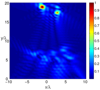
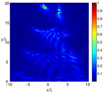
Figure 2. Migration images of $\eta^{(1)}$ (left) and $\eta^{(2)}$ (right) in a homogeneous medium.

Migration images of $\eta_{1}$ and $\eta_{2}$ in a homogeneous medium are shown in Figure 2. They peak at the scatterer locations. We observe that the resolution of the images is of the order of the wavelength. Since this is smaller for the second harmonic, the resolution of the image of $\eta_{2}$ is better.

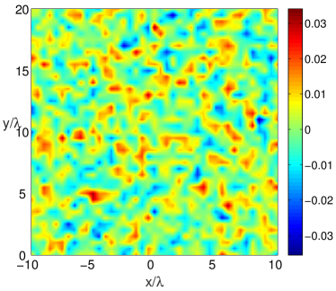
Figure 3. One realization of the process $\mu$.

We study imaging in a random medium, generated numerically with random Fourier series [31] for the Gaussian autocorrelation function (3.2) with correlation length $\ell=0.3\lambda$, and standard deviation $\sigma=0.01\times(4\pi)$. We display in Figure 3 one realization of $\eta$. The migration and CINT images of $\eta_{1}$ and $\eta_{2}$ in a small search region near the scatterer are shown in Figures  4 and 5, for two realizations of the random medium. The thresholding parameters in the CINT image formation are $X_{1}=2X_{2}=7\lambda$ and $\Theta={\pi}/{5}$. We observe that as predicted by the theory in section 3, the migration images change significantly from one realization to another, whereas CINT images of $\eta_{1}$ and $\eta_{2}$ are almost the same and peak near the scatters. The figures also show that the CINT images are blurrier than those in homogeneous media displayed in Figure 2.

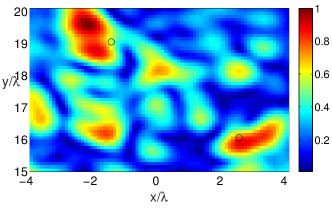
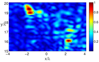
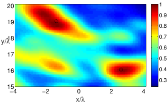
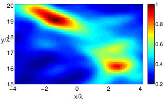
Figure 4. The migration (top row) and CINT (bottom) row images of the linear susceptibility $\eta_{1}$ in two realizations of the random medium. The scatterer location is shown with a black circle.

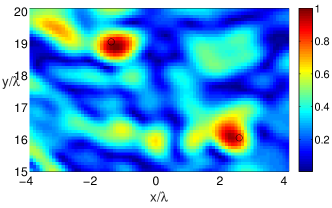
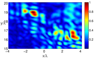
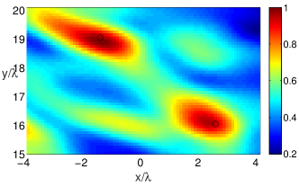
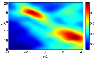
Figure 5. The migration (top row) and CINT (bottom) row images of the quadratic susceptibility $\eta_{2}$ in two realizations of the random medium. The scatterer location is shown by a black circle.

The images of the quadratic susceptibility, displayed in Figure 5 are similar to those of the linear susceptibility, shown in Figure 5. This is because we limited the search domain to the vicinity of the scatterer, and as predicted by the theory in section 3, the uncompensated incident waves in the array data do not have an effect far from the array. However, as shown in Figure 6, these waves cause strong artifacts of the images of the linear susceptibility over larger imaging domains. The image of the quadratic susceptibility is not affected by the direct waves and is clearly better.

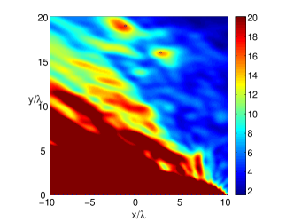
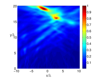
Figure 6. CINT images of the linear susceptibility (left) and quadratic susceptibility (right). Here we used 81 incident directions and 81 detectors.

5. Conclusions

We have investigated the problem of optical imaging of small scatterers with second-harmonic light in random media. We have found that the performance of CINT is superior to that of migration imaging. That is, images obtained by CINT are more robust to statistical fluctuations in the background medium. This observation is consistent with a resolution analysis that is carried out using a geometrical optics model for light propagation in random media. It is also in accord with numerical simulations for which the assumptions of the geometrical optics model do not hold.

Appendix A Statistical moments

In this appendix we calculate the statistical moments of the wave fields. We begin in section A.1 with the second moments of the random phases, which are approximately Gaussian distributed in our scaling regime described in section 3.1. Then we calculate the second moments of the wave fields in section A.2.

A.1. Moments of the random phases

We establish first the following result: Let $\bm{x},\bm{x}^{\prime}$ be two points in the set $\mathbb{A}$ defined in (3.3). The second moments of the processes (3.14) and (3.16) are approximated by

$$\mathbb{E}[\nu(\bm{x},\bm{y})\nu(\bm{x}^{\prime},\bm{y})]\approx\frac{\sqrt{2\pi}\sigma^{2}\ell|\bm{x}^{\prime}-\bm{y}|}{4}\int_{0}^{1}dt\,e^{-\frac{t^{2}}{2\ell^{2}}\left|\bm{x}^{\prime}_{\perp}-\bm{x}_{\perp}\right|^{2}},$$ (A.1)

and

$$\mathbb{E}[\gamma(\bm{x},{\bm{\theta}})\gamma(\bm{x}^{\prime},{\bm{\theta}}^{\prime})]\approx\frac{\sqrt{2\pi}\sigma^{2}\ell|\bm{x}^{\prime}-\bm{x}^{\prime(i)}({\bm{\theta}}^{\prime})|}{4}\int_{0}^{1}dt\,e^{-\frac{1}{2\ell^{2}}\left|\bm{P}_{\bm{\vartheta}}\left[(1-t)(\bm{x}^{\prime(i)}({\bm{\theta}}^{\prime})-\bm{x}^{(i)}({\bm{\theta}}))+t(\bm{x}^{\prime}-\bm{x})\right]\right|^{2}}.$$ (A.2)

The cross-moments satisfy

$$\left|\mathbb{E}[\gamma(\bm{x},{\bm{\theta}})\nu(\bm{x}^{\prime},\bm{y})]\right|\ll\lambda^{2},\quad\left|\mathbb{E}[\gamma(\bm{y},{\bm{\theta}})\nu(\bm{x}^{\prime},\bm{y})]\right|\ll\lambda^{2}.$$ (A.3)

To derive equation (A.1), we use (3.14) and the Gaussian autocorrelation (3.2) to obtain

$$\mathbb{E}[\nu(\bm{x},\bm{y})\nu(\bm{x}^{\prime},\bm{y})] =\frac{\sigma^{2}|\bm{x}-\bm{y}||\bm{x}^{\prime}-\bm{y}|}{4}\int_{0}^{1}dt\int_{0}^{1}dt^{\prime}\,\mathbb{E}\left[\mu\left(\frac{(1-t)\bm{y}}{\ell}+\frac{t\bm{x}}{\ell}\right)\mu\left(\frac{(1-t^{\prime})\bm{y}}{\ell}+\frac{t^{\prime}\bm{x}^{\prime}}{\ell}\right)\right]$$

$$=\frac{\sigma^{2}|\bm{x}-\bm{y}||\bm{x}^{\prime}-\bm{y}|}{4}\int_{0}^{1}dt\int_{0}^{1}dt^{\prime}\,e^{-\frac{1}{2\ell^{2}}\left|(t^{\prime}-t)(\bm{x}-\bm{y})+t^{\prime}(\bm{x}^{\prime}-\bm{x})\right|^{2}},$$ (A.4)

for $\bm{x},\bm{x}^{\prime}\in A$. We change variables

$$(t,t^{\prime})\to(\widetilde{t},t^{\prime}),\quad\widetilde{t}=(t^{\prime}-t)|\bm{x}-\bm{y}|/\ell,$$

with $t^{\prime}\in(0,1)$ and $\widetilde{t}\in(-(1-t^{\prime})|\bm{x}-\bm{y}|/\ell,t^{\prime}|\bm{x}-\bm{y}|/\ell)$, and use that $|\bm{x}-\bm{y}|/\ell\approx L/\ell\gg 1$ to extend the $\widetilde{t}$ integral to the real line. We obtain

$$\mathbb{E}[\nu(\bm{x},\bm{y})\nu(\bm{x}^{\prime},\bm{y})]\approx\frac{\sqrt{2\pi}\ell|\bm{x}^{\prime}-\bm{y}|}{4}\int_{0}^{1}dt^{\prime}e^{-\frac{1}{2\ell^{2}}\left|t^{\prime}\bm{P}(\bm{x}^{\prime}-\bm{x})\right|^{2}},$$ (A.5)

where $\bm{P}$ is the orthogonal projection on the plane orthogonal to $\bm{x}-\bm{y}$. In our case we have

$$\left|\frac{\bm{x}-\bm{y}}{|\bm{x}-\bm{y}|}-\bm{n}\right|=O\left(\frac{a}{L}\right)\ll 1,$$ (A.6)

and we can estimate the projection in (A.5) by

$$\frac{\bm{P}(\bm{x}^{\prime}-\bm{x})}{\ell}=\frac{\bm{P}_{{}_{\bm{n}}}(\bm{x}^{\prime}-\bm{x})}{\ell}+O\left(\frac{a^{2}}{\ell L}\right),\quad\bm{P}_{n}=I-\bm{n}\bm{n}^{T}.$$ (A.7)

The residual in (3.5) is negligible by assumption (3.11), that gives

$$\frac{a^{2}}{\ell L}\ll\frac{\sqrt{\lambda L}}{\ell}\ll 1.$$

Equation (A.1) follows from (A.5) and (A.7).

The derivation of (A.2) is essentially the same, so let us calculate the cross-moments. We obtain from (3.14), (3.16) and the Gaussian autocorrelation (3.2) that

$$\mathbb{E}[\gamma(\bm{x},{\bm{\theta}})\nu(\bm{x}^{\prime},\bm{y})] =\frac{\sigma^{2}|\bm{x}-\bm{x}^{(i)}({\bm{\theta}})||\bm{x}^{\prime}-\bm{y}|}{4}\int_{0}^{1}dt\int_{0}^{1}dt^{\prime}\,e^{-\frac{1}{2}\big{|}\frac{t^{\prime}(\bm{x}-\bm{x}^{(i)}({\bm{\theta}}))}{\ell}+\frac{t(\bm{x}^{\prime}-\bm{y})}{\ell}+\frac{\bm{y}-\bm{x}}{\ell}\big{|}^{2}},$$ (A.8)

where the result is obviously positive, so no absolute value is needed. Changing variables

$$(t,t^{\prime})\to(T,T^{\prime}),\quad T=t\frac{|\bm{x}^{\prime}-\bm{y}|}{\ell},\quad T^{\prime}=t^{\prime}\frac{|\bm{x}-\bm{x}^{(i)}({\bm{\theta}})|}{\ell},$$

and extending the integrals to the real line, we obtain the upper bound

$$\mathbb{E}[\gamma(\bm{x},{\bm{\theta}})\nu(\bm{x}^{\prime},\bm{y})] \leq\frac{\sigma^{2}\ell^{2}}{4}\int_{-\infty}^{\infty}dT\int_{-\infty}^{\infty}dT^{\prime}\,e^{-\frac{1}{2}\left|T^{\prime}{\bm{\theta}}+T\frac{(\bm{x}^{\prime}-\bm{y})}{|\bm{x}^{\prime}-\bm{y}|}+\frac{\bm{y}-\bm{x}}{\ell}\right|^{2}}.$$ (A.9)

Expanding the square in the exponent,

$$\left|T^{\prime}{\bm{\theta}}+T\left(\frac{\bm{x}^{\prime}-\bm{y}}{|\bm{x}^{\prime}-\bm{y}|}\right)+\frac{\bm{y}-\bm{x}}{\ell}\right|^{2} =\left[T^{\prime}+T\frac{{\bm{\theta}}\cdot(\bm{x}^{\prime}-\bm{y})}{|\bm{x}^{\prime}-\bm{y}|}+\frac{{\bm{\theta}}\cdot(\bm{y}-\bm{x})}{\ell}\right]^{2}$$

$$+\left|\bm{P}_{{\bm{\theta}}}\left[T\frac{(\bm{x}^{\prime}-\bm{y})}{|\bm{x}^{\prime}-\bm{y}|}+\frac{\bm{y}-\bm{x}}{\ell}\right]\right|^{2}$$

with $\bm{P}_{{\bm{\theta}}}=I-{\bm{\theta}}{\bm{\theta}}^{T}$, we obtain after integrating in $T^{\prime}$ that

$$\mathbb{E}[\gamma(\bm{x},{\bm{\theta}})\nu(\bm{x}^{\prime},\bm{y})] \leq\frac{\sqrt{2\pi}\sigma^{2}\ell^{2}}{4}\int_{-\infty}^{\infty}dTe^{-\frac{1}{2}\left|\bm{P}_{{\bm{\theta}}}\left[T\frac{(\bm{x}^{\prime}-\bm{y})}{|\bm{x}^{\prime}-\bm{y}|}+\frac{\bm{y}-\bm{x}}{\ell}\right]\right|^{2}}.$$ (A.10)

To evaluate the $T$ integral we proceed similarly, by decomposing the vector $\bm{P}_{{\bm{\theta}}}(\bm{y}-\bm{x})$ in two parts: one along the vector $\bm{P}_{{\bm{\theta}}}(\bm{x}^{\prime}-\bm{y})$ and the other orthogonal to it. Then, we expand the square in (A.10) and obtain after integration in $T$ the upper bound

$$\mathbb{E}[\gamma(\bm{x},{\bm{\theta}})\nu(\bm{x}^{\prime},\bm{y})] \leq\frac{2\pi\sigma^{2}\ell^{2}}{4\left|\bm{P}_{{\bm{\theta}}}\frac{(\bm{x}^{\prime}-\bm{y})}{|\bm{x}^{\prime}-\bm{y}|}\right|}.$$ (A.11)

Equation (A.3) follows from the assumptions (3.8), $\bm{\vartheta}\perp\bm{n}$ and equation (A.7) which give

$$\left|\bm{P}_{{\bm{\theta}}}\frac{(\bm{x}^{\prime}-\bm{y})}{|\bm{x}^{\prime}-\bm{y}|}\right|=O(1),$$

so that the right hand side in (A.11) is $O(\sigma^{2}\ell^{2})$. But by assumption (3.12),

$$\sigma^{2}\ell^{2}\ll\frac{\lambda\ell^{3}}{L^{2}}\ll{\lambda^{2}},$$

with the last inequality implied by the upper bound on $\ell$ in (3.11).

A.2. Second moments of the wave fields

Let us suppose, without loss of generality, that

$$|\bm{x}-\bm{y}|\geq|\bm{x}^{\prime}-\bm{y}|,\quad|\bm{x}-\bm{x}^{(i)}({\bm{\theta}})|\geq|\bm{x}^{\prime}-\bm{x}^{\prime(i)}({\bm{\theta}}^{\prime})|,$$ (A.12)

and use the results of the preceding section to derive the second moments of the wave fields.

A.2.1. Derivation of moment formula (3.26):

Using that the phases are approximately Gaussian, we obtain

$$\mathbb{E}\left[G(\bm{x},\bm{y};j\omega){G^{\star}(\bm{x}^{\prime},\bm{y};j\omega)}\right]\approx G_{0}(\bm{x},\bm{y};j\omega){G_{0}^{\star}(\bm{x}^{\prime},\bm{y};j\omega)}$$

$$\times\exp\Big{\{}-\frac{(jk)^{2}}{2}\mathbb{E}\Big{[}\big{(}\nu(\bm{x},\bm{y})-\nu(\bm{x}^{\prime},\bm{y})\big{)}^{2}\Big{]}\Big{\}},$$ (A.13)

with exponent written using (A.1) and definition (3.23) as follows

$$\frac{(jk)^{2}}{2}\mathbb{E}\big{\{}\big{[}\nu(\bm{x},\bm{y})-\nu(\bm{x}^{\prime},\bm{y})\big{]}^{2}\big{\}}=\frac{|\bm{x}-\bm{y}|}{\ell_{j}^{s}}+\frac{|\bm{x}^{\prime}-\bm{y}|}{\ell_{j}^{s}}-\frac{2|\bm{x}^{\prime}-\bm{y}|}{\ell_{j}^{s}}\int_{0}^{1}dt\,\exp\Big{(}-\frac{t^{2}}{2\ell^{2}}\left|\bm{x}^{\prime}_{\perp}-\bm{x}_{\perp}\right|^{2}\Big{)}.$$

Since $|\bm{x}-\bm{y}|,|\bm{x}^{\prime}-\bm{y}|\approx L\gg\ell_{j}^{s}$, this is very large and therefore (A.13) is negligible, unless the integral is close to one. This happens when

$$\big{|}\bm{x}^{\prime}_{\perp}-\bm{x}_{\perp}\big{|}\ll\ell,$$ (A.14)

in which case we can use a Taylor expansion of the exponential and obtain the approximation

$$\int_{0}^{1}dt\,e^{-\frac{t^{2}}{2\ell^{2}}\left|\bm{x}^{\prime}_{\perp}-\bm{x}_{\perp}\right|^{2}}\approx 1-\frac{\big{|}\bm{x}^{\prime}_{\perp}-\bm{x}_{\perp}\big{|}^{2}}{6\ell^{2}}.$$

Substituting in (A.13), we get

$$\mathbb{E}\left[G(\bm{x},\bm{y};j\omega){G^{\star}(\bm{x}^{\prime},\bm{y};j\omega)}\right]\approx G_{0}(\bm{x},\bm{y};j\omega){G_{0}^{\star}(\bm{x}^{\prime},\bm{y};j\omega)}$$ (A.15)

$$\times\exp\Big{(}-\frac{\left||\bm{x}-\bm{y}|-|\bm{x}^{\prime}-\bm{y}|\right|}{\ell_{j}^{s}}-\frac{|\bm{x}^{\prime}_{\perp}-\bm{x}_{\perp}|^{2}}{2X_{d,j}^{2}}\Big{)},$$ (A.16)

with

$$X_{d,j}=\ell\sqrt{\frac{3\ell_{j}^{s}}{2|\bm{x}^{\prime}-\bm{y}|}}\approx\ell\sqrt{\frac{3\ell_{j}^{s}}{2L}}.$$ (A.17)

We also have

$$|\bm{x}-\bm{y}|-|\bm{x}^{\prime}-\bm{y}|\approx\frac{(\bm{x}-\bm{y})}{|\bm{x}-\bm{y}|}\cdot(\bm{x}-\bm{x}^{\prime})=\bm{n}\cdot(\bm{x}-\bm{x}^{\prime})+O\left(\frac{a^{2}}{L}\right)=O\left(\frac{a^{2}}{L}\right),$$ (A.18)

where we used (A.6) and that the array aperture is orthogonal to $\bm{n}$. But definition (3.23) of $\ell_{j}^{s}$ and assumptions (3.11)-(3.12) give

$$\frac{\left||\bm{x}-\bm{y}|-|\bm{x}^{\prime}-\bm{y}|\right|}{\ell_{j}^{s}}=O\left(\frac{a^{2}}{L\ell_{j}^{s}}\right)=O\left(\frac{a^{2}\ell\sigma^{2}}{L\lambda^{2}}\right)\ll\frac{a^{2}\ell^{2}}{\lambda L^{3}}\ll\frac{a^{4}}{\lambda L^{3}}\ll 1,$$ (A.19)

so the first term in the exponent of (A.16) is negligible. Equation (3.26) follows from (A.16), (A.18) and the paraxial approximation (3.10) of $G_{0}$. This formula is derived under assumption (A.14). If this doesn’t hold, the moment is exponentially small, of the order $\exp(-2L/\ell_{j}^{s})$, as explained above. This is captured in the expression (A.18) by the exponential decay on the scale $X_{d,j}$, which is much smaller than $\ell$ because $\ell_{j}^{s}\ll L$.

A.2.2. Derivation of moment formula (3.28):

Again, using the approximate Gaussian nature of the phases, we obtain from definition (3.15) that

$$\mathbb{E}\left[u_{1}^{(i)}(\bm{x},{\bm{\theta}}){u_{1}^{(i)}(\bm{x}^{\prime},{\bm{\theta}}^{\prime})}^{*}\right]\approx\exp\Big{\{}ik(\bm{x}\cdot{\bm{\theta}}-\bm{x}^{\prime}\cdot{\bm{\theta}}^{\prime})-\frac{k^{2}}{2}\mathbb{E}\Big{[}\left(\gamma(\bm{x},{\bm{\theta}})-\gamma(\bm{x}^{\prime},{\bm{\theta}}^{\prime})\right)^{2}\Big{]}\Big{\}},$$ (A.20)

with the last term in the exponent following from (A.2)

$$\frac{k^{2}}{2}\mathbb{E}\left\{\left[\gamma(\bm{x},{\bm{\theta}})-\gamma(\bm{x}^{\prime},{\bm{\theta}}^{\prime})\right]^{2}\right\}\approx\frac{|\bm{x}-\bm{x}^{(i)}({\bm{\theta}})|}{\ell_{j}^{s}}+\frac{|\bm{x}^{\prime}-\bm{x}^{\prime(i)}({\bm{\theta}}^{\prime})|}{\ell_{j}^{s}}-\frac{2|\bm{x}^{\prime}-\bm{x}^{\prime(i)}({\bm{\theta}}^{\prime})|}{\ell_{j}^{s}}$$

$$\times\int_{0}^{1}dt\,\exp\Big{[}-\frac{1}{2\ell^{2}}\left|\bm{P}_{\bm{\vartheta}}\left[(1-t)(\bm{x}^{\prime(i)}({\bm{\theta}}^{\prime})-\bm{x}^{(i)}({\bm{\theta}}))+t(\bm{x}^{\prime}-\bm{x})\right]\right|^{2}\Big{]}.$$ (A.21)

We conclude as above that since $|\bm{x}-\bm{x}^{(i)}({\bm{\theta}})|,|\bm{x}^{\prime}-\bm{x}^{\prime(i)}({\bm{\theta}})|\gg\ell_{j}^{s}$, the right hand side in (A.20) is small unless

$$\frac{|\bm{P}_{\bm{\vartheta}}(\bm{x}^{\prime}-\bm{x})|}{\ell}\ll 1,\quad\frac{|\bm{P}_{\bm{\vartheta}}(\bm{x}^{\prime(i)}({\bm{\theta}}^{\prime})-\bm{x}^{(i)}({\bm{\theta}}))|}{\ell}\ll 1.$$ (A.22)

By definition

$$\bm{x}^{(i)}({\bm{\theta}})=\bm{x}-|\bm{x}-\bm{x}^{(i)}({\bm{\theta}})|{\bm{\theta}},\quad\bm{x}^{\prime(i)}({\bm{\theta}}^{\prime})=\bm{x}^{\prime}-|\bm{x}^{\prime}-\bm{x}^{\prime(i)}({\bm{\theta}}^{\prime})|{\bm{\theta}}^{\prime},$$ (A.23)

so the last inequality in (A.22) implies that the angle between ${\bm{\theta}}$ and ${\bm{\theta}}^{\prime}$ must be small.

With the assumption (A.22), we can approximate the integral using the Taylor expansion of the exponential,

$$\exp\Big{\{}-\frac{k^{2}}{2}\mathbb{E}\Big{[}\Big{(}\gamma(\bm{x},{\bm{\theta}})-\gamma(\bm{x}^{\prime},{\bm{\theta}}^{\prime})\Big{)}^{2}\Big{]}\Big{\}}\approx\exp\left[-\frac{\left||\bm{x}-\bm{x}^{(i)}({\bm{\theta}})|-|\bm{x}^{\prime}-\bm{x}^{\prime(i)}({\bm{\theta}}^{\prime})|\right|}{\ell_{1}^{s}}\right.$$

$$\left.-\frac{|\bm{P}_{\bm{\vartheta}}\widetilde{\bm{x}}|^{2}+\widetilde{\bm{x}}\cdot\bm{P}_{\bm{\vartheta}}\widetilde{\bm{x}}^{(i)}+|\bm{P}_{\bm{\vartheta}}\widetilde{\bm{x}}^{(i)}|^{2}}{2X_{d,1}^{2}}\right],$$ (A.24)

with $\ell_{1}^{s}$ defined in (3.23), $X_{d,1}$ defined in (A.17), $\widetilde{\bm{x}}=\bm{x}-\bm{x}^{\prime},$ and $\widetilde{\bm{x}}^{(i)}=\bm{x}^{(i)}({\bm{\theta}})-\bm{x}^{\prime(i)}({\bm{\theta}}^{\prime}).$ The first term in the exponential in (A.24) is of the same order as in the estimate (A.19), and is negligible. The second term can be rewritten using (A.23), which gives

$$\widetilde{\bm{x}}^{(i)}=\widetilde{\bm{x}}-\left[|\bm{x}-\bm{x}^{(i)}({\bm{\theta}})|-|\bm{x}^{\prime}-\bm{x}^{\prime(i)}({\bm{\theta}}^{\prime})|\right]\overline{\bm{\theta}}-\Big{[}|\bm{x}-\bm{x}^{(i)}({\bm{\theta}})|+|\bm{x}^{\prime}-\bm{x}^{\prime(i)}({\bm{\theta}}^{\prime})|\Big{]}\frac{\widetilde{\bm{\theta}}}{2},$$ (A.25)

where $\overline{\bm{\theta}}=({{\bm{\theta}}+{\bm{\theta}}^{\prime}})/{2}$ and $\widetilde{\bm{\theta}}={\bm{\theta}}-{\bm{\theta}}^{\prime}.$ Note that

$$\frac{\left||\bm{x}-\bm{x}^{(i)}({\bm{\theta}})|-|\bm{x}^{\prime}-\bm{x}^{\prime(i)}({\bm{\theta}}^{\prime})|\right|}{X_{d,1}}=O\left(\frac{a^{2}}{LX_{d,1}}\right)=O\left(\frac{a^{2}\sigma}{\lambda\sqrt{\ell L}}\right)\ll\frac{a^{2}}{\sqrt{\lambda L^{3}}}\ll 1,$$

where we used the definition of $X_{d,1}$ and the scaling assumptions (3.11)-(3.12). Thus, we can neglect the second term in the right hand-side of (A.25), and get

$$\widetilde{\bm{x}}^{(i)}\approx\widetilde{\bm{x}}-|\bm{x}-\bm{x}^{(i)}({\bm{\theta}})|\widetilde{\bm{\theta}}.$$ (A.26)

Gathering the results and substituting in (A.20) and (A.24) we obtain (3.28).

A.2.3. Derivation of moment formula (3.32):

This follows from

$$\mathbb{E}\left[G(\bm{x},\bm{y};j\omega)e^{ijk\gamma(\bm{y},{\bm{\theta}})}\right] \approx G_{0}(\bm{x},\bm{y};j\omega)\exp\Big{\{}-\frac{(jk)^{2}}{2}\mathbb{E}\left[\left(\nu(\bm{x},\bm{y})-\gamma(\bm{y},{\bm{\theta}})\right)^{2}\right]\Big{\}}$$

$$\approx G_{0}(\bm{x},\bm{y};j\omega)\exp\left[-\frac{|\bm{x}-\bm{y}|}{\ell_{j}^{s}}-\frac{|\bm{y}-\bm{y}^{(i)}({\bm{\theta}})|}{\ell_{j}^{s}}\right],$$ (A.27)

where the first approximation is because the phases are approximately Gaussian, and the second approximation is because by (A.3),

$$k^{2}\left|\mathbb{E}\left[\nu(\bm{x},\bm{y})\gamma(\bm{y},{\bm{\theta}})\right]\right|\ll 1.$$ (A.28)

Appendix B Statistics of the migration image

To find the expectation $\mathbb{E}\big{[}\mathcal{I}^{{M}}_{{}_{j}}(\bm{y})\big{]}$ of the migration imaging function and evaluate the SNR, we use the following moment factorizations implied by (A.28),

$$\mathbb{E}\left[G(\bm{x},\bm{y};j\omega){G^{\star}(\bm{x}^{\prime},\bm{y};j\omega)}e^{ijk[\gamma(\bm{y},{\bm{\theta}})-\gamma(\bm{y},{\bm{\theta}}^{\prime})]}\right]\approx\mathbb{E}\left[G(\bm{x},\bm{y};j\omega){G^{\star}(\bm{x}^{\prime},\bm{y};j\omega)}\right]$$

$$\times\mathbb{E}\left[e^{ijk[\gamma(\bm{y},{\bm{\theta}})-\gamma(\bm{y},{\bm{\theta}}^{\prime})]}\right],$$ (B.1)

and

$$\mathbb{E}\left[{G^{\star}(\bm{x}^{\prime},\bm{y};j\omega)}e^{ijk[\gamma(\bm{y},{\bm{\theta}}^{\prime})-\gamma(\bm{x},{\bm{\theta}})]}\right]\approx\mathbb{E}\left[{G^{\star}(\bm{x}^{\prime},\bm{y};j\omega)}\right]\mathbb{E}\left[e^{ijk[\gamma(\bm{y},{\bm{\theta}}^{\prime})-\gamma(\bm{x},{\bm{\theta}})]}\right].$$ (B.2)

We analyze separately the imaging of the linear and quadratic susceptibilities.

B.1. Imaging of the linear susceptibility

Definitions (3.35) and (3.37), and the estimates (3.25), (3.32) give that the expectation of the image is

$$\mathbb{E}\left[\mathcal{I}^{{M}}_{{}_{1}}(\bm{y}^{R})\right]\approx-\int_{A}d\bm{x}_{\perp}\int_{C}d{\bm{\theta}}\,{G_{0}^{\star}(\bm{x},\bm{y}^{R};\omega)}\exp\Big{[}ik{\bm{\theta}}\cdot(\bm{x}-\bm{y}^{R})\Big{]}$$

$$+\int_{A}d\bm{x}_{\perp}\int_{C}d{\bm{\theta}}\,{G_{0}^{\star}(\bm{x},\bm{y}^{R};\omega)}\exp\Big{[}ik{\bm{\theta}}\cdot(\bm{x}-\bm{y}^{R})-\frac{|\bm{x}-\bm{x}^{(i)}({\bm{\theta}})|}{\ell_{1}^{s}}\Big{]}$$

$$+k^{2}\left<\eta_{1}\right>\int_{A}d\bm{x}_{\perp}\int_{C}d{\bm{\theta}}\,G_{0}(\bm{x},\bm{y};\omega){G_{0}^{\star}(\bm{x},\bm{y}^{R};\omega)}\exp\Big{[}ik{\bm{\theta}}\cdot(\bm{y}-\bm{y}^{R})-\frac{(|\bm{x}-\bm{y}|+|\bm{y}-\bm{y}^{(i)}({\bm{\theta}})|)}{\ell_{1}^{s}}\Big{]}.$$ (B.3)

All the terms but the first in this expression are exponentially small. But even this term gives a small contribution because of the large phase

$$k\left[|\bm{x}-\bm{y}^{R}|-{\bm{\theta}}\cdot(\bm{x}-\bm{y}^{R})\right]=k|\bm{x}-\bm{y}^{R}|\left[1-{\bm{\theta}}\cdot\frac{(\bm{x}-\bm{y}^{R})}{|\bm{x}-\bm{y}^{R}|}\right]=O(L/\lambda)\gg 1,$$

where we used the expression of $G_{0}(\bm{x},\bm{y}^{R},\omega)$ and that $\bm{\vartheta}\perp\bm{n}$.

The second moment of the imaging function at the scatterer location is

$$\mathbb{E}\left[\left|\mathcal{I}^{{M}}_{{}_{1}}(\bm{y})\right|^{2}\right] \approx\int_{A}d\bm{x}_{\perp}\int_{A}d\bm{x}^{\prime}_{\perp}\int_{C}d{\bm{\theta}}\int_{C}d{\bm{\theta}}^{\prime}\,G_{0}(\bm{x}^{\prime},\bm{y};\omega){G_{0}^{\star}(\bm{x},\bm{y};\omega)}$$

$$\times\Big{\{}\exp\Big{[}ik\Big{(}{\bm{\theta}}\cdot\bm{x}-{\bm{\theta}}^{\prime}\cdot\bm{x}^{\prime}-\bm{y}\cdot({\bm{\theta}}-{\bm{\theta}}^{\prime})\Big{)}\Big{]}\left[\mathbb{E}\left[\exp\Big{(}ik[\gamma(\bm{x},{\bm{\theta}})-\gamma(\bm{x}^{\prime},{\bm{\theta}}^{\prime})]\Big{)}\right]+1\right]$$

$$+(k^{2}\left<\eta_{1}\right>)^{2}\mathbb{E}\left[G(\bm{x},\bm{y};\omega){G^{\star}(\bm{x}^{\prime},\bm{y};\omega)}\right]\mathbb{E}\left[\exp\Big{(}ik(\gamma(\bm{y},{\bm{\theta}})-\gamma(\bm{y},{\bm{\theta}}^{\prime}))\Big{)}\right]\Big{\}},$$

where we dropped all the exponentially small terms. Using (3.26) and (3.28), we see that the result is clearly much larger than the square of (B.3). Thus, the standard deviation of the image

$$\mbox{std}[\mathcal{I}^{{M}}_{{}_{1}}(\bm{y})]=\sqrt{\mathbb{E}\left[\left|\mathcal{I}^{{M}}_{{}_{1}}(\bm{y})\right|^{2}\right]-\left|\mathbb{E}\left[\mathcal{I}^{{M}}_{{}_{1}}(\bm{y})\right]\right|^{2}}\approx\sqrt{\mathbb{E}\left[\left|\mathcal{I}^{{M}}_{{}_{1}}(\bm{y})\right|^{2}\right]}$$

is much larger than its mean. This gives the small SNR in equation (3.42).

B.2. Imaging of the quadratic susceptibility

We obtain similarly from definitions (3.36) and (3.37), and the estimates (3.25) and (3.32) that

$$\mathbb{E}\left[\mathcal{I}^{{M}}_{{}_{2}}(\bm{y}^{R})\right] \approx 4k^{2}\left<\eta_{2}\right>\int_{A}d\bm{x}_{\perp}\int_{C}d{\bm{\theta}}\,G_{0}(\bm{x},\bm{y};2\omega){G_{0}^{\star}(\bm{x},\bm{y}^{R};2\omega)}$$

$$\exp\left[i2k{\bm{\theta}}\cdot(\bm{y}-\bm{y}^{R})-\frac{(|\bm{x}-\bm{y}|+|\bm{y}-\bm{y}^{(i)}({\bm{\theta}})|)}{\ell_{2}^{s}}\right].$$ (B.4)

This peaks at $\bm{y}^{R}=\bm{y}$, where the phase cancells out, but the peak there is small due to the decaying exponential, because $|\bm{x}-\bm{y}|$ and $|\bm{y}-\bm{y}^{(i)}({\bm{\theta}})|$ are much larger than the scattering length $\ell_{2}^{s}$. The second moment at the scatterer location is

$$\mathbb{E}\left[\left|\mathcal{I}^{{M}}_{{}_{2}}(\bm{y})\right|^{2}\right]\approx\big{(}4k^{2}\left<\eta_{2}\right>\big{)}^{2}\int_{A}d\bm{x}_{\perp}\int_{A}d\bm{x}^{\prime}_{\perp}\int_{C}d{\bm{\theta}}\int_{C}d{\bm{\theta}}^{\prime}\,G_{0}(\bm{x}^{\prime},\bm{y};2\omega){G_{0}^{\star}(\bm{x},\bm{y};2\omega)}$$

$$\times\mathbb{E}\left[G(\bm{x},\bm{y};2\omega){G^{\star}(\bm{x}^{\prime},\bm{y};2\omega)}\right]\mathbb{E}\left[\exp\Big{(}i2k(\gamma(\bm{y},{\bm{\theta}})-\gamma(\bm{y},{\bm{\theta}}^{\prime}))\Big{)}\right],$$ (B.5)

with the expectations in the second line calculated in appendix A.2. These expectations are large for nearby points in the array and nearby directions of illumination. Substituting in (B.5) and comparing with (B.4) leads us to

$$\mbox{std}[\mathcal{I}^{{M}}_{{}_{2}}(\bm{y})]=\sqrt{\mathbb{E}\left[\left|\mathcal{I}^{{M}}_{{}_{2}}(\bm{y})\right|^{2}\right]-\left|\mathbb{E}\left[\mathcal{I}^{{M}}_{{}_{2}}(\bm{y})\right]\right|^{2}}\approx\sqrt{\mathbb{E}\left[\left|\mathcal{I}^{{M}}_{{}_{2}}(\bm{y})\right|^{2}\right]}.$$

This gives the small SNR in equation (3.42).

Appendix C Statistics of the CINT image

We calculate here the mean and variance of the CINT imaging functions $\mathcal{I}^{{CINT}}_{{}_{j}}$, for $j=1,2$. The expression of the mean is needed to quantify the focusing of the image, and the variance is needed to assess the robustness with respect to different realizations of the random medium.

C.1. CINT image of the quadratic susceptibility

The expression of the CINT imaging function is obtained by substituting (3.51) in (3.52)

$$\mathcal{I}^{{CINT}}_{{}_{2}}(\bm{y}^{R}) =(4k^{2}\left<\eta_{2}\right>)^{2}\times\iint_{\mathcal{C}}d{\bm{\theta}}d\widetilde{\bm{\theta}}\,\exp\Big{\{}-\frac{|\bm{P}_{\bm{\vartheta}}\widetilde{\bm{\theta}}|^{2}}{2\Theta^{2}}+i2k[\gamma(\bm{y},{\bm{\theta}}+\widetilde{\bm{\theta}}/2)-\gamma(\bm{y},{\bm{\theta}}-\widetilde{\bm{\theta}}/2)]\Big{\}}$$

$$\times\exp\Big{\{}i2k[({\bm{\theta}}+\widetilde{\bm{\theta}}/2)\cdot(\bm{y}-\bm{y}^{R})-({\bm{\theta}}-\widetilde{\bm{\theta}}/2)\cdot(\bm{y}-\bm{y}^{R})]\Big{\}}$$

$$\times\iint_{A}d\bm{x}_{\perp}d\widetilde{\bm{x}}_{\perp}\,\exp\Big{(}-\frac{|\widetilde{\bm{x}}_{\perp}|^{2}}{2X^{2}}\Big{)}G\Big{(}\bm{x}+\frac{\widetilde{\bm{x}}}{2},\bm{y};2\omega\Big{)}G^{\star}\Big{(}\bm{x}-\frac{\widetilde{\bm{x}}}{2},\bm{y};2\omega\Big{)}$$

$$\times G_{0}^{\star}\Big{(}\bm{x}+\frac{\widetilde{\bm{x}}}{2},\bm{y}^{R};2\omega\Big{)}G_{0}\Big{(}\bm{x}-\frac{\widetilde{\bm{x}}}{2},\bm{y}^{R};2\omega\Big{)}\,.$$ (C.1)

It is given by the product of the integrals over the direction vectors and the detector coordinates. Because of the statistical decorrelation stated in (3.32) (see also the estimate (A.28)) we can study separately the statistics of these integrals, denoted by

$$\mathcal{J}_{\mathcal{A}}(\bm{y}^{R})= \iint_{\mathcal{A}}d\bm{x}_{\perp}d\widetilde{\bm{x}}_{\perp}e^{-\frac{|\widetilde{\bm{x}}_{\perp}|^{2}}{2X^{2}}}G\Big{(}\bm{x}+\frac{\widetilde{\bm{x}}}{2},\bm{y};2\omega\Big{)}G^{\star}\Big{(}\bm{x}-\frac{\widetilde{\bm{x}}}{2},\bm{y};2\omega\Big{)}G_{0}^{\star}\Big{(}\bm{x}+\frac{\widetilde{\bm{x}}}{2},\bm{y}^{R};2\omega\Big{)}$$

$$\times G_{0}\Big{(}\bm{x}-\frac{\widetilde{\bm{x}}}{2},\bm{y}^{R};2\omega\Big{)},$$ (C.2)

and

$$\mathcal{J}_{\mathcal{C}}(\bm{y}^{R})=\iint_{\mathcal{C}}d{\bm{\theta}}d\widetilde{\bm{\theta}}_{\perp}\,e^{-\frac{|\bm{P}_{\bm{\vartheta}}\widetilde{\bm{\theta}}|^{2}}{2\Theta^{2}}+i2k[({\bm{\theta}}+\widetilde{\bm{\theta}}/2)\cdot(\bm{y}-\bm{y}^{R})-({\bm{\theta}}-\widetilde{\bm{\theta}}/2)\cdot(\bm{y}-\bm{y}^{R})]+i2k[\gamma(\bm{y},{\bm{\theta}}+\widetilde{\bm{\theta}}/2)-\gamma(\bm{y},{\bm{\theta}}-\widetilde{\bm{\theta}}/2)]}.$$ (C.3)

C.1.1. Expectation of the imaging function

The integral $\mathcal{J}_{A}(\bm{y}^{R})$ models the CINT point spread function for a source at $\bm{y}$, and has been studied in [27]. Its expectation follows easily from (3.26) and the definition (3.44) of the set $\mathcal{A}$,

$$\mathbb{E}\left[\mathcal{J}_{A}(\bm{y}^{R})\right] \approx\frac{1}{L^{4}}\int_{A}d\bm{x}_{\perp}\int_{\mathbb{R}^{2}}d\widetilde{\bm{x}}_{\perp}\exp\Big{[}-\frac{|\widetilde{\bm{x}}_{\perp}|^{2}}{2X^{2}_{e}}+i2k\widetilde{\bm{x}}_{\perp}\cdot(\bm{y}^{R}_{\perp}-\bm{y}_{\perp})\Big{]}$$ (C.4)

$$\approx\frac{2\pi a^{2}X_{e}^{2}}{L^{4}}\exp\Big{[}-\frac{1}{2}\left(\frac{2kX_{e}|\bm{y}_{\perp}-\bm{y}^{R}_{\perp}|}{L}\right)^{2}\Big{]}.$$ (C.5)

Here we extended the $\widetilde{\bm{x}}_{\perp}$ integral to the whole plane using that $X_{e}\sim X_{d,2}\ll a$. Similarly, using (3.28) we get

$$\mathbb{E}\left[\mathcal{J}_{C}(\bm{y}^{R})\right]\approx\iint_{\mathcal{C}}d{\bm{\theta}}d\widetilde{\bm{\theta}}_{\perp}\,\exp\left[-\frac{|\bm{P}_{\bm{\vartheta}}\widetilde{\bm{\theta}}|^{2}}{2\Theta^{2}_{e}}+i2k\widetilde{\bm{\theta}}\cdot(\bm{y}-\bm{y}^{R})\right]$$

$$\hskip 14.45377pt=\iint_{\mathcal{C}}d{\bm{\theta}}d\widetilde{\bm{\theta}}_{\perp}\,\exp\left[-\frac{\big{(}\widetilde{\theta}_{\xi}^{2}+\widetilde{\theta}_{\zeta}^{2}\big{)}}{2\Theta_{e}^{2}}+i2k\widetilde{\theta}_{\zeta}{\bm{\zeta}}\cdot(\bm{y}-\bm{y}^{R})+2ik\widetilde{\theta}_{\xi}\big{(}{\bm{\xi}}-\tan\varphi\bm{\vartheta}\big{)}\cdot(\bm{y}-\bm{y}^{R})\right]$$ (C.6)

with $\widetilde{\theta}_{\xi}$, $\widetilde{\theta}_{\zeta}$, $\varphi$ parametrizing ${\bm{\theta}}$ and $\widetilde{\bm{\theta}}$ as in equations (3.45)–(3.50). To write the integral over the set $\mathcal{C}$, we recall from (3.45) and (3.49) that

$${\bm{\theta}}=\bm{\vartheta}\cos\varphi+{\bm{\xi}}(\beta)\sin\varphi+O(\Theta_{d}^{2}),$$

with azimuthal angle $\beta$ parametrizing the vectors ${\bm{\xi}}(\beta)$ and ${\bm{\zeta}}(\beta)$. In the calculation of the Jacobian of the transformation we may neglect the residual in this equation, and obtain

$$d{\bm{\theta}}=\sin\varphi d\varphi d\beta.$$

We also see from equation (3.50) that for any given $\varphi$ and $\beta$ we have, using $\varphi=O(\alpha)=O(a/L)\ll 1$, that

$$\partial_{\widetilde{\theta_{\xi}}}\widetilde{\bm{\theta}}\approx{\bm{\xi}}(\beta)\quad\mbox{and}\quad\partial_{\widetilde{\theta_{\zeta}}}\widetilde{\bm{\theta}}={\bm{\zeta}}(\beta),$$

and since ${\bm{\xi}}(\beta)$ and ${\bm{\zeta}}(\beta)$ are orthonormal, we get

$$d\widetilde{\bm{\theta}}=d\widetilde{\theta}_{\xi}d\widetilde{\theta}_{\zeta}.$$

The integrals over $\widetilde{\theta}_{\xi}$ and $\widetilde{\theta}_{\zeta}$ may be extended to the real line, because the Gaussians are negligible outside $\mathcal{C}$, and the result is

$$\mathbb{E}\left[\mathcal{J}_{C}(\bm{y}^{R})\right]\approx 2\pi\Theta_{e}^{2}\int_{0}^{\alpha}d\varphi\,\sin\varphi\int_{0}^{2\pi}d\beta\,\exp\Big{[}-\frac{(2k\Theta_{e})^{2}}{2}\big{[}(\bm{y}-\bm{y}^{R})\cdot{\bm{\zeta}}(\beta)\big{]}^{2}\Big{]}$$

$$\times\exp\Big{\{}-\frac{(2k\Theta_{e})^{2}}{2}\big{[}(\bm{y}-\bm{y}^{R})\cdot{\bm{\xi}}(\beta)-\tan\varphi(\bm{y}-\bm{y}^{R})\cdot\bm{\vartheta}\big{]}^{2}\Big{\}}.$$ (C.7)

We are interested only in the points $\bm{y}^{R}$ for which $\mathcal{J}_{\mathcal{A}}(\bm{y}^{R})$ is large, so

$$|(\bm{y}-\bm{y}^{R})\cdot\bm{\vartheta}|=O\left(\frac{L}{kX_{e}}\right).$$

Since $\Theta_{e}\approx X_{e}/L$ and $\varphi\leq\alpha\ll 1$, we have

$$k\Theta_{e}\tan\varphi|(\bm{y}-\bm{y}^{R})\cdot\bm{\vartheta}|\leq O(\alpha)\ll 1,$$

and we can neglect the $\varphi$ dependent term in the exponential in (C.7). We also note that

$$\big{[}(\bm{y}-\bm{y}^{R})\cdot{\bm{\zeta}}(\beta)\big{]}^{2}+\big{[}(\bm{y}-\bm{y}^{R})\cdot{\bm{\xi}}(\beta)\big{]}^{2}=\big{|}\bm{P}_{\bm{\vartheta}}(\bm{y}-\bm{y}^{R})\big{|}^{2}$$

is independent of $\beta$, so we obtain

$$\mathbb{E}\left[\mathcal{J}_{C}(\bm{y}^{R})\right] \approx 2\pi\Theta_{e}^{2}\exp\Big{\{}-\frac{\big{[}2k\Theta_{e}\big{|}\bm{P}_{\bm{\vartheta}}(\bm{y}-\bm{y}^{R})\big{|}\big{]}^{2}}{2}\Big{\}}\int_{0}^{\alpha}d\varphi\,\sin\varphi\int_{0}^{2\pi}d\beta$$

$$=2\pi^{2}\Theta_{e}^{2}\alpha^{2}\exp\Big{\{}-\frac{\big{[}2k\Theta_{e}\big{|}\bm{P}_{\bm{\vartheta}}(\bm{y}-\bm{y}^{R})\big{|}\big{]}^{2}}{2}\Big{\}}.$$ (C.8)

C.1.2. Variance of the imaging function

The variance of $\mathcal{J}_{A}$ is calculated in [27, Appendix E], so we revisit here the main ideas. The calculation involves the fourth moments of the Green’s function (3.13), which are determined by

$$\mathbb{E}\Big{\{}\exp\Big{[}i2k\big{[}\nu\big{(}\bm{x}+\frac{\widetilde{\bm{x}}}{2},\bm{y}\big{)}-\nu\big{(}\bm{x}-\frac{\widetilde{\bm{x}}}{2},\bm{y}\big{)}-\nu\big{(}\bm{x}^{\prime}+\frac{\widetilde{\bm{x}}^{\prime}}{2},\bm{y}\big{)}+\nu\big{(}\bm{x}^{\prime}-\frac{\widetilde{\bm{x}}^{\prime}}{2},\bm{y}\big{)}\big{]}\Big{]}\Big{\}}\approx e^{-\tau/2},$$ (C.9)

where we introduced the notation

$$\tau=(2k)^{2}\mathbb{E}\big{\{}\big{[}\nu\big{(}\bm{x}+\frac{\widetilde{\bm{x}}}{2},\bm{y}\big{)}-\nu\big{(}\bm{x}-\frac{\widetilde{\bm{x}}}{2},\bm{y}\big{)}-\nu\big{(}\bm{x}^{\prime}+\frac{\widetilde{\bm{x}}^{\prime}}{2},\bm{y}\big{)}+\nu\big{(}\bm{x}^{\prime}-\frac{\widetilde{\bm{x}}^{\prime}}{2},\bm{y}\big{)}\big{]}^{2}\big{\}},$$ (C.10)

and used the approximate Gaussian distribution of the phases. We need the second moments (A.1), rewritten as

$$(2k)^{2}\mathbb{E}\left[\nu(\bm{x},\bm{y})\nu(\bm{x}^{\prime},\bm{y})\right]=\frac{3\ell^{2}}{X_{d,2}^{2}}{h}\left(\frac{|\bm{x}_{\perp}-\bm{x}^{\prime}_{\perp}|}{\ell}\right),\quad{h}(z)=\frac{1}{z}\int_{0}^{z}dt\,e^{-\frac{t^{2}}{2}},$$ (C.11)

using the definition (3.27) of the decoherence length. The expression (C.10) becomes

$$\tau=\frac{6\ell^{2}}{X_{d,2}^{2}}\left[2-h\Big{(}\frac{\widetilde{\bm{x}}_{\perp}}{\ell}\Big{)}-h\Big{(}\frac{\widetilde{\bm{x}}^{\prime}_{\perp}}{\ell}\Big{)}+h\Big{(}\frac{\bm{x}_{\perp}-\bm{x}^{\prime}_{\perp}}{\ell}+\frac{\widetilde{\bm{x}}_{\perp}+\widetilde{\bm{x}}^{\prime}_{\perp}}{2\ell}\Big{)}+h\Big{(}\frac{\bm{x}_{\perp}-\bm{x}^{\prime}_{\perp}}{\ell}-\frac{\widetilde{\bm{x}}_{\perp}+\widetilde{\bm{x}}^{\prime}_{\perp}}{2\ell}\Big{)}\right.$$

$$\left.-h\Big{(}\frac{\bm{x}_{\perp}-\bm{x}^{\prime}_{\perp}}{\ell}+\frac{\widetilde{\bm{x}}_{\perp}-\widetilde{\bm{x}}^{\prime}_{\perp}}{2\ell}\Big{)}-h\Big{(}\frac{\bm{x}_{\perp}-\bm{x}^{\prime}_{\perp}}{\ell}-\frac{\widetilde{\bm{x}}_{\perp}-\widetilde{\bm{x}}^{\prime}_{\perp}}{2\ell}\Big{)}\right],$$

and we can simplify it because $|\widetilde{\bm{x}}_{\perp}|,|\widetilde{\bm{x}}^{\prime}_{\perp}|\lesssim X_{d,2}\ll\ell$, due to the windowing in the calculation of the cross-correlations. Expanding in $\widetilde{\bm{x}}_{\perp}/\ell$ and $\widetilde{\bm{x}}^{\prime}/\ell^{\prime}$ we get

$$\tau\approx\frac{6}{X_{d,2}^{2}}\left[\frac{|\widetilde{\bm{x}}_{\perp}|^{2}+|\widetilde{\bm{x}}^{\prime}_{\perp}|^{2}}{6}+\widetilde{\bm{x}}_{\perp}\cdot H\Big{(}\frac{\bm{x}_{\perp}-\bm{x}^{\prime}_{\perp}}{\ell}\Big{)}\widetilde{\bm{x}}^{\prime}_{\perp}\right],$$ (C.12)

where $H$ is the Hessian of $h$, evaluated at $(\bm{x}_{\perp}-\bm{x}^{\prime}_{\perp})/\ell$.

Because the Hessian decays, we note that the phase differences at points satisfying $|\bm{x}_{\perp}-\bm{x}^{\prime}_{\perp}|\gg\ell$ are decorrelated

$$\tau\approx\frac{|\widetilde{\bm{x}}_{\perp}|^{2}+|\widetilde{\bm{x}}^{\prime}_{\perp}|^{2}}{X_{d,2}^{2}}=(2k)^{2}\mathbb{E}\Big{\{}\Big{[}\nu\Big{(}\bm{x}+\frac{\widetilde{\bm{x}}}{2},\bm{y}\Big{)}-\nu\Big{(}\bm{x}-\frac{\widetilde{\bm{x}}}{2},\bm{y}\Big{)}\Big{]}^{2}\Big{\}}+(2k)^{2}\mathbb{E}\Big{\{}\Big{[}\nu\Big{(}\bm{x}^{\prime}+\frac{\widetilde{\bm{x}}^{\prime}}{2},\bm{y}\Big{)}$$

$$-\nu\Big{(}\bm{x}^{\prime}-\frac{\widetilde{\bm{x}}^{\prime}}{2},\bm{y}\Big{)}\Big{]}^{2}\Big{\}}.$$

It is only for $|\bm{x}_{\perp}-\bm{x}^{\prime}_{\perp}|\lesssim\ell$ that the Hessian contributes to (C.12). Thus, when calculating the variance of the CINT imaging function, we get a contribution only from the set of points

$$\{\bm{x},\bm{x}^{\prime}\in\mathbb{A},~{}~{}|\bm{x}_{\perp}-\bm{x}^{\prime}_{\perp}|\lesssim\ell\}.$$

This is why the SNR of $\mathcal{J}_{A}$ is of order $a/\ell$. We refer to [27, Appendix E] for more details.

The calculation of the variance of $\mathcal{J}_{C}$ is similar, and the SNR is of the same order.

C.2. CINT image of the linear susceptibility

The expression of the imaging function is obtained by substituting (3.56) in (3.57),

$$\mathcal{I}^{{CINT}}_{{}_{1}}(\bm{y}^{R})=\iint_{\mathcal{A}}d\bm{x}_{\perp}d\widetilde{\bm{x}}_{\perp}\iint_{\mathcal{C}}d{\bm{\theta}}d\widetilde{\bm{\theta}}\,e^{-\frac{|\widetilde{\bm{x}}_{\perp}|^{2}}{2X^{2}}-\frac{|\bm{P}_{\bm{\vartheta}}\widetilde{\bm{\theta}}|^{2}}{2\Theta^{2}}-ik\widetilde{\bm{\theta}}\cdot\bm{y}^{R}}G_{0}^{\star}\Big{(}\bm{x}+\frac{\widetilde{\bm{x}}}{2},\bm{y}^{R};\omega\Big{)}G_{0}\Big{(}\bm{x}-\frac{\widetilde{\bm{x}}}{2},\bm{y}^{R};\omega\Big{)}$$

$$\times\Big{\{}\Big{[}e^{-ik\gamma\big{(}\bm{x}-\frac{\widetilde{\bm{x}}}{2},{\bm{\theta}}-\frac{\widetilde{\bm{\theta}}}{2}\big{)}}-1\Big{]}e^{-ik\big{(}{\bm{\theta}}-\frac{\widetilde{\bm{\theta}}}{2}\big{)}\cdot\big{(}\bm{x}-\frac{\widetilde{\bm{x}}}{2}\big{)}}+k^{2}\left<\eta_{1}\right>G^{\star}\Big{(}\bm{x}-\frac{\widetilde{\bm{x}}}{2},\bm{y};\omega\Big{)}e^{-ik\big{(}{\bm{\theta}}-\frac{\widetilde{\bm{\theta}}}{2}\big{)}\cdot\bm{y}-ik\gamma\big{(}\bm{y},{\bm{\theta}}-\frac{\widetilde{\bm{\theta}}}{2}\big{)}}\Big{\}}$$

$$\times\Big{\{}\Big{[}e^{ik\gamma\big{(}\bm{x}+\frac{\widetilde{\bm{x}}}{2},{\bm{\theta}}+\frac{\widetilde{\bm{\theta}}}{2}\big{)}}-1\Big{]}e^{ik\big{(}{\bm{\theta}}+\frac{\widetilde{\bm{\theta}}}{2}\big{)}\cdot\big{(}\bm{x}+\frac{\widetilde{\bm{x}}}{2}\big{)}}+k^{2}\left<\eta_{1}\right>G\Big{(}\bm{x}+\frac{\widetilde{\bm{x}}}{2},\bm{y};\omega\Big{)}e^{ik\big{(}{\bm{\theta}}+\frac{\widetilde{\bm{\theta}}}{2}\big{)}\cdot\bm{y}+ik\gamma\big{(}\bm{y},{\bm{\theta}}+\frac{\widetilde{\bm{\theta}}}{2}\big{)}}\Big{\}}\,.$$ (C.13)

Using (3.26) and (3.28), we obtain the expectation

$$\mathbb{E} \Big{[}\mathcal{I}^{{CINT}}_{{}_{1}}(\bm{y}^{R})\Big{]}\approx\iint_{\mathcal{A}}d\bm{x}_{\perp}d\widetilde{\bm{x}}_{\perp}\iint_{\mathcal{C}}d{\bm{\theta}}d\widetilde{\bm{\theta}}\,e^{-\frac{|\widetilde{\bm{x}}_{\perp}|^{2}}{2X^{2}}-\frac{|\bm{P}_{\bm{\vartheta}}\widetilde{\bm{\theta}}|^{2}}{2\Theta^{2}}}G_{0}^{\star}\Big{(}\bm{x}+\frac{\widetilde{\bm{x}}}{2},\bm{y}^{R};\omega\Big{)}G_{0}\Big{(}\bm{x}-\frac{\widetilde{\bm{x}}}{2},\bm{y}^{R};\omega\Big{)}$$

$$\times e^{-ik\widetilde{\bm{\theta}}\cdot\bm{y}^{R}}\Big{\{}e^{ik{\bm{\theta}}\cdot\widetilde{\bm{x}}+ik\widetilde{\bm{\theta}}\cdot\bm{x}}\Big{[}\mathbb{E}\Big{[}e^{ik\big{[}\gamma\big{(}\bm{x}+\frac{\widetilde{\bm{x}}}{2},{\bm{\theta}}+\frac{\widetilde{\bm{\theta}}}{2}\big{)}-\gamma\big{(}\bm{x}+\frac{\widetilde{\bm{x}}}{2},{\bm{\theta}}+\frac{\widetilde{\bm{\theta}}}{2}\big{)}\big{]}}\Big{]}+1\Big{]}$$

$$+k^{4}\left<\eta_{1}\right>^{2}e^{ik\widetilde{\bm{\theta}}\cdot\bm{y}}\mathbb{E}\Big{[}G\Big{(}\bm{x}+\frac{\widetilde{\bm{x}}}{2},\bm{y};\omega\Big{)}G^{\star}\Big{(}\bm{x}-\frac{\widetilde{\bm{x}}}{2},\bm{y};\omega\Big{)}\Big{]}\mathbb{E}\Big{[}e^{ik\big{[}\gamma\big{(}\bm{y},{\bm{\theta}}+\frac{\widetilde{\bm{\theta}}}{2}\big{)}-\gamma\big{(}\bm{y},{\bm{\theta}}+\frac{\widetilde{\bm{\theta}}}{2}\big{)}\big{]}}\Big{]}\Big{\}},$$ (C.14)

where we have neglected the small terms due to decaying exponentials. We write the right hand side as the sum of three terms

$$\mathbb{E}\Big{[}\mathcal{I}^{{CINT}}_{{}_{1}}(\bm{y}^{R})\Big{]}\approx\mathcal{T}_{1}(\bm{y}^{R})+\mathcal{T}_{2}(\bm{y}^{R})+\mathcal{T}_{3}(\bm{y}^{R}).$$ (C.15)

The first two terms are due to the uncompensated incident wave, and are given by

$$\mathcal{T}_{1}(\bm{y}^{R})=\frac{1}{L^{2}}\iint_{\mathcal{A}}d\bm{x}_{\perp}d\widetilde{\bm{x}}_{\perp}\int_{\mathcal{C}}d{\bm{\theta}}{d}\widetilde{\bm{\theta}}\,\exp\Big{[}ik\widetilde{\bm{x}}\cdot{\bm{\theta}}-\frac{ik\widetilde{\bm{x}}_{\perp}\cdot(\bm{x}_{\perp}-\bm{y}^{R}_{\perp})}{L}+ik\widetilde{\bm{\theta}}\cdot(\bm{x}-\bm{y}^{R})\Big{]}$$

$$\times\exp\Big{[}-\frac{|\widetilde{\bm{x}}_{\perp}|^{2}}{2X^{2}}-\frac{|\bm{P}_{\bm{\vartheta}}\widetilde{\bm{\theta}}|^{2}}{2\Theta^{2}}\Big{]},$$ (C.16)

and

$$\mathcal{T}_{2}(\bm{y}^{R})=\frac{1}{L^{2}}\iint_{\mathcal{A}}d\bm{x}_{\perp}d\widetilde{\bm{x}}_{\perp}\int_{\mathcal{C}}d{\bm{\theta}}{d}\widetilde{\bm{\theta}}\,\exp\Big{[}ik\widetilde{\bm{x}}\cdot{\bm{\theta}}-\frac{ik\widetilde{\bm{x}}_{\perp}\cdot(\bm{x}_{\perp}-\bm{y}^{R}_{\perp})}{L}\big{)}+ik\widetilde{\bm{\theta}}\cdot(\bm{x}-\bm{y}^{R})\Big{]}$$

$$\times\exp\Big{[}-\frac{|\widetilde{\bm{x}}_{\perp}|^{2}}{2X^{2}}-\frac{|\bm{P}_{\bm{\vartheta}}\widetilde{\bm{\theta}}|^{2}}{2\Theta^{2}}-\frac{|\bm{P}_{\bm{\vartheta}}\widetilde{\bm{\theta}}|^{2}}{2[X_{d,1}/|\bm{x}-\bm{x}^{(i)}({\bm{\theta}})|]^{2}}-\frac{3}{2}\frac{|\bm{P}_{\bm{\vartheta}}\widetilde{\bm{x}}|^{2}}{X_{d,1}^{2}}+\frac{3}{2}\frac{\bm{P}_{\bm{\vartheta}}\widetilde{\bm{x}}}{X_{d,1}}\cdot\frac{\bm{P}_{\bm{\vartheta}}\widetilde{\bm{\theta}}}{X_{d,1}/|\bm{x}-\bm{x}^{(i)}({\bm{\theta}})|}\Big{]}.$$ (C.17)

Here we used the paraxial approximation (3.10) and moment formula (3.28). The third term is similar to the expectation of the imaging function for the quadratic susceptibility $\mathbb{E}[\mathcal{I}^{{CINT}}_{{}_{2}}(\bm{y}^{R})]$, so we write it directly,

$$\mathcal{T}_{3}(\bm{y}^{R})=\frac{(2\pi)^{3}}{2}\Big{(}k^{2}\left<\eta_{1}\right>^{2}\alpha\Theta_{e}\frac{aX_{e}}{L^{2}}\Big{)}^{2}\exp\Big{[}-\frac{1}{2}\left(\frac{kX_{e}|\bm{y}_{\perp}-\bm{y}^{R}_{\perp}|}{L}\right)^{2}-\frac{1}{2}\left(k\Theta_{e}|\bm{P}_{\bm{\vartheta}}(\bm{y}-\bm{y}^{R})|\right)^{2}\Big{]}.$$ (C.18)

To calculate (C.16) we recall the definition (3.44) of the set $\mathcal{A}$ and the parametrization of the set $\mathcal{C}$ described in equations (3.45)-(3.50). We integrate over $\widetilde{\bm{x}}_{\perp}$ using that $\widetilde{\bm{x}}$ is orthogonal to $\bm{n}$, and

$$k\widetilde{\bm{x}}\cdot{\bm{\theta}}=k|{\bm{\theta}}|\widetilde{\bm{x}}\cdot(\cos\varphi\,\bm{\vartheta}+\sin\varphi\,{\bm{\xi}}(\beta))=k\widetilde{\bm{x}}_{\perp}(\cos\varphi\,\bm{\vartheta}_{\perp}+\sin\varphi\,{\bm{\xi}}_{\perp}(\beta))+O(kX_{d,1}\Theta_{d}^{2}),$$

with two dimensional vectors $\bm{\vartheta}_{\perp}$ and ${\bm{\xi}}_{\perp}$ of components of $\bm{\vartheta}$ and ${\bm{\xi}}$ in the plane orthogonal to $\bm{n}$. The residual is negligible by equations (3.27), (3.31) and assumption (3.11),

$$kX_{d,1}\Theta_{d}^{2}=O\left(\frac{X_{d,1}^{3}}{\lambda L^{2}}\right)\ll\frac{\ell^{3}}{\lambda L^{2}}\ll 1.$$

To integrate over $\widetilde{\bm{\theta}}$, more precisely over $\widetilde{\theta}_{\xi}$ and $\widetilde{\theta}_{\zeta}$, we use that

$$|\bm{P}_{\bm{\vartheta}}\widetilde{\bm{\theta}}|^{2}=\widetilde{\theta}_{\xi}^{2}+\widetilde{\theta}_{\zeta}^{2},\quad\widetilde{\bm{\theta}}\cdot(\bm{x}-\bm{y})=\widetilde{\theta}_{\xi}(\bm{x}-\bm{y}^{R})\cdot\big{(}{\bm{\xi}}-\bm{\vartheta}\tan\varphi\big{)}+\widetilde{\theta}_{\zeta}(\bm{x}-\bm{y}^{R})\cdot{\bm{\zeta}}.$$

We obtain that

$$\mathcal{T}_{1}(\bm{y}^{R})\approx\frac{(2\pi)^{2}X^{2}\Theta^{2}}{L^{2}}\int_{A}d\bm{x}_{\perp}\int_{0}^{\alpha}d\varphi\,\sin\varphi\int_{0}^{\beta}d\beta e^{-\frac{(kX)^{2}}{2}\big{|}\cos\varphi\,\bm{\vartheta}_{\perp}-\frac{\bm{x}_{\perp}-\bm{y}^{R}_{\perp}}{L}+\sin\varphi{\bm{\xi}}_{\perp}(\beta)\big{|}^{2}}$$

$$\times e^{-\frac{(k\Theta)^{2}}{2}\big{\{}\big{[}(\bm{x}-\bm{y}^{R})\cdot{\bm{\zeta}}(\beta)\big{]}^{2}+\big{[}(\bm{x}-\bm{y}^{R})\cdot{\bm{\xi}}(\beta)-\tan\varphi(\bm{x}-\bm{y}^{R})\cdot\bm{\vartheta}\big{]}^{2}\big{\}}},$$ (C.19)

and note that the result is exponentially small. The first exponential is small because

$$\Big{|}\cos\varphi\,\bm{\vartheta}_{\perp}-\frac{\bm{x}_{\perp}-\bm{y}^{R}_{\perp}}{L}+\sin\varphi{\bm{\xi}}_{\perp}(\beta)\Big{|}=\cos\varphi+O\left(\frac{a}{L}\right)\approx 1,$$

and by definition (3.27) and assumptions (3.11)-(3.12), we have

$$kX=O\left(\frac{X_{d,1}}{\lambda}\right)=O\left(\frac{\sqrt{\ell}}{\sigma\sqrt{L}}\right)\gg\sqrt{\frac{L}{\lambda}}\gg 1.$$

The second exponential is small because

$$k\Theta\sqrt{\big{[}(\bm{x}-\bm{y}^{R})\cdot{\bm{\zeta}}(\beta)\big{]}^{2}+\big{[}(\bm{x}-\bm{y}^{R})\cdot{\bm{\xi}}(\beta)-\tan\varphi(\bm{x}-\bm{y}^{R})\cdot\bm{\vartheta}\big{]}^{2}}=O(k\Theta L)=O(kX_{d,1})\gg 1.$$

The calculation of (C.17) is similar, slightly more involved, and the result is exponentially small for points $\bm{y}^{R}$ in the imaging region $R$.

The calculation of the variance of $\mathcal{I}^{{CINT}}_{{}_{1}}(\bm{y}^{R})$ is very similar to that described in appendix C.1.2. It shows that the incident wave has a negligible effect at points $\bm{y}^{R}\in R$, due to the large deterministic uncompensated phases. The variance is approximately equal to that of the useful term in the imaging function, which focuses at the scatterer, and the SNR is of order $(a/\ell)^{2}$, as in the case of quadratic susceptibility.

It remains to verify that the expectation of the imaging function (3.57) is large at points $\bm{y}^{R}$ near the array. We do this by studying the imaging function (C.13) at points $\bm{y}^{R}$ outside the small search region $R$. It suffices to consider only the terms that involve the incident waves, because we know from the analysis above that the the waves that interact with the scatterer at $\bm{y}$ contribute to the image only in the vicinity of $\bm{y}$. We obtain from (C.13) that the contribution of the incident waves to the expectation of the image is given by the sum of two terms

$$\mathcal{T}_{1}(\bm{y}^{R}) =\iint_{\mathcal{A}}d\bm{x}_{\perp}d\widetilde{\bm{x}}_{\perp}\iint_{\mathcal{C}}d{\bm{\theta}}d\widetilde{\bm{\theta}}\,\exp\Big{(}-\frac{|\widetilde{\bm{x}}_{\perp}|^{2}}{2X^{2}}-\frac{|\bm{P}_{\bm{\vartheta}}\widetilde{\bm{\theta}}|^{2}}{2\Theta^{2}}\Big{)}G_{0}^{\star}\Big{(}\bm{x}+\frac{\widetilde{\bm{x}}}{2},\bm{y}^{R};\omega\Big{)}$$

$$\times G_{0}\Big{(}\bm{x}-\frac{\widetilde{\bm{x}}}{2},\bm{y}^{R};\omega\Big{)}\exp\Big{(}ik\widetilde{\bm{\theta}}\cdot(\bm{x}-\bm{y}^{R})+ik{\bm{\theta}}\cdot\widetilde{\bm{x}}\Big{)}\,,$$ (C.20)

and

$$\mathcal{T}_{2}(\bm{y}^{R}) =\iint_{\mathcal{A}}d\bm{x}_{\perp}d\widetilde{\bm{x}}_{\perp}\iint_{\mathcal{C}}d{\bm{\theta}}d\widetilde{\bm{\theta}}\,\exp\Big{[}-\frac{|\widetilde{\bm{x}}_{\perp}|^{2}}{2X^{2}}-\frac{|\bm{P}_{\bm{\vartheta}}\widetilde{\bm{\theta}}|^{2}}{2\Theta^{2}}\Big{]}G_{0}^{\star}\Big{(}\bm{x}+\frac{\widetilde{\bm{x}}}{2},\bm{y}^{R};\omega\Big{)}G_{0}\Big{(}\bm{x}-\frac{\widetilde{\bm{x}}}{2},\bm{y}^{R};\omega\Big{)}$$

$$\times\exp\Big{[}ik\widetilde{\bm{\theta}}\cdot(\bm{x}-\bm{y}^{R})+ik{\bm{\theta}}\cdot\widetilde{\bm{x}}-\frac{|\bm{P}_{\bm{\vartheta}}\widetilde{\bm{\theta}}|^{2}}{2[X_{d,1}/|\bm{x}-\bm{x}^{(i)}({\bm{\theta}})|]^{2}}-\frac{3}{2}\frac{|\bm{P}_{\bm{\vartheta}}\widetilde{\bm{x}}|^{2}}{X_{d,1}^{2}}\Big{]}$$ (C.21)

$$\times\exp\Big{[}\frac{3}{2}\frac{\bm{P}_{\bm{\vartheta}}\widetilde{\bm{x}}}{X_{d,1}}\cdot\frac{\bm{P}_{\bm{\vartheta}}\widetilde{\bm{\theta}}}{X_{d,1}/|\bm{x}-\bm{x}^{(i)}({\bm{\theta}})|}\Big{]}\,.$$ (C.22)

The product of the Green’s functions in these expressions is approximated by

$$G_{0}^{\star}\Big{(}\bm{x}+\frac{\widetilde{\bm{x}}}{2},\bm{y}^{R};\omega\Big{)}G_{0}\Big{(}\bm{x}-\frac{\widetilde{\bm{x}}}{2},\bm{y}^{R};\omega\Big{)}\approx\frac{1}{|\bm{x}-\bm{y}^{R}|^{2}}\exp\Big{[}ik\widetilde{\bm{x}}\cdot\frac{(\bm{x}-\bm{y})}{|\bm{x}-\bm{y}|}\Big{]}\,,$$ (C.23)

because

$$k\Big{(}\Big{|}\bm{x}+\frac{\widetilde{\bm{x}}}{2}-\bm{y}^{R}\Big{|}-\Big{|}\bm{x}-\frac{\widetilde{\bm{x}}}{2}-\bm{y}^{R}\Big{|}\Big{)}=k\widetilde{\bm{x}}\cdot\frac{(\bm{x}-\bm{y}^{R})}{|\bm{x}-\bm{y}^{R}|}+O\left(\frac{|\widetilde{\bm{x}}|^{3}(y^{R}_{\parallel})^{2}|\bm{x}_{\perp}-\bm{y}^{R}_{\perp}|}{\lambda|\bm{x}-\bm{y}^{R}|^{5}}\right).$$ (C.24)

This is assuming $|\bm{x}-\bm{y}^{R}|\gg X$, which holds for a fixed $\bm{y}^{R}$ at all $\bm{x}$ in the aperture, with the possible exception of a small set, of radius of order $X$, which makes a negligible contribution to the integrals in (C.20) and (C.22). Under this condition we see that the residual in (C.24) is negligible for search points near the array (with small enough $y^{R}_{\parallel}$), and we can approximate the integrals (C.20) and (C.22) using the approximation (C.23).

Substituting (C.23) in (C.20), and integrating over $\widetilde{\bm{x}}$ and $\widetilde{\bm{\theta}}$ we get that

$$\mathcal{T}_{1}(\bm{y}^{R}) \approx(2\pi X\Theta/2)^{2}\int_{A}d\bm{x}_{\perp}\frac{1}{|\bm{x}-\bm{y}^{R}|^{2}}\int_{0}^{\alpha}d\varphi\,\sin\varphi\int_{0}^{2\pi}d\beta\,\exp\Big{[}-\frac{(kX)^{2}}{2}\left|\bm{P}_{\bm{n}}\left({\bm{\theta}}-\frac{\bm{y}^{R}-\bm{x}}{|\bm{y}^{R}-\bm{x}|}\right)\right|^{2}\Big{]}$$

$$\times\exp\Big{\{}-\frac{(k\Theta)^{2}}{2}\left\{[(\bm{x}-\bm{y}^{R})\cdot{\bm{\zeta}}(\beta)]^{2}+[(\bm{x}-\bm{y}^{R})\cdot({\bm{\xi}}(\beta)-\tan\varphi\bm{\vartheta})]^{2}\right\}\Big{\}},$$ (C.25)

with ${\bm{\theta}}$ parametrized as in equations (3.45) and (3.49). It is difficult to evaluate these integrals explicitly, unless we make further scaling assumptions on the location of $\bm{y}^{R}$. However, it is clear that (C.25) is large when

$$\left|\bm{P}_{\bm{n}}\left({\bm{\theta}}-\frac{\bm{y}^{R}-\bm{x}}{|\bm{y}^{R}-\bm{x}|}\right)\right|\lesssim\frac{1}{kX}=O\left(\frac{\lambda}{X_{d,1}}\right)\ll 1,$$ (C.26)

for most directions ${\bm{\theta}}$ in the cone of illuminations. Equations (3.45) and (3.49), and the assumed orthogonality of $\bm{\vartheta}$ and $\bm{n}$ give that

$$\bm{P}_{\bm{n}}{\bm{\theta}}=\cos\varphi\bm{\vartheta}+\sin\varphi\bm{P}_{\bm{n}}{\bm{\xi}}(\beta),$$

and since $\varphi\leq\alpha=O(a/L)\ll 1$, we see that the image is large when

$$\bm{\vartheta}\cdot\frac{(\bm{y}^{R}-\bm{x})}{|\bm{y}^{R}-\bm{x}|}\approx\cos\varphi\approx 1.$$ (C.27)

This can hold only at points $\bm{y}^{R}$ near the array. The second exponential in (C.25) is large when

$$\left|\bm{P}_{\bm{\vartheta}}(\bm{x}-\bm{y}^{R})\right|\lesssim\frac{1}{k\Theta}=O\left(\frac{\lambda L}{X_{d,1}}\right),$$

which is consistent with (C.27).

The calculation of (C.22) is similar, and leads to the same conclusion. We end with the remark that the set of points where $\mathcal{T}_{1}(\bm{y}^{R})$ and $\mathcal{T}_{2}(\bm{y}^{R})$ are large depends on the aperture size and the opening angle of the cone of illuminations. Indeed, equation (C.27) gives that the image is large when

$$\bm{\vartheta}\cdot\frac{(\bm{y}^{R}-\bm{x})}{|\bm{y}^{R}-\bm{x}|}=O(\cos\alpha),$$

so the larger $\alpha$ is, the further from the array $\bm{y}^{R}$ can be. Moreover, the larger the aperture is, the more points $\bm{y}^{R}$ satisfy this equation, for at least some subset of the detector locations in the array.

Appendix D Numerical solution of the forward problem

To solve the system of nonlinear Helmholtz equations (2.2)-(2.3) numerically we employ the fixed point iteration described below. We denote by $H_{k}$ and $H_{2k}$, respectively the linear operators in (2.2)-(2.3):

$$H_{k} =\Delta+k^{2}(1+4\pi\eta(\bm{x})+4\pi\eta_{1}(\bm{x})),$$ (D.28)

$$H_{2k} =\Delta+(2k)^{2}(1+4\pi\eta(\bm{x})+4\pi\eta_{1}(\bm{x})).$$ (D.29)

We also introduce the successive approximations to the solutions of (2.2)-(2.3) as

$$u^{(j)}(\bm{x}) \approx u_{1}(\bm{x})-u^{(i)}_{1}(\bm{x}),$$ (D.30)

$$v^{(j)}(\bm{x}) \approx u_{2}(\bm{x}).$$ (D.31)

We substitute (D.30)–(D.31) into (2.2)-(2.3), and obtain for $j=0,1,\ldots$ the following fixed point iteration

$$u^{(j+1)} =-4\pi k^{2}H_{k}^{-1}\left[2\eta_{2}(\bm{x})v^{(j)}(\bm{x})(u^{(j)}(\bm{x})+u_{i}(\bm{x}))^{*}+(\eta_{0}(\bm{x})+\eta_{1}(\bm{x}))u_{i}(\bm{x})\right],$$ (D.32)

$$v^{(j+1)} =-16\pi k^{2}H_{2k}^{-1}\left[\eta_{2}(\bm{x})(u^{(j+1)}(\bm{x})+u_{i}(\bm{x}))^{2}\right],$$ (D.33)

where we start the iteration with $u^{(0)}(\bm{x})\equiv v^{(0)}(\bm{x})\equiv 0$. Note to assure convergence of the fixed point iteration, it is crucial to include all linear terms in the definition of $H_{k}$ and $H_{2k}$, in particular $4\pi\eta_{0}(\bm{x})+4\pi\eta^{(1)}(\bm{x})$.

The presence of inverses in (D.32)–(D.33) means that we have to solve the PDEs with the operators (D.28)–(D.29) in the whole space, both inside and outside the rectangular region $V$. This can be done by discretizing (D.28)–(D.29) inside $V$ and then placing a perfectly matched layer (PML) around it to account for $\mathbb{R}^{d}\setminus V$. To that effect we replace the operators $H_{k}$ and $H_{2k}$ in (D.32)–(D.33) with their PML counterparts. Following [30], in the case $d=2$ we define the PML analogues of $H_{k}$ and $H_{2k}$ as

$$H_{k}^{\mbox{\tiny PML}} =\frac{\partial}{\partial x}\left(\frac{e_{y}(\bm{x})}{e_{x}(\bm{x})}\frac{\partial}{\partial x}\right)+\frac{\partial}{\partial y}\left(\frac{e_{x}(\bm{x})}{e_{y}(\bm{x})}\frac{\partial}{\partial y}\right)+k^{2}e_{x}(\bm{x})e_{y}(\bm{x})(1+4\pi\eta_{0}(\bm{x})+4\pi\eta^{(1)}(\bm{x})),$$ (D.34)

$$H_{2k}^{\mbox{\tiny PML}} =\frac{\partial}{\partial x}\left(\frac{e_{y}(\bm{x})}{e_{x}(\bm{x})}\frac{\partial}{\partial x}\right)+\frac{\partial}{\partial y}\left(\frac{e_{x}(\bm{x})}{e_{y}(\bm{x})}\frac{\partial}{\partial y}\right)+(2k)^{2}e_{x}(\bm{x})e_{y}(\bm{x})(1+4\pi\eta_{0}(\bm{x})+4\pi\eta^{(1)}(\bm{x})),$$ (D.35)

where $e_{x}(\bm{x})$ and $e_{y}(\bm{x})$ are defined by

$$e_{x}(\bm{x})=\left\{\begin{tabular}[]{ll}$1-ia_{0}\left(\dfrac{d_{x}(\bm{x})}{L_{x}}\right)^{2}$,&if $\bm{x}\in V_{x}^{\mbox{\tiny PML}}$\\ $1$,&otherwise\end{tabular}\right.,\;e_{y}(\bm{x})=\left\{\begin{tabular}[]{ll}$1-ia_{0}\left(\dfrac{d_{y}(\bm{x})}{L_{y}}\right)^{2}$,&if $\bm{x}\in V_{y}^{\mbox{\tiny PML}}$\\ $1$,&otherwise\end{tabular}\right.$$ (D.36)

Here $V_{x}^{\mbox{\tiny PML}}$ and $V_{y}^{\mbox{\tiny PML}}$ each contain two PML layers that we surround $V$ with in $x$ and $y$ directions respectively. The layers in $V_{x}^{\mbox{\tiny PML}}$ have widths $L_{x}$, the layers in $V_{y}^{\mbox{\tiny PML}}$ have widths $L_{y}$. In the numerical experiments we take $L_{x}=L_{y}=1.5\lambda$. The functions $d_{x}(\bm{x})$ and $d_{y}(\bm{x})$ compute the distances from a point $\bm{x}$ in the corresponding PML layer to $\partial V$. The constant $a_{0}=1.79$ is chosen according to [30].

Finally, to apply the fixed point iteration (D.32)–(D.33) numerically, we discretize (D.34)–(D.35) on a tensor product finite difference grid with a five-point stencil. Both $H_{k}^{\mbox{\tiny PML}}$ and $H_{2k}^{\mbox{\tiny PML}}$ are discretized on the same grid. Thus, the grid should be refined enough to properly resolve the higher wavenumber operator $H_{2k}^{\mbox{\tiny PML}}$. In the numerical experiments we take equal grid steps in the $x$ and $y$ directions $h_{x}=h_{y}={\lambda}/{20}$.

References

- [1] S. R. Arridge and J. C. Schotland. Optical tomography: forward and inverse problems. Inverse Problems, 25(12):123010, 2009.
- [2] C. Vinegoni, C. Pitsouli, D. Razansky, N. Perrimon, and V. Ntziachristos. In vivo imaging of Drosophila melanogaster pupae with mesoscopic fluorescence tomography. Nature Methods, 5(1):45–47, 2008.
- [3] M. C. W. van Rossum and Th. M. Nieuwenhuizen. Multiple scattering of classical waves: microscopy, mesoscopy, and diffusion. Reviews of Modern Physics, 71(1):313, 1999.
- [4] A. J. Welch and M. J. C. van Gemert. Optical-Thermal Response of Laser-Irradiated Tissue. Plenum Press, New York, 1995.
- [5] Ambartsoumian G 2012 Compt. Math. Appl. 64 260 5
- [6] Katsevich A and Krylov R 2013 Inverse Problems 29 075008
- [7] Gouia-Zarrad R and Ambartsoumian G 2014 Inverse Problems 30 045007
- [8] Haltmeier M 2014 Inverse Problems 30 035001
- [9] B. Biondi. 3D seismic imaging. Investigation in Geophysics No. 14. Society of Exploration Geophysicists, Tulsa, Oklahoma, 2006.
- [10] N. Bleistein, J. K. Cohen and J. W. Stockwell Jr. Mathematics of Multidimensional Seismic Imaging, Migration, and Inversion, Springer Science & Business Media, New York, 2013.
- [11] T. Wilson and C. J. R. Sheppard. Theory and Practice of Scanning Optical Microscopy. Academic Press, London, 1984.
- [12] J. A. Izatt, M. R. Hee, G. M. Owen, E. A. Swanson, and J. G. Fujimoto. Optical coherence microscopy in scattering media. Optics Letters, 19(8):590–592, 1994.
- [13] J. Sharpe, U. Ahlgren, P. Perry, B. Hill, A. Ross, J. Hecksher-Sorensen, R. Baldock, and D. Davidson. Optical projection tomography as a tool for 3D microscopy and gene expression studies. Science, 296(5567):541–545, 2002.
- [14] T. S. Ralston, D. L. Marks, P. S. Carney, and S. A. Boppart. Interferometric synthetic aperture microscopy. Nature Physics, 3:129–134, 2007.
- [15] L. Florescu, J. C. Schotland and V. A. Markel. Single-scattering optical tomography. Physical Review E 79:036607, 2009.
- [16] L. Florescu, V. A. Markel and J. C. Schotland. Single-scattering optical tomography: simultaneous reconstruction of absorption and scattering. Physical Review E, 81:016602, 2010.
- [17] L. Florescu, V. A. Markel and J. C. Schotland. Inversion formulas for the broken-ray Radon transform. Inverse Problems, 27(2):025002, 2011.
- [18] Ambartsoumian G 2012 Comput. Math. Appl. 64 260 5
- [19] Katsevich A and Krylov R 2013 Inverse Problems 29 075008
- [20] Gouia-Zarrad R and Ambartsoumian G 2014 Inverse Problems 30 045007
- [21] Haltmeier M 2014 Inverse Problems 30 035001
- [22] E. Brown and T. McKee, E diTomaso, A. Pluen, B. Seed, Y. Boucher and R. K. Jain. Dynamic imaging of collagen and its modulation in tumors in vivo using second-harmonic generation. Nature Medicine, 9:796–800, 2003.
- [23] C.-L. Hsieh, R. Grange, Y. Pu and D. Psaltis. Three-dimensional harmonic holographic microscopy using nanoparticles as probes for cell imaging. Optics Express, 17(4):2880–2891, 2009.
- [24] R. W. Boyd. Nonlinear Optics, 3rd Edition. Academic Press, MA, 2008.
- [25] H. Ammari, J. Garnier and P. Millien, Backpropagation imaging in nonlinear harmonic holography in the presence of measurement and medium noises. SIAM J. Imaging Sciences, 7(1):239–276, 2014.
- [26] P. Blomgren, G. Papanicolaou and H. Zhao. Super-resolution in time-reversal acoustics. The Journal of the Acoustical Society of America, 111(1):230–248, 2002.
- [27] L. Borcea, J. Garnier, G. Papanicolaou and C. Tsogka. Enhanced statistical stability in coherent interferometric imaging. Inverse Problems, 27(8):085004, 2011.
- [28] L. Borcea, G. Papanicolaou and C. Tsogka. Adaptive interferometric imaging in clutter and optimal illumination. Inverse Problems, 22(4):1405, 2006.
- [29] L. Borcea, G. Papanicolaou and C. Tsogka. Asymptotics for the space-time Wigner transform with applications to imaging. Stochastic Differential Equations: Theory and Applications (in Honor of Prof. Boris L. Rozovskii), Interdiscip. Math. Sci, 2:91–112, 2007.
- [30] Z. Chen, D. Cheng, W. Feng and T. Wu. An optimal 9-point finite difference scheme for the Helmholtz equation with PML. International Journal of Numerical Analysis and Modeling, 10(2):389–410, 2013.
- [31] L. Devroye. Nonuniform random variate generation. Handbooks in operations research and management science, 13:83–121, 2006.
- [32] M. Fink. Time reversal of ultrasonic fields. i. Basic principles. IEEE Transactions on Ultrasonics, Ferroelectrics, and Frequency Control, 39(5):555–566, 1992.
- [33] H. J. Kushner. Approximation and Weak Convergence Methods for Random Processes with Applications to Stochastic Systems Theory. MIT Press, Cambridge, 1984.
- [34] F. Natterer. The Mathematics of Computerized Tomography. Vieweg & Teubner Verlag, 1986.
- [35] C. J. Nolan and M. Cheney. Synthetic aperture inversion. Inverse Problems, 18(1):221–235, 2002.
- [36] G. Papanicolaou, L. Ryzhik and K. Sølna. Statistical stability in time reversal. SIAM Journal on Applied Mathematics, 64(4):1133–1155, 2004.
- [37] G. Papanicolaou, L. Ryzhik and K. Sølna. Self-averaging from lateral diversity in the Itô-Schrödinger equation. Multiscale Modeling & Simulation, 6(2):468–492, 2007.
- [38] S. M. Rytov, Y. A. Kravtsov and V. I. Tatarskii. Principle of Statistical Radiophysics 4: Wave Propagation Through Random Media, Chapter 4. Springer, Berlin, 1989.
- [39] C. W. Therrien. Discrete Random Signals and Statistical Signal Processing. Prentice Hall PTR, 1992.
- [40] C. R. Rao. Linear Statistical Inference and Its Applications, 2nd Edition. Wiley-Interscience, 2001.