Delving into Transferable Adversarial Examples and Black-box Attacks

Abstract

An intriguing property of deep neural networks is the existence of adversarial examples, which can transfer among different architectures. These transferable adversarial examples may severely hinder deep neural network-based applications. Previous works mostly study the transferability using small scale datasets. In this work, we are the first to conduct an extensive study of the transferability over large models and a large scale dataset, and we are also the first to study the transferability of targeted adversarial examples with their target labels. We study both non-targeted and targeted adversarial examples, and show that while transferable non-targeted adversarial examples are easy to find, targeted adversarial examples generated using existing approaches almost never transfer with their target labels. Therefore, we propose novel ensemble-based approaches to generating transferable adversarial examples. Using such approaches, we observe a large proportion of targeted adversarial examples that are able to transfer with their target labels for the first time. We also present some geometric studies to help understanding the transferable adversarial examples. Finally, we show that the adversarial examples generated using ensemble-based approaches can successfully attack Clarifai.com, which is a black-box image classification system.

1 Introduction

Recent research has demonstrated that for a deep architecture, it is easy to generate adversarial examples, which are close to the original ones but are misclassified by the deep architecture (Szegedy et al. (2013); Goodfellow et al. (2014)). The existence of such adversarial examples may have severe consequences, which hinders vision-understanding-based applications, such as autonomous driving. Most of these studies require explicit knowledge of the underlying models. It remains an open question how to efficiently find adversarial examples for a black-box model.

Several works have demonstrated that some adversarial examples generated for one model may also be misclassified by another model. Such a property is referred to as transferability, which can be leveraged to perform black-box attacks. This property has been exploited by constructing a substitute of the black-box model, and generating adversarial instances against the substitute to attack the black-box system (Papernot et al. (2016a; b)). However, so far, transferability is mostly examined over small datasets, such as MNIST (LeCun et al. (1998)) and CIFAR-10 (Krizhevsky & Hinton (2009)). It has yet to be better understood transferability over large scale datasets, such as ImageNet (Russakovsky et al. (2015)).

In this work, we are the first to conduct an extensive study of the transferability of different adversarial instance generation strategies applied to different state-of-the-art models trained over a large scale dataset. In particular, we study two types of adversarial examples: (1) non-targeted adversarial examples, which can be misclassified by a network, regardless of what the misclassified labels may be; and (2) targeted adversarial examples, which can be classified by a network as a target label. We examine several existing approaches searching for adversarial examples based on a single model. While non-targeted adversarial examples are more likely to transfer, we observe few targeted adversarial examples that are able to transfer with their target labels.

We further propose a novel strategy to generate transferable adversarial images using an ensemble of multiple models. In our evaluation, we observe that this new strategy can generate non-targeted adversarial instances with better transferability than other methods examined in this work. Also, for the first time, we observe a large proportion of targeted adversarial examples that are able to transfer with their target labels.

We study geometric properties of the models in our evaluation. In particular, we show that the gradient directions of different models are orthogonal to each other. We also show that decision boundaries of different models align well with each other, which partially illustrates why adversarial examples can transfer.

Last, we study whether generated adversarial images can attack Clarifai.com, a commercial company providing state-of-the-art image classification services. We have no knowledge about the training dataset and the types of models used by Clarifai.com; meanwhile, the label set of Clarifai.com is quite different from ImageNet’s. We show that even in this case, both non-targeted and targeted adversarial images transfer to Clarifai.com. This is the first work documenting the success of generating both non-targeted and targeted adversarial examples for a black-box state-of-the-art online image classification system, whose model and training dataset are unknown to the attacker.

Contributions and organization.

We summarize our main contributions as follows:

• For ImageNet models, we show that while existing approaches are effective to generate non-targeted transferable adversarial examples (Section 3), only few targeted adversarial examples generated by existing methods can transfer (Section 4).

• We propose novel ensemble-based approaches to generate adversarial examples (Section 5). Our approaches enable a large portion of targeted adversarial examples to transfer among multiple models for the first time.

• We are the first to present that targeted adversarial examples generated for models trained on ImageNet can transfer to a black-box system, i.e., Clarifai.com, whose model, training data, and label set is unknown to us (Section 7). In particular, Clarifai.com’s label set is very different from ImageNet’s.

• We conduct the first analysis of geometric properties for large models trained over ImageNet (Section 6), and the results reveal several interesting findings, such as the gradient directions of different models are orthogonal to each other.

In the following, we first discuss related work, and then present the background knowledge and experiment setup in Section 2. Then we present each of our experiments and conclusions in the corresponding section as mentioned above.

Related work.

Transferability of adversarial examples was first examined by Szegedy et al. (2013), which studied the transferability (1) between different models trained over the same dataset; and (2) between the same or different model trained over disjoint subsets of a dataset; However, Szegedy et al. (2013) only studied MNIST.

The study of transferability was followed by Goodfellow et al. (2014), which attributed the phenomenon of transferability to the reason that the adversarial perturbation is highly aligned with the weight vector of the model. Again, this hypothesis was tested using MNIST and CIFAR-10 datasets. We show that this is not the case for models trained over ImageNet.

Papernot et al. (2016a; b) examined constructing a substitute model to attack a black-box target model. To train the substitute model, they developed a technique that synthesizes a training set and annotates it by querying the target model for labels. They demonstrate that using this approach, black-box attacks are feasible towards machine learning services hosted by Amazon, Google, and MetaMind. Further,  Papernot et al. (2016a) studied the transferability between deep neural networks and other models such as decision tree, kNN, etc.

Our work differs from Papernot et al. (2016a; b) in three aspects. First, in these works, only the model and the training process are a black box, but the training set and the test set are controlled by the attacker; in contrast, we attack Clarifai.com, whose model, training data, training process, and even the test label set are unknown to the attacker. Second, the datasets studied in these works are small scale, i.e., MNIST and GTSRB (Stallkamp et al. (2012)); in our work, we study the transferability over larger models and a larger dataset, i.e., ImageNet. Third, to attack black-box machine learning systems, we do not query the systems for constructing the substitute model ourselves.

In a concurrent and independent work, Moosavi-Dezfooli et al. (2016) showed the existence of a universal perturbation for each model, which can transfer across different images. They also show that the adversarial images generated using these universal perturbations can transfer across different models on ImageNet. However, they only examine the non-targeted transferability, while our work studies both non-targeted and targeted transferability over ImageNet.

2 Adversarial Deep Learning and Transferability

2.1 The adversarial deep learning problem

We assume a classifier $f_{\theta}(x)$ outputs a category (or a label) as the prediction. Given an original image $x$, with ground truth label $y$, the adversarial deep learning problem is to seek for adversarial examples for the classifier $f_{\theta}(x)$. Specifically, we consider two classes of adversarial examples. A non-targeted adversarial example $x^{\star}$ is an instance that is close to $x$, in which case $x^{\star}$ should have the same ground truth as $x$, while $f_{\theta}(x^{\star})\neq y$. For the problem to be non-trivial, we assume $f_{\theta}(x)=y$ without loss of generality. A targeted adversarial example $x^{\star}$ is close to $x$ and satisfies $f_{\theta}(x^{\star})=y^{\star}$, where $y^{\star}$ is a target label specified by the adversary, and $y^{\star}\neq y$.

2.2 Approaches for generating adversarial examples

In this work, we consider three classes of approaches for generating adversarial examples: optimization-based approaches, fast gradient approaches, and fast gradient sign approaches. Each class has non-targeted and targeted versions respectively.

2.2.1 Approaches for generating non-targeted adversarial examples

Formally, given an image $x$ with ground truth $y=f_{\theta}(x)$, searching for a non-targeted adversarial example can be modeled as searching for an instance $x^{\star}$ to satisfy the following constraints:

$$f_{\theta}(x^{\star})\neq y$$ (1)

$$d(x,x^{\star})\leq B$$ (2)

where $d(\cdot,\cdot)$ is a metric to quantify the distance between an original image and its adversarial counterpart, and $B$, called distortion, is an upper bound placed on this distance. Without loss of generality, we consider model $f$ is composed of a network $J_{\theta}(x)$, which outputs the probability for each category, so that $f$ outputs the category with the highest probability.

Optimization-based approach.

One approach is to approximate the solution to the following optimization problem:

$$\mathbf{argmin}_{x^{\star}}\lambda d(x,x^{\star})-\ell(\mathbf{1}_{y},J_{\theta}(x^{\star}))$$ (3)

where $\mathbf{1}_{y}$ is the one-hot encoding of the ground truth label $y$, $\ell$ is a loss function to measure the distance between the prediction and the ground truth, and $\lambda$ is a constant to balance constraints (2) and (1), which is empirically determined. Here, loss function $\ell$ is used to approximate constraint (1), and its choice can affect the effectiveness of searching for an adversarial example. In this work, we choose $\ell(u,v)=\log{(1-u\cdot v)}$, which is shown to be effective by Carlini & Wagner (2016).

Fast gradient sign (FGS).

Goodfellow et al. (2014) proposed the fast gradient sign (FGS) method so that the gradient needs be computed only once to generate an adversarial example. FGS can be used to generate adversarial images to meet the $L_{\infty}$ norm bound. Formally, non-targeted adversarial examples are constructed as

$$x^{\star}\leftarrow\mathrm{clip}(x+B\mathbf{sgn}(\nabla_{x}\ell(\mathbf{1}_{y},J_{\theta}(x))))$$

Here, $\mathrm{clip}(x)$ is used to clip each dimension of $x$ to the range of pixel values, i.e., $[0,255]$ in this work. We make a slight variation to choose $\ell(u,v)=\log{(1-u\cdot v)}$, which is the same as used in the optimization-based approach.

Fast gradient (FG).

The fast gradient approach (FG) is similar to FGS, but instead of moving along the gradient sign direction, FG moves along the gradient direction. In particular, we have

$$x^{\star}\leftarrow\mathrm{clip}(x+B\frac{\nabla_{x}\ell(\mathbf{1}_{y},J_{\theta}(x))}{||\nabla_{x}\ell(\mathbf{1}_{y},J_{\theta}(x))||}))$$

Here, we assume the distance metric in constraint (2), $d(x,x^{\star})=||x-x^{\star}||$ is a norm of $x-x^{\star}$. The term $\mathbf{sgn}(\nabla_{x}\ell)$ in FGS is replaced by $\frac{\nabla_{x}\ell}{||\nabla_{x}\ell||}$ to meet this distance constraint.

We call both FGS and FG fast gradient-based approaches.

2.2.2 Approaches for generating targeted adversarial examples

A targeted adversarial image $x^{\star}$ is similar to a non-targeted one, but constraint (1) is replaced by

$$f_{\theta}(x^{\star})=y^{\star}$$ (4)

where $y^{\star}$ is the target label given by the adversary. For the optimization-based approach, we approximate the solution by solving the following dual objective:

$$\mathbf{argmin}_{x^{\star}}\lambda d(x,x^{\star})+\ell^{\prime}(\mathbf{1}_{y^{\star}},J_{\theta}(x^{\star}))$$ (5)

In this work, we choose the standard cross entropy loss $\ell^{\prime}(u,v)=-\sum\limits_{i}u_{i}\log v_{i}$.

For FGS and FG, we construct adversarial examples as follows:

$$x^{\star}\leftarrow\mathrm{clip}(x-B\mathbf{sgn}(\nabla_{x}\ell^{\prime}(\mathbf{1}_{y^{\star}},J_{\theta}(x))))~{}~{}~{}~{}\mathrm{(FGS)}$$

$$x^{\star}\leftarrow\mathrm{clip}(x-B\frac{\nabla_{x}\ell^{\prime}(\mathbf{1}_{y^{\star}},J_{\theta}(x))}{||\nabla_{x}\ell^{\prime}(\mathbf{1}_{y^{\star}},J_{\theta}(x))||})~{}~{}~{}~{}\mathrm{(FG)}$$

where $\ell^{\prime}$ is the same as the one used for the optimization-based approach.

2.3 Evaluation Methodology

For the rest of the paper, we focus on examining the transferability among state-of-the-art models trained over ImageNet (Russakovsky et al. (2015)). In this section, we detail the models to be examined, the dataset to be evaluated, and the measurements to be used.

Models.

We examine five networks, ResNet-50, ResNet-101, ResNet-152 (He et al. (2015)), GoogLeNet (Szegedy et al. (2014)), and VGG-16 (Simonyan & Zisserman (2014)). We retrieve the pre-trained models for each network online. The performance of these models on the ILSVRC 2012 (Russakovsky et al. (2015)) validation set are presented in the appendix (Table 7). We choose these models to study the transferability between homogeneous architectures (i.e., ResNet models) and heterogeneous architectures.

Dataset.

It is less meaningful to examine the transferability of an adversarial image between two models which cannot classify the original image correctly. Therefore, from the ILSVRC 2012 validation set, we randomly choose 100 images, which can be classified correctly by all five models in our examination. These 100 images form our test set. To perform targeted attacks, we manually choose a target label for each image, so that its semantics is far from the ground truth. The images and target labels in our evaluation can be found on website.

Measuring transferability.

Given two models, we measure the non-targeted transferability by computing the percentage of the adversarial examples generated for one model that can be classified correctly for the other. We refer to this percentage as accuracy. A lower accuracy means better non-targeted transferability. We measure the targeted transferability by computing the percentage of the adversarial examples generated for one model that are classified as the target label by the other model. We refer to this percentage as matching rate. A higher matching rate means better targeted transferability. For clarity, the reported results are only based on top-1 accuracy. Top-5 accuracy’s counterparts can be found in the appendix.

Distortion.

Besides transferability, another important factor is the distortion between adversarial images and the original ones. We measure the distortion by root mean square deviation, i.e., RMSD, which is computed as $d(x^{\star},x)=\sqrt{\sum_{i}(x_{i}^{\star}-x_{i})^{2}/N}$, where $x^{\star}$ and $x$ are the vector representations of an adversarial image and the original one respectively, $N$ is the dimensionality of $x$ and $x^{\star}$, and $x_{i}$ denotes the pixel value of the $i$-th dimension of $x$, within range $[0,255]$, and similar for $x^{\star}_{i}$.

3 Non-targeted Adversarial Examples

In this section, we examine different approaches for generating non-targeted adversarial images.

3.1 Optimization-based approach

To apply the optimization-based approach for a single model, we initialize $x^{\star}$ to be $x$ and use Adam Optimizer (Kingma & Ba (2014)) to optimize Objective (3) . We find that we can tune the RMSD by adjusting the learning rate of Adam and $\lambda$. We find that, for each model, we can use a small learning rate to generate adversarial images with small RMSD, i.e. $<2$, with any $\lambda$. In fact, we find that when initializing $x^{\star}$ with $x$, Adam Optimizer will search for an adversarial example around $x$, even when we set $\lambda$ to be $0$, i.e., not restricting the distance between $x^{\star}$ and $x$. Therefore, we set $\lambda$ to be $0$ for all experiments using optimization-based approaches throughout the paper. Although these adversarial examples with small distortions can successfully fool the target model, however, they cannot transfer well to other models (see Table 15 and 16 in the appendix for details).

We increase the learning rate to allow the optimization algorithm to search for adversarial images with larger distortion. In particular, we set the learning rate to be $4$. We run Adam Optimizer for 100 iterations to generate the adversarial images. We observe that the loss converges after 100 iterations. An alternative optimization-based approach leading to similar results can be found in the appendix.

Non-targeted adversarial examples transfer.

We generate non-targeted adversarial examples on one network, but evaluate them on another, and Table 1 Panel A presents the results. From the table, we can observe that

• The diagonal contains all 0 values. This says that all adversarial images generated for one model can mislead the same model.

• A large proportion of non-targeted adversarial images generated for one model using the optimization-based approach can transfer to another.

• Although the three ResNet models share similar architectures which differ only in the hyperparameters, adversarial examples generated against a ResNet model do not necessarily transfer to another ResNet model better than other non-ResNet models. For example, the adversarial examples generated for VGG-16 have lower accuracy on ResNet-50 than those generated for ResNet-152 or ResNet-101.

	RMSD	ResNet-152	ResNet-101	ResNet-50	VGG-16	GoogLeNet
ResNet-152	22.83	0%	13%	18%	19%	11%
ResNet-101	23.81	19%	0%	21%	21%	12%
ResNet-50	22.86	23%	20%	0%	21%	18%
VGG-16	22.51	22%	17%	17%	0%	5%
GoogLeNet	22.58	39%	38%	34%	19%	0%
Panel A: Optimization-based approach
	RMSD	ResNet-152	ResNet-101	ResNet-50	VGG-16	GoogLeNet
ResNet-152	23.45	4%	13%	13%	20%	12%
ResNet-101	23.49	19%	4%	11%	23%	13%
ResNet-50	23.49	25%	19%	5%	25%	14%
VGG-16	23.73	20%	16%	15%	1%	7%
GoogLeNet	23.45	25%	25%	17%	19%	1%
Panel B: Fast gradient approach

Table 1: Transferability of non-targeted adversarial images generated between pairs of models. The first column indicates the average RMSD of all adversarial images generated for the model in the corresponding row. The cell $(i,j)$ indicates the accuracy of the adversarial images generated for model $i$ (row) evaluated over model $j$ (column). Results of top-5 accuracy can be found in the appendix (Table 8 and Table 10).

3.2 Fast gradient-based approaches

We then examine the effectiveness of fast gradient-based approaches. A good property of fast gradient-based approaches is that all generated adversarial examples lie in a 1-D subspace. Therefore, we can easily approximate the minimal distortion in this subspace of transferable adversarial examples between two models. In the following, we first control the RMSD to study fast gradient-based approaches’ effectiveness. Second, we study the transferable minimal distortions of fast gradient-based approaches.

3.2.1 Effectiveness and transferability of the fast gradient-based approaches

Since the distortion $B$ and the RMSD of the generated adversarial images are highly correlated, we can choose this hyperparameter $B$ to generate adversarial images with a given RMSD. In Table 1 Panel B, we generate adversarial images using FG such that the average RMSD is almost the same as those generated using the optimization-based approach. We observe that the diagonal values in the table are all positive, which means that FG cannot fully mislead the models. A potential reason is that, FG can be viewed as approximating the optimization, but is tailored for speed over accuracy.

On the other hand, the values of non-diagonal cells in the table, which correspond to the accuracies of adversarial images generated for one model but evaluated on another, are comparable with or less than their counterparts in the optimization-based approach. This shows that non-targeted adversarial examples generated by FG exhibit transferability as well.

We also evaluate FGS, but the transferability of the generated images is worse than the ones generated using either FG or optimization-based approaches. The results are in the appendix (Table 19 and 20). It shows that when RMSD is around 23, the accuracies of the adversarial images generated by FGS is greater than their counterparts for FG. We hypothesize the reason why transferability of FGS is worse to this fact.

3.2.2 Adversarial images with minimal transferable RMSD

For an image $x$ and two models $M_{1},M_{2}$, we can approximate the minimal distortion $B$ along a direction $\delta$, such that $x_{B}=x+B\delta$ generated for $M_{1}$ is adversarial for both $M_{1}$ and $M_{2}$. Here $\delta$ is the direction, i.e., $\mathbf{sgn}(\nabla_{x}\ell)$ for FGS, and $\nabla_{x}\ell/||\nabla_{x}\ell||$ for FG.

We refer to the minimal transferable RMSD from $M_{1}$ to $M_{2}$ using FG (or FGS) as the RMSD of a transferable adversarial example $x_{B}$ with the minimal transferable distortion $B$ from $M_{1}$ to $M_{2}$ using FG (or FGS). The minimal transferable RMSD can illustrate the tradeoff between distortion and transferability.

In the following, we approximate the minimal transferable RMSD through a linear search by sampling $B$ every 0.1 step. We choose the linear-search method rather than binary-search method to determine the minimal transferable RMSD because the adversarial images generated from an original image may come from multiple intervals. The experiment can be found in the appendix (Figure 6).

Minimal transferable RMSD using FG and FGS.

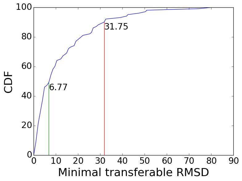
(a) Fast Gradient

(b) Fast Gradient Sign

Figure 1: The CDF of the minimal transferable RMSD from VGG-16 to ResNet-152 using FG (a) and FGS (b). The green line labels the median minimal transferable RMSD, while the red line labels the minimal transferable RMSD to reach 90% percentage.

Figure 1 plots the cumulative distribution function (CDF) of the minimal transferable RMSD from VGG-16 to ResNet-152 using non-targeted FG (Figure 1(a)) and FGS (Figure 1(b)). From the figures, we observe that both FG and FGS can find 100% transferable adversarial images with RMSD less than $80.91$ and $86.56$ respectively. Further, the FG method can generate transferable attacks with smaller RMSD than FGS. A potential reason is that while FGS minimizes the distortion’s $L_{\infty}$ norm, FG minimizes its $L_{2}$ norm, which is proportional to RMSD.

3.3 Comparison with random perturbations

We also evaluate the test accuracy when we add a Gaussian noise to the 100 images in our test set. The concrete results can be found in the appendix, and we show the conclusion that the “transferability” of this approach is significantly worse than either optimization-based approaches or fast gradient-based approaches.

4 Targeted Adversarial Examples

In this section, we examine the transferability of targeted adversarial images. Table 2 presents the results for using optimization-based approach. We observe that (1) the prediction of targeted adversarial images can match the target labels when evaluated on the same model that is used to generate the adversarial examples; but (2) the targeted adversarial images can be rarely predicted as the target labels by a different model. We call the latter that the target labels do not transfer. Even when we increase the distortion, we still do not observe improvements on making target label transfer. Some results can be found in the appendix (Table 17). Even if we compute the matching rate based on top-5 accuracy, the highest matching rate is only 10%. The results can be found in the appendix (Table 18).

	RMSD	ResNet-152	ResNet-101	ResNet-50	VGG-16	GoogLeNet
ResNet-152	23.13	100%	2%	1%	1%	1%
ResNet-101	23.16	3%	100%	3%	2%	1%
ResNet-50	23.06	4%	2%	100%	1%	1%
VGG-16	23.59	2%	1%	2%	100%	1%
GoogLeNet	22.87	1%	1%	0%	1%	100%

Table 2: The matching rate of targeted adversarial images generated using the optimization-based approach. The first column indicates the average RMSD of the generated adversarial images. Cell $(i,j)$ indicates that matching rate of the targeted adversarial images generated for model $i$ (row) when evaluated on model $j$ (column). The top-5 results can be found in the appendix (Table 12).

We also examine the targeted adversarial images generated by fast gradient-based approaches, and we observe that the target labels do not transfer as well. The results are deferred to the appendix (Table 25). In fact, most targeted adversarial images cannot mislead the model, for which the adversarial images are generated, to predict the target labels, regardless of how large the distortion is used. We attribute it to the fact that the fast gradient-based approaches only search for attacks in a 1-D subspace. In this subspace, the total possible predictions may contain a small subset of all labels, which usually does not contain the target label. In Section 6, we study decision boundaries regarding this issue.

We also evaluate the matching rate of images added with Gaussian noise, as described in Section 3.3. However, we observe that the matching rate of any of the 5 models is $0\%$. Therefore, we conclude that by adding Gaussian noise, the attacker cannot generate successful targeted adversarial examples at all, let alone targeted transferability.

5 Ensemble-based approaches

We hypothesize that if an adversarial image remains adversarial for multiple models, then it is more likely to transfer to other models as well. We develop techniques to generate adversarial images for multiple models. The basic idea is to generate adversarial images for the ensemble of the models. Formally, given $k$ white-box models with softmax outputs being $J_{1},...,J_{k}$, an original image $x$, and its ground truth $y$, the ensemble-based approach solves the following optimization problem (for targeted attack):

$$\mathbf{argmin}_{x\star}-\log{\big{(}(\sum_{i=1}^{k}\alpha_{i}J_{i}(x^{\star}))\cdot\mathbf{1}_{y^{\star}}\big{)}}+\lambda d(x,x^{\star})$$ (6)

where $y^{\star}$ is the target label specified by the adversary, $\sum\alpha_{i}J_{i}(x^{\star})$ is the ensemble model, and $\alpha_{i}$ are the ensemble weights, $\sum_{i=1}^{k}\alpha_{i}=1$. Note that (6) is the targeted objective. The non-targeted counterpart can be derived similarly. In doing so, we hope the generated adversarial images remain adversarial for an additional black-box model $J_{k+1}$.

We evaluate the effectiveness of the ensemble-based approach. For each of the five models, we treat it as the black-box model to attack, and generate adversarial images for the ensemble of the rest four, which is considered as white-box. We evaluate the generated adversarial images over all five models. Throughout the rest of the paper, we refer to the approaches evaluated in Section 3 and 4 as the approaches using a single model, and to the ensemble-based approaches discussed in this section as the approaches using an ensemble model.

Optimization-based approach.

We use Adam to optimize the objective (6) with equal ensemble weights across all models in the ensemble to generate targeted adversarial examples. In particular, we set the learning rate of Adam to be $8$ for each model. In each iteration, we compute the Adam update for each model, sum up the four updates, and add the aggregation onto the image. We run 100 iterations of updates, and we observe that the loss converges after 100 iterations. By doing so, for the first time, we observe a large proportion of the targeted adversarial images whose target labels can transfer. The results are presented in Table 3. We observe that not all targeted adversarial images can be misclassified to the target labels by the models used in the ensemble. This suggests that while searching for an adversarial example for the ensemble model, there is no direct supervision to mislead any individual model in the ensemble to predict the target label. Further, from the diagonal numbers of the table, we observe that the transferability to ResNet models is better than to VGG-16 or GoogLeNet, when adversarial examples are generated against all models except the target model.

	RMSD	ResNet-152	ResNet-101	ResNet-50	VGG-16	GoogLeNet
-ResNet-152	30.68	38%	76%	70%	97%	76%
-ResNet-101	30.76	75%	43%	69%	98%	73%
-ResNet-50	30.26	84%	81%	46%	99%	77%
-VGG-16	31.13	74%	78%	68%	24%	63%
-GoogLeNet	29.70	90%	87%	83%	99%	11%

Table 3: The matching rate of targeted adversarial images generated using the optimization-based approach. The first column indicates the average RMSD of the generated adversarial images. Cell $(i,j)$ indicates that percentage of the targeted adversarial images generated for the ensemble of the four models except model $i$ (row) is predicted as the target label by model $j$ (column). In each row, the minus sign “$-$” indicates that the model of the row is not used when generating the attacks. Results of top-5 matching rate can be found in the appendix (Table 13).

We also evaluate non-targeted adversarial images generated by the ensemble-based approach. We observe that the generated adversarial images have almost perfect transferability. We use the same procedure as for the targeted version, except the objective to generate the adversarial images. We evaluate the generated adversarial images over all models. The results are presented in Table 4. The generated adversarial images all have RMSDs around 17, which are lower than 22 to 23 of the optimization-based approach using a single model (See Table 1 for comparison). When the adversarial images are evaluated over models which are not used to generate the attack, the accuracy is no greater than $6\%$. For a reference, the corresponding accuracies for all approaches evaluated in Section 3 using one single model are at least 12%. Our experiments demonstrate that the ensemble-based approaches can generate almost perfectly transferable adversarial images.

	RMSD	ResNet-152	ResNet-101	ResNet-50	VGG-16	GoogLeNet
-ResNet-152	17.17	0%	0%	0%	0%	0%
-ResNet-101	17.25	0%	1%	0%	0%	0%
-ResNet-50	17.25	0%	0%	2%	0%	0%
-VGG-16	17.80	0%	0%	0%	6%	0%
-GoogLeNet	17.41	0%	0%	0%	0%	5%

Table 4: Accuracy of non-targeted adversarial images generated using the optimization-based approach. The first column indicates the average RMSD of the generated adversarial images. Cell $(i,j)$ corresponds to the accuracy of the attack generated using four models except model $i$ (row) when evaluated over model $j$ (column). In each row, the minus sign “$-$” indicates that the model of the row is not used when generating the attacks. Results of top-5 accuracy can be found in the appendix (Table 14).

Fast gradient-based approach.

The results for non-targeted fast gradient-based approaches applied to the ensemble can be found in the appendix (Table 21, 22, 23 and 24). We observe that the diagonal values are not zero, which is the same as we observed in the results for FG and FGS applied to a single model. We hypothesize a potential reason is that the gradient directions of different models in the ensemble are orthogonal to each other, as we will illustrate in Section 6. In this case, the gradient direction of the ensemble is almost orthogonal to the one of each model in the ensemble. Therefore searching along this direction may require large distortion to reach adversarial examples.

For targeted adversarial examples generated using FG and FGS based on an ensemble model, their transferability is no better than the ones generated using a single model. The results can be found in the appendix (Table 28, 29, 30 and 31). We hypothesize the same reason to explain this: there are only few possible target labels in total in the 1-D subspace.

6 Geometric Properties of Different Models

In this section, we show some geometric properties of the models to try to better understand transferable adversarial examples. Prior works also try to understand the geometic properties of adversarial examples theoretically (Fawzi et al. (2016)) or empirically (Goodfellow et al. (2014)). In this work, we examine large models trained over a large dataset with 1000 labels, whose geometric properties are never examined before. This allows us to make new observations to better understand the models and their adversarial examples.

The gradient directions of different models in our evaluation are almost orthogonal to each other.

We study whether the adversarial directions of different models align with each other. We calculate cosine value of the angle between gradient directions of different models, and the results can be found in the appendix (Table 33). We observe that all non-diagonal values are close to 0, which indicates that for most images, their gradient directions with respect to different models are orthogonal to each other.

Figure 2: The example image to study the decision boundary. Its ID in ILSVRC 2012 validation set is 49443, and its ground truth label is “anemone fish.”

	VGG-16	ResNet-50	ResNet-101	ResNet-152	GoogLeNet
Zoom-in
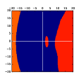
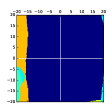
Zoom-out

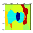
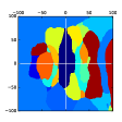
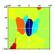
Figure 3: Decision regions of different models. We pick the same two directions for all plots: one is the gradient direction of VGG-16 (x-axis), and the other is a random orthogonal direction (y-axis). Each point in the span plane shows the predicted label of the image generated by adding a noise to the original image (e.g., the origin corresponds to the predicted label of the original image). The units of both axises are 1 pixel values. All sub-figure plots the regions on the span plane using the same color for the same label. The image is in Figure 2.

Model	VGG-16	ResNet-50	ResNet-101	ResNet-152	GoogLeNet
# of labels	10	9	21	10	21

Table 5: The number of all possible predicted labels for each model in the same plane described in Figure 3.

Decision boundaries of the non-targeted approaches using a single model.

We study the decision boundary of different models to understand why adversarial examples transfer. We choose two normalized orthogonal directions $\delta_{1},\delta_{2}$, one being the gradient direction of VGG-16 and the other being randomly chosen. Each point $(u,v)$ in this 2-D plane corresponds to the image $x+u\delta_{1}+v\delta_{2}$, where $x$ is the pixel value vector of the original image. For each model, we plot the label of the image corresponding to each point, and get Figure 3 using the image in Figure 2.

We can observe that for all models, the region that each model can predict the image correctly is limited to the central area. Also, along the gradient direction, the classifiers are soon misled. One interesting finding is that along this gradient direction, the first misclassified label for the three ResNet models (corresponding to the light green region) is the label “orange”. A more detailed study can be found in the appendix (Table 9, Table 26 and 27). When we look at the zoom-out figures, however, the labels of images that are far away from the original one are different for different models, even among ResNet models.

On the other hand, in Table 5, we show the total number of regions in each plane. In fact, for each plane, there are at most 21 different regions in all planes. Compared with the 1,000 total categories in ImageNet, this is only 2.1% of all categories. That means, for all other 97.9% labels, no targeted adversarial example exists in each plane. Such a phenomenon partially explains why fast gradient-based approaches can hardly find targeted adversarial images.

Figure 4: The decision boundary to separate the region within which all points are classified as the ground truth label (encircled by each closed curve) from others. The plane is the same one described in Figure 3. The origin of the coordinate plane corresponds to the original image. The units of both axises are 1 pixel values.

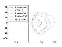
Figure 5: The decision boundary to separate the region within which all points are classified as the target label (encircled by each closed curve) from others. The plane is spanned by the targeted adversarial direction and a random orthogonal direction. The targeted adversarial direction is computed as the difference between the original image in Figure 2 and the adversarial image generated by the optimization-based approach for an ensemble. The ensemble contains all models except ResNet-101. The origin of the coordinate plane corresponds to the original image. The units of both axises are 1 pixel values.

Further, in Figure 5, we draw the decision boundaries of all models on the same plane as described above. We can observe that

• The boundaries align with each other very well. This partially explains why non-targeted adversarial images can transfer among models.

• The boundary diameters along the gradient direction is less than the ones along the random direction. A potential reason is that moving a variable along its gradient direction can change the loss function (i.e., the probability of the ground truth label) significantly. Therefore along the gradient direction it will take fewer steps to move out of the ground truth region than a random direction.

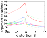
(a) GoogLeNet

(b) VGG-16

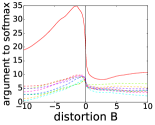
(c) ResNet-152

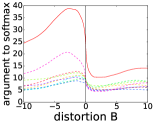
(d) ResNet-101

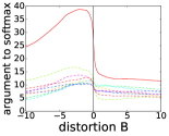
(e) ResNet-50

Figure 7: Linearity of different models. Each line plots the classification layer’s softmax input vs distortion $B$ when fast gradient noises are used. Solid red line is the ground truth label, and other lines are the top 10 labels predicted on the original image.

• An interesting finding is that even though we move left along the x-axis, which is equivalent to maximizing the ground truth’s prediction probability, it also reaches the boundary much sooner than moving along a random direction. We attribute this to the non-linearity of the loss function: when the distortion is larger, the gradient direction also changes dramatically. In this case, moving along the original gradient direction no longer increases the probability to predict the ground truth label (see Figure 7 in the appendix).

• As for VGG-16 model, there is a small hole within the region corresponding to the ground truth. This may partially explain why non-targeted adversarial images with small distortion exist, but do not transfer well. This hole does not exist in other models’ decision planes. In this case, non-targeted adversarial images in this hole do not transfer.

Decision boundaries of the targeted ensemble-based approaches.

In addition, we choose the targeted adversarial direction of the ensemble of all models except ResNet-101 and a random orthogonal direction, and we plot decision boundaries on the plane spanned by these two direction vectors in Figure 5. We observe that the regions of images, which are predicted as the target label, align well for the four models in the ensemble. However, for the model not used to generate the adversarial image, i.e., ResNet-101, it also has a non-empty region such that the prediction is successfully misled to the target label, although the area is much smaller. Meanwhile, the region within each closed curve of the models almost has the same center.

7 Real world example: adversarial examples for Clarifai.com

Clarifai.com is a commercial company providing state-of-the-art image classification services. We have no knowledge about the dataset and types of models used behind Clarifai.com, except that we have black-box access to the services. The labels returned from Clarifai.com are also different from the categories in ILSVRC 2012. We submit all 100 original images to Clarifai.com and the returned labels are correct based on a subjective measure.

We also submit 400 adversarial images in total, where 200 of them are targeted adversarial examples, and the rest 200 are non-targeted ones. As for the 200 targeted adversarial images, 100 of them are generated using the optimization-based approach based on VGG-16 (the same ones evaluated in Table 2), and the rest 100 are generated using the optimization-based approach based on an ensemble of all models except ResNet-152 (the same ones evaluated in Table 3). The 200 non-targeted adversarial examples are generated similarly (the same ones evaluated in Table 1 and 4).

For non-targeted adversarial examples, we observe that for both the ones generated using VGG-16 and those generated using the ensemble, most of them can transfer to Clarifai.com.

More importantly, a large proportion of our targeted adversarial examples are misclassified by Clarifai.com as well. We observe that $57\%$ of the targeted adversarial examples generated using VGG-16, and $76\%$ of the ones generated using the ensemble can mislead Clarifai.com to predict labels irrelevant to the ground truth.

Further, our experiment shows that for targeted adversarial examples, $18\%$ of those generated using the ensemble model can be predicted as labels close to the target label by Clarifai.com. The corresponding number for the targeted adversarial examples generated using VGG-16 is $2\%$. Considering that in the case of attacking Clarifai.com, the labels given by the target model are different from those given by our models, it is fairly surprising to see that when using the ensemble-based approach, there is still a considerable proportion of our targeted adversarial examples that can mislead this black-box model to make predictions semantically similar to our target labels. All these numbers are computed based on a subjective measure, and we include some examples in Table LABEL:tab:real-exmp. More examples can be found in the appendix (Table LABEL:tab:real-app).

Table 6: Original images and adversarial images evaluated over Clarifai.com. For labels returned from Clarifai.com, we sort the labels firstly by rareness: how many times a label appears in the Clarifai.com results for all adversarial images and original images, and secondly by confidence. Only top 5 labels are provided.

original image	true label	Clarifai.com results of original image	target label	targeted adversarial example	Clarifai.com results of targeted adversarial example
	viaduct	bridge,
sight,
arch,
river,
sky	window screen		window,
wall,
old,
decoration,
design
	hip, rose hip, rosehip	fruit,
fall,
food,
little,
wildlife	stupa, tope		Buddha,
gold,
temple,
celebration,
artistic
	dogsled, dog sled, dog sleigh	group together,
four,
sledge,
sled,
enjoyment	hip, rose hip, rosehip		cherry,
branch,
fruit,
food,
season
	pug, pug-dog	pug,
friendship,
adorable,
purebred,
sit	sea lion		sea seal,
ocean,
head,
sea,
cute
	Old English sheepdog, bobtail	poodle,
retriever,
loyalty,
sit,
two	abaya		veil,
spirituality,
religion,
people,
illustration
	maillot, tank suit	beach,
woman,
adult,
wear,
portrait	amphibian, amphibious vehicle		transportation system,
vehicle,
man,
print,
retro
	patas, hussar monkey, Erythrocebus patas	primate,
monkey,
safari,
sit,
looking	bee eater		ornithology,
avian,
beak,
wing,
feather

8 Conclusion

In this work, we are the first to conduct an extensive study of the transferability of both non-targeted and targeted adversarial examples generated using different approaches over large models and a large scale dataset. Our results confirm that the transferability for non-targeted adversarial examples are prominent even for large models and a large scale dataset. On the other hand, we find that it is hard to use existing approaches to generate targeted adversarial examples whose target labels can transfer. We develop novel ensemble-based approaches, and demonstrate that they can generate transferable targeted adversarial examples with a high success rate. Meanwhile, these new approaches exhibit better performance on generating non-targeted transferable adversarial examples than previous work. We also show that both non-targeted and targeted adversarial examples generated using our new approaches can successfully attack Clarifai.com, which is a black-box image classification system. Furthermore, we study some geometric properties to better understand the transferable adversarial examples.

Acknowledgments

This material is in part based upon work supported by the National Science Foundation under Grant No. TWC-1409915. Any opinions, findings, and conclusions or recommendations expressed in this material are those of the author(s) and do not necessarily reflect the views of the National Science Foundation.

Appendix

	ResNet-50	ResNet-101	ResNet-152	GoogLeNet	VGG-16
Top-1 accuracy	72.5%	73.8%	74.6%	68.7%	68.3%
Top-5 accuracy	91.0%	91.7%	92.1%	89.0%	88.3%

Table 7: Top-1 and top-5 accuracy of the studied models over the ILSVRC 2012 validation dataset.

	RMSD	ResNet-152	ResNet-101	ResNet-50	VGG-16	GoogLeNet
ResNet-152	22.83	7%	43%	43%	39%	31%
ResNet-101	23.81	40%	6%	41%	42%	34%
ResNet-50	22.86	48%	44%	3%	42%	32%
VGG-16	22.51	36%	33%	33%	0%	15%
GoogLeNet	22.58	66%	71%	62%	49%	2%

Table 8: Top-5 accuracy of Table 1 Panel A. Transferability between pairs of models using non-targeted optimization-based approach with a learning rate of 4. The first column indicates the average RMSD of all adversarial images generated for the model in the corresponding row. The cell $(i,j)$ indicates the top-5 accuracy of the adversarial images generated for model $i$ (row) evaluated over model $j$ (column). Lower value indicates better transferability.

An alternative optimization-based approach to generate adversarial examples.

An alternative method to generate non-targeted adversarial examples with large distortion is to revise the optimization objective to incorporate this distortion constraint. For example, for non-targeted adversarial image searching, we can optimize for the following objective.

$$\mathbf{argmin}_{x^{\star}}-\log{(1-\mathbf{1}_{y}\cdot J_{\theta}(x^{\star}))}+\lambda_{1}\mathrm{ReLU}(\tau-d(x,x^{\star}))+\lambda_{2}\mathrm{ReLU}(d(x,x^{\star})-\tau)$$

Optimizing for the above objective has the following three effects: (1) minimizing $-\log{(1-\mathbf{1}_{y}\cdot J_{\theta}(x^{\star}))}$; (2) Penalizing the solution if $d(x,x^{\star})$ is no more than a threshold $\tau$ (too low); and (3) Penalizing the solution if $d(x,x^{\star})$ is too high.

In our preliminary evaluation, we found that the solutions computed from the two approaches have similar transferability. We thus omit the results for this alternative approach.

Transferable non-targeted adversarial images are classified as the same wrong labels.

Previous work Goodfellow et al. (2014) reported the phenomenon that when evaluating the adversarial images, different models tend to make the same wrong predictions. This conclusion was only examined over datasets with 10 categories. In our evaluation, however, we observe the same phenomenon, albeit we have 1000 possible categories. We refer to this effect as the same mistake effect.

Table 9 presents the results based on the adversarial examples generated for VGG-16. For each pair of models, among all adversarial examples that both models make wrong predictions, we compute the percentage that both models make the same mistake. These percentage numbers are from 12% to 40%, which are surprisingly high, since there are 999 possible categories to be misclassified into (see Table 32 in the appendix for the wrong predicted label distribution of these adversarial examples). Later in Section 6, we try to explain this phenomenon using decision boundaries.

ResNet-152 ResNet-101 ResNet-50 VGG-16 GoogLeNet ResNet-152 100.00% $-$ $-$ $-$ $-$ ResNet-101 28.57% 100.00% $-$ $-$ $-$ ResNet-50 29.87% 40.00% 100.00% $-$ $-$ VGG-16 19.23% 18.07% 22.89% 100.00% $-$ GoogLeNet 12.82% 20.48% 18.07% 16.84% 100.00%

Table 9: When using the optimization-based approach for VGG-16 model to generate non-targeted adversarial images, cell $(i,j)$ is the percentage of all transferable adversarial images that are predicted as the same wrong labels by both models $i$ and $j$ over all adversarial images that are misclassified by both models $i$ and $j$. Notice that this table is symmetric.

Adversarial images may come from multiple intervals along the gradient direction.

In Figure 6, we show that along the gradient direction of the non-targeted objective (3) for VGG-16, when evaluating the adversarial image $x_{B}$ on ResNet-152, $x_{B}$ will soon become adversarial for small $B$. While $B$ increases, however, the prediction changes back to be the correct label, then a wrong label, then the correct label again, and finally wrong labels. This indicates that along the gradient of this image, the distortions that can cause the corresponding adversarial images to mislead ResNet-152 form four intervals.

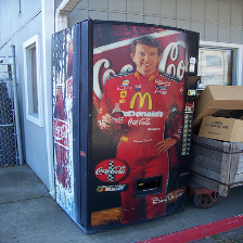
(a) The original image

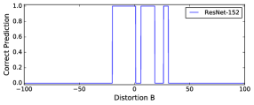
(b) Prediction correctness

Figure 6: We add $B\delta$ onto the original image in Figure 6(a), where $\delta$ is the normalized gradient of the non-targeted objective (3) for VGG-16. When $x_{B}$ is evaluated on ResNet-152, we plot 1 if the prediction matches the ground truth, or 0 otherwise.

	RMSD	ResNet-152	ResNet-101	ResNet-50	VGG-16	GoogLeNet
ResNet-152	23.45	23%	29%	31%	39%	33%
ResNet-101	23.49	35%	20%	33%	43%	28%
ResNet-50	23.49	40%	39%	18%	39%	33%
VGG-16	23.73	40%	35%	33%	8%	19%
GoogLeNet	23.45	53%	46%	37%	38%	7%

Table 10: Top-5 accuracy of Table 1 Panel B. Transferability between pairs of models using non-targeted FG. The first column indicates the average RMSD of all adversarial images generated for the model in the corresponding row. The cell $(i,j)$ indicates the top-5 accuracy of the adversarial images generated for model $i$ (row) evaluated over model $j$ (column). Lower value indicates better transferability.

Comparison with random perturbations.

For comparison, we evaluate the test accuracy when we add a Gaussian noise to the 100 images in our test set. We vary the standard deviation of the Gaussian noise from 5 to 40 with a step size of 5. For each specific standard deviation, we generate 100 random noises and add them to each image, resulting in 10,000 noisy images in total. Then we evaluate the accuracy of each model on these 10,000 images, and the results are presented in Table 11. Notice that when setting standard deviation to be $25$, the average RMSD is 23.59, which is comparable to that of non-targeted adversarial examples generated by either optimization-based approaches or fast gradient-based approaches. However, each model can still achieve an accuracy more than $66\%$. This shows that adding random noise is not an effective way to generate adversarial examples, hence the “transferability” of this approach is significantly worse than either optimization-based approaches or fast gradient-based approaches.

Standard Deviation	RMSD	ResNet-152	ResNet-101	ResNet-50	VGG-16	GoogLeNet
5	4.91	97.41%	98.96%	98.74%	97.47%	99.29%
10	9.72	95.53%	96.72%	96.81%	92.13%	95.94%
15	14.44	91.19%	94.22%	92.16%	87.86%	88.50%
20	19.07	86.56%	90.38%	84.07%	82.30%	77.84%
25	23.59	83.10%	85.53%	78.33%	73.57%	66.84%
30	28.01	78.95%	79.04%	71.66%	65.33%	54.93%
35	32.32	73.60%	70.89%	62.03%	58.55%	45.13%
40	36.52	66.53%	63.09%	50.96%	51.85%	35.61%

Table 11: Accuracy of images with random perturbation. The first column reports the standard deviation of the Gaussian noise added to each image. The second column reports the average RMSD over all generated images with the respective standard deviation. For each of the rest column $j$, the cell $(i,j)$ reports model $j$’s accuracy of the noisy images when a Gaussian noise with the respective standard deviation specified in row $i$ is added to each image.

	RMSD	ResNet-152	ResNet-101	ResNet-50	VGG-16	GoogLeNet
ResNet-152	23.13	100%	11%	5%	3%	1%
ResNet-101	23.16	9%	100%	7%	2%	1%
ResNet-50	23.06	10%	9%	100%	2%	3%
VGG-16	23.59	3%	5%	5%	100%	4%
GoogLeNet	22.87	1%	2%	1%	3%	100%

Table 12: Top-5 matching rate of Table 2. The adversarial images are generated using the targeted optimization-based approach with a learning rate of 4. The first column indicates the average RMSD of all adversarial images generated for the model in the corresponding row. Cell $(i,j)$ indicates that top-5 matching rate of the targeted adversarial images generated for model $i$ (row) when evaluated on model $j$ (column). Higher value indicates more successful transferable target labels.

	RMSD	ResNet-152	ResNet-101	ResNet-50	VGG-16	GoogLeNet
-ResNet-152	30.68	87%	100%	100%	100%	100%
-ResNet-101	30.76	100%	88%	100%	100%	100%
-ResNet-50	30.26	99%	99%	86%	99%	99%
-VGG-16	31.13	100%	100%	100%	51%	100%
-GoogLeNet	29.70	100%	100%	100%	100%	32%

Table 13: The top-5 matching rate of Table 3. Matching rate of adversarial images generated using targeted optimization-based approach. The first column indicates the average RMSD of all adversarial images generated for the model in the corresponding row. Cell $(i,j)$ indicates that top-5 matching rate of the targeted adversarial images generated using the ensemble of the four models except model $i$ (row) is predicted as the target label by model $j$ (column). In each row, the minus sign “$-$” indicates that the model of the row is not used when generating the attacks. Higher value indicates more successful transferable target labels.

	RMSD	ResNet-152	ResNet-101	ResNet-50	VGG-16	GoogLeNet
-ResNet-152	17.17	13%	4%	4%	0%	3%
-ResNet-101	17.25	2%	11%	3%	0%	3%
-ResNet-50	17.25	4%	5%	11%	0%	2%
-VGG-16	17.80	4%	7%	5%	20%	4%
-GoogLeNet	17.41	3%	2%	3%	0%	15%

Table 14: Top-5 accuracy of Table 4. The first column indicates the average RMSD of all adversarial images generated for the model in the corresponding row. Cell $(i,j)$ indicates that top-5 accuracy of the non-targeted adversarial images generated using the ensemble of the four models except model $i$ (row) when evaluated over model $j$ (column). In each row, the minus sign “$-$” indicates that the model of the row is not used when generating the attacks. Lower value indicates better transferability.

	RMSD	ResNet-152	ResNet-101	ResNet-50	VGG-16	GoogLeNet
ResNet-152	1.25	0%	86%	87%	93%	96%
ResNet-101	1.24	84%	0%	93%	95%	100%
ResNet-50	1.21	90%	91%	0%	91%	97%
VGG-16	1.55	89%	94%	92%	0%	84%
GoogLeNet	1.27	94%	97%	98%	91%	0%

Table 15: Transferability between pairs of models using non-targeted optimization-based approach with a learning rate of 0.125. The first column indicates the average RMSD of all adversarial images generated for the model in the corresponding row. The cell $(i,j)$ indicates the top-1 accuracy of the adversarial images generated for model $i$ (row) evaluated over model $j$ (column). Lower value indicates better transferability. Results of top-5 accuracy can be found in Table 16.

	RMSD	ResNet-152	ResNet-101	ResNet-50	VGG-16	GoogLeNet
ResNet-152	1.25	24%	100%	100%	99%	100%
ResNet-101	1.24	100%	22%	99%	100%	100%
ResNet-50	1.21	100%	99%	25%	100%	100%
VGG-16	1.55	98%	100%	100%	15%	100%
GoogLeNet	1.27	100%	100%	100%	100%	18%

Table 16: Top-5 accuracy of Table 15. Transferability between pairs of models using non-targeted optimization-based approach with a learning rate of 0.125. The first column indicates the average RMSD of all adversarial images generated for the model in the corresponding row. The cell $(i,j)$ indicates the top-5 accuracy of the adversarial images generated for model $i$ (row) evaluated over model $j$ (column). Lower value indicates better transferability.

	RMSD	ResNet-152	ResNet-101	ResNet-50	VGG-16	GoogLeNet
ResNet-152	31.35	98%	1%	2%	2%	0%
ResNet-101	31.11	5%	98%	1%	2%	0%
ResNet-50	31.32	3%	2%	99%	1%	1%
VGG-16	31.50	1%	1%	2%	97%	1%
GoogLeNet	30.67	2%	1%	0%	2%	97%

Table 17: The adversarial images are generated using the targeted optimization-based approach with a larger learning rate. The first column indicates the average RMSD of all adversarial images generated for the model in the corresponding row. Cell $(i,j)$ indicates that top-1 matching rate of the targeted adversarial images generated for model $i$ (row) when evaluated on model $j$ (column). Higher value indicates more successful transferable target labels. We used a larger learning rate to achieve larger RMSD. Results of top-5 matching rate can be found in Table 18.

	RMSD	ResNet-152	ResNet-101	ResNet-50	VGG-16	GoogLeNet
ResNet-152	31.35	98%	8%	6%	3%	1%
ResNet-101	31.11	10%	98%	5%	3%	1%
ResNet-50	31.32	6%	7%	99%	5%	1%
VGG-16	31.50	4%	4%	6%	97%	4%
GoogLeNet	30.67	3%	1%	2%	3%	97%

Table 18: The top-5 matching rate of Table 17. The adversarial images are generated using the targeted optimization-based approach with a larger learning rate. The first column indicates the average RMSD of all adversarial images generated for the model in the corresponding row. Cell $(i,j)$ indicates that top-5 matching rate of the targeted adversarial images generated for model $i$ (row) when evaluated on model $j$ (column). Higher value indicates more successful transferable target labels. We used a larger learning rate to achieve larger RMSD.

	RMSD	ResNet-152	ResNet-101	ResNet-50	VGG-16	GoogLeNet
ResNet-152	23.11	12%	27%	25%	22%	15%
ResNet-101	23.11	29%	13%	29%	29%	16%
ResNet-50	23.11	34%	28%	10%	25%	23%
VGG-16	23.12	25%	20%	23%	0%	8%
GoogLeNet	23.11	46%	41%	40%	25%	2%

Table 19: Transferability between pairs of models using non-targeted FGS. The first column indicates the average RMSD of all adversarial images generated for the model in the corresponding row. The cell $(i,j)$ indicates the top-1 accuracy of the adversarial images generated for model $i$ (row) evaluated over model $j$ (column). Lower value indicates better transferability. Results of top-5 accuracy can be found in Table 20.

	RMSD	ResNet-152	ResNet-101	ResNet-50	VGG-16	GoogLeNet
ResNet-152	23.11	32%	55%	53%	47%	36%
ResNet-101	23.11	56%	33%	50%	46%	40%
ResNet-50	23.11	59%	53%	29%	47%	38%
VGG-16	23.12	42%	39%	41%	5%	21%
GoogLeNet	23.11	71%	74%	62%	53%	11%

Table 20: Top-5 accuracy of Table 19. Transferability between pairs of models using non-targeted FGS. The first column indicates the average RMSD of all adversarial images generated for the model in the corresponding row. The cell $(i,j)$ indicates the top-5 accuracy of the adversarial images generated for model $i$ (row) evaluated over model $j$ (column). Lower value indicates better transferability.

	RMSD	ResNet-152	ResNet-101	ResNet-50	VGG-16	GoogLeNet
-ResNet-152	17.25	23%	12%	11%	1%	7%
-ResNet-101	17.24	15%	19%	11%	2%	6%
-ResNet-50	17.24	15%	13%	19%	2%	8%
-VGG-16	17.24	17%	15%	12%	23%	7%
-GoogLeNet	17.24	14%	11%	10%	2%	19%

Table 21: Transferability between pairs of models using non-targeted ensemble FG. The first column indicates the average RMSD of the generated adversarial images. Cell $(i,j)$ indicates that top-1 accuracy of the non-targeted adversarial images generated using the ensemble of the four models except model $i$ (row) when evaluated over model $j$ (column). In each row, the minus sign “$-$” indicates that the model of the row is not used when generating the attacks. Lower value indicates better transferability. Results of top-5 accuracy can be found in Table 22.

	RMSD	ResNet-152	ResNet-101	ResNet-50	VGG-16	GoogLeNet
-ResNet-152	17.25	47%	33%	28%	15%	21%
-ResNet-101	17.24	37%	42%	30%	14%	26%
-ResNet-50	17.24	38%	32%	39%	13%	23%
-VGG-16	17.24	37%	36%	37%	44%	32%
-GoogLeNet	17.24	32%	30%	28%	13%	46%

Table 22: Top-5 accuracy of Table 21. Transferability between pairs of models using non-targeted ensemble FG. The first column indicates the average RMSD of the generated adversarial images. Cell $(i,j)$ indicates that top-5 accuracy of the non-targeted adversarial images generated using the ensemble of the four models except model $i$ (row) when evaluated over model $j$ (column). In each row, the minus sign “$-$” indicates that the model of the row is not used when generating the attacks. Lower value indicates better transferability.

	RMSD	ResNet-152	ResNet-101	ResNet-50	VGG-16	GoogLeNet
-ResNet-152	17.41	26%	10%	11%	2%	7%
-ResNet-101	17.40	18%	21%	13%	2%	4%
-ResNet-50	17.40	15%	13%	20%	4%	8%
-VGG-16	17.40	17%	16%	11%	23%	7%
-GoogLeNet	17.40	15%	12%	10%	3%	22%

Table 23: Transferability between pairs of models using non-targeted ensemble FGS. The first column indicates the average RMSD of the generated adversarial images. Cell $(i,j)$ indicates that top-1 accuracy of the non-targeted adversarial images generated using the ensemble of the four models except model $i$ (row) when evaluated over model $j$ (column). In each row, the minus sign “$-$” indicates that the model of the row is not used when generating the attacks. Lower value indicates better transferability. Results of top-5 accuracy can be found in Table 24.

	RMSD	ResNet-152	ResNet-101	ResNet-50	VGG-16	GoogLeNet
-ResNet-152	17.41	50%	35%	30%	20%	26%
-ResNet-101	17.40	38%	48%	33%	19%	26%
-ResNet-50	17.40	38%	36%	41%	18%	28%
-VGG-16	17.40	37%	36%	36%	48%	33%
-GoogLeNet	17.40	35%	29%	31%	19%	53%

Table 24: Top-5 accuracy of Table 23. Transferability between pairs of models using non-targeted ensemble FGS. The first column indicates the average RMSD of the generated adversarial images. Cell $(i,j)$ indicates that top-5 accuracy of the non-targeted adversarial images generated using the ensemble of the four models except model $i$ (row) when evaluated over model $j$ (column). In each row, the minus sign “$-$” indicates that the model of the row is not used when generating the attacks. Lower value indicates better transferability.

	RMSD	ResNet-152	ResNet-101	ResNet-50	VGG-16	GoogLeNet
ResNet-152	23.55	1%	2%	0%	0%	1%
ResNet-101	23.56	1%	1%	0%	0%	1%
ResNet-50	23.56	1%	1%	1%	0%	0%
VGG-16	23.95	1%	1%	0%	1%	1%
GoogLeNet	23.63	1%	1%	0%	1%	1%

Table 25: The adversarial images are generated using the targeted FG. The first column indicates the average RMSD of all adversarial images generated for the model in the corresponding row. The first column indicates the average RMSD of the generated adversarial images. Cell $(i,j)$ indicates that top-1 matching rate of the targeted adversarial images generated for model $i$ (row) when evaluated on model $j$ (column). Higher value indicates more successful transferable target labels.

	ResNet-152	ResNet-101	ResNet-50	VGG-16	GoogLeNet
ResNet-152	100.00%	$-$	$-$	$-$	$-$
ResNet-101	33.33%	100.00%	$-$	$-$	$-$
ResNet-50	24.00%	35.00%	100.00%	$-$	$-$
VGG-16	17.50%	19.05%	21.18%	100.00%	$-$
GoogLeNet	15.38%	14.81%	13.10%	15.05%	100.00%

Table 26: When using non-targeted FG for VGG-16 model to generate adversarial images, cell $(i,j)$ is the percentage of all transferable adversarial images that are predicted as the same wrong labels by both models $i$ and $j$ over all adversarial images that are misclassified by both models $i$ and $j$. Notice that the table is symmetric.

	ResNet-152	ResNet-101	ResNet-50	VGG-16	GoogLeNet
ResNet-152	100.00%	$-$	$-$	$-$	$-$
ResNet-101	33.78%	100.00%	$-$	$-$	$-$
ResNet-50	36.62%	43.24%	100.00%	$-$	$-$
VGG-16	16.00%	20.00%	23.38%	100.00%	$-$
GoogLeNet	14.86%	20.25%	13.16%	19.57%	100.00%

Table 27: When using non-targeted FGS for VGG-16 model to generate adversarial images, cell $(i,j)$ is the percentage of all transferable adversarial images that are predicted as the same wrong labels by both models $i$ and $j$ over all adversarial images that are misclassified by both models $i$ and $j$. Notice that the table is symmetric.

	RMSD	ResNet-152	ResNet-101	ResNet-50	VGG-16	GoogLeNet
-ResNet-152	31.05	1%	1%	0%	1%	1%
-ResNet-101	30.94	1%	1%	0%	1%	0%
-ResNet-50	31.12	1%	1%	0%	1%	1%
-VGG-16	30.57	1%	1%	0%	1%	1%
-GoogLeNet	30.47	1%	1%	0%	1%	0%

Table 28: Transferability between pairs of models using targeted ensemble FG. The first column indicates the average RMSD of all adversarial images generated for the model in the corresponding row. Cell $(i,j)$ indicates that top-1 matching rate of the targeted adversarial images generated using the ensemble of the four models except model $i$ (row) is predicted as the target label by model $j$ (column). In each row, the minus sign “$-$” indicates that the model of the row is not used when generating the attacks. Higher value indicates more successful transferable target labels. Results of top-5 matching rate can be found in Table 29.

	RMSD	ResNet-152	ResNet-101	ResNet-50	VGG-16	GoogLeNet
-ResNet-152	31.05	1%	2%	1%	3%	2%
-ResNet-101	30.94	1%	1%	1%	1%	2%
-ResNet-50	31.12	1%	2%	1%	3%	2%
-VGG-16	30.57	2%	2%	2%	1%	1%
-GoogLeNet	30.47	1%	1%	1%	2%	2%

Table 29: Top-5 matching rate of Table 28. Transferability between pairs of models using targeted ensemble FG. The first column indicates the average RMSD of all adversarial images generated for the model in the corresponding row. Cell $(i,j)$ indicates that top-5 matching rate of the targeted adversarial images generated using the ensemble of the four models except model $i$ (row) is predicted as the target label by model $j$ (column). In each row, the minus sign “$-$” indicates that the model of the row is not used when generating the attacks. Higher value indicates more successful transferable target labels.

	RMSD	ResNet-152	ResNet-101	ResNet-50	VGG-16	GoogLeNet
-ResNet-152	30.42	1%	1%	1%	1%	1%
-ResNet-101	30.42	1%	1%	1%	1%	1%
-ResNet-50	30.42	1%	1%	0%	1%	1%
-VGG-16	30.41	1%	1%	0%	1%	1%
-GoogLeNet	30.42	1%	1%	1%	1%	1%

Table 30: Transferability between pairs of models using targeted ensemble FGS. The first column indicates the average RMSD of all adversarial images generated for the model in the corresponding row. Cell $(i,j)$ indicates that top-1 matching rate of the targeted adversarial images generated using the ensemble of the four models except model $i$ (row) is predicted as the target label by model $j$ (column). In each row, the minus sign “$-$” indicates that the model of the row is not used when generating the attacks. Higher value indicates more successful transferable target labels. Results are top-5 matching rate can be found in Table 31.

	RMSD	ResNet-152	ResNet-101	ResNet-50	VGG-16	GoogLeNet
-ResNet-152	30.42	2%	1%	2%	1%	2%
-ResNet-101	30.42	2%	1%	1%	1%	2%
-ResNet-50	30.42	2%	1%	1%	1%	2%
-VGG-16	30.41	3%	2%	2%	1%	1%
-GoogLeNet	30.42	2%	2%	2%	2%	2%

Table 31: Top-5 matching rate of Table 30. Transferability between pairs of models using targeted ensemble FGS. The first column indicates the average RMSD of all adversarial images generated for the model in the corresponding row. Cell $(i,j)$ indicates that top-5 matching rate of the targeted adversarial images generated using the ensemble of the four models except model $i$ (row) is predicted as the target label by model $j$ (column). In each row, the minus sign “$-$” indicates that the model of the row is not used when generating the attacks. Higher value indicates more successful transferable target labels.

ResNet-152	ResNet-101	ResNet-50	VGG-16	GoogleNet
jigsaw puzzle(8%)	jigsaw puzzle(12%)	jigsaw puzzle(12%)	jigsaw puzzle(15%)	prayer rug(12%)
acorn(3%)	starfish(3%)	African chameleon(2%)	African chameleon(7%)	jigsaw puzzle(7%)
lycaenid(2%)	strawberry(2%)	strawberry(2%)	prayer rug(5%)	stole(6%)
ram(2%)	wild boar(2%)	starfish(2%)	apron(4%)	African chameleon(4%)
maze(2%)	dishrag(2%)	greenhouse(2%)	sarong(3%)	mitten(3%)

Table 32: When using non-targeted optimization-based approach for VGG-16 model to generate adversarial images, column $i$ indicates the top 5 common incorrect labels predicted by model $i$. The value in the parentheses is the percentage of the predicted label.

	ResNet-152	ResNet-101	ResNet-50	VGG-16	GoogLeNet
ResNet-152	1.00	$-$	$-$	$-$	$-$
ResNet-101	0.04	1.00	$-$	$-$	$-$
ResNet-50	0.03	0.03	1.00	$-$	$-$
VGG-16	0.02	0.02	0.02	1.00	$-$
GoogLeNet	0.01	0.01	0.01	0.02	1.00

Table 33: Average cosine value of the angle between gradient directions of two models. Notice that the dot-product of two normalized vectors is the cosine value of the angle between them, for each image, we compute the dot-product of normalized gradient directions with respect to model $i$ (row) and model $j$ (column), and the value in cell $(i,j)$ is the average over dot-product values of all images. Notice that this table is symmetric.

More examples submitted to Clarifai.com.

We present more results from Clarifai.com by submitting original and adversarial examples in Table LABEL:tab:real-app.

Table 34: Original images and adversarial images evaluated over Clarifai.com. For labels returned from Clarifai.com, we sort the labels firstly by the occurrence of a label from the Clarifai.com results, and secondly by confidence. Only top 5 labels are provided.

original image	true label	Clarifai.com results of original image	target label	targeted adv-example	Clarifai.com result of targeted adversarial example
	broom	dust,
brick,
rustic,
stone,
dirty	jacamar		feather,
beautiful,
bird,
leaf,
flora
	junco, snowbird	frost,
sparrow,
pigeon,
ice,
frosty	eel		swimming,
underwater,
fish,
water,
one
	harvester, reaper	heavy,
bulldozer,
exert,
track,
plow	prairie chicken, prairie grouse, prairie fowl		wildlife,
animal,
illustration,
nature,
color
	mongoose	fox,
rodent,
predator,
fur,
park	maillot		motley,
shape,
horizontal,
abstract,
bright
	holster	pistol,
force,
bullet,
protection,
cartridge	ground beetle, carabid beetle		shell,
shell (food),
antenna,
insect,
invertebrate
	yurt	wooden,
scenic,
snow,
rural,
landscape	comic book		graffiti,
religion,
people,
painting,
culture
	broccoli	kind,
cauliflower,
vitamin,
carrot,
cabbage	hamster		bird,
bright,
texture,
animal,
decoration
	water buffalo, water ox, Asiatic buffalo, Bubalus bubalis	herd,
milk,
beef cattle,
farmland,
cow	rugby ball		pastime,
print,
illustration,
art
	zebra	equid,
stripe,
savanna,
zebra,
safari	apiary, bee house		wood,
people,
outdoors,
nature
	French bulldog	bulldog,
studio,
boxer,
eye,
bull	kite		visuals,
feather,
wing,
pet,
print
	curly-coated retriever	eye,
looking,
pet,
canine,
dog	fly		graphic,
shape,
insect,
artistic,
image

References

- Carlini & Wagner (2016) Nicholas Carlini and David Wagner. Towards evaluating the robustness of neural networks. arXiv preprint arXiv:1608.04644, 2016.
- Fawzi et al. (2016) Alhussein Fawzi, Seyed-Mohsen Moosavi-Dezfooli, and Pascal Frossard. Robustness of classifiers: from adversarial to random noise. In Advances in Neural Information Processing Systems, pp. 1624–1632, 2016.
- Goodfellow et al. (2014) Ian J Goodfellow, Jonathon Shlens, and Christian Szegedy. Explaining and harnessing adversarial examples. arXiv preprint arXiv:1412.6572, 2014.
- He et al. (2015) Kaiming He, Xiangyu Zhang, Shaoqing Ren, and Jian Sun. Deep residual learning for image recognition. arXiv preprint arXiv:1512.03385, 2015.
- Kingma & Ba (2014) Diederik P. Kingma and Jimmy Ba. Adam: A method for stochastic optimization. CoRR, abs/1412.6980, 2014. URL http://arxiv.org/abs/1412.6980.
- Krizhevsky & Hinton (2009) Alex Krizhevsky and Geoffrey Hinton. Learning multiple layers of features from tiny images. 2009.
- LeCun et al. (1998) Yann LeCun, Léon Bottou, Yoshua Bengio, and Patrick Haffner. Gradient-based learning applied to document recognition. Proceedings of the IEEE, 86(11):2278–2324, 1998.
- Moosavi-Dezfooli et al. (2016) Seyed-Mohsen Moosavi-Dezfooli, Alhussein Fawzi, Omar Fawzi, and Pascal Frossard. Universal adversarial perturbations. arXiv preprint arXiv:1610.08401, 2016.
- Papernot et al. (2016a) Nicolas Papernot, Patrick McDaniel, and Ian Goodfellow. Transferability in machine learning: from phenomena to black-box attacks using adversarial samples. arXiv preprint arXiv:1605.07277, 2016a.
- Papernot et al. (2016b) Nicolas Papernot, Patrick McDaniel, Ian Goodfellow, Somesh Jha, Z Berkay Celik, and Ananthram Swami. Practical black-box attacks against deep learning systems using adversarial examples. arXiv preprint arXiv:1602.02697, 2016b.
- Russakovsky et al. (2015) Olga Russakovsky, Jia Deng, Hao Su, Jonathan Krause, Sanjeev Satheesh, Sean Ma, Zhiheng Huang, Andrej Karpathy, Aditya Khosla, Michael Bernstein, Alexander C. Berg, and Li Fei-Fei. ImageNet Large Scale Visual Recognition Challenge. International Journal of Computer Vision (IJCV), 115(3):211–252, 2015. doi: 10.1007/s11263-015-0816-y.
- Simonyan & Zisserman (2014) Karen Simonyan and Andrew Zisserman. Very deep convolutional networks for large-scale image recognition. CoRR, abs/1409.1556, 2014. URL http://arxiv.org/abs/1409.1556.
- Stallkamp et al. (2012) J. Stallkamp, M. Schlipsing, J. Salmen, and C. Igel. Man vs. computer: Benchmarking machine learning algorithms for traffic sign recognition. Neural Networks, (0):–, 2012. ISSN 0893-6080. doi: 10.1016/j.neunet.2012.02.016. URL http://www.sciencedirect.com/science/article/pii/S0893608012000457.
- Szegedy et al. (2013) Christian Szegedy, Wojciech Zaremba, Ilya Sutskever, Joan Bruna, Dumitru Erhan, Ian Goodfellow, and Rob Fergus. Intriguing properties of neural networks. arXiv preprint arXiv:1312.6199, 2013.
- Szegedy et al. (2014) Christian Szegedy, Wei Liu, Yangqing Jia, Pierre Sermanet, Scott E. Reed, Dragomir Anguelov, Dumitru Erhan, Vincent Vanhoucke, and Andrew Rabinovich. Going deeper with convolutions. CoRR, abs/1409.4842, 2014. URL http://arxiv.org/abs/1409.4842.