Recursive Decomposition for Nonconvex Optimization

Abstract

Continuous optimization is an important problem in many areas of AI, including vision, robotics, probabilistic inference, and machine learning. Unfortunately, most real-world optimization problems are nonconvex, causing standard convex techniques to find only local optima, even with extensions like random restarts and simulated annealing. We observe that, in many cases, the local modes of the objective function have combinatorial structure, and thus ideas from combinatorial optimization can be brought to bear. Based on this, we propose a problem-decomposition approach to nonconvex optimization. Similarly to DPLL-style SAT solvers and recursive conditioning in probabilistic inference, our algorithm, RDIS, recursively sets variables so as to simplify and decompose the objective function into approximately independent sub-functions, until the remaining functions are simple enough to be optimized by standard techniques like gradient descent. The variables to set are chosen by graph partitioning, ensuring decomposition whenever possible. We show analytically that RDIS can solve a broad class of nonconvex optimization problems exponentially faster than gradient descent with random restarts. Experimentally, RDIS outperforms standard techniques on problems like structure from motion and protein folding.

1 Introduction

AI systems that interact with the real world often have to solve continuous optimization problems. For convex problems, which have no local optima, many sophisticated algorithms exist. However, most continuous optimization problems in AI and related fields are nonconvex, and often have an exponential number of local optima. For these problems, the standard solution is to apply convex optimizers with multi-start and other randomization techniques Schoen (1991), but in problems with an exponential number of optima these typically fail to find the global optimum in a reasonable amount of time. Branch and bound methods can also be used, but scale poorly due to the curse of dimensionality Neumaier et al. (2005).

In this paper we propose that such problems can instead be approached using problem decomposition techniques, which have a long and successful history in AI for solving discrete problems (e.g, Davis et al. (1962); Darwiche (2001); Bayardo Jr. and Pehoushek (2000); Sang et al. (2004, 2005); Bacchus et al. (2009)). By repeatedly decomposing a problem into independently solvable subproblems, these algorithms can often solve in polynomial time problems that would otherwise take exponential time. The main difficulty in nonconvex optimization is the combinatorial structure of the modes, which convex optimization and randomization are ill-equipped to deal with, but problem decomposition techniques are well suited to. We thus propose a novel nonconvex optimization algorithm, which uses recursive decomposition to handle the hard combinatorial core of the problem, leaving a set of simpler subproblems that can be solved using standard continuous optimizers.

The main challenges in applying problem decomposition to continuous problems are extending them to handle continuous values and defining an appropriate notion of local structure. We do the former by embedding continuous optimizers within the problem decomposition search, in a manner reminiscent of satisfiability modulo theory solvers De Moura and Bjørner (2011), but for continuous optimization, not decision problems. We do the latter by observing that many continuous objective functions are approximately locally decomposable, in the sense that setting a subset of the variables causes the rest to break up into subsets that can be optimized nearly independently. This is particularly true when the objective function is a sum of terms over subsets of the variables, as is typically the case. A number of continuous optimization techniques employ a static, global decomposition (e.g., block coordinate descent Nocedal and Wright (2006) and partially separable methods Griewank and Toint (1981)), but many problems only decompose locally and dynamically, which our algorithm accomplishes.

For example, consider protein folding Anfinsen (1973); Baker (2000), the process by which a protein, consisting of a chain of amino acids, assumes its functional shape. The computational problem is to predict this final conformation by minimizing a highly nonconvex energy function consisting mainly of a sum of pairwise distance-based terms representing chemical bonds, electrostatic forces, etc. Physically, in any conformation, an atom can only be near a small number of other atoms and must be far from the rest; thus, many terms are negligible in any specific conformation, but each term is non-negligible in some conformation. This suggests that sections of the protein could be optimized independently if the terms connecting them were negligible but that, at a global level, this is never true. However, if the positions of a few key atoms are set appropriately then certain amino acids will never interact, making it possible to decompose the problem into multiple independent subproblems and solve each separately. A local recursive decomposition algorithm for continuous problems can do exactly this.

We first define local structure and then present our algorithm, RDIS, which (asymptotically) finds the global optimum of a nonconvex function by (R)ecursively (D)ecomposing the function into locally (I)ndependent (S)ubspaces. In our analysis, we show that RDIS achieves an exponential speedup versus traditional techniques for nonconvex optimization such as gradient descent with restarts and grid search (although the complexity remains exponential, in general). This result is supported empirically, as RDIS significantly outperforms standard nonconvex optimization algorithms on three challenging domains: structure from motion, highly multimodal test functions, and protein folding.

2 Recursive Decomposition for Continuous Optimization

This section presents our nonconvex optimization algorithm, RDIS. We first present our notation and then define local structure and a method for realizing it. We then describe RDIS and provide pseudocode.

In unconstrained optimization, the goal is to minimize an objective function $f(\mathbf{x})$ over the variables $\mathbf{x}\in\mathbb{R}^{n}$. We focus on functions ${f:\mathbb{R}^{n}\rightarrow\mathbb{R}}$ that are continuously differentiable and have a nonempty optimal set $\mathbf{x}^{*}$ with optimal value $f^{*}=f(\mathbf{x}^{*})>-\infty$. Let $\mathcal{I}=\{1,\dots,n\}$ be the indices of $\mathbf{x}$, let $C\subseteq\mathcal{I}$, let $\mathbf{x}_{C}\in\mathbb{R}^{|C|}$ be the restriction of $\mathbf{x}$ to the indices in $C$, and let $\rho_{C}\in\textup{domain}(\mathbf{x}_{C})$ be a partial assignment where only the variables corresponding to the indices in $C$ are assigned values. We define $\mathbf{x}|_{\rho_{C}}\in\mathbb{R}^{n-|C|}$ to be the subspace where those variables with indices in $C$ are set to the values in $\rho_{C}$ (i.e., for some $\rho_{C}$ and for all $i\in C$ we have $\mathbf{x}|_{\rho_{C},i}=\rho_{C,i}$). Given $U=\mathcal{I}\backslash C$ and partial assignment $\rho_{C}$, then, with a slight abuse of notation, we define the restriction of the function to the domain $\mathbf{x}|_{\rho_{C}}$ as $f|_{\rho_{C}}(\mathbf{x}_{U})$. In the following, we directly partition $\mathbf{x}$ instead of discussing the partition of $\mathcal{I}$ that induces it.

2.1 Local structure

A function is fully decomposable (separable) if it can be expressed as ${f(\mathbf{x})=\sum_{i=1}^{n}{g_{i}(x_{i})}}$. Such functions are easy to optimize, since they decompose with respect to minimization; i.e., ${\min_{\mathbf{x}}{f(\mathbf{x})}=\sum_{i=1}^{n}\min_{x_{i}}g_{i}(x_{i})}$. Conversely, decomposable nonconvex functions that are optimized without first decomposing them require exponentially more exploration to find the global optimum than the decomposed version. For example, let $M_{f}$ be the set of modes of $f$ and let $M_{i}$ be the modes of each $g_{i}$. Knowing that $f$ is decomposable allows us to optimize each $g_{i}$ independently, giving $|M_{f}|=\sum_{i=1}^{n}|M_{i}|$ modes to explore. However, if we instead optimized $f$ directly, we would have to explore $\prod_{i=1}^{n}|M_{i}|$ modes, which is exponential in $n$. Unfortunately, fully decomposable functions like $f$ are rare, as variables generally appear in multiple terms with many different variables and thus the minimization does not trivially distribute. However, decomposition can still be achieved if the function exhibits global or local structure, which we define here.

Definition 1.

(a) $f(\mathbf{x})$ is globally decomposable if there exists a partition $\{\mathbf{x}_{C},\mathbf{x}_{U_{1}},\mathbf{x}_{U_{2}}\}$ of $\mathbf{x}$ such that, for every partial assignment ${\rho_{C}}$, ${f|_{\rho_{C}}(\mathbf{x}_{U_{1}},\mathbf{x}_{U_{2}})=f_{1}|_{\rho_{C}}(\mathbf{x}_{U_{1}})+f_{2}|_{\rho_{C}}(\mathbf{x}_{U_{2}})}$.

(b) $f(\mathbf{x})$ is locally decomposable in the subspace $\mathbf{x}|_{\rho_{C}}$ if there exists a partition $\{\mathbf{x}_{C},\mathbf{x}_{U_{1}},\mathbf{x}_{U_{2}}\}$ of $\mathbf{x}$ and a partial assignment $\rho_{C}$ such that ${f|_{\rho_{C}}(\mathbf{x}_{U_{1}},\mathbf{x}_{U_{2}})=f_{1}|_{\rho_{C}}(\mathbf{x}_{U_{1}})+f_{2}|_{\rho_{C}}(\mathbf{x}_{U_{2}})}$.

(c) $f(\mathbf{x})$ is approximately locally decomposable in a neighbourhood of the subspace $\mathbf{x}|_{\rho_{C}}$ if there exists a partition $\{\mathbf{x}_{C},\mathbf{x}_{U_{1}},\mathbf{x}_{U_{2}}\}$ of $\mathbf{x}$, partial assignments $\rho_{C},\sigma_{C}$, and $\delta,\epsilon\geq 0$ such that if ${||\sigma_{C}-\rho_{C}||\leq\delta}$ then $\left|f|_{\sigma_{C}}(\mathbf{x}_{U_{1}},\mathbf{x}_{U_{2}})-[f_{1}|_{\sigma_{C}}(\mathbf{x}_{U_{1}})+f_{2}|_{\sigma_{C}}(\mathbf{x}_{U_{2}})]\right|\leq\epsilon$.

Global structure (Definition 1a), while the easiest to exploit, is also the least prevalent. Local structure, which may initially appear limited, subsumes global structure while also allowing different decompositions throughout the space, making it strictly more general. Similarly, approximate local structure subsumes local structure. In protein folding, for example, two amino acids may be pushed either close together or far apart for different configurations of other amino acids. In the latter case, they can be optimized independently because the terms connecting them are negligible. Thus, for different partial configurations of the protein, different approximate decompositions are possible. The independent subspaces that result from local decomposition can themselves exhibit local structure, allowing them to be decomposed in turn. If an algorithm exploits local structure effectively, it never has to perform the full combinatorial optimization. Local structure does not need to exist everywhere in the space, just in the regions being explored. For convenience, we only refer to local structure below, unless the distinction between global or (approximate) local decomposition is relevant.

One method for achieving local decomposition is via (local) simplification. We say that $f_{i}(\mathbf{x}_{C},\mathbf{x}_{U})$ is (approximately locally) simplifiable in the subspace $\mathbf{x}|_{\rho_{C}}$ defined by partial assignment $\rho_{C}$ if, for a given $\epsilon\geq 0$, ${\overline{f_{i}}|_{\rho_{C}}(\mathbf{x}_{U})-\underline{f_{i}}|_{\rho_{C}}(\mathbf{x}_{U})\leq 2\epsilon}$, where $\overline{h}(\mathbf{x})$ and $\underline{h}(\mathbf{x})$ refer to the upper and lower bounds of $h(\mathbf{x})$, respectively. Similarly, $f(\mathbf{x})$ is (approximately locally) simplified in the subspace $\mathbf{x}|_{\rho_{C}}$ defined by partial assignment $\rho_{C}$ if, for a given $\epsilon\geq 0$, all simplifiable terms $f_{i}|_{\rho_{C}}(\mathbf{x}_{U})$ are replaced by the constant ${k_{i}=\frac{1}{2}[\overline{f_{i}}|_{\rho_{C}}(\mathbf{x}_{U})+\underline{f_{i}}|_{\rho_{C}}(\mathbf{x}_{U})]}$. For a function that is a sum of terms, local decomposition occurs when some of these terms simplify in such a way that the minimization can distribute over independent groups of terms and variables (like component decomposition in Relsat Bayardo Jr. and Pehoushek (2000) or in the protein folding example above). Given that there are $m$ terms in the function, the maximum possible error in the simplified function versus the true function is $m\cdot\epsilon$. However, this would require all terms to be simplified and their true values to be at one of their bounds, which is extremely unlikely; rather, errors in different terms often cancel, and the simplified function tends to remain accurate. Note that $\epsilon$ induces a tradeoff between acceptable error in the function evaluation and the computational cost of optimization, since a simplified function has fewer terms and thus evaluating it and computing its gradient are both cheaper. While the above definition is for sums of terms, the same mechanism applies to functions that are products of (non-negative) factors, although error grows multiplicatively here.

2.2 The RDIS Algorithm

RDIS is an optimization method that explicitly finds and exploits local decomposition. Pseudocode is shown in Algorithm 1, with subroutines explained in the text. At each level of recursion, RDIS chooses a subset of the variables $\mathbf{x}_{C}\subseteq\mathbf{x}$ (inducing a partition $\{\mathbf{x}_{C},\mathbf{x}_{U}\}$ of $\mathbf{x}$) and assigns them values $\rho_{C}$ such that the simplified objective function $f|_{\rho_{C}}(\mathbf{x}_{U})$ decomposes into multiple (approximately) independent sub-functions $f_{i}|_{\rho_{C}}(\mathbf{x}_{U_{i}})$, where $\{\mathbf{x}_{U_{1}},\dots,\mathbf{x}_{U_{k}}\}$ is a partition of $\mathbf{x}_{U}$ and $1\leq k\leq n$. RDIS then recurses on each sub-function, globally optimizing it conditioned on the assignment $\mathbf{x}_{C}=\rho_{C}$. When the recursion completes, RDIS uses the returned optimal values (conditioned on $\rho_{C}$) of $\mathbf{x}_{U}$ to choose new values for $\mathbf{x}_{C}$ and then simplifies, decomposes, and optimizes the function again. This repeats until a heuristic stopping criterion is satisfied.

Algorithm 1 Recursive Decomposition into locally Independent Subspaces (RDIS).

1:Function $f$, variables $\mathbf{x}$, initial state $\mathbf{x}^{0}$, subspace optimizer $S$, and approximation error $\epsilon$.

2:(Approximate) global minimum $f^{*}$ at state $\mathbf{x}^{*}.$

3:function RDIS($f,\mathbf{x},\mathbf{x}^{0},S,\epsilon$)

4:     $\mathbf{x}_{C}$ $\leftarrow$ chooseVars($\mathbf{x}$) // variable selection

5:     $\mathbf{x}_{U}\leftarrow\mathbf{x}\backslash\mathbf{x}_{C},~{}~{}f^{*}\leftarrow\infty,~{}~{}\mathbf{x}^{*}\leftarrow\mathbf{x}^{0}$

6:     repeat

7:         partition $\mathbf{x}^{*}$ into $\{\sigma^{*}_{C},\sigma^{*}_{U}\}$

8:         $\rho_{C}\leftarrow{S}(~{}f|_{\sigma^{*}_{U}}(\mathbf{x}_{C}),\sigma^{*}_{C}~{})$ // value selection

9:         $\hat{f}|_{\rho_{C}}(\mathbf{x}_{U})\leftarrow$ simplify($f|_{\rho_{C}}(\mathbf{x}_{U}),\epsilon$)

10:         $\{\hat{f}_{i}(\mathbf{x}_{U_{i}})\}\leftarrow$ decompose($\hat{f}|_{\rho_{C}}(\mathbf{x}_{U})$)

11:         for i = 1, …, k do // recurse on the components

12:              $\langle f_{i}^{*},\rho_{U_{i}}\rangle\leftarrow$ RDIS($\hat{f}_{i},\mathbf{x}_{U_{i}},\sigma_{U_{i}}^{*},S,\epsilon$)          

13:         $f^{*}_{\rho}\leftarrow\sum_{i=1}^{k}f^{*}_{i},~{}~{}\rho_{U}\leftarrow\cup_{i=1}^{k}{\rho_{U_{i}}}$

14:         if $f^{*}_{\rho}<f^{*}$ then // record new minimum

15:              $f^{*}\leftarrow f^{*}_{\rho},~{}~{}\mathbf{x}^{*}\leftarrow\rho_{C}\cup\rho_{U}$          

16:     until  stopping criterion is satisfied

17:     return $\left\langle f^{*},\mathbf{x}^{*}\right\rangle$

RDIS selects variables (line 4) heuristically, with the goal of choosing a set of variables that enables the largest amount of decomposition, as this provides the largest computational gains. Specifically, RDIS uses a hypergraph partitioning algorithm to determine a small cutset that will decompose the graph; this cutset becomes the selected variables, $\mathbf{x}_{C}$. Values for $\mathbf{x}_{C}$ are determined (line 8) by calling a nonconvex subspace optimizer with the remaining variables ($\mathbf{x}_{U}$) fixed to their current values. The subspace optimizer $S$ is specified by the user and is customizable to the problem being solved. In our experiments we used multi-start versions of conjugate gradient descent and Levenberg-Marquardt Nocedal and Wright (2006). Restarts occur within line 8: if $S$ converges without making progress then it restarts to a new point in $\mathbf{x}_{C}$ and runs until it reaches a local minimum.

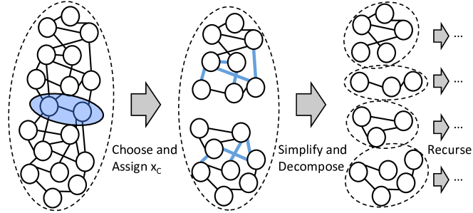
Figure 1: Visualization of RDIS decomposing the objective function. Vertices (circles) represent variables and edges connect each pair of variables in a term. Left: RDIS selects $\mathbf{x}_{C}$ (shaded oval). Middle: The function during simplification. Thick edges indicate simplifiable terms. Assigned variables are constant and have been removed. Right: The function after decomposition.

To simplify the objective function (line 9), RDIS determines which terms are simplifiable (i.e., have sufficiently small bounds) and then simplifies (approximates) these by replacing them with a constant. These terms are not passed to the recursive calls. After variables have been assigned and the function simplified, RDIS locally decomposes (line 10) the simplified function into independent sub-functions (components) that have no overlapping terms or variables and thus can be optimized independently, which is done by recursively calling RDIS on each. See Figure 1 for a visualization of this process. The recursion halts when ChooseVars selects all of $\mathbf{x}$ (i.e., $\mathbf{x}_{C}=\mathbf{x}$ and $\mathbf{x}_{U}=\varnothing$), which occurs when $\mathbf{x}$ is small enough that the subspace optimizer can optimize $f(\mathbf{x})$ directly. At this point, RDIS repeatedly calls the subspace optimizer until the stopping criterion is met, which (ideally) finds the global optimum of $f|_{\sigma^{*}_{U}}(\mathbf{x}_{C})=f(\mathbf{x})$ since $S$ is a nonconvex optimizer. The stopping criterion is user-specified, and depends on the subspace optimizer. If a multi-start descent method is used, termination occurs after a specified number of restarts, corresponding to a certain probability that the global optimum has been found. If the subspace optimizer is grid search, then the loop terminates after all values of $\mathbf{x}_{C}$ have been assigned. More subroutine details are provided in Section 4.

3 Analysis

We now present analytical results demonstrating the benefits of RDIS versus standard algorithms for nonconvex optimization. Formally, we show that RDIS explores the state space in exponentially less time than the same subspace optimizer for a class of functions that are locally decomposable, and that it will (asymptotically) converge to the global optimum. Due to space limitations, proofs are presented in Appendix A. Let the number of variables be $n$ and the number of values assigned by RDIS to $\mathbf{x}_{C}$ be $\xi(d)$, where $d$ is the size of $\mathbf{x}_{C}$. The form of $\xi(d)$ depends on the subspace optimizer, but can be roughly interpreted as the number of modes of the sub-function $f|_{\sigma^{*}_{U}}(\mathbf{x}_{C})$ to explore times a constant factor.

Proposition 1.

If, at each level, RDIS chooses $\mathbf{x}_{C}\subseteq\mathbf{x}$ of size $|\mathbf{x}_{C}|=d$ such that, for each selected value $\rho_{C}$, the simplified function $\hat{f}|_{\rho_{C}}(\mathbf{x}_{U})$ locally decomposes into $k>1$ independent sub-functions $\{\hat{f}_{i}(\mathbf{x}_{U_{i}})\}$ with equal-sized domains $\mathbf{x}_{U_{i}}$, then the time complexity of RDIS is $O(\frac{n}{d}\xi(d)^{\log_{k}{(n/d)}})$.

Note that since RDIS uses hypergraph partitioning to choose variables, it will always decompose the remaining variables $\mathbf{x}_{U}$. This is also supported by our experimental results; if there were no decomposition, RDIS would not perform any better than the baselines.

From Proposition 1, we can compute the time complexity of RDIS for different subspace optimizers. Let the subspace optimizer be grid search (GS) over a bounded domain of width $w$ with spacing $\delta$ in each dimension. Then the complexity of grid search is simply $O((w/\delta)^{n})=O(s^{n})$.

Proposition 2.

If the subspace optimizer is grid search, then $\xi(d)=(w/\delta)^{d}=s^{d}$, and the complexity of RDIS_GS is $O(\frac{n}{d}s^{d\log_{k}{(n/d)}})$.

Rewriting the complexity of grid search as $O(s^{n})=O(s^{d(n/d)})$, we see that it is exponentially worse than the complexity of RDIS_GS when decomposition occurs.

Now consider a descent method with random restarts (DR) as the subspace optimizer. Let the volume of the basin of attraction of the global minimum (the global basin) be $l^{n}$ and the volume of the space be $L^{n}$. Then the probability of randomly restarting in the global basin is $(l/L)^{n}=p^{n}$. Since the restart behavior of DR is a Bernoulli process, the expected number of restarts to reach the global basin is $r=p^{-n}$, from the shifted geometric distribution. If the number of iterations needed to reach the stationary point of the current basin is $\tau$ then the expected complexity of DR is $O(\tau p^{-n})$. If DR is used within RDIS, then we obtain the following result.

Proposition 3.

If the subspace optimizer is DR, then the expected value of $\xi(d)$ is $\tau p^{-d}$, and the expected complexity of RDIS_DR is $O(\frac{n}{d}(\tau p^{-d})^{\log_{k}{(n/d)}})$.

Rewriting the expected complexity of DR as $O(\tau{(p^{-d}})^{n/d})$ shows that RDIS_DR is exponentially more efficient than DR.

Regarding convergence, RDIS with $\epsilon=0$ converges to the global minimum given certain conditions on the subspace optimizer. For grid search, RDIS_GS returns the global minimum if the grid is finite and has sufficiently fine spacing. For gradient descent with restarts, RDIS_DR will converge to stationary points of $f(\mathbf{x})$ as long as steps by the subspace optimizer satisfy two technical conditions. The first is an Armijo rule guaranteeing sufficient decrease in $f$ and the second guarantees a sufficient decrease in the norm of the gradient (see (C1) and (C2) in Appendix A.2). These conditions are necessary to show that RDIS_DR behaves like an inexact Gauss-Seidel method Bonettini (2011), and thus each limit point of the generated sequence is a stationary point of $f(\mathbf{x})$. Given this, we can state the probability with which RDIS_DR will converge to the global minimum.

Proposition 4.

If the non-restart steps of RDIS satisfy (C1) and (C2), $\epsilon=0$, the number of variables is $n$, the volume of the global basin is $v=l^{n}$, and the volume of the entire space is $V=L^{n}$, then RDIS_DR returns the global minimum after $t$ restarts, with probability $1-(1-(v/V))^{t}$.

For $\epsilon>0$, we do not yet have a proof of convergence, even in the convex case, since preliminary analysis indicates that there are rare corner cases in which the alternating aspect of RDIS, combined with the simplification error, can potentially result in a non-converging sequence of values; however, we have not experienced this in practice. Furthermore, our experiments clearly show $\epsilon>0$ to be extremely beneficial, especially for large, highly-connected problems.

Beyond its discrete counterparts, RDIS is related to many well-known continuous optimization algorithms. If all variables are chosen at the top level of recursion, then RDIS simply reduces to executing the subspace optimizer. If one level of recursion occurs, then RDIS behaves similarly to alternating minimization algorithms (which also have global convergence results Grippo and Sciandrone (1999)). For multiple levels of recursion, RDIS has similarities to block coordinate (gradient) descent algorithms (see Tseng and Yun [2009] and references therein). However, what sets RDIS apart is that decomposition in RDIS is determined locally, dynamically, and recursively. Our analysis and experiments show that exploiting this can lead to substantial performance improvements.

4 RDIS Subroutines

In this section, we present the specific choices we’ve made for the subroutines in RDIS, but note that others are possible and we intend to investigate them in future work.

Variable Selection. Many possible methods exist for choosing variables. For example, heuristics from satisfiability may be applicable (e.g., VSIDS Moskewicz et al. (2001)). However, RDIS uses hypergraph partitioning in order to ensure decomposition whenever possible. Hypergraph partitioning splits a graph into $k$ components of approximately equal size while minimizing the number of hyperedges cut. To maximize decomposition, RDIS should choose the smallest block of variables that, when assigned, decomposes the remaining variables. This corresponds exactly to the set of edges cut by hypergraph partitioning on a hypergraph that has a vertex for each term and a hyperedge for each variable that connects the terms that variable is in (note that this is the inverse of Figure 1). RDIS maintains such a hypergraph and uses the PaToH hypergraph partitioning library Çatalyürek and Aykanat (2011) to quickly find good, approximate partitions. A similar idea was used in Darwiche and Hopkins 2001 to construct d-trees for recursive conditioning; however, they only apply hypergraph partitioning once at the beginning, whereas RDIS performs it at each level of the recursion.

While variable selection could be placed inside the loop, it would repeatedly choose the same variables because hypergraph partitioning is based on the graph structure. However, RDIS still exploits local decomposition because the variables and terms at each level of recursion vary based on local structure. In addition, edge and vertex weights could be set based on current bounds or other local information.

Value Selection. RDIS can use any nonconvex optimization subroutine to choose values, allowing the user to pick an optimizer appropriate to their domain. In our experiments, we use multi-start versions of both conjugate gradient descent and Levenberg-Marquardt, but other possibilities include Monte Carlo search, quasi-Newton methods, and simulated annealing. We experimented with both grid search and branch and bound, but found them practical only for easy problems. In our experiments, we have found it helpful to stop the subspace optimizer early, because values are likely to change again in the next iteration, making quick, approximate improvement more effective than slow, exact improvement.

Simplification and Decomposition. Simplification is performed by checking whether each term (or factor) is simplifiable and, if it is, setting it to a constant and removing it from the function. RDIS knows the analytical form of the function and uses interval arithmetic Hansen and Walster (2003) as a general method for computing and maintaining bounds on terms to determine simplifiability. RDIS maintains the connected components of a dynamic graph Holm et al. (2001) over the variables and terms (equivalent in structure to a factor or co-occurrence graph). Components in RDIS correspond exactly to the connected components in this graph. Assigned variables and simplified terms are removed from this graph, potentially inducing local decomposition.

Caching and Branch & Bound. RDIS’ similarity to model counting algorithms suggests the use of component caching and branch and bound (BnB). We experimented with these and found them effective when used with grid search; however, they were not beneficial when used with descent-based subspace optimizers, which dominate grid-search-based RDIS on non-trivial problems. For caching, this is because components are almost never seen again, due to not re-encountering variable values, even approximately. For BnB, interval arithmetic bounds tended to be overly loose and no bounding occurred. Our experience suggests that this is because the descent-based optimizer effectively focuses exploration on the minima of the space, which are typically close in value to the current optimum. However, we believe that future work on caching and better bounds would be beneficial.

5 Experimental Results

We evaluated RDIS on three difficult nonconvex optimization problems with hundreds to thousands of variables: structure from motion, a high-dimensional sinusoid, and protein folding. Structure from motion is an important problem in vision, while protein folding is a core problem in computational biology. We ran RDIS with a fixed number of restarts at each level, thus not guaranteeing that we found the global minimum. For structure from motion, we compared RDIS to that domain’s standard technique of Levenberg-Marquardt (LM) Nocedal and Wright (2006) using the levmar library Lourakis (2004), as well as to a block-coordinate descent version (BCD-LM). In protein folding, gradient-based methods are commonly used to determine the lowest energy configuration of a protein, so we compared RDIS to conjugate gradient descent (CGD) and a block-coordinate descent version (BCD-CGD). CGD and BCD-CGD were also used for the high-dimensional sinusoid. Blocks were formed by grouping contextually-relevant variables together (e.g., in protein folding, we never split up an amino acid). We also compared to ablated versions of RDIS. RDIS-RND uses a random variable selection heuristic and RDIS-NRR does not use any internal random restarts (i.e., it functions as a convex optimizer) but does have top-level restarts. In each domain, the optimizer we compare to was also used as the subspace optimizer in RDIS. All experiments were run on the same cluster. Each computer in the cluster was identical, with two 2.33GHz quad core Intel Xeon E5345 processors and 16GB of RAM. Each algorithm was limited to a single thread. Further details can be found in Appendix C.

Structure from Motion. Structure from motion is the problem of reconstructing the geometry of a 3-D scene from a set of 2-D images of that scene. It consists of first determining an initial estimate of the parameters and then performing non-linear optimization to minimize the squared error between a set of 2-D image points and a projection of the 3-D points onto camera models Triggs et al. (2000). The latter, known as bundle adjustment, is the task we focus on here. Global structure exists, since cameras interact explicitly with points, creating a bipartite graph structure that RDIS can decompose, but (nontrivial) local structure does not exist because the bounds on each term are too wide and tend to include $\infty$. The dataset used is the 49-camera, 7776-point data file from the Ladybug dataset Agarwal et al. (2010)

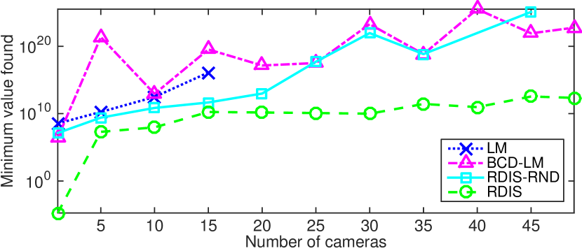
Figure 2: Minimum value found in one hour for increasing sizes of bundle adjustment problem (y-axis is log scale).

Figure 2 shows performance on bundle adjustment as a function of the size of the problem, with a log scale y-axis. Each point is the minimum error found after running each algorithm for $5$ hours. Each algorithm is given the same set of restart states, but algorithms that converge faster may use more of these. Since no local structure is exploited, Figure 2 effectively demonstrates the benefits of using recursive decomposition with intelligent variable selection for nonconvex optimization. Decomposing the optimization across independent subspaces allows the subspace optimizer to move faster, further, and more consistently, allowing RDIS to dominate the other algorithms. Missing points are due to algorithms not returning any results in the allotted time.

High-dimensional Sinusoid. The second domain is a highly-multimodal test function defined as a multidimensional sinusoid placed in the basin of a quadratic, with a small slope to make the global minimum unique. The arity of this function (i.e., the number of variables contained in each term) is controlled parametrically. Functions with larger arities contain more terms and dependencies, and thus are more challenging. A small amount of local structure exists in this problem.

In Figure 3, we show the current best value found versus time. Each datapoint is from a single run of an algorithm using the same set of top-level restarts, although, again, algorithms that converge faster use more of these. RDIS outperforms all other algorithms, including RDIS-NRR. This is due to the nested restart behavior afforded by recursive decomposition, which allows RDIS to effectively explore each subspace and escape local minima. The poor initial performance of RDIS for arities $8$ and $12$ is due to it being trapped in a local minimum for an early variable assignment while performing optimizations lower in the recursion. However, once the low-level recursions finish it escapes and finds the best minimum without ever performing a top level restart (Figure 7 in Appendix C.2 contains the full trajectories).

Protein Folding. The final domain is sidechain placement for protein folding with continuous angles between atoms. Amino acids are composed of a backbone segment and a sidechain. Sidechain placement requires setting the sidechain angles with the backbone atoms fixed. It is equivalent to finding the MAP assignment of a continuous pairwise Markov random field (cf., Yanover et al. [2006]). Significant local structure is present in this domain. Test proteins were selected from the Protein Data Bank Berman et al. (2000) with sequence length 300-600 such that the sequences of any two did not overlap by more than 30%.

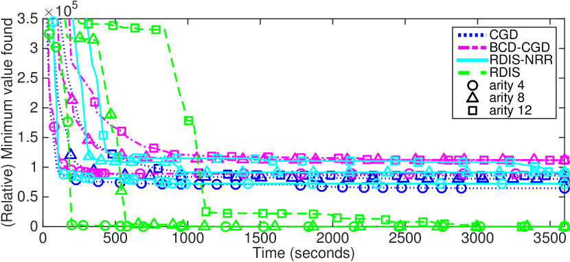
Figure 3: A comparison of the best minima found as a function of time for three different arities of the high-dimensional sinusoid.

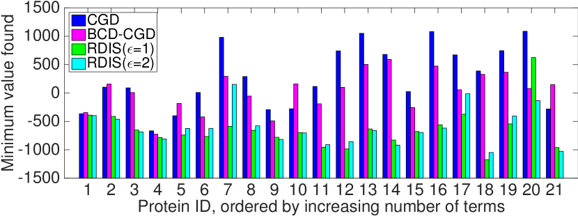
Figure 4: Minimum value (energy) found on $21$ different proteins.

Figure 4 shows the results of combining all aspects of RDIS, including recursive decomposition, intelligent variable selection, internal restarts, and local structure on a difficult problem with significant local structure. Each algorithm is run for $48$ hours on each of $21$ proteins of varying sizes. RDIS is run with both $\epsilon=1.0$ and $\epsilon=2.0$ and both results are shown on the figure. RDIS outperforms CGD and BCD-CGD on all proteins, often by a very large amount.

Figure 5 demonstrates the effect of $\epsilon$ on RDIS for protein folding. It shows the performance of RDIS-NRR as a function of $\epsilon$, where performance is measured both by minimum energy found and time taken. RDIS-NRR is used in order to remove the randomness associated with the internal restarts of RDIS, resulting in a more accurate comparison across multiple runs. Each point on the energy curve is the minimum energy found over the same $20$ restarts. Each point on the time curve is the total time taken for all $20$ restarts. As $\epsilon$ increases, time decreases because more local structure is being exploited. In addition, minimum energy actually decreases initially. We attribute this to the smoothing caused by increased simplification, allowing RDIS to avoid minor local minima in the objective function.

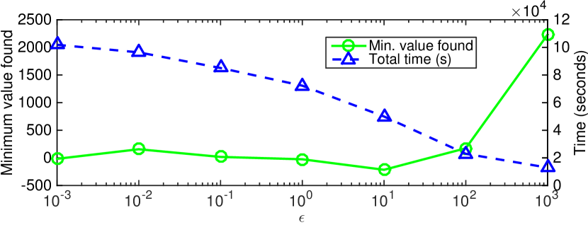
Figure 5: RDIS-NRR’s minimum energy found and total time taken versus $\epsilon$, on protein 3EEQ (ID 9). The x-axis is log scale.

6 Conclusion

This paper proposed a new approach to solving hard nonconvex optimization problems based on recursive decomposition. RDIS decomposes the function into approximately locally independent sub-functions and then optimizes these separately by recursing on them. This results in an exponential reduction in the time required to find the global optimum. In our experiments, we show that problem decomposition enables RDIS to systematically outperform comparable methods.

Directions for future research include applying RDIS to a wide variety of nonconvex optimization problems, further analyzing its theoretical properties, developing new variable and value selection methods, extending RDIS to handle hard constraints, incorporating discrete variables, and using similar ideas for high-dimensional integration.

Appendix A Analysis Details

A.1 Complexity

RDIS begins by choosing a block of variables, $\mathbf{x}_{C}$. Assuming that this choice is made heuristically using the PaToH library for hypergraph partitioning, which is a multi-level technique, then the complexity of choosing variables is linear (see Trifunović 2006, p. 81). Within the loop, RDIS chooses values for $\mathbf{x}_{C}$, simplifies and decomposes the function, and finally recurses. Let the complexity of choosing values using the subspace optimizer be $g(d)$, where $|\mathbf{x}_{C}|=d$, and let one call to the subspace optimizer be cheap relative to $n$ (e.g., computing the gradient of $f$ with respect to $\mathbf{x}_{C}$ or taking a step on a grid). Simplification requires iterating through the set of terms and computing bounds, so is linear in the number of terms, $m$. The connected components are maintained by a dynamic graph algorithm Holm et al. [2001] which has an amortized complexity of $O(\log^{2}(|V|))$ per operation, where $|V|$ is the number of vertices in the graph. Finally, let the number of iterations of the loop be a function of the dimension, $\xi(d)$, since more dimensions generally require more restarts.

Proposition 5.

If, at each level, RDIS chooses $\mathbf{x}_{C}\subseteq\mathbf{x}$ of size $|\mathbf{x}_{C}|=d$ such that, for each selected value $\rho_{C}$, the simplified function $\hat{f}|_{\rho_{C}}(\mathbf{x}_{U})$ locally decomposes into $k>1$ independent sub-functions $\{\hat{f}_{i}(\mathbf{x}_{U_{i}})\}$ with equal-sized domains $\mathbf{x}_{U_{i}}$, then the time complexity of RDIS is $O(\frac{n}{d}\xi(d)^{\log_{k}{(n/d)}})$.

Proof.

Assuming that $m$ is of the same order as $n$, the recurrence relation for RDIS is $T(n)=O(n)+\xi(d)\left[g(d)+O(m)+O(n)+O(d\log^{2}(n))+k~{}T\left(\frac{n-d}{k}\right)\right]$, which can be simplified to $T(n)=\xi(d)\left[k~{}T\left(\frac{n}{k}\right)+O(n)\right]+O(n)$. Noting that the recursion halts at $T(d)$, the solution to the above recurrence relation is then ${T(n)=c_{1}~{}\left(k~{}\xi(d)\right)^{log_{k}{(n/d)}}+c_{2}~{}n\sum_{r=0}^{log_{k}{(n/d)}-1}{\xi(d)^{r}}}$. which is $O\left((k\,\xi(d))^{\log_{k}{(n/d)}}\right)=O\left(\frac{n}{d}\xi(d)^{\log_{k}{(n/d)}}\right)$. ∎

A.2 Convergence

In the following, we refer to the basin of attraction of the global minimum as the global basin. Formally, we define a basin of attraction as follows.

Definition 2.

The basin of attraction of a stationary point $\mathbf{c}$ is the set of points $B\subseteq\mathbb{R}^{n}$ for which the sequence generated by DR, initialized at $\mathbf{x}^{0}\in B$, converges to $\mathbf{c}$.

Intuitively, at each level of recursion, RDIS with $\epsilon=0$ partitions $\mathbf{x}$ into $\left\{\mathbf{x}_{C},\mathbf{x}_{U}\right\}$, sets values using the subspace optimizer $\rho_{C}$ for $\mathbf{x}_{C}$, globally optimizes $f|_{\rho_{C}}(\mathbf{x}_{U})$ by recursively calling RDIS, and repeats. When the non-restart steps of the subspace optimizer satisfy two practical conditions (below) of sufficient decrease in (1) the objective function (a standard Armijo condition) and (2) the gradient norm over two successive partial updates, (i.e., conditions (3.1) and (3.3) of  Bonettini [2011]), then this process is equivalent to the $2$-block inexact Gauss-Seidel method (2B-IGS) described in  Bonettini [2011] (c.f.,  Grippo and Sciandrone [1999];   Cassioli et al. [2013]), and each limit point of the sequence generated by RDIS is a stationary point of $f(\mathbf{x})$, of which the global minimum is one, and reachable through restarts.

Formally, let superscript $r$ indicate the recursion level, with $0\leq r\leq d$, with $r=0$ the top, and recall that $\mathbf{x}_{U}^{(r)}=\left\{\mathbf{x}_{C}^{(r+1)},\mathbf{x}_{U}^{(r+1)}\right\}$ if there is no decomposition. The following proofs focus on the no-decomposition case for clarity; however, the extension to the decomposable case is trivial since each sub-function of the decomposition is independent. We denote applying the subspace optimizer to $f(\mathbf{x})$ until the stopping criterion is reached as $S_{*}(f,\mathbf{x})$ and a single call to the subspace optimizer as $S_{1}(f,\mathbf{x})$ and note that $S_{*}(f,\mathbf{x})$, by definition, returns the global minimum $\mathbf{x}^{*}$ and that repeatedly calling $S_{1}(f,\mathbf{x})$ is equivalent to calling $S_{*}(f,\mathbf{x})$.

For convenience, we restate conditions (3.1) and (3.3) from  Bonettini [2011] (without constraints) on the sequence $\{\mathbf{x}^{(k)}\}$ generated by an iterative algorithm on blocks $\mathbf{x}_{i}$ for $i=1,\dots,m$, respectively as

$$f(\mathbf{x}_{1}^{(k+1)},\dots,\mathbf{x}_{i}^{(k+1)},\dots,\mathbf{x}_{m}^{(k)})\leq f(\mathbf{x}_{1}^{(k+1)},\dots,\mathbf{x}_{i}^{(k)}+\lambda_{i}^{(k)}\textbf{\emph{d}}_{i}^{(k)},\dots,\mathbf{x}_{m}^{(k)}),~{}~{}~{}~{}~{}~{}~{}~{}~{}~{}~{}(C1)$$

where $\lambda_{i}^{(k)}$ is computed using Armijo line search and $\textbf{\emph{d}}_{i}^{(k)}$ is a feasible descent direction, and

$$||\nabla_{i}f(\mathbf{x}_{1}^{(k+1)},\dots,\mathbf{x}_{i}^{(k+1)},\dots,\mathbf{x}_{m}^{(k)})||\\ \leq\eta||\nabla_{i}f(\mathbf{x}_{1}^{(k+1)},\dots,\mathbf{x}_{i-1}^{(k+1)},\dots,\mathbf{x}_{m}^{(k)})||\text{*}{i=1,\dots,m}$$

$$||\nabla_{i}f(\mathbf{x}_{1}^{(k+1)},\dots,\mathbf{x}_{i}^{(k+1)},\dots,\mathbf{x}_{m}^{(k+1)})||\\ \leq\eta||\nabla_{i-1}f(\mathbf{x}_{1}^{(k+1)},\dots,\mathbf{x}_{i-1}^{(k+1)},\dots,\mathbf{x}_{m}^{(k)})||\text{*}{i=2,\dots,m}$$

$$||\nabla_{1}f(\mathbf{x}_{1}^{(k+2)},\dots,\mathbf{x}_{i}^{(k+1)},\dots,\mathbf{x}_{m}^{(k+1)})||\\ \leq\eta^{1-m}||\nabla_{m}f(\mathbf{x}_{1}^{(k+1)},\dots,\mathbf{x}_{m}^{(k+1)})||,~{}~{}~{}~{}~{}~{}~{}~{}~{}~{}~{}(C2)$$

where $\eta\in[0,1)$ is a forcing parameter. See  Bonettini [2011] for further details. The inexact Gauss-Seidel method is defined as every method that generates a sequence such that these conditions hold and is guaranteed to converge to a critical point of $f(\mathbf{x})$ when $m=2$. Let RDIS_DR refer to RDIS$(f,\mathbf{x},\mathbf{x}^{0},S=\text{DR},\epsilon=0)$.

Proposition 6.

If the non-restart steps of RDIS satisfy (C1) and (C2), $\epsilon=0$, the number of variables is $n$, the volume of the global basin is $v=l^{n}$, and the volume of the entire space is $V=L^{n}$, then RDIS_DR returns the global minimum after $t$ restarts, with probability $1-(1-(v/V))^{t}$.

Proof.

Step 1. Given a finite number of restarts, one of which starts in the global basin, then RDIS_DR, with no recursion, returns the global minimum and satisfies (C1) and (C2). This can be seen as follows.

At $r=0$, RDIS_DR chooses $\mathbf{x}_{C}^{(0)}=\mathbf{x}^{0}$ and $\mathbf{x}_{U}^{(0)}=\emptyset$ and repeatedly calls $S_{1}(f^{(0)},\mathbf{x}_{C}^{(0)})$. This is equivalent to calling $S_{*}(f^{(0)},\mathbf{x}_{C}^{(0)})=S_{*}(f,\mathbf{x})$, which returns the global minimum ${\mathbf{x}^{*}}$. Thus, RDIS_DR returns the global minimum. Returning the global minimum corresponds to a step in the exact Gauss-Seidel algorithm, which is a special case of the IGS algorithm and, by definition, satisfies (C1) and (C2).

Step 2. Now, if the non-restart steps of $S_{1}(f,\mathbf{x})$ satisfy (C1) and (C2), then RDIS_DR returns the global minimum. We show this by induction on the levels of recursion.

Base case. From Step 1, we have that RDIS_DR$(f^{(d)},\mathbf{x}^{(d)})$ returns the global minimum and satisfies (C1) and (C2), since RDIS_DR does not recurse beyond this level.
Induction step. Assume that RDIS_DR$(f^{(r+1)},\mathbf{x}^{(r+1)})$ returns the global minimum. We now show that RDIS_DR$(f^{(r)},\mathbf{x}^{(r)})$ returns the global minimum. RDIS_DR$(f^{(r)},\mathbf{x}^{(r)})$ first partitions $\mathbf{x}^{(r)}$ into the two blocks $\mathbf{x}_{C}^{(r)}$ and $\mathbf{x}_{U}^{(r)}$ and then iteratively takes the following two steps: $\rho_{C}^{(r)}\leftarrow S_{1}(f|_{\sigma^{*}_{U}}^{(r)}(\mathbf{x}_{C}^{(r)}))$ and $\rho_{U}^{(r)}\leftarrow$ RDIS_DR$(f|_{\rho_{C}}^{(r)}(\mathbf{x}_{U}))$. The first simply calls the subspace optimizer on $\rho_{C}^{(r)}$. The second is a recursive call equivalent to RDIS_DR$(f^{(r+1)},\mathbf{x}^{(r+1)})$, which, from our inductive assumption, returns the global minimum $\rho_{U}^{(r)}=\mathbf{x}_{U}^{(r)^{*}}$ of $f|_{\rho_{C}}^{(r)}(\mathbf{x}_{U})$ and satisfies (C1) and (C2). For $S_{1}(f|_{\sigma^{*}_{U}}^{(r)}(\mathbf{x}_{C}^{(r)}))$, RDIS_DR will never restart the subspace optimizer unless the sequence it is generating converges. Thus, for each restart, since there are only two blocks and both the non-restart steps of $S_{1}(f|_{\sigma^{*}_{U}}^{(r)}(\mathbf{x}_{C}^{(r)}))$ and the RDIS_DR$(f|_{\rho_{C}}^{(r)}(\mathbf{x}_{U}))$ steps satisfy (C1) and (C2) then RDIS_DR is a 2B-IGS method and the generated sequence converges to the stationary point of the current basin. At each level, after converging, RDIS_DR will restart, iterate until convergence, and repeat for a finite number of restarts, one of which will start in the global basin and thus converge to the global minimum, which is then returned.

Step 3. Finally, since the probability of RDIS_DR starting in the global basin is $(v/V)$, then the probability of it not starting in the global basin after $t$ restarts is $(1-(v/V))^{t}$. From above, we have that RDIS_DR will return the global minimum if it starts in the global basin, thus RDIS_DR will return the global minimum after $t$ restarts with probability $1-(1-(v/V))^{t}$. ∎

Appendix B RDIS Subroutine Details

B.1 Variable Selection

In hypergraph partitioning, the goal is to split the graph into $k$ components of approximately equal size while minimizing the number of hyperedges cut. Similarly, in order to maximize decomposition, RDIS should choose the smallest block of variables that, when assigned, decomposes the remaining variables. Accordingly, RDIS constructs a hypergraph $H=(V,E)$ with a vertex for each term, $\{n_{i}\in V:f_{i}\in f\}$ and a hyperedge for each variable, $\{e_{j}\in E:x_{j}\in\mathbf{x}\}$, where each hyperedge $e_{j}$ connects to all vertices $n_{i}$ for which the corresponding term $f_{i}$ contains the variable $x_{j}$. Partitioning $H$, the resulting cutset will be the smallest set of variables that need to be removed in order to decompose the hypergraph. And since assigning a variable to a constant effectively removes it from the optimization (and the hypergraph), the cutset is exactly the set that RDIS chooses on line 2.

B.2 Execution time

Variable selection typically occupies only a tiny fraction of the runtime of RDIS, with the vast majority of RDIS’ execution time spent computing gradients for the subspace optimizer. A small, but non-negligible amount of time is spent maintaining the component graph, but this is much more efficient than if we were to recompute the connected components each time, and the exponential gains from decomposition are well worth the small upkeep costs.

Appendix C Experimental Details

All experiments were run on the same compute cluster. Each computer in the cluster was identical, with two 2.33GHz quad core Intel Xeon E5345 processors and 16GB of RAM. Each algorithm was limited to a single thread.

C.1 Structure from Motion

In the structure from motion task (bundle adjustment Triggs et al. [2000]), the goal is to minimize the error between a dataset of points in a 2-D image and a projection of fitted 3-D points representing a scene’s geometry onto fitted camera models. The variables are the parameters of the cameras and the positions of the points and the cameras. This problem is highly-structured in a global sense: cameras only interact explicitly with points, creating a bipartite graph structure that RDIS is able to exploit. The dataset used is the 49-camera, 7776-point data file from the Ladybug dataset Agarwal et al. [2010], where the number of points is scaled proportionally to the number of cameras used (i.e., if half the cameras were used, half of the points were included). There are $9$ variables per camera and $3$ variables per point.

C.2 Highly Multimodal Test Function

The test function is defined as follows. Given a height $h$, a branching factor $k$, and a maximum arity $a$, we define a complete $k$-ary tree of variables of the specified height, with $x_{0}$ as the root. For all paths $p_{j}\in P$ in the tree of length $l_{j}\leq a$, with $l_{j}$ even, we define a term $t_{p_{j}}=\prod_{x_{i}\in p_{j}}\sin(x_{i})$. The test function is $f_{h,k,a}(x_{0},\dots,x_{n})=\sum_{i=1}^{n}c_{0}x_{i}+c_{1}x_{i}^{2}+c_{2}\sum_{P}t_{p_{j}}$. The resulting function is a multidimensional sinusoid placed in the basin of a quadratic function parameterized by $c_{1}$, with a linear slope defined by $c_{0}$. The constant $c_{2}$ controls the amplitude of the sinusoids. For our tests, we used $c_{0}=0.6,c_{1}=0.1,$ and $c_{2}=12$. A 2-D example of this function is shown in Figure 6. We used a tree height of $h=11$, with branching factor $k=2$, resulting in a function of $4095$ variables. We evaluated each of the algorithms on functions with terms of arity $a\in\{4,8,12\}$, where a larger arity defines more complex dependencies between variables as well as more terms in the function. The functions for the three different arity levels had 16372, 24404, and 30036 terms, respectively.

Figure 7 shows the value of the current state for each algorithm over its entire execution. These are the trajectories for Figure 3 of the main paper.

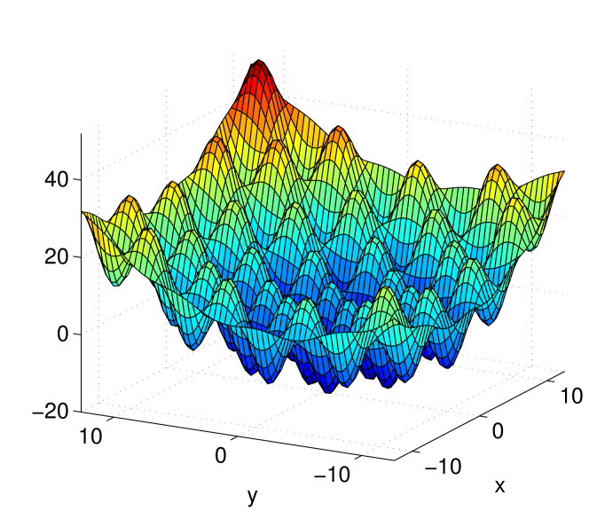
Figure 6: A 2-D example of the highly multimodal test function.

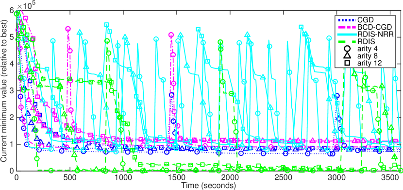
Figure 7: Trajectories on the test function for the data in Figure 3 in the main paper. Sharp rises show restarts. Notably, RDIS-NRR restarts much more often than the other algorithms because decomposition allows it to move through the space much more efficiently. Without internal restarting it gets stuck at the same local minima as BCD-CGD and CGD. For arity 12, RDIS never performs a full restart and still finds the best minimum, despite using the same initial point as the other algorithms.

C.3 Protein Folding

C.3.1 Problem details

Protein folding Anfinsen [1973]; Baker [2000] is the process by which a protein, consisting of a long chain of amino acids, assumes its functional shape. The computational problem is to predict this final conformation given a known sequence of amino acids. This requires minimizing an energy function consisting mainly of a sum of pairwise distance-based terms representing chemical bonds, hydrophobic interactions, electrostatic forces, etc., where, in the simplest case, the variables are the relative angles between the atoms. The optimal state is typically quite compact, with the amino acids and their atoms bonded tightly to one another and the volume of the protein minimized. Each amino acid is composed of a backbone segment and a sidechain, where the backbone segment of each amino acid connects to its neighbors in the chain, and the sidechains branch off the backbone segment and form bonds with distant neighbors. The sidechain placement task is to predict the conformation of the sidechains when the backbone atoms are fixed in place.

Energies between amino acids are defined by the Lennard-Jones potential function, as specified in the Rosetta protein folding library Leaver-Fay et al. [2011]. The basic form of this function is $E_{LJ}(r)=\frac{A}{r^{12}}-\frac{B}{r^{6}}$, where $r$ is the distance between two atoms and $A$ and $B$ are constants that vary for different types of atoms. The Lennard-Jones potential in Rosetta is modified slightly so that it behaves better when $r$ is very large or very small. The full energy function is $E(\phi)=\sum_{\phi}E_{jk}(R_{j}(\raisebox{2.0pt}{$\chi$}_{j}),R_{k}(\raisebox{2.0pt}{$\chi$}_{k}))$, where $R_{j}$ is an amino acid (also called a residue) in the protein, $\phi$ is the set of all torsion angles, and $\phi_{i}\in\raisebox{2.0pt}{$\chi$}_{j}$ are the angles for $R_{j}$. Each residue has between zero and four torsion angles that define the conformation of its sidechain, depending on the type of amino acid. The terms $E_{jk}$ compute the energy between pairs of residues as $E_{jk}=\sum_{a_{j}}\sum_{a_{k}}E_{LJ}(r(a_{j}(\raisebox{2.0pt}{$\chi$}_{j}),a_{k}(\raisebox{2.0pt}{$\chi$}_{k})))$, where $a_{j}$ and $a_{k}$ refer to the positions of the atoms in residues $j$ and $k$, respectively, and $r(a_{j},a_{k})$ is the distance between the two atoms. The torsion angles define the positions of the atoms through a series of kinematic relations, which we do not detail here.

The smallest (with respect to the number of terms) protein (ID 1) has $131$ residues, $2282$ terms, and $257$ variables, while the largest (ID 21) has $440$ residues, $9380$ terms, and $943$ variables. The average number of residues, terms, and variables is $334$, $7110$, and $682$, respectively. The proteins with their IDs from the paper are as follows: (1) 4JPB, (2) 4IYR, (3) 4M66, (4) 3WI4, (5) 4LN9, (6) 4INO, (7) 4J6U, (8) 4OAF, (9) 3EEQ, (10) 4MYL, (11) 4IMH, (12) 4K7K, (13) 3ZPJ, (14) 4LLI, (15) 4N08, (16) 2RSV, (17) 4J7A, (18) 4C2E, (19) 4M64, (20) 4N4A, (21) 4KMA.

References

- Agarwal et al. [2010] Sameer Agarwal, Noah Snavely, Steven M. Seitz, and Richard Szeliski. Bundle adjustment in the large. In Kostas Daniilidis, Petros Maragos, and Nikos Paragios, editors, Computer Vision ECCV 2010, volume 6312 of Lecture Notes in Computer Science, pages 29–42. Springer Berlin Heidelberg, 2010.
- Anfinsen [1973] Christian B. Anfinsen. Principles that govern the folding of protein chains. Science, 181(4096):223–230, 1973.
- Bacchus et al. [2009] Fahiem Bacchus, Shannon Dalmao, and Toniann Pitassi. Solving #SAT and Bayesian Inference with Backtracking Search. Journal of Artificial Intelligence Research, 34:391–442, 2009.
- Baker [2000] David Baker. A surprising simplicity to protein folding. Nature, 405:39–42, 2000.
- Bayardo Jr. and Pehoushek [2000] Roberto J. Bayardo Jr. and Joseph Daniel Pehoushek. Counting models using connected components. In Proceedings of the Seventeenth National Conference on Artificial Intelligence, pages 157–162, 2000.
- Berman et al. [2000] Helen M. Berman, John Westbrook, Zukang Feng, Gary Gilliland, T. N. Bhat, Helge Weissig, Ilya N. Shindyalov, and Philip E. Bourne. The protein data bank. Nucleic Acids Research, 28(1):235–242, 2000.
- Bonettini [2011] Silvia Bonettini. Inexact block coordinate descent methods with application to non-negative matrix factorization. IMA Journal of Numerical Analysis, 31(4):1431–1452, 2011.
- Cassioli et al. [2013] A Cassioli, D Di Lorenzo, and M Sciandrone. On the convergence of inexact block coordinate descent methods for constrained optimization. European Journal of Operational Research, 231(2):274–281, 2013.
- Çatalyürek and Aykanat [2011] Ümit Çatalyürek and Cevdet Aykanat. PaToH (partitioning tool for hypergraphs). In David Padua, editor, Encyclopedia of Parallel Computing, pages 1479–1487. Springer US, 2011.
- Darwiche and Hopkins [2001] Adnan Darwiche and Mark Hopkins. Using recursive decomposition to construct elimination orders, jointrees, and dtrees. In Symbolic and Quantitative Approaches to Reasoning with Uncertainty, pages 180–191. Springer, 2001.
- Darwiche [2001] Adnan Darwiche. Recursive conditioning. Artificial Intelligence, 126(1-2):5–41, 2001.
- Davis et al. [1962] Martin Davis, George Logemann, and Donald Loveland. A machine program for theorem-proving. Communications of the ACM, 5(7):394–397, 1962.
- De Moura and Bjørner [2011] Leonardo De Moura and Nikolaj Bjørner. Satisfiability modulo theories: Introduction and applications. Communications of the ACM, 54(9):69–77, September 2011.
- Griewank and Toint [1981] Andreas Griewank and Philippe L. Toint. On the unconstrained optimization of partially separable functions. Nonlinear Optimization, 1982:247–265, 1981.
- Grippo and Sciandrone [1999] Luigi Grippo and Marco Sciandrone. Globally convergent block-coordinate techniques for unconstrained optimization. Optimization Methods and Software, 10(4):587–637, 1999.
- Hansen and Walster [2003] Eldon Hansen and G. William Walster. Global optimization using interval analysis: revised and expanded, volume 264. CRC Press, 2003.
- Holm et al. [2001] Jacob Holm, Kristian De Lichtenberg, and Mikkel Thorup. Poly-logarithmic deterministic fully-dynamic algorithms for connectivity, minimum spanning tree, 2-edge, and biconnectivity. Journal of the ACM (JACM), 48(4):723–760, 2001.
- Leaver-Fay et al. [2011] Andrew Leaver-Fay, Michael Tyka, Steven M Lewis, Oliver F Lange, James Thompson, Ron Jacak, Kristian Kaufman, P Douglas Renfrew, Colin A Smith, Will Sheffler, et al. ROSETTA3: an object-oriented software suite for the simulation and design of macromolecules. Methods in Enzymology, 487:545–574, 2011.
- Lourakis [2004] M.I.A. Lourakis. levmar: Levenberg-Marquardt nonlinear least squares algorithms in C/C++. http://www.ics.forth.gr/~lourakis/levmar/, 2004.
- Moskewicz et al. [2001] Matthew W. Moskewicz, Conor F. Madigan, Ying Zhao, Lintao Zhang, and Sharad Malik. Chaff: Engineering an efficient sat solver. In Proceedings of the 38th annual Design Automation Conference, pages 530–535. ACM, 2001.
- Neumaier et al. [2005] Arnold Neumaier, Oleg Shcherbina, Waltraud Huyer, and Tam s Vink . A comparison of complete global optimization solvers. Mathematical Programming, 103(2):335–356, 2005.
- Nocedal and Wright [2006] Jorge Nocedal and Stephen J Wright. Numerical Optimization. Springer, 2006.
- Sang et al. [2004] Tian Sang, Fahiem Bacchus, Paul Beame, Henry A. Kautz, and Toniann Pitassi. Combining component caching and clause learning for effective model counting. Seventh International Conference on Theory and Applications of Satisfiability Testing, 2004.
- Sang et al. [2005] Tian Sang, Paul Beame, and Henry Kautz. Performing Bayesian inference by weighted model counting. In Proceedings of the Twentieth National Conference on Artificial Intelligence (AAAI-05), volume 1, pages 475–482, 2005.
- Schoen [1991] Fabio Schoen. Stochastic techniques for global optimization: A survey of recent advances. Journal of Global Optimization, 1(3):207–228, 1991.
- Trifunović [2006] Aleksandar Trifunović. Parallel algorithms for hypergraph partitioning. Ph.D., University of London, February 2006.
- Triggs et al. [2000] Bill Triggs, Philip F. McLauchlan, Richard I. Hartley, and Andrew W. Fitzgibbon. Bundle adjustment – a modern synthesis. In Vision Algorithms: Theory and Practice, pages 298–372. Springer, 2000.
- Tseng and Yun [2009] Paul Tseng and Sangwoon Yun. A coordinate gradient descent method for nonsmooth separable minimization. Mathematical Programming, 117(1-2):387–423, 2009.
- Yanover et al. [2006] Chen Yanover, Talya Meltzer, and Yair Weiss. Linear programming relaxations and belief propagation – an empirical study. The Journal of Machine Learning Research, 7:1887–1907, 2006.