Non-conservative Forces via Quantum Reservoir Engineering

Abstract

A systematic approach is given for engineering dissipative environments that steer quantum wavepackets along desired trajectories. The methodology is demonstrated with several illustrative examples: environment-assisted tunneling, trapping, effective mass assignment and pseudo-relativistic behavior. Non-conservative stochastic forces do not inevitably lead to decoherence – we show that purity can be well-preserved. These findings highlight the flexibility offered by non-equilibrium open quantum dynamics.

I Introduction

Throughout its short history, the control of quantum systems has predominantly been implemented using conservative forces, e.g., manipulating quantum phenomena in Hamiltonian systems via dipole coupling with laser or microwave pulses. This may seem surprising given the widespread use of non-conservative forces in other control applications – consider the wind (sailing vessels, windmills) and friction (mechanical brakes). The historical focus on conservative forces is, perhaps, best explained by the widely held belief that immersing a quantum system into a complex environment inevitably destroys its quantum dynamical features. The monopoly of conservative forces in quantum control is now being challenged by quantum reservoir engineering (QRE) Poyatos et al. (1996); Verstraete et al. (2009); Fedortchenko et al. (2014); Kurizki et al. (2015); Kienzler et al. (2015); Pan et al. (2016); Rouchon (2014). In particular, it has been shown that it is possible to preserve and even enhance the quantum dynamical features of a system by judiciously coupling the system to a dissipative environment. Applications of quantum reservoir engineering include amplification Metelmann and Clerk (2014), nonreciprocal photon transmission Metelmann and Clerk (2015, 2017), photon blockade Miranowicz et al. (2014), efficient photoinduced charge separation in solar energy conversion Zhdanov and Seideman (2015), binding of atoms Lemeshko and Weimer (2013); Wüster (2017), inducing phase transitions Kaczmarczyk et al. (2016); Weimer (2016); Overbeck et al. (2017), implementation of quantum gates Albert et al. (2016); Ticozzi and Viola (2017); Arenz et al. (2016, 2017), and the generation of entangled Cheng et al. (2016); Liu et al. (2016); Zippilli et al. (2015); Yang et al. (2015); Mirza (2015); Arenz et al. (2013), squeezed Kronwald et al. (2013); Woolley and Clerk (2014); Grimsmo et al. (2016), and other exotic Koga and Yamamoto (2012); Holland et al. (2015); Asjad and Vitali (2014); Chestnov et al. (2016) quantum states.

In this Letter, we provide a systematic approach for engineering dissipative environments that steer quantum wavepackets along desired trajectories as defined by the following equations:

$$\mathop{\frac{d}{dt}}{\mathop{\langle\hat{x}\rangle}\nolimits}{=}\mathop{\langle G(\hat{p})\rangle}\nolimits,$$ (1a)

$$\mathop{\frac{d}{dt}}{\mathop{\langle\hat{p}\rangle}\nolimits}{=}\mathop{\langle F(\hat{x})\rangle}\nolimits.$$ (1b)

Here, $\mathop{\langle\hat{x}\rangle}\nolimits$ and $\mathop{\langle\hat{p}\rangle}\nolimits$ denote the wavepacket’s mean position and momentum. The environments obtained not only enhance desired quantum properties, but can also be made to preserve the purity of the underlying quantum system. Equations (1) with various functions $G$ and $F$ embrace a plethora of quantum behaviors; we provide several illustrative examples. We first consider compensating for a potential barrier in the case of quantum tunneling and then mimicking a potential to trap a wave packet at a desired location. We also consider more exotic applications such as changing the effective mass of a quantum particle and emulating relativistic effects. The scope of our analysis is restricted to Markovian environments modeled within the Lindblad formalism. We also discuss possible laboratory realizations of the Lindblad operators for specific examples.

II Formal analysis

For definiteness, assume that the system of interest is a one-dimensional particle of mass $m$ moving in a potential $U(x)$. Our objective is to dissipatively couple the system to $K+N$ baths in such a way that the average particle localization in phase space will follow Eqs. (1) for given, desirable, $G(\hat{p})$ and $F(\hat{x})$. Assuming Markovian system-bath interactions, the system state (described by the density matrix $\hat{\rho}$) evolves according to the Lindblad master equation

$$\frac{\,\mathrm{d}\hat{\rho}}{\,\mathrm{d}t} =-\frac{i}{\hbar}[\hat{H},\hat{\rho}]+\sum_{k{=}1}^{K}\mathcal{D}_{\hat{A}_{k}}[\hat{\rho}]+\sum_{n{=}1}^{N}\mathcal{D}_{\hat{B}_{n}}[\hat{\rho}],$$ (2)

where $\hat{H}$ is a given system Hamiltonian

$$\hat{H} =\frac{1}{2m}{\hat{p}}^{2}+U(\hat{x}),$$ (3)

and the effect of the bath is represented via the operators $\hat{A}_{k}$, $\hat{B}_{n}$ as

$$\mathcal{D}_{\hat{A}}[\hat{\rho}] =\frac{1}{\hbar}\Big{(}\hat{A}\hat{\rho}\hat{A}^{\dagger}-\frac{1}{2}\hat{\rho}\hat{A}^{\dagger}\hat{A}-\frac{1}{2}\hat{A}^{\dagger}\hat{A}\hat{\rho}\Big{)}.$$ (4)

Under these assumptions, the control problem reduces to determining suitable forms for the operators $\hat{A}_{k}$, $\hat{B}_{n}$ and providing physical evidence that the corresponding environments can be engineered in the laboratory. Using Operational Dynamical Modeling Bondar et al. (2012, 2016) the following expressions for $\hat{A}_{k}=A_{k}(\hat{x})$ and $\hat{B}_{n}=B_{n}(\hat{p})$ are obtained:

$$A_{k}(x)=\> R_{k}(x)\exp\left({i\int\frac{f_{k}(x)}{R_{k}^{2}(x)}\,\mathrm{d}x}\right),$$ (5a)

$$B_{n}(p)=\> S_{n}(p)\exp\left({-i\int\frac{g_{n}(p)}{S_{n}^{2}(p)}\,\mathrm{d}p}\right).$$ (5b)

Here, $$f_{k}(x) g_{k}(p) R_{k}(x) S_{k}(p)$$, , , and denote arbitrary real valued functions such that

$$\sum_{k=1}^{K}f_{k}(x){=}F(x){+}\mathop{\frac{dU(x)}{dx}};~{}~{}\sum_{n{=}1}^{N}g_{n}(p){=}G(p){-}\frac{p}{m}.$$ (5c)

Note that Eqs. (1) are satisfied regardless of the initial state. To provide insight into the physical nature of environments that implement (5), we now consider several illustrative examples. Unless stated otherwise, atomic units (a.u.), $\hbar=m_{e}=|e|=1$, are used throughout.

III Environmentally assisted quantum tunneling

It is common knowledge that cycling uphill is much easier with assistance from a tailwind. Similarly, a “polarized electron wind” can be used to enhance tunneling rates for an atomic wavepacket approaching a potential barrier $U(\hat{x})$ (see Fig. 1). If non-conservative forces are engineered so as to cancel the potential forces of the system, then dynamics similar to those of a free particle can be obtained. Consider Eqs. (1) and choose $G(p){=}\frac{p}{m}$ and $F(\hat{x}){=}0$. These dynamics can be obtained with the following choice of environmental operators $A_{\pm}$, which satisfy (5) for the case $K=2$, $N=0$, and $R_{1}=R_{2}=C$ where $C$ is a constant:

$$A_{\pm}{=}Ce^{\pm\frac{2i}{\hbar}\int{{\tilde{p}_{\pm}(x)dx}}},$$ (6a)

where the functions $$\tilde{p}_{\pm}(x)$$ obey the relation

$$\tilde{p}_{+}(x){-}\tilde{p}_{-}(x){=}\tfrac{\hbar}{2C^{2}}\tfrac{\,\mathrm{d}U(x)}{\,\mathrm{d}x}.$$ (6b)

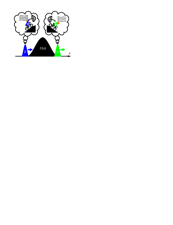
Figure 1: Environment assisted quantum tunneling resembles cycling with an umbrella: The environment action is qualitatively similar to tailwind (headwind) when going uphill (downhill). The net effect is a reduction of the back-scattering probability with minimal side effects on the wavepacket parameters.

Inspired by the wind analogy, we now propose a physical implementation of the environment (6). Consider a quantum probe that is an atom of mass $m$ in the non-degenerate ground electronic state with electric polarizability $\alpha$, zero angular momentum, and negligible magnetic polarizability. Suppose that the motion of the probe along the $\vec{\epsilon}_{x}$-axis is impeded by an effective barrier $U(x)=-\alpha{\cal E}(x)^{2}/4$ created by an off-resonant, blue-detuned ($\alpha{<}0$) laser field ${\vec{\epsilon}}_{x}\mathcal{E}(x)\cos(\omega(t-{z}/{c}))$. In the presence of a static magnetic field of the form ${\vec{\epsilon}}_{z}{\cal B}(x)$, the desired dissipative environment can be created by two counterpropagating electron jets, in which the electrons have opposite magnetic moments $\hat{\mu}_{s}{=}{\pm}\hat{\sigma}_{z}\mu_{\mathrm{B}}$, incident velocities ${\pm}{\vec{\epsilon}}_{x}\frac{p_{0}}{m_{\mathrm{e}}}$, and fluxes ${\pm}{\vec{\epsilon}}_{x}j$ (here $\mu_{\mathrm{B}}$ is the Bohr magneton). The resulting electron recoils create an effective pressure on the probe. Note that without a magnetic field, the mean impacts of both jets would mutually compensate each other. However, when a magnetic field is applied, the opposite electron spin polarizations of the jets break this symmetry resulting in a nonzero net force on the probe.

To quantitatively describe this effect, we assume that i) the electron flux $j$ is low enough to neglect multiple scattering of electrons, ii) all interactions of electrons with the probe can be modeled as ideal elastic backscattering events, iii) the incident electron velocity ${p_{0}}/{m_{\mathrm{e}}}$ is much larger than the characteristic velocities of the probe, and iv)

$$p_{0}{\gg}\sqrt{2\mu_{\mathrm{B}}m_{\mathrm{e}}|{\cal B}(x)|}.$$ (7)

The inequality (7) allows the wavefunctions of incident electrons in the jets to be modeled semiclassically as

$$\psi_{\pm}{\propto}\frac{e^{\frac{\pm i}{\hbar}\int\tilde{p}_{\pm}(x)\,\mathrm{d}x}}{\tilde{p}_{\pm}(x)},~{}~{}\tilde{p}_{\pm}(x){=}\sqrt{p_{0}^{2}\pm 2\mu_{\mathrm{B}}m_{\mathrm{e}}{\cal B}(x)}.$$ (8)

In the case of $C=\sqrt{\hbar\tilde{\sigma}j}$ where $\tilde{\sigma}$ is the scattering cross section, Eqs. (2) and (6a) describe the “wind effect” of the electron jets on the probe. Note that $C^{2}$ is proportional to the number of electron scatterings in a given time interval. Under the assumption of Poissonian statistics, the standard deviation over the same time interval of the force exerted by the collisions is expected to be proportional to $Cp_{0}$. This parameter will be used below to elucidate physical mechanisms. Finally, Eqs. (6b) and (8) determine the magnetic field profile required for effectively barrierless propagation:

$${\cal B}(x) =\frac{\hbar}{16\mu_{\mathrm{B}}m_{\mathrm{e}}C^{4}}{\frac{\,\mathrm{d}U(x)}{\,\mathrm{d}x}\sqrt{16{p_{0}}^{2}C^{4}-\left(\hbar\frac{\,\mathrm{d}U(x)}{\,\mathrm{d}x}\right)^{2}}}.$$ (9)

The character of the system-environment coupling is determined by the momenta $p_{\pm}$ of the incident electrons. For small magnitudes of $|p_{\pm}|$, large collision rates are required to create sufficient non-conservative forces to oppose the potential forces. In this case, the overall effect of the collisions can be represented as an effective pressure, and the dissipative term in (2) in the limit $C{\to}\infty$, $|p_{\pm}|{\to}0$ can be represented as an effective Hamiltonian, $\hat{H}_{\mathrm{eff}}=-U(\hat{x})$, which cancels the potential barrier $U(x)$ and results in entirely coherent (essentially free-particle) dynamics. On the other hand, large $|p_{\pm}|$ corresponds to the shot noise limit where strong but rare collisions produce highly fluctuating stochastic environmental forces. This leads to rapid wavepacket decoherence and a reduction in tunneling probabilities. These effects can be seen in Fig. 2, which depicts simulation results for a hydrogen-like atom ($m{=}1837m_{e}$ where $m_{e}$ is electron mass) tunneling through a Gaussian potential barrier in the presence of an engineered environment as described by Eqs. (2), (6), and (8). In all cases, Eqs. (1) are satisfied. For small values of $|p_{\pm}|$, high tunneling rates and purity are achieved for the atomic quantum state after interaction with the barrier. However, above a critical $|p_{\pm}|$ (which depends on the standard deviation of the environmental force $Cp_{0}$), the tunneling probability and purity dramatically degrade; this corresponds to the shot noise regime.

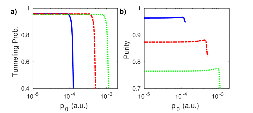
Figure 2: The transmission probability (a) and purity (b) for a Gaussian atomic wavepacket tunneling through a potential barrier in the presence of electron jets [Eqs. (2),(6),(8) and (9)] as a function of electron momentum $p_{0}$. In each case the wavepacket has initial mean kinetic energy $K_{0}=0.0068$ (a.u.) and the potential barrier is $U(x)=2K_{0}e^{-x^{2}/2}$. The solid blue, dash-dotted red, and dotted green curves correspond to incident electron energy fluctuations $Cp_{0}=5\times 10^{-4}$, $10^{-3}$ and $1.5\times 10^{-3}$ (a.u.) respectively. The right-most points of the curves in panel (b) correspond to the case when inequality (7) turns into equality.

One can observe slight increases in the purity prior to the rapid falling away in each of the curves in Fig. 2(b). These peaks correspond to a transitional regime wherein the tunneling rates are starting to degrade [see Fig. 2(a)] and reflection from the barrier becomes noticeable ($\propto 10\%$). Furthermore, the inequality (7) is only marginally satisfied; the observed purity increase may be an artifact of the semi-classical approximation (8).

The ability of environmental coupling to enhance tunneling rates has been previously recognized. Under certain physical conditions, a metastable quantum system submerged into a low temperature environment decays, exciting directional bath modes such that the quantum system acquires kinetic energy which in turn assists under the barrier motion Leggett (1984); Grabert et al. (1984); Pollak (1986); Leggett (1996). In particular, an atom can acquire an extra momentum kick, facilitating tunneling by spontaneously emitting a photon. This mechanism has been systematically explored in Refs. Japha and Kurizki (1996); Schaufler et al. (1999) and yielded Zeno and anti-Zeno quantum control schemes Barone et al. (2004). In these schemes the incident wavepackets undergo destructive spontaneous dissipative changes. However, in our example the enhanced tunneling is achieved without destroying the state purity, as can be seen from Fig. 2. It is noteworthy that environmentally assisted tunneling was recently experimentally demonstrated in lithium niobate Somma et al. (2014).

IV Dissipative traps

The same strategy can also be used to trap an atom; by setting $U(x){=}{-}U_{\text{eff}}(x)$ in Eq. (9) the environment will mimic the potential $U_{\text{eff}}(x)$. Figure. 3 depicts simulation results for a hydrogen atom immersed in trapping environments with different standard deviations of the environmental force $Cp_{0}$. As in the tunneling case, larger values for $Cp_{0}$ for a given $p_{0}$ cause additional heating. This deteriorates the trapping via purity losses and wavepacket spreading. Nevertheless, one can see that for each of the cases depicted the environmentally trapped wavepacket remains more spatially localized than the free wavepacket. These results suggest that the optimal strategy for trapping a particle is to use jets with the smallest $Cp_{0}$ for which (7) is satisfied.

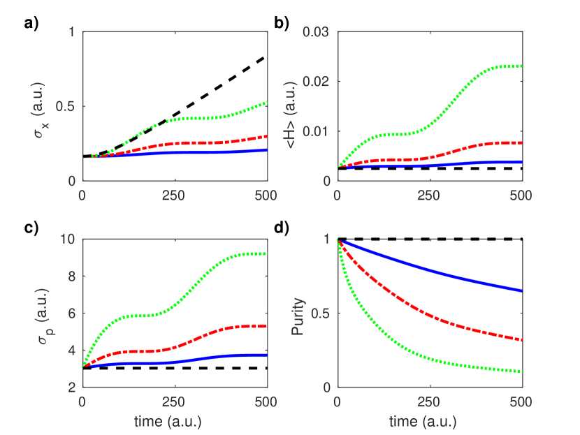
Figure 3: The spreading in position (a), increase in energy (b), spreading in momentum (c), and decrease in purity (d) for an atomic wavepacket initially in the ground state of a harmonic oscillator [$U(x)=\frac{1}{2}m(0.01x)^{2}$]. The solid blue, dash-dotted red, and dotted green curves correspond to the incident electrons’ energy fluctuations $Cp_{0}=0.05$, $0.1$ and $0.2$ (a.u.) respectively. In each case $p_{0}=10^{-4}$ a.u. Results for a free (i.e., $C=0$, $U{=}0$) wavepacket (dashed black) are shown for comparison.

It was shown in Ref. Lemeshko and Weimer (2013) that non-conservative forces between atoms can lead to binding, even when the potential interaction is repulsive.

V Exotic applications

We have demonstrated that non-conservative forces can effectively mimic desired conservative interactions, however, the utility of such forces is much wider. Non-conservative forces can also be used to obtain modifications $G(p)$ to the dispersion relationship (1a) – note that such modifications cannot be implemented via conservative forces. We consider two applications for such modifications: tuning the effective mass of a quantum particle and emulating relativistic effects.

Consider a quantum particle of mass $m$ in a potential $U(x)$. The particle will exhibit an effective mass $M$ when immersed in an environment described by the dissipator $\mathcal{D}_{B}$ [as in Eq. (2)] with

$$B(p)=C\exp\left[-\frac{i(m-M)p^{2}}{2mMC^{2}}\right].$$ (10)

That is, the system dynamics will satisfy the constraints

$$\frac{\,\mathrm{d}\;}{\,\mathrm{d}t}\langle\hat{x}\rangle=\frac{1}{M}\langle\hat{p}\rangle,\quad\frac{\,\mathrm{d}}{\,\mathrm{d}t}\langle\hat{p}\rangle=-\left\langle\frac{\,\mathrm{d}U(\hat{x})}{\,\mathrm{d}\hat{x}}\right\rangle.$$ (11)

Figure 4 depicts simulation results: the particle of mass $m$ in the environment (10) evolves in excellent agreement with an environment-free particle of mass $M$.

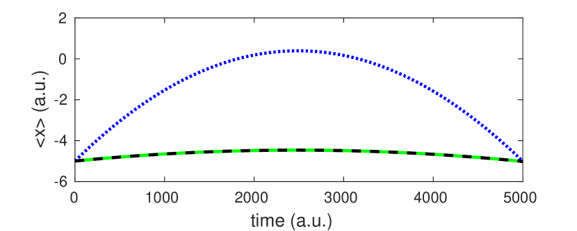
Figure 4: The expectation value of the position as a function of time for a hydrogen atom in a ramp potential $U(x)=3.2\times 10^{-3}x$ a.u. The dotted blue curve depicts the environment-free case. The solid green curve depicts the atom in an environment (10) [$M=10m$, $C=0.1$] engineered to give an effective mass ten times the proton mass $m$. The dynamics of the hydrogen atom with environmentally induced effective mass $M$ coincide with those of an environment-free particle of mass $M$ (dashed black).

The effective mass approximation is ubiquitously used to describe the motion of a quantum particle in the periodic field of a solid. Recently, a negative effective mass was experimentally achieved Khamehchi et al. (2017). An atom interacting with the standing wave of a single photon in the cavity also acquires an effective mass Larson et al. (2005). We conjecture that environmentally induced mass can emerge for an atom elastically scattering off incoherent light seeded into a cavity.

We now turn our attention to environmentally induced quasi-relativistic behaviour. Once again, consider a quantum particle of mass $m$ in a potential $U(x)$. Suppose we wish the system dynamics to satisfy the constraints

$$\frac{\,\mathrm{d}\;}{\,\mathrm{d}t}\langle\hat{x}\rangle=\left\langle\frac{\hat{p}}{\sqrt{m^{2}+\hat{p}^{2}/c^{2}}}\right\rangle,\quad\frac{\,\mathrm{d}}{\,\mathrm{d}t}\langle\hat{p}\rangle=-\left\langle\frac{\,\mathrm{d}U(\hat{x})}{\,\mathrm{d}\hat{x}}\right\rangle.$$ (12)

This can be achieved with an environment described by the dissipator $\mathcal{D}_{B}$ with

$$B(p)=C\exp\left[\frac{i}{C^{2}}\left(\frac{p^{2}}{2m}-c\sqrt{m^{2}c^{2}+p^{2}}\right)\right].$$ (13)

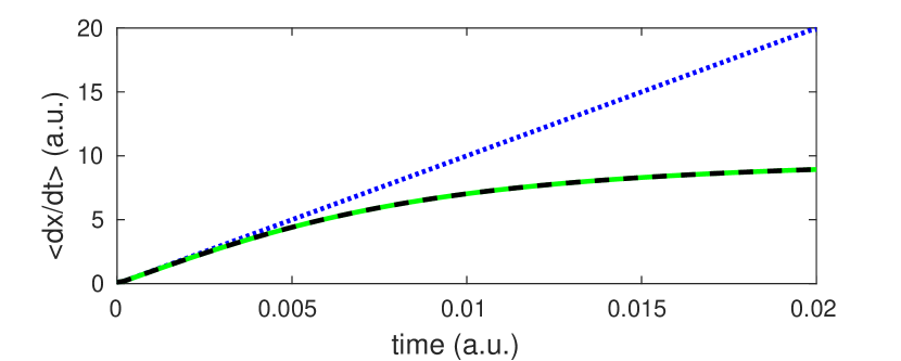
Figure 5: The expectation value of the velocity as a function of time for an electron in a ramp potential $U(x)=-10^{3}x$ a.u. The dotted blue curve depicts the environment-free case. The solid green curve depicts the electron in an environment (13) ($C=20$ a.u.) engineered to induce quasi-relativistic behaviour with the speed of light chosen to be 7% of the speed of light in vacuum. The environmentally induced quasi-relativistic behaviour coincides with that of an environment-free relativistic electron with Hamiltonian $\hat{H}_{\mathrm{rel}}=\sqrt{c^{2}\hat{p}^{2}+c^{4}}+U(\hat{x})$; $c=10$ (dashed black).

Figure 5 depicts simulation results confirming that the chosen environment induces quasi-relativistic behaviour for an arbitrarily small speed of light. In particular, the environment mimics the effect of time dilation as the particle velocity approaches the chosen speed of light.

The dispersion relation emerges as an effective description of the self-interaction of a bare quantum particle with a larger system with some characteristic symmetry. Generalizing the logic of Ref. Larson et al. (2005), we conjecture that tailoring the spectral transmission characteristics of a cavity and employing multi-color electromagnetic radiation with specific photon statistics should provide access to a large class of dispersion relations.

Outlook. Physicists, chemists, and engineers are increasingly looking for new ways to manipulate quantum systems – non-conservative environments provide one such resource. We give a systematic approach for designing such environments to steer wavepackets along desired trajectories. The method is demonstrated via several examples: enhancing quantum tunneling, trapping particles, inducing effective mass, and emulating relativistic effects. The proposed dissipators not only enhance desired quantum properties, they can be engineered to do so while preserving the purity of the underlying system. A distinct feature of our method is that for a given $F$ and $G$, the resulting dynamics always satisfy Eqs. (1), irrespective of the initial state.

Finally, note that $F(x)$ in Eq. (1b) is the sum of the potential force $-\,\mathrm{d}U(x)/\,\mathrm{d}x$ and the environmentally induced forces $f_{k}(x)$ [Eq. (5c)]. Despite being of different physical origins [Eqs. (3) and (5a) respectively], these forces contribute to $F(x)$ on an equal footing. This observation may help shed light on the discussion regarding the entropic interpretation of the gravitational force Verlinde (2011). In this regard, it would be beneficial to find a dynamical signature that could efficiently discriminate between potential and statistical interactions.

Acknowledgments. S.L.V. was supported by the Australian Research Council (DP130104510). D.I.B., R.C. respectively acknowledge financial support from NSF CHE 1464569 and DOE DE-FG-02-ER-15344. T. S. thanks the National Science Foundation (Award No. CHE-1465201) for support. D. I. B. is also supported by Humboldt Research Fellowship for Experienced Researchers and AFOSR Young Investigator Research Program (No. FA9550-16-1-0254).

References

- Poyatos et al. (1996) J. Poyatos, J. Cirac, and P. Zoller, Phys. Rev. Lett. 77, 4728 (1996).
- Verstraete et al. (2009) F. Verstraete, M. M. Wolf, and J. I. Cirac, Nature Physics 5, 633 (2009).
- Fedortchenko et al. (2014) S. Fedortchenko, A. Keller, T. Coudreau, and P. Milman, Phy. Rev. A 90, 042103 (2014).
- Kurizki et al. (2015) G. Kurizki, E. Shahmoon, and A. Zwick, Physica Scripta 90, 128002 (2015).
- Kienzler et al. (2015) D. Kienzler, H.-Y. Lo, B. Keitch, L. de Clercq, F. Leupold, F. Lindenfelser, M. Marinelli, V. Negnevitsky, and J. Home, Science 347, 53 (2015).
- Pan et al. (2016) Y. Pan, V. Ugrinovskii, and M. R. James, Automatica 65, 147 (2016).
- Rouchon (2014) P. Rouchon, arXiv:1407.7810 (2014).
- Metelmann and Clerk (2014) A. Metelmann and A. Clerk, Phys. Rev. Lett. 112, 133904 (2014).
- Metelmann and Clerk (2015) A. Metelmann and A. A. Clerk, Phys. Rev. X 5, 021025 (2015).
- Metelmann and Clerk (2017) A. Metelmann and A. Clerk, Phys. Rev. A 95, 013837 (2017).
- Miranowicz et al. (2014) A. Miranowicz, J. Bajer, M. Paprzycka, Y.-x. Liu, A. M. Zagoskin, and F. Nori, Phys. Rev. A 90, 033831 (2014).
- Zhdanov and Seideman (2015) D. V. Zhdanov and T. Seideman, arXiv:1508.04481 (2015).
- Lemeshko and Weimer (2013) M. Lemeshko and H. Weimer, Nature Communications 4 (2013).
- Wüster (2017) S. Wüster, Phys. Rev. Lett. 119, 013001 (2017).
- Kaczmarczyk et al. (2016) J. Kaczmarczyk, H. Weimer, and M. Lemeshko, New J. Phys. 18, 093042 (2016).
- Weimer (2016) H. Weimer, J. Phys. B 50, 024001 (2016).
- Overbeck et al. (2017) V. R. Overbeck, M. F. Maghrebi, A. V. Gorshkov, and H. Weimer, Phys. Rev. A 95, 042133 (2017).
- Albert et al. (2016) V. V. Albert, C. Shu, S. Krastanov, C. Shen, R.-B. Liu, Z.-B. Yang, R. J. Schoelkopf, M. Mirrahimi, M. H. Devoret, and L. Jiang, Phys. Rev. Lett. 116, 140502 (2016).
- Ticozzi and Viola (2017) F. Ticozzi and L. Viola, Quantum Science and Technology 2, 034001 (2017).
- Arenz et al. (2016) C. Arenz, D. Burgarth, P. Facchi, V. Giovannetti, H. Nakazato, S. Pascazio, and K. Yuasa, Phys. Rev. A 93, 062308 (2016).
- Arenz et al. (2017) C. Arenz, D. Burgarth, V. Giovannetti, H. Nakazato, and K. Yuasa, Quantum Science and Technology 2, 024001 (2017).
- Cheng et al. (2016) J. Cheng, W.-Z. Zhang, L. Zhou, and W. Zhang, Scientific reports 6, 23678 (2016).
- Liu et al. (2016) Y. Liu, S. Shankar, N. Ofek, M. Hatridge, A. Narla, K. Sliwa, L. Frunzio, R. J. Schoelkopf, and M. H. Devoret, Physical Review X 6, 011022 (2016).
- Zippilli et al. (2015) S. Zippilli, J. Li, and D. Vitali, Phys. Rev. A 92, 032319 (2015).
- Yang et al. (2015) C.-J. Yang, J.-H. An, W. Yang, and Y. Li, Phys. Rev. A 92, 062311 (2015).
- Mirza (2015) I. M. Mirza, Journal of Modern Optics 62, 1048 (2015).
- Arenz et al. (2013) C. Arenz, C. Cormick, D. Vitali, and G. Morigi, J. Phys. B 46, 224001 (2013).
- Kronwald et al. (2013) A. Kronwald, F. Marquardt, and A. A. Clerk, Phys. Rev. A 88, 063833 (2013).
- Woolley and Clerk (2014) M. J. Woolley and A. A. Clerk, Phys. Rev. A 89, 063805 (2014).
- Grimsmo et al. (2016) A. L. Grimsmo, F. Qassemi, B. Reulet, and A. Blais, Phys. Rev. Lett. 116, 043602 (2016).
- Koga and Yamamoto (2012) K. Koga and N. Yamamoto, Phys. Rev. A 85, 022103 (2012).
- Holland et al. (2015) E. T. Holland, B. Vlastakis, R. W. Heeres, M. J. Reagor, U. Vool, Z. Leghtas, L. Frunzio, G. Kirchmair, M. H. Devoret, M. Mirrahimi, and R. J. Schoelkopf, Phys. Rev. Lett. 115, 180501 (2015).
- Asjad and Vitali (2014) M. Asjad and D. Vitali, J. Phys. B 47, 045502 (2014).
- Chestnov et al. (2016) I. Y. Chestnov, S. S. Demirchyan, A. P. Alodjants, Y. G. Rubo, and A. V. Kavokin, Scientific reports 6, 19551 (2016).
- Bondar et al. (2012) D. I. Bondar, R. Cabrera, R. R. Lompay, M. Y. Ivanov, and H. A. Rabitz, Phys. Rev. Lett. 109, 190403 (2012).
- Bondar et al. (2016) D. I. Bondar, R. Cabrera, A. Campos, S. Mukamel, and H. A. Rabitz, J. Phys. Chem. Lett. 7, 1632 (2016).
- Leggett (1984) A. Leggett, Physical Review B 30, 1208 (1984).
- Grabert et al. (1984) H. Grabert, U. Weiss, and P. Hanggi, Phys. Rev. Lett. 52, 2193 (1984).
- Pollak (1986) E. Pollak, Phys. Rev. A 33, 4244 (1986).
- Leggett (1996) A. J. Leggett, in Foundations Of Quantum Mechanics In The Light Of New Technology (World Scientific, 1996) pp. 406–413.
- Japha and Kurizki (1996) Y. Japha and G. Kurizki, Phys. Rev. Lett. 77, 2909 (1996).
- Schaufler et al. (1999) S. Schaufler, W. P. Schleich, and V. P. Yakovlev, Phys. Rev. Lett. 83, 3162 (1999).
- Barone et al. (2004) A. Barone, G. Kurizki, and A. G. Kofman, Phys. Rev. Lett. 92, 200403 (2004).
- Somma et al. (2014) C. Somma, K. Reimann, C. Flytzanis, T. Elsaesser, and M. Woerner, Phys. Rev. Lett. 112, 146602 (2014).
- Khamehchi et al. (2017) M. A. Khamehchi, K. Hossain, M. E. Mossman, Y. Zhang, T. Busch, M. M. Forbes, and P. Engels, Phys. Rev. Lett. 118, 155301 (2017).
- Larson et al. (2005) J. Larson, J. Salo, and S. Stenholm, Phys. Rev. A 72, 013814 (2005).
- Verlinde (2011) E. Verlinde, JHEP 2011, 1 (2011).