Making Distinct Dynamical Systems Appear Spectrally Identical

Abstract

We show that a laser pulse can always be found that induces a desired optical response from an arbitrary dynamical system. As illustrations, driving fields are computed to induce the same optical response from a variety of distinct systems (open and closed, quantum and classical). As a result, the observed induced dipolar spectra without detailed information on the driving field is not sufficient to characterize atomic and molecular systems. The formulation may also be applied to design materials with specified optical characteristics. These findings reveal unexplored flexibilities of nonlinear optics.

Introduction. One system imitating another different system, known as mimicry, abounds in the sciences. For example, in biology Gust et al. (2001); Cremer et al. (2002); van Kasteren et al. (2007), different species often change their appearance in order to hide from predators. In material science Leininger et al. (2000); Zhang et al. (2005); Mitov et al. (2002); Whitesell et al. (1994) and chemistry Chirik and Wieghardt (2010); Gust et al. (1993); De Silva et al. (1997); Della Gaspera et al. (2014); Rabong et al. (2014), simpler and cheaper compounds one sought to mimic the properties of more complex and expensive materials. In this Letter, we introduce the method of Spectral Dynamic Mimicry (SDM) bringing imitation into the domain of optics via quantum control. Thereby, SDM may be viewed as realizing an aspect of the alchemist dream to make different elements or materials look alike, albeit for the duration of a control laser pulse.

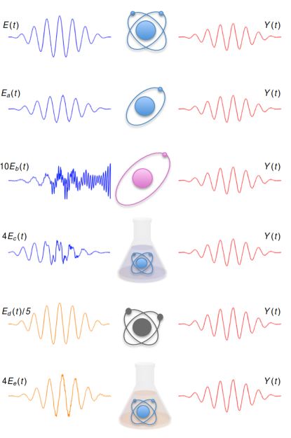
Figure 1: The control fields $E_{a}(t)$, $E_{b}(t)$, $E_{c}(t)$, $E_{d}(t)$ and $E_{e}(t)$ induce the same nonlinear optical response $Y(t)$ on: closed quantum systems (a) and (b), (c) an open quantum system, (d) an closed classical system and (e) an open classical system. In (a) and (b), the system is a hydrogen atom initially prepared in the ground and first excited states, respectively. $E_{b}(t)$, $E_{d}(t)$ and $E_{e}(t)$ are scaled for comparison with the first field $E(t)$ that is applied to a model of an argon atom to produce the induced dipolar spectra $Y(t)$ ,which is used for tracking in the remaining cases. Compare with Fig. 2 (f) for the importance of small differences in the control fields, which are not apparent in the time domain.

Summary of results. We want the induced dipole spectra (IDS) of an $N$-electron system, $\vec{y}(t)=\sum_{k=1}^{N}\langle\vec{\hat{\boldsymbol{x}}}_{k}\rangle$, to follow (i.e., track) a predefined time-dependent vector $\vec{Y}(t)$; atomic units (a.u.) with $\hbar=m=e=1$ are used throughout. In particular, assuming that $\vec{y}(t)=\vec{Y}(t)$ at some time moment $t$, then the control field $\vec{E}(t+dt)$ enforcing $\vec{y}(t+dt)=\vec{Y}(t+dt)$ at the next time step $t+dt$ is given by

$$\vec{E}(t+dt)=-\frac{4}{Ndt}\left[\left\langle\sum_{k=1}^{N}\vec{\hat{\boldsymbol{p}}}_{k}\right\rangle-\frac{\vec{Y}(t+dt)-\vec{Y}(t)}{dt}\right]$$

$$\quad+\frac{2}{N}\left\langle\sum_{k=1}^{N}\mathbf{\nabla}_{k}V_{k}(\vec{\hat{\boldsymbol{x}}}_{k})\right\rangle-\frac{2}{N}\left\langle\sum_{k=1}^{N}\vec{A}_{k}\right\rangle-\vec{E}(t)+O\left(dt\right),$$ (1)

where $dt$ is an infinitesimal time increment, $\left\langle-\nabla_{k}V(\vec{\hat{\boldsymbol{x}}}_{k})\right\rangle(t)$ and $\langle\vec{A}_{k}\rangle(t)$ describe the interaction with a potential force and an environment, respectively (see Sec. I of Supplemental Material Sup for details, which includes Ref. Bandrauk and Shen (1992)). The state (i.e., the density matrix and the probability distribution in the quantum and classical cases, respectively) determining the expectation values is propagated to the next time moment via the corresponding equation of motion (see, e.g., Table 1) using $\vec{E}(t+dt)$. Having calculated $\vec{E}(t)$ for all times, the dynamical equation is used to verify satisfaction of the tracking condition $\vec{y}(t)=\vec{Y}(t)$.

Since Eq. (1) has exactly the same structure of the single particle case, we will study systems with single-electron excitation (i.e., $N=1$) in one spatial dimension. In this case, Eq. (1) takes the form

$$E(t+dt)= -\frac{4}{dt}\left[\left\langle\hat{\boldsymbol{p}}\right\rangle(t)-\frac{Y(t+dt)-Y(t)}{dt}\right]$$

$$+2\left\langle V^{\prime}(\hat{\boldsymbol{x}})\right\rangle(t)-2\langle A\rangle(t)-E(t)+O\left(dt\right),$$ (2)

where $\left\langle-V^{\prime}(\hat{\boldsymbol{x}})\right\rangle$ and $\langle A\rangle$ are specified in Table 1 for widely used models. The described scheme constitutes SDM, as the distinct physical systems in Fig. 1 produced the same $Y(t)$, yet the resulting control fields calculated from Eq. (2) are unique once the system’s initial state is supplied.

The physical meaning of Eq. (2) is that a desired polarizability can be induced from any dynamical system as long as no constraints are imposed on the driving laser field. In this fashion, the IDS of any two atomic or molecular systems can be made identical by applying the specific required pulse shapes.

Type of system	$\langle O\rangle$	$\langle A\rangle(t)$	Equations of motion
Closed Quantum	${\rm Tr}\,[\hat{\rho}\hat{O}]$	$0$	$i\hbar d\hat{\rho}/dt=[\hat{H},\hat{\rho}]$
Open Quantum	${\rm Tr}\,[\hat{\rho}\hat{O}]$	$-2\gamma\langle\hat{\boldsymbol{p}}\rangle$	Caldeira-Legget equation, Eq. (5)
Closed Classical	$\frac{1}{N}\sum_{i=1}^{N}O(x_{i}(t),p_{i}(t))$	$0$	Newton’s equations, Eq. (6)
Open Classical	$\int dxdpO(x,p)\rho(x,p,t)$	$-2\gamma\langle p\rangle$	Fokker-Planck equation, Eq. (8)

Table 1: The dynamical systems, averages and equations of motions analyzed in this Letter. In all quantum cases, we have $\hat{H}=\hat{H}_{0}-\hat{\boldsymbol{x}}E(t)$, where $\hat{H}_{0}=\hat{\boldsymbol{p}}^{2}/2+V(\hat{\boldsymbol{x}})$. The atoms are represented as a single active electron moving in the field of a soft-Coulomb potential $V(x)=-Z_{e}/\sqrt{x^{2}+a^{2}}$, where $Z_{e}$ is the effective charge of the atom and both $Z_{e}$ and $a$ are chosen such that the experimental value of the ionization potential is reproduced. In the open classical case, $\rho(x,p,t)$ correspond to the particle’s probability density in the phase space.

Such versatility of SDM is due to the fact that the induced dynamics takes advantage of the continuum. The IDS $y(t)$, as an expectation value of $\hat{\boldsymbol{x}}$, can attain arbitrary values only if the coordinate $\hat{\boldsymbol{x}}$ is unrestricted. Moreover, if a strong field $E(t)$ is required to match an IDS, then $E(t)$ may induce ionization necessitating the coupling to the continuum. Mathematically, this means that $\hat{\boldsymbol{x}}$ and $\hat{\boldsymbol{p}}$ need to act in an infinite dimensional Hilbert space.

Equation (2) is a special case of tracking control Gross et al. (1993): Given a desired target $Z(t)$, find the control $E(t)$ such that $Z(t)=z(t)$ with $z(t)=\langle\hat{O}\rangle$ for a chosen observable $\hat{O}$. For simplicity, consider a closed quantum system ($\hat{A}=0$) with the hamiltonian $\hat{H}(t)=\hat{H}_{0}-E(t)\hat{\mu}$ and $[\hat{O},\hat{\mu}]=0$. The corresponding Ehrenfest theorem then reads

$$\frac{d^{2}Z(t)}{dt^{2}}=-\left\langle[\hat{H}_{0},[\hat{H}_{0},\hat{O}]]\right\rangle+\left\langle[\hat{\mu},[\hat{H}_{0},\hat{O}]]\right\rangle E(t).$$ (3)

Given $Z(t)$, Eq. (3) is solved with respect to the unknown $E(t)$. Tracking control has been typically applied to finite-level quantum systems. In this case, $\langle[\hat{\mu},[\hat{H}_{0},\hat{O}]]\rangle$ may vanish at some time $t$, leading to a singularity in $E(t)$. There is no general way to prevent these singularities in finite dimensional tracking irrespective of the form of the finite dimensional matrices $\hat{H}_{0}$, $\hat{\mu}$, and $\hat{O}$ . Note that SDM is free of such singularities by construction .

According to Eq. (2), the control field is shaped in time domain, thus possibly introducing high frequency components beyond the target response bandwidth $\omega/\omega_{0}\gtrsim 23$, as seen in Fig. 2. However, those high frequencies are not important for the dynamics, since removing all frequencies outside the target response bandwidth, (i.e., for $\omega/\omega_{0}\gtrsim 23$) in the tracking fields $E_{a}(t)$, $E_{c}(t)$ and $E_{d}(t)$, does not significantly affect the tracking condition $y(t)=Y(t)$. Moreover, SDM is robust to the presence of multiplicative noise in the tracking (see Sec. II of Supplemental Material Sup for details, which includes Ref. Bandrauk and Shen (1992)).

Equation (2) describes a broad variety of dynamical systems (Table 1). As illustrations, we apply SDM to the following models: (a) and (b) closed quantum systems governed by the von Neumann equation, (c) open quantum systems modeled by the Caldeira-Legget master equation Caldeira and Leggett (1983a, b), (d) classical closed systems obeying Newton’s equations, and (e) open classical systems described by the Fokker-Planck equation Gardiner et al. (1985). In all these cases, we track the target $Y(t)$, which is obtained as an IDS of an isolated argon atom treated as having one electron responding to a band limited field $E(t)=0.04\cos(\omega_{0}t)f(t)$ of central frequency $\omega_{0}=0.06$ (a.u) (756 nm) and the envelope $f(t)=\cos^{2}(\pi t/(2t_{f}))$, where the final propagation time is $t_{f}=8\pi/\omega_{0}$. Figure 2 depicts the spectrum of $Y(t)$ exhibiting high harmonic generation (HHG) Corkum (1993); Winterfeldt et al. (2008).

We employ the single active electron approach Bauer (1997) to model atomic systems throughout. Hence, an atom is represented by a single particle moving in the field of a soft-Coulomb potential

$$V(x)=\frac{-Z_{e}}{\sqrt{x^{2}+a^{2}}},$$ (4)

where the effective charge $Z_{e}\approx 1$ and radius $a$ is adjusted such that the ground state energy in each case matches the experimental ionization potential. For example, $Z_{e}=1$ and $a^{2}=2$ (a.u.) models a hydrogen atom, while $Z_{e}=1$ and $a^{2}=1.37$ (a.u.) are used for argon. Since there is no degeneracy in the spectrum of one dimensional quantum systems, the eigenstates are labelled only by the principal quantum number $n$.

Making two closed quantum systems look alike. As a first example of SDM, we make hydrogen ‘look like’ argon by matching their IDS. We find the shape of the laser field $E_{a}(t)$ [Eq. (2)] that induces an optical response $Y(t)$ in a hydrogen atom initially in the ground state ($n=1$), modeled as a closed quantum system. Superimposing the Fourier transforms of $E_{a}(t)$ and $Y(t)$ in Fig. 2 (a), we note that the tracking field bandwidth is broader than the target bandwidth. This trend is observed in all examples presented in this Letter. Moreover, the third harmonic ($3\omega_{0}$) in the tracking field is an order of magnitude smaller than the same frequency in $Y(t)$. A further analysis reveals that the induced response is at best weakly dependent of the third harmonic in the driving field. Thus, the $3\omega_{0}$ generation in hydrogen occurs via parametric down conversion Boyd (2008).

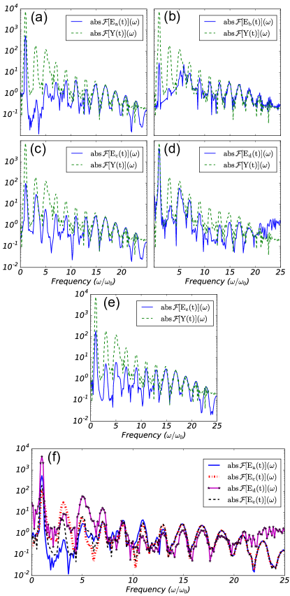
Figure 2: (color online) The control fields $E_{a}(t)$, $E_{b}(t)$, $E_{c}(t)$, $E_{d}(t)$, $E_{e}(t)$ and the target IDS $Y(t)$ from Fig. 1 in frequency domain. $\rm abs\,\mathcal{F}[\cdot]$ denotes the absolute value of the Fourier transform. The $\omega_{0}$ is the carrier frequency of $E(t)$ in Fig. 1.

As mentioned earlier, the control fields calculated using SDM are unique once the system’s initial state is specified. For the control field $E_{a}(t)$ shown in Fig. 1, the hydrogen atom was initially in the ground state; however, a very different control field is required ($E_{b}(t)$ in Figs. 1 and 2 (b)) if the hydrogen atom is initially in the first excited state ($n=2$). The amplitude of $E_{b}(t)$ is nearly a factor of ten smaller than $E_{a}(t)$ (see Fig. 1) since the energy gap between the ground and first excited states in the hydrogen atom is approximately half the ionization potential. Moreover, for the hydrogen atom in the first excited state, single photon ionization takes place for $\omega/\omega_{0}\approx 5$, whereas parametric down conversion dominates the dynamics for $\omega/\omega_{0}\lesssim 7$ (see Fig. 2 (b)). For higher frequencies where $\omega/\omega_{0}\gtrsim 7$, linear response takes place.

Making open and closed quantum systems look alike. The effects of energy damping and dephasing are commonly modeled by the Caldeira-Legget master equation Caldeira and Leggett (1983a, b)

$$i\frac{d\hat{\rho}}{dt}=[\hat{H},\hat{\rho}]+i\mathcal{L}[\hat{\rho}],\quad\mathcal{L}[\hat{\rho}]=-i\gamma[\hat{\boldsymbol{x}},[\hat{\boldsymbol{p}},\hat{\rho}]]-\chi[\hat{\boldsymbol{x}},[\hat{\boldsymbol{x}},\hat{\rho}]],$$ (5)

where $\chi=2\gamma kT$. Using Eq. (2) with the damping term $\langle A\rangle=-2\gamma\langle\hat{\boldsymbol{p}}\rangle$ as specified in Table 1, we find the control field $E_{c}(t)$ (Fig. 2 (c)) that induces the optical response of the atomic argon, interacting with a dissipative environment, to match the nonlinear spectra of the isolated argon $Y(t)$ shown in Fig. 1. The amplitude damping time and temperature were chosen as $\gamma^{-1}\approx$ 242 fs and $T\approx$ 100 K, correspondingly.

According to dynamical decoupling Viola and Lloyd (1998); Facchi et al. (2005); Ban (1998); Cappellaro et al. (2006), appropriately designed laser pulses can compensate for the interaction of a quantum system with the environment. Dynamical decoupling usually relies on a perturbative treatment of the environment; whereas, SDM [Eq. (2)] is explicitly nonperturbative in both the field and environmental interactions.

HHG is an important source for creating attosecond pulses. A weak HHG signal is often obtained by irradiating a low pressure inert gas with a band limited pulse Winterfeldt et al. (2008). The intensity of HHG is proportional to the gas concentration. However, the denser the gas, the less isolated the atomic system becomes, giving rise to decoherent dynamics, thus suppressing HHG Constant et al. (1999). The presented SDM illustration shows that the HHG spectra of an isolated system can be reproduced even from an open system by properly pulse shaping the incident laser field.

Making closed classical and quantum systems look alike. The position and momentum of an ensemble of $N$ classical particles obey Newton’s equations

$$\frac{d}{dt}x_{i}(t)=p_{i}(t),\quad\frac{d}{dt}p_{i}(t)=-V^{\prime}(x_{i}(t))+E(t),$$ (6)

where $V(x)$ is given by Eq. (4). The ensemble’s initial momentum and positions are randomly generated by the normal distribution with zero mean and standard deviation of $1$. According to Table 1, the IDS of the classical system $y_{d}(t)$ is given by $y_{d}(t)=\frac{1}{N}\sum_{i=1}^{N}\,x_{i}(t).$ From Eq. (2), we find the control field $E_{d}(t)$ (Fig. 2 (d)) that forces the IDS of the classical argon model [Eq. (6)] to match the IDS of the isolated argon $Y(t)$.

The dynamics underlying the classical IDS $y(t)$ induces nonlinear optical processes. In particular, the further the trajectory goes from the center of force (i.e., the origin), the more harmonics it yields. This can be seen from the following taylor expansion of Eq. (6)

$$\frac{d}{dt}p_{i}(t)\approx E(t)-\frac{Z_{e}}{a^{3}}x_{i}(t)+\frac{3Z_{e}}{2a^{5}}x_{i}(t)^{3}+O\left(x_{i}(t)^{5}\right).$$ (7)

The first two terms on the right hand side correspond to a driven harmonic oscillator. Therefore, the trajectories closest to the origin only linearly respond to the control field $E(t)$; whereas, the trajectories farther away give rise to high harmonics. As can be seen in Fig. 2 (f), the spectrum of the classical control field $E_{d}(t)$ deviates significantly from the previously obtained control fields $E_{a}(t)$, $E_{c}(t)$ and $E_{e}(t)$ for the quantum cases. As in system (a) of Figs. 1 and 2 (a), suppressing the third harmonic ($3\omega_{0}$) in the classical control field does not significantly affect the response. It is noteworthy that significantly nonlinear classical dynamics can be indistinguishable from quantum evolution Franco et al. (2010); Schwieters and Rabitz (1993); Blackburn et al. (2016).

Making open classical and closed quantum systems look alike. The state of an open classical system can be specified by a positive probability distribution function $\rho=\rho(x,p,t)$ defined on a classical phase space. The dynamics of such a system is commonly modeled by the Fokker-Planck equation Gardiner et al. (1985)

$$\frac{\partial\rho}{\partial t}=\left[-\frac{\partial}{\partial x}p+(V^{\prime}(x)-E(t))\frac{\partial}{\partial p}+2\gamma\frac{\partial}{\partial p}p+D\frac{\partial^{2}}{\partial p^{2}}\right]\rho,$$ (8)

where $D=0.01$ (a.u.) denotes a diffusion coefficient and $\gamma=0.001$ (a.u.) quantifies energy damping.

Following Ref. Cabrera et al. (2015), we use Eq. (8) as a classical counterpart of the Caldeira-Legget Eq. (5), modeling the atomic argon interacting with a dissipative bath. From Eq. (2) with $\langle A\rangle=-2\gamma\langle p\rangle$ as specified in Table 1, we find the control field $E_{e}(t)$ (Figs. 1 and 2 (e)) that forces the IDS of the argon classical model [Eq. (8)] to match the IDS of the isolated argon $Y(t)$.

It is important to note the remarkable similarity between $E(t)$ and $E_{e}(t)$ in Fig. 1. In fact, for our particular example of open classical dynamics, the intensity of the IDS is proportional to the intensity of the control field $E_{e}(t)$. Furthermore, reducing the intensity of any individual frequency in the control field linearly decreases the intensity of the corresponding harmonic in the IDS without influencing the other frequencies. This shows that there is only a linear optical process taking place. Moreover, there are no cooperative effects between different frequency components – a consequence of strong decoherence in the particular example of open classical dynamics considered here (see also Ref. Franco et al. (2010)).

The spectrum of the tracking fields $E_{a}(t)$, $E_{c}(t)$, $E_{d}(t)$ and $E_{e}(t)$ are shown in Fig. 2 (f). Subsequent analysis indicates that the optical responses for the closed (a) and open (c) quantum systems are nonlinear in the frequency ranges of $\omega/\omega_{0}\lesssim 13$ and $\omega/\omega_{0}\lesssim 7$, respectively. Similar to our simulations of the open classical system (e), laser-matter interactions described within the classical and quantum electrodynamics coincide in the linear response regime Andrews and Bradshaw (2004); Duque et al. (2015). In contrast, the closed classical system (d) displays strong nonlinear effects overall, as can be seen in Fig. 2 (d) and (f).

Conclusions. We put forward the paradigm of SDM in which laser fields are shaped to make any distinct dynamical system look identical spectrally to any other system. As a result, the observed IDS without any information on the driving field cannot be used to unambiguously characterize atomic and molecular systems.

SDM can be applied to many important problems. For example, it can be seen as the opposite of Optimal Dynamic Discrimination (ODD) which shows that nearly identical quantum systems may be distinguished by means of their dynamics induced by properly shaped laser pulses Li et al. (2002); Goun et al. (2016). ODD has been experimentally confirmed for a number of nominally similar systems Brixner et al. (2001); Tkaczyk et al. (2008); Roth et al. (2009); Petersen et al. (2010); Rondi et al. (2011, 2012). In future works, we plan to reformulate ODD as a tracking control problem (in the spirt of SDM) in order to propose novel methods for the concentration characterization of a mixture of complex molecular species with similar linear spectra. This problem is inspired by the challenges in the life sciences Constant et al. (1999); Feng et al. (2000); Bagwell and Adams (1993); Speicher et al. (1996); Perfetto et al. (2004). ODD may also be used to find control fields that optimally discriminate between classical and quantum models of the same physical system, thereby shading light on ongoing discussions Schwieters and Rabitz (1993); Blackburn et al. (2016); Franco et al. (2010). Moreover, being non-perturbative in both the control field and environment interactions, SDM offers a potential alternative to dynamical decoupling Viola and Lloyd (1998); Facchi et al. (2005); Ban (1998); Cappellaro et al. (2006). Furthermore, in the framework of SDM, HHG spectra of an isolated system can be induced from an open system by pulse shaping the incident laser field, providing an efficient way to generate bright HHG from dense atomic gases. In addition, the high degree of robustness to noise of the tracking fields (see Sec. II of Supplemental Material Sup , which includes Ref. Bandrauk and Shen (1992)) makes SDM suited for experimental applications.

As a final remark, a recently experiment Sommer et al. (2016) demonstrated the feasibility of simultaneous characterization of the control field as well as IDS, opening a possibility of SDM experimental realization.

Acknowledgments. A.G.C. acknowledges financial support from NSF CHE 1464569, D.I.B. from DOE DE-FG02-02-ER-15344, R.C. from ARO W911NF-16-1-0014 and H.R. from DARPA W911NF-16-1-0062. A.G.C. was also supported by the Fulbright foundation. D.I.B. is also supported by 2016 AFOSR Young Investigator Research Program. We would like to acknowledge an anonymous referee for drawing our attention to Ref. Blackburn et al. (2016).

A.G.C. and D.I.B. contributed equally to this work.

Supplemental Material for: “Making Distinct Dynamical Systems Appear Spectrally Identical”

I Derivation of Equation (1) from the main text

Consider open system dynamics, with Hamiltonian for $N$ interacting particles having the form

$$\hat{H}(t) =\sum_{k=1}^{N}\frac{\hat{\boldsymbol{p}}^{2}_{k}}{2}+\sum_{k=1}^{N}V_{i}(\vec{\hat{\boldsymbol{x}}}_{k})-\sum_{k=1}^{N}\vec{\hat{\boldsymbol{x}}}_{k}\cdot\vec{E}(t)+\frac{1}{2}\sum_{k,j=1}^{N}U(|\vec{\hat{\boldsymbol{x}}}_{k}-\vec{\hat{\boldsymbol{x}}}_{j}|),$$ (9)

where $V_{i}(\vec{\hat{\boldsymbol{x}}}_{k})$ corresponds to the interaction between each particle of the system and an external potential, $U(|\vec{\hat{\boldsymbol{x}}}_{k}-\vec{\hat{\boldsymbol{x}}}_{j}|)$ describes the inter-particle interaction and $\vec{E}(t)$ is the applied laser field. The dynamical equation for the open system dynamics with the above Hamiltonian is

$$\frac{d}{dt}\hat{\rho}(t)=\mathcal{L}[\hat{\rho}(t)],$$ (10)

with

$$\mathcal{L}[\odot]=-i[\hat{H}(t),\odot]+\mathcal{D}[\odot],$$ (11)

where $\mathcal{D}[\hat{\rho}(t)]$ describes the coupling between the system and the environment. The time evolution of the density matrix from the instant $t$ to the next instant $t+dt$ in the super-operator formalism is

$$\hat{\rho}(t+dt)=\mathcal{T}e^{\int_{t}^{t+dt}\mathcal{L}[\odot]d\tau}\hat{\rho}(t),$$ (12)

where $dt$ is an infinitesimal time increment and $\mathcal{T}$ is the time-ordering operator.

Given $\vec{Y}(t)=\sum_{k=1}^{N}\left\langle\vec{\hat{\boldsymbol{x}}}_{k}\right\rangle(t)$ at time $t$ , we would like to find the control field $E(t+dt)$ such that

$$\vec{Y}(t+dt) =\sum_{k=1}^{N}\left\langle\vec{\hat{\boldsymbol{x}}}_{k}\right\rangle(t+dt)$$

$$=\sum_{k=1}^{N}{\rm Tr}\left[\vec{\hat{\boldsymbol{x}}}_{k}\hat{\rho}(t+dt)\right]=\sum_{k=1}^{N}{\rm Tr}\left[\vec{\hat{\boldsymbol{x}}}_{k}\,\mathcal{T}e^{\int_{t}^{t+dt}\mathcal{L}[\odot]d\tau}\hat{\rho}(t)\right]$$

$$=\sum_{k=1}^{N}{\rm Tr}\left[\vec{\hat{\boldsymbol{x}}}_{k}e^{\int_{t}^{t+dt}\mathcal{L}[\odot]d\tau}\hat{\rho}(t)\right]+O\left(dt^{3}\right)$$

$$=\sum_{k=1}^{N}{\rm Tr}\left[\vec{\hat{\boldsymbol{x}}}_{k}e^{dt\mathcal{L}_{D}[\odot]}\hat{\rho}(t)\right]+O\left(dt^{3}\right)$$

$$=\sum_{k=1}^{N}\left\langle\vec{\hat{\boldsymbol{x}}}_{k}\right\rangle(t)+\sum_{k=1}^{N}\ {\rm Tr}\left[\vec{\hat{\boldsymbol{x}}}_{k}\left(dt\mathcal{L}_{D}[\hat{\rho}(t)]+\frac{dt^{2}}{2}\mathcal{L}_{D}[\mathcal{L}_{D}[\hat{\rho}(t)]]\right)\right]+O\left(dt^{3}\right)$$

$$=\sum_{k=1}^{N}\left\langle\vec{\hat{\boldsymbol{x}}}_{k}\right\rangle(t)+\sum_{k=1}^{N}\ {\rm Tr}\left[\left(dt\mathcal{L}_{D}^{\dagger}[\vec{\hat{\boldsymbol{x}}}_{k}]+\frac{dt^{2}}{2}\mathcal{L}_{D}^{\dagger}[\mathcal{L}_{D}^{\dagger}[\vec{\hat{\boldsymbol{x}}}_{k}]]\right)\hat{\rho}(t)\right]+O\left(dt^{3}\right)$$

where

$$\mathcal{L}_{D}[\odot]=-\frac{i}{2}[\hat{H}(t+dt)+\hat{H}(t),\odot]+\mathcal{D}[\odot],$$ (14)

and the factor of $2$ comes from using the midpoint rule to approximate the integral over time (see, e.g., Ref. Bandrauk and Shen (1992)). We also used the following definition of the adjoint

$${\rm Tr}\left[\hat{\vec{\boldsymbol{x}}}_{k}\mathcal{L}_{D}\left[\hat{\rho}(t)\right]\right]={\rm Tr}\left[\mathcal{L}_{D}^{\dagger}\left[\hat{\vec{\boldsymbol{x}}}_{k}\right]\hat{\rho}(t)\right],$$ (15)

where

$$\mathcal{L}_{D}^{\dagger}[\vec{\hat{\boldsymbol{x}}}_{k}]=\frac{i}{2}[\hat{H}(t+dt)+\hat{H}(t),\vec{\hat{\boldsymbol{x}}}_{k}]+\mathcal{D}^{\dagger}[\vec{\hat{\boldsymbol{x}}}_{k}].$$ (16)

Let us assume that $\mathcal{D}^{\dagger}[\vec{\hat{\boldsymbol{x}}}_{k}]=0$, since all examples studied in the main text have this property. In this case, we have

$$\mathcal{L}_{D}^{\dagger}[\mathcal{L}_{D}^{\dagger}[\vec{\hat{\boldsymbol{x}}}_{k}]]=\frac{i}{2}[\hat{H}(t+dt)+\hat{H}(t),\vec{\hat{\boldsymbol{p}}}_{k}]+\mathcal{D}^{\dagger}[\vec{\hat{\boldsymbol{p}}}_{k}]=-\vec{\nabla}_{k}V_{k}(\vec{\hat{\boldsymbol{x}}}_{k})+\frac{1}{2}(\vec{E}(t+dt)+\vec{E}(t))+\mathcal{D}^{\dagger}[\vec{\hat{\boldsymbol{p}}}_{k}],$$ (17)

since $-\sum_{k,j=1}^{N}\vec{\nabla}_{k}U(|\vec{\hat{\boldsymbol{x}}}_{k}-\vec{\hat{\boldsymbol{x}}}_{j}|)=\sum_{k,j=1}^{N}\vec{F}_{kj}=0$ due to Newton’s third law, $\vec{F}_{jk}=-\vec{F}_{kj}$.

Thus, finally

$$\vec{E}(t+dt)=-\frac{4}{Ndt}\left[\sum_{i=1}^{N}\left\langle\vec{\hat{\boldsymbol{p}}}_{i}\right\rangle(t)-\frac{\vec{Y}(t+dt)-\vec{Y}(t)}{dt}\right]+\frac{2}{N}\sum_{i=1}^{N}\left\langle\vec{\nabla}_{i}V_{i}(\vec{\hat{\boldsymbol{x}}}_{i})\right\rangle(t)-\frac{2}{N}\sum_{k=1}^{N}\langle\vec{\hat{A}}_{k}\rangle-\vec{E}(t)+O\left(dt\right),$$ (18)

where $\vec{\hat{A}}_{k}=\mathcal{D}^{\dagger}\left[\vec{\hat{\boldsymbol{p}}}_{k}\right]$. Performing a Taylor expansion in $\vec{Y}(t+dt)$, we get an equivalent result

$$\vec{E}(t+dt)=-\frac{4}{Ndt}\left[\sum_{i=1}^{N}\left\langle\vec{\hat{\boldsymbol{p}}}_{i}\right\rangle(t)-\vec{Y^{\prime}}(t)\right]+\frac{2}{N}\vec{Y^{\prime\prime}}(t)+\frac{2}{N}\sum_{i=1}^{N}\left\langle\vec{\nabla}_{i}V_{i}(\vec{\hat{\boldsymbol{x}}}_{i})\right\rangle(t)-\frac{2}{N}\sum_{k=1}^{N}\langle\vec{\hat{A}}_{k}\rangle-\vec{E}(t)+O\left(dt\right),$$ (19)

which makes the connection with the Ehrenfest theorems explicit.

II Robustness to noise

There are many different types of noise in lasers including phase, intensity and frequency noise. In order to assess the robustness of SDM, we consider the laser field $E_{a,b,c}(t)$ to be contaminated by a multiplicative noise. The model for the noisy laser field is

$$\bar{E}_{a,b,c}(t)=E_{a,b,c}(t)\left(1+W[0,\sigma_{a,b,c},t]\right),$$ (20)

where $W[\mu,\sigma,t]$ is a normally distributed random variable with the mean $\mu=0$ and standard deviation $\sigma_{a,b}=0.02$ and $\sigma_{c}=0.05$, subscripts (a) and (b) denote closed and (c) open quantum systems ( see Fig. 1 in the main text). The signal to noise ratio of the field’s amplitude is

$$SNR_{a,b,c}=\frac{\langle\bar{E}_{a,b,c}(t)\rangle}{\sqrt{Var[\bar{E}_{a,b,c}(t)]}}=\frac{1}{\sigma_{a,b,c}}.$$ (21)

The relative distance between the noise-free target IDS $Y(t)$ and the system’s IDS $y(t)$ induced by the contaminated control field [Eq. (20] is estimated as

$$d(y(t),Y(t))^{2}=\frac{\int dt|y(t)-Y(t)|^{2}}{\int dt|Y(t)|^{2}}.$$ (22)

Quantity (22) evaluated for different noise realizations is shown in Figs. 3 and 4 for the closed and open quantum system, respectively. In the open quantum system case, we observe that the values of the relative distance (22) calculated with noise fluctuate around the noise-free value. On the other hand, in Fig. 3 we note that the average value of the relative distance (22) generated by the noisy control fields (blue solid line) is approximately $18\%$ larger than the corresponding values for the noise-free tracking field (red dashed line).

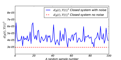
Figure 3: (color online) Plot of $d(y(t),Y(t))^{2}$ for the response generated by the closed system’s control field with noise (solid blue line) and without noise (red dashed line).

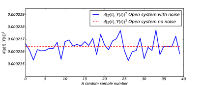
Figure 4: (color online) Plot of $d(y(t),Y(t))^{2}$ for the response generated by the open system’s control field with noise (solid blue line) and without noise (red dashed line).

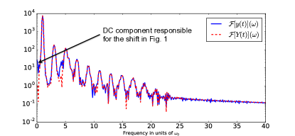
Figure 5: (color online) Plot of $\mathcal{F}[y(t)](\omega)$ for the closed system’s IDS generated by the noisy field (blue, full curve) and the target IDS $\mathcal{F}[Y(t)](\omega)$ (red, dotted line). For this particular example, $d(y(t),Y(t))^{2}=6.5\times 10^{-5}$.

For the closed quantum systems, the noisy control field generates a DC component in the IDS (see Fig. 5 bellow), shifting the average relative distance.

References

- Gust et al. (2001) D. Gust, T. A. Moore, and A. L. Moore, Accounts of Chemical Research 34, 40 (2001).
- Cremer et al. (2002) S. Cremer, M. F. Sledge, and J. Heinze, Nature 419, 897 (2002).
- van Kasteren et al. (2007) S. I. van Kasteren, H. B. Kramer, H. H. Jensen, S. J. Campbell, J. Kirkpatrick, N. J. Oldham, D. C. Anthony, and B. G. Davis, Nature 446, 1105 (2007).
- Leininger et al. (2000) S. Leininger, B. Olenyuk, and P. J. Stang, Chemical Reviews 100, 853 (2000).
- Zhang et al. (2005) Z. Zhang, A. S. Keys, T. Chen, and S. C. Glotzer, Langmuir 21, 11547 (2005).
- Mitov et al. (2002) M. Mitov, C. Portet, C. Bourgerette, E. Snoeck, and M. Verelst, Nature materials 1, 229 (2002).
- Whitesell et al. (1994) J. K. Whitesell, R. E. Davis, M. S. Wong, and N. L. Chang, Journal of the American Chemical Society 116, 523 (1994).
- Chirik and Wieghardt (2010) P. Chirik and K. Wieghardt, Science 327, 794 (2010).
- Gust et al. (1993) D. Gust, T. A. Moore, and A. L. Moore, Accounts of Chemical Research 26, 198 (1993).
- De Silva et al. (1997) A. P. De Silva, H. N. Gunaratne, T. Gunnlaugsson, A. J. Huxley, C. P. McCoy, J. T. Rademacher, and T. E. Rice, Chemical Reviews 97, 1515 (1997).
- Della Gaspera et al. (2014) E. Della Gaspera, J. van Embden, A. S. Chesman, N. W. Duffy, and J. J. Jasieniak, ACS applied materials & interfaces 6, 22519 (2014).
- Rabong et al. (2014) C. Rabong, C. Schuster, T. Liptaj, N. Prónayová, V. B. Delchev, U. Jordis, and J. Phopase, RSC Advances 4, 21351 (2014).
- (13) See Supplemental Material at ***************************.
- Bandrauk and Shen (1992) A. D. Bandrauk and H. Shen, Canadian Journal of Chemistry 70, 555 (1992).
- Gross et al. (1993) P. Gross, H. Singh, H. Rabitz, K. Mease, and G. Huang, Physical Review A 47, 4593 (1993).
- Caldeira and Leggett (1983a) A. O. Caldeira and A. J. Leggett, Physica A: Statistical mechanics and its Applications 121, 587 (1983a).
- Caldeira and Leggett (1983b) A. Caldeira and A. J. Leggett, Annals of Physics 149, 374 (1983b).
- Gardiner et al. (1985) C. W. Gardiner et al., Handbook of stochastic methods, vol. 4 (Springer Berlin, 1985).
- Corkum (1993) P. B. Corkum, Phys. Rev. Lett. 71 (1993).
- Winterfeldt et al. (2008) C. Winterfeldt, C. Spielmann, and G. Gerber, Rev. Mod. Phys. 80 (2008).
- Bauer (1997) D. Bauer, Phys. Rev. A 56 (1997).
- Boyd (2008) R. W. Boyd, Nonlinear Optics, Third Edition (Academic Press, 2008).
- Viola and Lloyd (1998) L. Viola and S. Lloyd, Phys. Rev. A 58 (1998).
- Facchi et al. (2005) P. Facchi, S. Tasaki, S. Pascazio, H. Nakazato, A. Tokuse, and D. A. Lidar, Phys. Rev. A 71 (2005).
- Ban (1998) M. Ban, journal of modern optics 45, 2315 (1998).
- Cappellaro et al. (2006) P. Cappellaro, J. Hodges, T. Havel, and D. Cory, The Journal of chemical physics 125, 044514 (2006).
- Constant et al. (1999) E. Constant, D. Garzella, P. Breger, E. Mével, C. Dorrer, C. Le Blanc, F. Salin, and P. Agostini, Phys. Rev. Lett. 82, 1668 (1999).
- Franco et al. (2010) I. Franco, M. Spanner, and P. Brumer, Chemical Physics 370, 143 (2010).
- Schwieters and Rabitz (1993) C. D. Schwieters and H. Rabitz, Physical Review A 48, 2549 (1993).
- Blackburn et al. (2016) J. A. Blackburn, M. Cirillo, and N. Grønbech-Jensen, Physics Reports 611, 1 (2016).
- Cabrera et al. (2015) R. Cabrera, D. I. Bondar, K. Jacobs, and H. A. Rabitz, Phys. Rev. A 92, 042122 (2015).
- Andrews and Bradshaw (2004) D. L. Andrews and D. S. Bradshaw, European journal of physics 25, 845 (2004).
- Duque et al. (2015) S. Duque, P. Brumer, and L. A. Pachón, Phys. Rev. Lett. 115, 110402 (2015).
- Li et al. (2002) B. Li, G. Turinici, V. Ramakrishna, and H. Rabitz, The Journal of Physical Chemistry B 106, 8125 (2002).
- Goun et al. (2016) A. Goun, D. I. Bondar, O. E. Ali, Z. Quine, and H. A. Rabitz, Scientific reports 6, 25827 (2016).
- Brixner et al. (2001) T. Brixner, N. Damrauer, P. Niklaus, and G. Gerber, Nature 414, 57 (2001).
- Tkaczyk et al. (2008) E. R. Tkaczyk, K. Mauring, A. H. Tkaczyk, V. Krasnenko, J. Y. Ye, J. R. Baker, and T. B. Norris, Biochemical and biophysical research communications 376, 733 (2008).
- Roth et al. (2009) M. Roth, L. Guyon, J. Roslund, V. Boutou, F. Courvoisier, J.-P. Wolf, and H. Rabitz, Physical review letters 102, 253001 (2009).
- Petersen et al. (2010) J. Petersen, R. Mitrić, V. Bonačić-Kouteckỳ, J.-P. Wolf, J. Roslund, and H. Rabitz, Physical review letters 105, 073003 (2010).
- Rondi et al. (2011) A. Rondi, D. Kiselev, S. Machado, J. Extermann, S. Weber, L. Bonacina, J.-P. Wolf, J. Roslund, M. Roth, and H. Rabitz, CHIMIA International Journal for Chemistry 65, 346 (2011).
- Rondi et al. (2012) A. Rondi, L. Bonacina, A. Trisorio, C. Hauri, and J.-P. Wolf, Physical Chemistry Chemical Physics 14, 9317 (2012).
- Feng et al. (2000) G. Feng, R. H. Mellor, M. Bernstein, C. Keller-Peck, Q. T. Nguyen, M. Wallace, J. M. Nerbonne, J. W. Lichtman, and J. R. Sanes, Neuron 28, 41 (2000).
- Bagwell and Adams (1993) C. B. Bagwell and E. G. Adams, Annals of the New York Academy of Sciences 677, 167 (1993).
- Speicher et al. (1996) M. R. Speicher, S. G. Ballard, and D. C. Ward, Nature genetics 12, 368 (1996).
- Perfetto et al. (2004) S. P. Perfetto, P. K. Chattopadhyay, and M. Roederer, Nature Reviews Immunology 4, 648 (2004).
- Sommer et al. (2016) A. Sommer, E. Bothschafter, S. Sato, C. Jakubeit, T. Latka, O. Razskazovskaya, H. Fattahi, M. Jobst, W. Schweinberger, V. Shirvanyan, et al., Nature 534, 86 (2016).