Quantum Monte Carlo Simulation with Hartree-Fock-Bogoliubov Wave Function

Many-body computations by propagating Hartree-Fock-Bogoliubov wave functions

Many-body computations by random walks in Hartree-Fock-Bogoliubov space

Many-body computations by stochastic sampling in Hartree-Fock-Bogoliubov space

Abstract

We describe the computational ingredients for an approach to treat interacting fermion systems in the presence of pairing fields, based on path-integrals in the space of Hartree-Fock-Bogoliubov (HFB) wave functions. The path-integrals can be evaluated by Monte Carlo, via random walks of HFB wave functions whose orbitals evolve stochastically. The approach combines the advantage of HFB theory in paired fermion systems and many-body quantum Monte Carlo (QMC) techniques. The properties of HFB states, written in the form of either product states or Thouless states, are discussed. The states preserve forms when propagated by generalized one-body operators. They can be stabilized for numerical iteration. Overlaps and one-body Green’s functions between two such states can be computed. A constrained-path or phaseless approximation can be applied to the random walks of the HFB states if a sign problem or phase problem is present. The method is illustrated with an exact numerical projection in the Kitaev model, and in the Hubbard model with attractive interaction under an external pairing field.

I Introduction

For many-fermion systems with paring, the Hartree-Fock-Bogoliubov (HFB) approach Ring and Schuck has been a key theoretical and computational tool. The approach has seen successful applications in the study of ground and certain excited states in nuclear systems, as well as in condensed matter physics and quantum chemistry. The method captures pairing and deformation correlations, and often provides a good symmetry-breaking picture for weakly interacting systems. Symmetry can also be restored by projection Scuseria et al. (2011); Bertsch and Robledo (2012) on a HFB vacuum, which further improves the quality of the approximation.

For strongly interacting many-body systems, the HFB approach is not as effective, because of its underlying mean-field approximation. There have been attempts to incorporate many-particle effects Tahara and Imada (2008). However a correlated HFB approach is still lacking which is size-consistent and scales in low polynomial computational cost with system size.

Quantum Monte Carlo (QMC) methods, which in general are scalable with system size, are among the most powerful numerical approaches for interacting many-fermion systems. They have been applied in a variety of systems, including in systems where pairing is important. In such cases, HFB or related forms have been adopted as trial wave functions, for example, in diffusion Monte Carlo (DMC) Bajdich et al. (2006); Casula and Sorella (2003) and auxiliary-field QMC (AFQMC) Carlson et al. (2011) calculations. The HFB is used to provide a better approximate trial wave function with which to guide the random walks by importance sampling, and to constrain the random walks if a sign problem is present. The random walks in these calculations do not sample HFB states, however; instead they take place in more “conventional” basis space, namely fermion position space in DMC or Slater determinant space in AFQMC.

The motivation for this paper is to formulate an approach which combines HFB with stochastic sampling. From the standpoint of HFB theory, such an approach would provide a way to incorporate effects beyond mean-field, by expressing the many-body solution as a linear combination of HFB states. From the standpoint of QMC, such an approach would allow the random walks to take place in the manifold of HFB states, which may provide a more compact representation of the interacting many-body wave function, especially in strongly paired fermion systems. To conduct the sampling in a space that represents the many-body wave function or partition function more compactly generally improves Monte Carlo efficiency (i.e., reduces statistical fluctuation for fixed computational cost). Moreover it may reduce the severity of the fermion sign/phase problem.

A further reason for developing such an approach is that present QMC methods generally are not set up for many-body Hamiltonians which contain explicit pairing fields. Such Hamiltonians can arise in models for studying superconductors. They can also arise from standard electronic Hamiltonians when a symmetry-breaking pairing field is applied to detect superconducting correlations. Alternatively, if a pairing form of the Hubbard-Stratonovich (HS) transformation is applied to a standard two-body interaction, a bilinear Hamiltonian or action with pairing field will appear. Moreover, when an electronic Hamiltonian is treated by an embedding framework Zheng and Chan (2016), the system is mapped into an impurity whose effective Hamiltonian is coupled to a bath and can break $U(1)$ symmetry. The impurity solver in that case would need to handle pairing fields.

In this paper we describe a QMC method for handling many-fermion Hamiltonians without $U$(1) symmetry. The method evaluates the path integral in auxiliary-field space to produce a ground-state wave function (or finite-temperature partition function) by sampling HFB states. It is a generalization of the AFQMC method from the space of Slater determinants (Hartree-Fock states) to that of HFB states. Below we formulate the QMC approach in this framework, and then outline all the ingredients for implementing a computational algorithm. We illustrate the method with two examples. The first is a solution of the Kitaev model by imaginary-time projection. This is a non-interacting problem whose ground state is available exactly, and serves as an excellent toy problem for illustrating the key elements of the method. The second example is the attractive Hubbard model. We study the pairing order in this model by applying an explicit pairing field that breaks particle number symmetry.

The remainder of this paper is organized as follows. In Sec. II we summarize the QMC formalism by highlighting all the ingredients necessary for an efficient sampling of the HFB space. In Sec. III we give a brief introduction of the standard HFB approach to facilitate the ensuing discussion. In Sec. IV we present our method. The random walkers can take either of two forms of HFB state, a product state or a so-called Thouless state, and they are discussed separately. Then in Sec. V we present our illustrative results on the Kitaev model and on the attractive Hubbard model. Finally in Sec. VI we conclude with a brief discussion and summary.

II QMC FORMALISM

In this section we briefly outline the key steps in the ground-state AFQMC method, to facilitate the discussion of propagating an HFB wave function. We will use the open-ended branching random walk approach Zhang ; however, the alternative of Metropolis sampling of a fixed (imaginary-)length path integral ass shares the same algorithmic ingredients in the context of formulating an approach with HFB wave functions. Additional details of the AFQMC methods can be found in Refs. Zhang ; ass .

Imaginary-time projection is a common way to solve the ground state of many-body problems. The ground state wave function $|\Psi_{0}\rangle$ of Hamiltonian $\hat{H}$ is projected out by

$$|\Psi_{0}\rangle\propto\lim_{\tau\rightarrow\infty}\exp(-\tau\hat{H})|\psi_{T}\rangle\,,$$ (1)

where the initial state $|\Psi_{T}\rangle$, which we will take to be the same as the trial wave function, is not orthogonal with $|\Psi_{0}\rangle$. The long imaginary time $\tau$ is divided into smaller steps (each referred as a time slice): $\tau=L\Delta\tau$, and

$$\exp(-\tau\hat{H})=\prod_{l=1}^{L}\exp(-\Delta\tau\hat{H})\,.$$ (2)

By using the Trotter-Suzuki breakup and Hubbard-Stratonovich (HS) transformation, the projection operator can be expressed in an integral form

$$\exp(-\Delta\tau\hat{H})\doteq\int p(x)\exp[\hat{O}(x)]dx\,,$$ (3)

where the auxiliary-field $x$ is a vector whose dimensionality is typically proportional to the size of the basis $N$, $p(x)$ is a probability density function, and $\hat{O}(x)$ is a one-body operator containing terms of order $\Delta\tau$ and $\sqrt{\Delta\tau}$. The residual Trotter errors in Eq. (3) are higher order in $\Delta\tau$, which are removed in practice by choosing sufficiently small time-steps and extrapolation with separate calculations using different values of $\Delta\tau$. There are different HS fields which couple with spin, charge, or pairing operators. These fields lead to different forms of $\hat{O}(x)$, which can be Hartree, Hartree-Fock, or pairing form. The form of the HS affects the efficiency of the QMC algorithm, as well as the systematic accuracy if a constraint is applied to control the sign or phase problem Zhang et al. (1995); Zhang and Krakauer (2003). We will not be concerned with the details here as they have minimal effect on the formalism below.

Formally the many-body ground state wave function can be expressed as a high-dimensional integral:

$$|\Psi_{0}\rangle\propto\idotsint\prod_{l=1}^{L}d{x_{l}}p(x_{l})\,|\psi_{\boldsymbol{X}}\rangle\,,$$ (4)

where $l$ denotes a time slice as in Eq. (2), and

$$|\psi_{\boldsymbol{X}}\rangle=\prod_{l=1}^{L}\exp[\hat{O}(x_{l})]|\psi_{T}\rangle\,.$$ (5)

The shorthand $\boldsymbol{X}$ denotes the collection of the HS fields along the imaginary-time path, $\{x_{1},x_{2},\ldots,x_{L}\}$. It can be sampled by QMC, either via branching random walks or the Metropolis algorithm, to give, formally:

$$|\Psi_{0}\rangle\propto\sum_{\boldsymbol{X}}W_{\boldsymbol{X}}|\psi_{\boldsymbol{X}}\rangle,$$ (6)

where $W_{\boldsymbol{X}}$ is a Monte Carlo weight for $\boldsymbol{X}$ (which can depend on the importance sampling transformation Zhang ).

The above assumes that

$$\exp[\hat{O}(x)]|\psi\rangle\rightarrow|\psi^{\prime}\rangle\,,$$ (7)

i.e. the action by the propagator of Eq. (3) on a state leads to a new state of the same form. If $|\psi\rangle$ is a Slater determinant, a coordinate space state, or a matrix product state Wouters et al. (2014), then $|\psi^{\prime}\rangle$ has the same respective form. For example, in AFQMC the states are single Slater determinants and $\exp[\hat{O}(x)]$ is a one-body propagator, while in DMC the states are a collection of particle positions and the propagator is a translation operator. Below we will assume that $|\psi_{T}\rangle$ is an HFB wave function (or a linear combination of HFB states), and show that we can generalize Eq. (7) to HFB states and turn the propagation into a random walk in HFB space.

With Eq. (6) we can make measurements of the ground state energy by:

$$E_{0}=\frac{\sum\limits_{\boldsymbol{X}}W_{\boldsymbol{X}}\langle\psi_{T}|\hat{H}|\psi_{\boldsymbol{X}}\rangle}{\sum\limits_{\boldsymbol{X}}W_{\boldsymbol{X}}\langle\psi_{T}|\psi_{\boldsymbol{X}}\rangle}\,.$$ (8)

Other observables (that do not commute with the Hamiltonian) and correlation functions can be measured by back-propagation Zhang et al. (1997); Purwanto and Zhang (2004). In the Metropolis approach where the entire path is kept, measurement can be carried out in the middle portion of the path. (This may lead to an infinite variance problem which can be controlled Shi and Zhang (2016).)

We can list all the key ingredients needed in the QMC algorithm:

1. The random walker $|\psi\rangle$, when propagated by the operator $\exp(\hat{O})$ in Eq. (3), evolves into another state, $|\psi^{\prime}\rangle$, of the same form, as in Eq. (7).

2. The overlap of two “walker” wave functions, $\langle\psi^{\prime}|\psi\rangle$, needs to be calculated (in low polynomial complexity).

3. The Green’s function given by a quadratic operator $\hat{C}$ needs to be computed, $\langle\psi^{\prime}|\hat{C}|\psi\rangle/\langle\psi^{\prime}|\psi\rangle$, again with low polynomial complexity. In addition, correlation functions (quartic operators) need to be computed from these (as in Wick’s theorem with Slater determinants).

4. The walker wave function need to be stable (or stabilized) numerically during long imaginary-time propagation.

With these ingredients, force bias can be computed Zhang ; Shi et al. (2015) to allow importance sampling to achieve better efficiency. Symmetry properties can be imposed Shi and Zhang (2013); Shi et al. (2014); Bonnard and Juillet (2013). A constrained-path Zhang et al. (1995) or phaseless Zhang and Krakauer (2003) approximation can be introduced to control the sign problem. A full AFQMC-like computation can then be carried out, following either the Metropolis path-integral procedure (including force bias), or with open-ended random walks and a constraint if there is a sign or phase problem.

III HFB Basics

Let us first define a set of $N$ single particle creation operators, $c^{\dagger}=\begin{pmatrix}c_{1}^{\dagger}&c_{2}^{\dagger}&\dots&c_{N}^{\dagger}\end{pmatrix}$, and annihilation operators, $c=\begin{pmatrix}c_{1}&c_{2}&\dots&c_{N}\end{pmatrix}$, which satisfy fermion commutation relations. Quasi-particle bases $\beta^{\dagger}$ and $\beta$, with the same form as $c^{\dagger}$ and $c$, can be set through a unitary Bogoliubov transformation,

$$\begin{pmatrix}\beta^{\dagger}&\beta\end{pmatrix}=\begin{pmatrix}c^{\dagger}&c\end{pmatrix}\begin{pmatrix}\mathbb{U}&\mathbb{V}^{*}\\ \mathbb{V}&\mathbb{U}^{*}\end{pmatrix},$$ (9)

Here $\mathbb{U}$ and $\mathbb{V}$ are $N\times N$ matrices. For example, $N=2\,N_{\rm basis}$ for spin-$1/2$ fermions in a basis of size $N_{\rm basis}$.

The vacuum of quasi particles is an HFB wave function. It can be written in the form of a product state, with annihilation operators $\beta$ applied to the true vacuum,

$$|\psi_{p}\rangle=\prod_{i}^{N}\beta_{i}|0\rangle\,,$$ (10)

where the quasi-particle operator $\beta_{i}$ is the $(N+i)$-th element of the vector on the left-hand side in Eq. (9). In the case of a fully paired state when $\mathbb{U}$ is invertible, an HFB state can alternatively be expressed in the form of a Thouless state:

$$|\psi_{t}\rangle=\exp(\frac{1}{2}c^{\dagger}\mathbb{Z}(c^{\dagger})^{T})|0\rangle\,,$$ (11)

where $\mathbb{Z}=(\mathbb{V}\mathbb{U}^{-1})^{*}$, and the superscript “$T$” indicates “transpose”.

When both exist, the two forms are connected by a simple relation $|\psi_{p}\rangle=\mathrm{pf}(\mathbb{U}^{\dagger}\mathbb{V}^{*})|\psi_{t}\rangle$, where ‘pf’ denotes Pfaffian (see below). In Sec. IV we discuss the QMC formalisms based on each of these two forms as random walkers.

IV Method

In this section, we show how the four ingredients for a QMC simulation listed in Sec. II can be realized with HFB states. We first discuss product states in Sec. IV.1, which are formally a more direct generalization of Slater determinants in AFQMC. This is followed in the next section by the details for Thouless states. When $\mathbb{U}$ is invertible, Thouless states are faster than product states, since they have smaller matrix size and an automatic stabilization procedure, as illustrated in Sec. IV.2. Some mathematical details are left to the Appendix, in order to not impede the flow of the discussion.

We write, without loss of generality, the one-body operator $\hat{O}$ in Eq. (3) that results after HS transformation of the interacting Hamiltonian in the following form:

$$\hat{O}=\sum_{ij}^{N}t_{ij}c_{i}^{\dagger}c_{j}+\sum_{i>j}^{N}\Delta_{ij}c_{i}c_{j}+\sum_{i>j}^{N}\widetilde{\Delta}_{ij}c_{i}^{\dagger}c_{j}^{\dagger},$$ (12)

With $\Delta^{T}=-\Delta$ and $\widetilde{\Delta}^{T}=-\widetilde{\Delta}$.

IV.1 Product state

Overlap: In a QMC simulation, we need to calculate the overlap of two HFB wave functions. With importance sampling, typically only the ratio of overlaps are needed, for example, $\langle\psi_{T}|\exp(\hat{O})|\psi_{p}\rangle/\langle\psi_{T}|\psi_{p}\rangle$, where $|\psi_{T}\rangle$ is the trial wave function. Onishi’s Theorem provides a simple way to calculate

$$\langle\psi_{p}|\psi_{p}^{\prime}\rangle^{2}=\det(\mathbb{U^{\prime\dagger}U}+\mathbb{V^{\prime\dagger}V})\det(\mathbb{V^{\prime\dagger}V})\,,$$ (13)

where $\mathbb{U}$ and $\mathbb{V}$ are the components of the unitary transformation matrix of $|\psi_{p}\rangle$ as defined earlier, and $\mathbb{U}^{\prime}$ and $\mathbb{V}^{\prime}$ are those for $|\psi_{p}^{\prime}\rangle$. This formula can be used to evaluate the normalization of a product state, for example. However, Eq. (13) neglects the sign in the overlap. The sign/phase of the overlap is important (at least the relative sign/phase in the ratio above) in order to impose the constraint to control the sign or phase problem Zhang . Robledo worked out the following form Robledo (2009) which regains the sign of the overlap:

$$\langle\psi_{p}|\psi_{p}^{\prime}\rangle=(-1)^{N(N-1)/2}\mathrm{pf}\begin{pmatrix}\mathbb{V}^{T}\mathbb{U}&\mathbb{V}^{T}\mathbb{V}^{\prime*}\\ -\mathbb{V}^{\prime\dagger}\mathbb{V}&\mathbb{U}^{\prime\dagger}\mathbb{V}^{\prime*}\end{pmatrix}\,,$$ (14)

where the Pfaffian can be computed (see, e.g., library by Bertsch González-Ballestero et al. (2011)). Note that, when $\mathbb{U}=0$, Eq. (14) will reduce to the formula of Slater determinants, $\det(\mathbb{V^{\prime\dagger}V})$, as expected.

Green’s Function: Physical properties are measured through Green’s functions in AFQMC. Similar generalization can be made from Slater determinants to HFB product states. Let us set $\mathbb{Q}=(\mathbb{U^{\prime\dagger}U}+\mathbb{V^{\prime\dagger}V})^{T}$. The three types of Green’s functions are then given by

$$\rho_{ij}=\frac{\langle\psi_{p}|c_{i}^{\dagger}c_{j}|\psi_{p}^{\prime}\rangle}{\langle\psi_{p}|\psi_{p}^{\prime}\rangle} = (\mathbb{V}^{\prime*}\mathbb{Q}^{-1}\mathbb{V}^{T})_{ji}~{},$$

$$\kappa_{ij}=\frac{\langle\psi_{p}|c_{i}c_{j}|\psi_{p}^{\prime}\rangle}{\langle\psi_{p}|\psi_{p}^{\prime}\rangle} = (\mathbb{V}^{\prime*}\mathbb{Q}^{-1}\mathbb{U}^{T})_{ji}~{},$$

$$\overline{\kappa}_{ij}=\frac{\langle\psi_{p}|c_{i}^{\dagger}c_{j}^{\dagger}|\psi_{p}^{\prime}\rangle}{\langle\psi_{p}|\psi_{p}^{\prime}\rangle} = -(\mathbb{U}^{\prime*}\mathbb{Q}^{-1}\mathbb{V}^{T})_{ij}~{}.$$ (15)

Note that, when $\mathbb{U}=\mathbb{U}^{\prime}=\mathbb{0}$, the first line reduces to the Slater determinant result, while the last two lines vanish, as expected.

A generalized Wick’s theorem Onishi and Yoshida (1966); Balian and Brezin (1969) holds, which allows expectation values of two-body operators and correlation functions to be calculated. For example,

$$\frac{\langle\psi_{p}|c_{i}^{\dagger}c_{j}^{\dagger}c_{k}c_{l}|\psi_{p}^{\prime}\rangle}{\langle\psi_{p}|\psi_{p}^{\prime}\rangle}=\rho_{il}\rho_{jk}-\rho_{ik}\rho_{jl}+\overline{\kappa}_{ij}\kappa_{kl}.$$ (16)

Propagation: We need to apply the exponential of a general one-body operator $\hat{O}$ to a product HFB wavefunction. It can be shown (see Appendix A) that $\exp(\hat{O})$ can be “exchanged” with a quasi-particle operator $\beta_{i}$ in the following manner

$$\exp(\hat{O})\beta_{i}=\beta_{i}^{\prime}\exp(\hat{O}),$$ (17)

i.e., by modifying $\beta_{i}$ to a new form $\beta_{i}^{\prime}$ defined with the matrix multiplication

$$\beta^{\prime}=\begin{pmatrix}c^{\dagger}&c\end{pmatrix}\exp\begin{pmatrix}t&\widetilde{\Delta}\\ \Delta&-t^{T}\end{pmatrix}\begin{pmatrix}\mathbb{V}^{*}\\ \mathbb{U}^{*}\end{pmatrix}\,.$$ (18)

Successive applications of the above yields

$$\exp(\hat{O})\,\prod_{i}\beta_{i}|0\rangle=\prod_{i}\beta_{i}^{\prime}\,\exp(\hat{O})|0\rangle\,.$$ (19)

As shown in Eq. (57) in the Appendix, $\exp(\hat{O})|0\rangle$ on the right-hand side in Eq. (19) can be written as

$$\exp(\hat{O})|0\rangle\propto\exp[\frac{1}{2}c^{\dagger}\mathbb{Z}_{0}(c^{\dagger})^{T}]|0\rangle,$$ (20)

which gives quasiparticle states that are either paired or empty. So the right-hand side of Eq. (19) is the vacuum of the new quasi-particle operator $\beta_{i}^{\prime}$, which is equivalent to $\prod_{i}\beta_{i}^{\prime}|0\rangle$ up to a constant factor:

$$\exp(\hat{O})\prod_{i}\beta_{i}|0\rangle=\alpha\prod_{i}\beta_{i}^{\prime}|0\rangle\,.$$ (21)

The normalization $\alpha$ can be determined by

$$\alpha=\frac{\langle\phi|\exp(\hat{O})\prod_{i}\beta_{i}|0\rangle}{\langle\phi|\prod_{i}\beta_{i}^{\prime}|0\rangle}\,,$$ (22)

where $|\phi\rangle$ can be any state. For example, the calculation is straightforward when $|\phi\rangle$ is chosen to be the true vacuum or an eigenstate of $\hat{O}$ (see Appendix A for details). Note that $\alpha$ is always $1$ if there is no pairing operator, since $\exp(\hat{O})|0\rangle=|0\rangle$. This covers the case of the propagation of Slater determinants in standard AFQMC. It also includes, for example, the situation where a pairing trial wave function is used but to a Hamiltonian with no pairing field and a HS transformation that does not involve pairing decompositions. If pairing is between two spin components, we can choose the vacuum to be the true vacuum of one spin component, and “fully occupied” for the other spin component, which will reduce $\alpha$ to $1$.

Stabilization: A unitary Bogoliubov transformation imposes fermion commutation relations to the quasi-particle operators, which ensures that the product form of the HFB wave function is well-defined. There are two stabilization conditions

$$\mathbb{U}^{\dagger}\mathbb{U}+\mathbb{V}^{\dagger}\mathbb{V}=\mathbb{1}$$ (23)

and

$$\mathbb{U}^{T}\mathbb{V}+\mathbb{V}^{T}\mathbb{U}=\mathbb{0}.$$ (24)

During the iterative propagation, the transformation matrices $\mathbb{U}$ and $\mathbb{V}$ are updated following Eq. (18):

$$\begin{pmatrix}\mathbb{V^{\prime*}}\\ \mathbb{U^{\prime*}}\end{pmatrix}=\exp\begin{pmatrix}t&\widetilde{\Delta}\\ \Delta&-t^{T}\end{pmatrix}\begin{pmatrix}\mathbb{V}^{*}\\ \mathbb{U}^{*}\end{pmatrix}.$$ (25)

It is easy to show that, if $\hat{O}$ is Hermition, and $\mathbb{U}$ and $\mathbb{V}$ satisfy the second condition above, Eq. (24), then the new matrices $\mathbb{U}^{\prime}$ and $\mathbb{V}^{\prime}$ will follow the same condition. However, these conditions can be violated if $\hat{O}$ has a general form, or simply because of numerical instabilities caused by finite precision. This can be restored by forcing skew-symmetry to

$$\mathbb{B}\equiv\mathbb{U}^{\prime T}\mathbb{V}^{\prime}\,,$$ (26)

after which we modify $\mathbb{U}^{\prime T}$ if $\mathbb{V}^{\prime}$ is invertible, or vice versa.

The first condition is similar to the situation with Slater determinants in AFQMC. Single particle states created by the quasi-particle operators must remain orthonormal to each other. The propagation can violate this condition and cause numerical instability. This can be stabilized by, for example, the modified Gram-Schmidt (modGS) procedure,

$$\begin{pmatrix}\mathbb{V}^{\prime*}\\ \mathbb{U}^{\prime*}\end{pmatrix}=\begin{pmatrix}\widetilde{\mathbb{V}}^{\prime*}\\ \widetilde{\mathbb{U}}^{\prime*}\end{pmatrix}\mathbb{R}\,,$$ (27)

where $\mathbb{R}$ is an upper triangular matrix, and $\det(\mathbb{R})$ represents the overall normalization/weight of the HFB wave function which usually needs to be stored. Similar to the modGS stabilization in AFQMC, the off-diagonal part of $\mathbb{R}$ represents nonorthogonality in the original quasi-particle basis, which does not affect the HFB wave function, and can thus be discarded.

It is worth noting that we should always force skew-symmetry of $\mathbb{B}$ before applying the modGS process. This is because changes in $\mathbb{B}$ will affect orthonormality, while the modGS will not change the skew-symmetry of $\mathbb{B}$:

$$\widetilde{\mathbb{B}}=\widetilde{\mathbb{U}}^{\prime T}\widetilde{\mathbb{V}}^{\prime}=\mathbb{R}^{\dagger-1}(\mathbb{U}^{\prime T}\mathbb{V}^{\prime})\mathbb{R}^{*-1}\,,$$ (28)

i.e., $\widetilde{\mathbb{B}}$ has the same skew symmetry as $\mathbb{B}$.

IV.2 Thouless state

When a fully paired state is involved which allows the use of a Thouless form, similar formulas can be written down.

Overlap: The overlap of two Thouless states is Robledo (2009)

$$\langle\psi_{t}|\psi_{t}^{\prime}\rangle=(-1)^{N(N+1)/2}\mathrm{pf}\begin{pmatrix}\mathbb{Z^{\prime}}&-\mathbb{1}\\ \mathbb{1}&-\mathbb{Z}^{*}\end{pmatrix}.$$ (29)

Green’s Function: With the same definition as in Sec. IV.1, the Green’s functions should be the same in the Thouless form as in product state form. They can be written more compactly for Thouless states:

$$\begin{pmatrix}\overline{\kappa}&\rho\\ -\rho^{T}&\kappa\end{pmatrix}=\begin{pmatrix}\mathbb{0}&\mathbb{1}\\ -\mathbb{1}&\mathbb{0}\end{pmatrix}-\begin{pmatrix}\mathbb{Z^{\prime}}&-\mathbb{1}\\ \mathbb{1}&-\mathbb{Z}^{*}\end{pmatrix}^{-1}\,.$$ (30)

The above can be shown using coherent states. The ingredients are similar to those used in the evaluation of overlaps in Ref. Robledo (2009).

Propagation: Let us denote the matrix representation of $\exp(\hat{O})$ by

$$\exp(\mathbb{O})=\begin{pmatrix}\mathbb{K}&\mathbb{M}\\ \mathbb{L}&\mathbb{N}\end{pmatrix}\,.$$ (31)

The application of $\exp(\hat{O})$ on the Thouless state $|\psi_{t}\rangle$ gives

$$\exp(\hat{O})|\psi_{t}\rangle\propto\exp(\hat{O^{\prime}})|0\rangle\,,$$ (32)

after the one-body operator $\hat{O}$ is combined with the pairing operator from $|\psi_{t}\rangle$ (see Appendix A). The corresponding matrix representation of the new operator $\hat{O^{\prime}}$ is given by

$$\exp(\mathbb{O^{\prime}})=\begin{pmatrix}\mathbb{K}&\mathbb{KZ+M}\\ \mathbb{L}&\mathbb{LZ+N}\end{pmatrix}\,.$$ (33)

Using the expansion in Eq. (57), we have

$$\exp(\hat{O^{\prime}})|0\rangle\propto\exp(\frac{1}{2}c^{\dagger}\mathbb{Z}^{\prime}c^{\dagger})|0\rangle\,,$$ (34)

with

$$\mathbb{Z}^{\prime}=(\mathbb{KZ+M})(\mathbb{LZ+N})^{-1}\,.$$ (35)

The new Thouless wave function after propagation is

$$|\psi_{t}^{\prime}\rangle\equiv\exp(\hat{O})|\psi_{t}\rangle=\alpha\exp(\frac{1}{2}c^{\dagger}\mathbb{Z}^{\prime}c^{\dagger})|0\rangle\,.$$ (36)

The weight/normalization of the new state can be determined by

$$\alpha=\frac{\langle\phi|\exp(\hat{O})|\psi_{t}\rangle}{\langle\phi|\psi_{t}^{\prime}\rangle}\,,$$ (37)

where we can choose, for example, $|\phi\rangle=|0\rangle$, and use Eq. (57) to expand $\exp(\hat{O})$ before calculating the overlap (see Appendix A).

Stabilization: As we stabilize the product state in Eq. (27), we have

$$\mathbb{Z}=(\mathbb{V}\mathbb{U}^{-1})^{*}=(\widetilde{\mathbb{V}}\widetilde{\mathbb{U}}^{-1})^{*},$$ (38)

so that the matrix $\mathbb{R}$ cancels when the matrix $\mathbb{Z}$ is formed, and the Thouless state is unchanged. This suggests that Thouless state is more stable during the propagation. Numerical instability can contaminate the HFB wave function. Skew symmetry of $\mathbb{Z}$ should be enforced to help maintain stability.

V Illustrative Results

V.1 Kitaev model

We first demonstrate the propagation of HFB wave functions using the Kitaev model, which describes a spinless $p$-wave superconductor. The Hamiltonian is

$$\hat{H}=-\mu\sum_{i=1}^{L_{1}}n_{i}-\sum_{i=1}^{L_{1}-1}(tc_{i}^{\dagger}c_{i+1}+\Delta c_{i}c_{i+1}+\rm{h.c.})\,,$$ (39)

where $\rm{h.c.}$ denotes Hermitian conjugate, $\mu$ is chemical potential, $n_{i}=c_{i}^{\dagger}c_{i}$ is the number operator, and $L_{1}$ is the number of sites in the one-dimensional lattice (open boundary condition). This model can be solved exactly, since there is no two-body interaction. The ground-state solution has a Majorana energy mode at the boundary Kitaev (2001).

Solving this model by imaginary-time projection is the same as treating one (mean-field) path in the path integral of a many-body Hamiltonian whose HS transformation leads to a one-body Hamiltonian of the form in Eq. (39). It involves all the key elements in generalizing an AFQMC calculation from Slater determinant to HFB states. The only difference with a real QMC calculation is that there is no auxiliary-field to be sampled (or put another way, each field can take on a fixed value). The result will therefore be deterministic, with no statistical fluctuation. As discussed in Sec. II,

$$|\psi(\tau)\rangle=\exp(-\tau\hat{H})|\psi_{T}\rangle$$ (40)

gives the ground state wave function when $\tau$ is sufficiently large. The ground state energy can be calculated by the mixed estimator

$$E^{M}(\tau)=\frac{\langle\psi_{T}|\hat{H}|\psi(\tau)\rangle}{\langle\psi_{T}|\psi(\tau)\rangle},$$ (41)

which involves calculating Green’s functions. It can also be calculated by the so-called growth estimator

$$E^{G}(\tau)=-\ln[\frac{\langle\psi_{T}|\exp(-\Delta\tau\hat{H})|\psi(\tau)\rangle}{\langle\psi_{T}|\psi(\tau)\rangle}]\bigg{/}\Delta\tau,$$ (42)

which is usually less costly computationally, since it only involves calculating overlaps. Observables can be computed as full expectation of $|\psi(\tau)\rangle$

$$\langle\hat{O}\rangle_{\tau}=\frac{\langle\psi(\tau)|\hat{O}|\psi(\tau)\rangle}{\langle\psi(\tau)|\psi(\tau)\rangle}.$$ (43)

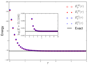
Figure 1: (Color online) Energy versus imaginary time during projection in the Kitaev model. The lattice size $L_{1}$ is $100$, and model parameters are $t=1.0$, $\Delta=2.0$, and $\mu=-3.2$. A time step $\Delta\tau=0.01$ was used. Results from propagating product states are numerically the same as those from propagating Thouless states. The mixed estimator and the growth estimator are consistent with each other, and converge to the exact answer for sufficiently large $\tau$. The inset shows results for $\tau$ from $2$ to $10$, with log-scale of the energy.

As shown in Fig. 1, the computed energies from product state and Thouless state are numerically equivalent, and both converge to the exact ground-state result at large $\tau$. (We use a subscript “$p$” or “$t$” to indicate results from projection of product state or Thouless state, respectively. For example, $E_{p}^{M}(\tau)$ means the mixed estimator by propagating in the product state form, while $E_{t}^{G}(\tau)$ means growth estimator by propagating the Thouless state form.) In these tests, we chose a random wave function as the initial and trial wave function $|\psi_{T}\rangle$, which was first set in the product form, and then mapped to the Thouless form. The growth estimator has a small deviation with the mixed estimator at small imaginary times, which results from the Trotter error from the nonzero time step size $\Delta\tau$. The deviation vanishes at large $\tau$ when $|\psi(\tau)\rangle$ becomes the exact ground state. In Fig. 2, we show the computed pairing order at different imaginary times. The initial value at $\tau=0.0$ is from the random initial wave function. The result is seen to converge to the exact result at the large $\tau$ limit.

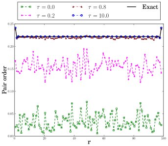
Figure 2: (Color online) Pairing order $\langle c_{r}^{\dagger}c_{r+1}^{\dagger}\rangle$ vs. lattice position $r$ in the Kitaev model computed from $|\psi(\tau)\rangle$ at different projection-times $\tau$, with the same parameters in Fig. 1. The order parameter converges to the exact solution at the large imaginary time limit. For clarity, data in the middle of the lattice are shown at every third value of $r$ for $\tau=10$.

V.2 Hubbard model

We next show the propagation of HFB wave functions in an interacting many-fermion system, the two-dimensional Hubbard model,

$$\hat{H}_{\rm Hub}=-t\sum_{\langle i,j\rangle\sigma}c_{i\sigma}^{\dagger}c_{j\sigma}+U\sum_{i}n_{i\uparrow}n_{i\downarrow}-\mu\sum_{i}(n_{i\uparrow}+n_{i\downarrow})\,.$$ (44)

We will consider periodic lattices with $L_{1}\times L_{2}$ sites in the supercell [i.e., $N=2(L_{1}\times L_{2})$ in the notation of Eq. (12)]. In Eq. (44) the sites are labeled by $i$ and $j$, $c_{i\sigma}^{\dagger}$ and $c_{i\sigma}$ are creation and annihilation operators of an electron of spin $\sigma$ ($=\uparrow$ or $\downarrow$) on the $i$-th lattice site, $t$ is the nearest-neighbor hopping energy, $U$ is the interaction strength, and $\mu$ is the chemical potential. We will use $M_{\sigma}$ to denote the number of particles with spin $\sigma$.

In the attractive Hubbard model ($U<0$), $s$-wave electron pairing is present. Our initial state will take a Bardeen-Cooper-Schrieffer (BCS) wave function, which is a special case of the HFB form. This wave function is then propagated in the AFQMC framework Zhang , and our trial wave function $|\psi_{T}\rangle$ is also of the BCS form. In contrast to Slater determinant initial wave functions (such as Hartree-Fock), the number of particles is not conserved in the BCS wave function. The chemical potential needs to be tuned to reach the targeted number of particles. In Fig. 3, we illustrate the convergence of the QMC propagations of the BCS wave function, and how the expectation value of the particle number varies as the chemical potential is varied. (Our calculations are in the $S_{z}=0$ sector, with $M_{\uparrow}=M_{\downarrow}$.) QMC energies are consistent with exact diagonalization (ED) results, as shown in Table 1. We also compute the pairing correlation function Shi et al. (2015)

$$P_{\rm corr}(i)=\langle c_{0\uparrow}^{\dagger}c_{0\downarrow}^{\dagger}c_{i\downarrow}c_{i\uparrow}\rangle\,.$$ (45)

This requires the full estimator which is implemented by back-propagation in the branching randowm walk approach or by direct measurement at the middle portions of the path in the path integral formula. Here we used the latter Shi et al. (2015); Shi and Zhang (2016). QMC pairing correlation functions are benchmarked against ED results in Fig. 4 for different numbers of particles.

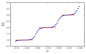
Figure 3: (Color online) QMC calculations by projecting BCS random walkers. Average particle number (for $\uparrow$-electrons) is shown versus chemical potential. The lattice size is $4\times 4$, and model parameters are $t=1.0$, $U=-12.0$. A imaginary-time step of $\Delta\tau=0.01$ was chosen, with projection time $\beta=64t$. Our BCS initial wave function has $\langle M_{\uparrow}\rangle=2.0$. The algorithm converges to different densities as $\mu$ is varied and gives accurate results. The plateaus indicate integer particle numbers.

Table 1: Kinetic, interaction, and total energies from QMC and ED. Three QMC calculations from the middle of the plateaus in Fig. 3 are shown, with $\mu=-0.65$, $-0.55$, and $-0.45$ respectively, which are compared with ED results for fixed particle numbers. The QMC total energy is $\langle\hat{H}_{\rm Hub}+\mu(M_{\uparrow}+M_{\downarrow})\rangle$. QMC statistical error bars are on the last digit and shown in parentheses.

$(M_{\uparrow},M_{\downarrow})$	K		V		E
	ED	QMC	ED	QMC	ED	QMC
$(1,1)$	-2.995	-2.997(3)	-10.42	-10.43(2)	-13.41	-13.42(2)
$(2,2)$	-5.318	-5.320(3)	-21.30	-21.33(2)	-26.62	-26.65(2)
$(3,3)$	-7.162	-7.167(4)	-32.46	-32.42(3)	-39.62	-39.59(3)

The new method affords an advantage in the study of electron pairing correlations, since it allows one to directly treat a Hamiltonian which contains a pairing field. In standard QMC calculations of the Hubbard model (either attractive as in the present case, or repulsive in which the $d$-wave pairing correlation is especially of interest), the Hamiltonian does not break particle number symmetry, which makes it difficult to directly measure a pairing order parameter, $\langle c_{\uparrow}^{\dagger}c_{\downarrow}^{\dagger}\rangle$. Typically one instead measures the pairing correlation function in Eq. (45).

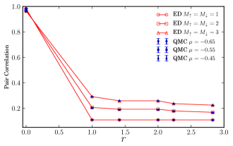
Figure 4: (Color online) Pairing correlation functions computed from QMC and ED. The chemical potential is tuned in QMC to match particle numbers in the ED calculations. Same run parameters are used as in Fig. 3 and Table 1. QMC statistical error bars are smaller than symbol size.

If the order parameter is small, $P_{\rm corr}(i)$ will be much smaller since it is related to the square of the order parameter at large separation $i$. This makes the task of detecting order especially challenging. An alternative way to calculate order parameters is to apply a small pinning field in the Hamiltonian, and detect the order induced by the pinning field Wang et al. (2014); Assaad and Herbut (2013). For pairing we could now apply

$$\hat{H}^{\prime}=\hat{H}_{\rm Hub}+\sum_{i}\frac{h_{i}}{2}(c_{i\uparrow}^{\dagger}c_{i\downarrow}^{\dagger}+c_{i\downarrow}c_{i\uparrow})\,,$$ (46)

where the pairing fields $h_{i}$ will be non-zero only in a small local region (two neighboring sites in the present case). Using the technique described in this paper, we can solve the above Hamiltonian for the Hubbard model with a pairing pinning field. This was done for up to $16\times 16$ lattices to obtain the $1s$ paring order parameter. As illustrated in Fig. 3, the use of a pinning field provides a way to measure pairing order with excellent accuracy. (A more detailed study with finite-size scaling will be required to determine the precise value in the thermodynamic limit.)

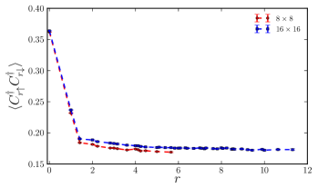
Figure 5: (Color online) Pairing order versus distance. The lattice sizes are $8\times 8$ and $16\times 16$, with total number of particles tuned to $10$ and $40$, respectively. The model parameters are $t=1.0$ and $U=-8.0$. We choose a time step $\Delta\tau=0.01$, and projection time $\beta=64$. Pinning field is put on two neighboring sites (0,0) and (1,0), with $h_{i}=1$.

VI Discussion and Summary

For clarity, we have separated the two forms of HFB states, the product state and the Thouless state, in the discussion of the technical ingredients. The former is more general, while the latter is restricted to fully paired states but gives more compact representations. Of course they can be mixed and used together as needed, both in theory and in numerical implementation. A limitation is that we have not implemented or discussed the case of unpaired fermions, or when the product in Eq. (10) is restricted to a subset of the $N$ quasi-particle operators. We will leave this to a future study.

In Appendix B, we discuss the special example of propagating singlet-pairing BCS wave functions, and write out explicit formulas for the “mixed” overlap and Green’s functions between a BCS wave function and a Slater determinant. This particular case is useful in the study of Fermi gases, for example, where a charge form of the HS decomposition can be used to decouple the attractive short-range interaction but a BCS trial wave function greatly improves the efficiency Carlson et al. (2011). In this form, the energy can be computed straightforwardly with the mixed estimate, but observables require propagating the BCS trial wave function, and keeping it numerically stable.

We have presented the method and formalism in this paper so that they are invariant to whether the Metropolis or the branching random walk method of sampling is used, or whether a sign problem is present or not. The two examples studied in Sec. V are sign-problem-free. When there is a sign or phase problem, it is straightforward to apply a constraint to control it approximately. The constraint is imposed in the branching random walk framework of AFQMC, requiring the calculation of the overlap with $|\psi_{T}\rangle$, and the force bias which is given by the mixed Green’s functions. Both of these ingredients have been discussed and can be applied straightforwardly.

In summary, we have presented the computational ingredients to carry out many-body calculations in interacting fermion systems in the presence of pairing fields. All aspects required to set up a full QMC calculations in such systems are described. Components of the formalism presented may also be useful in other theoretical and computational contexts and can be adopted. We illustrated the method in two situations where propagating a BCS or HFB wave function becomes advantageous or even necessary, namely in model Hamiltonians without $U(1)$ symmetry, or with standard electronic Hamiltonians when a pairing field term is added to induce superconducting correlations. Related situations include the study of Majorana fermions, or in embedding calculations of standard electronic systems where an impurity is coupled to a bath described by a mean-field solution that may have electron pairing present.

After we have completed a draft of the present work, we became aware of Ref. Juillet et al. (2016) which discusses a related approach.

VII Acknowledgments

We are grateful to Dr. S. Chiesa for many contributions in early stages of this work. We thank Garnet Chan, Simone Chiesa, Mingpu Qin, Peter Rosenberg, and Bo-xiao Zheng for valuable discussions. This work was supported by NSF (Grant no. DMR-1409510) and the Simons Foundation. Computing was carried out at at the Extreme Science and Engineering Discovery Environment (XSEDE), which is supported by National Science Foundation grant number ACI-1053575, and at the computational facilities at William & Mary.

Appendix A Additional notations and formulas

We first define a matrix representation which will be used throughout the text. Consider a general bilinear operator,

$$\hat{O}=\sum_{ij}^{N}t_{ij}c_{i}^{\dagger}c_{j}+\sum_{i>j}^{N}\Delta_{ij}c_{i}c_{j}+\sum_{i>j}^{N}\widetilde{\Delta}_{ij}c_{i}^{\dagger}c_{j}^{\dagger}+\eta,$$ (47)

where $t$, $\Delta$, and $\widetilde{\Delta}$ are corresponding $N\times N$ matrices, and $\eta$ is a constant. Note that $\hat{O}$ can be non-Hermition. The matrix representation of $\exp(\hat{O})$ is

$$\exp(\mathbb{O})=\exp\begin{pmatrix}t&\widetilde{\Delta}\\ \Delta&-t^{T}\end{pmatrix},$$ (48)

which does not depend on $\eta$, and we denote its explicit form as

$$\exp(\mathbb{O})=\begin{pmatrix}\mathbb{K}&\mathbb{M}\\ \mathbb{K}&\mathbb{N}\end{pmatrix}.$$ (49)

Linear Transformation of Quas-particle Operators. An arbitrary quas-particle operator $\gamma$ has the form

$$\gamma=\begin{pmatrix}c^{\dagger}&c\end{pmatrix}\begin{pmatrix}v\\ u\end{pmatrix},$$ (50)

with $v=\begin{pmatrix}v_{1}&v_{2}&\dots&v_{N}\end{pmatrix}^{T}$ and $u=\begin{pmatrix}u_{1}&u_{2}&\dots&u_{N}\end{pmatrix}^{T}$. It can be proven that

$$\exp(\hat{O})\gamma\exp(-\hat{O})=\gamma^{\prime},$$ (51)

where $\gamma^{\prime}$ is built from $v^{\prime}$ and $u^{\prime}$ with

$$\begin{pmatrix}v^{\prime}\\ u^{\prime}\end{pmatrix}=\exp(\mathbb{O})\begin{pmatrix}v\\ u\end{pmatrix}.$$ (52)

To prove the above, we use the expansion

$$\exp(\hat{O})\gamma\exp(-\hat{O})=\gamma+[\hat{O},\gamma]+\frac{1}{2!}[\hat{O},[\hat{O},\gamma]]+\cdots.$$ (53)

With commutation relations $[\hat{O},c_{j}^{\dagger}]=(c^{\dagger}t)_{j}+(c\Delta)_{j}$ and $[\hat{O},c_{j}]=(c^{\dagger}\widetilde{\Delta})_{j}+(c(-t^{T}))_{j}$, we obtain

$$[\hat{O},\gamma]=\begin{pmatrix}c^{\dagger}&c\end{pmatrix}\begin{pmatrix}t&\widetilde{\Delta}\\ \Delta&-t^{T}\end{pmatrix}\begin{pmatrix}v\\ u\end{pmatrix},$$ (54)

and

$$[\hat{O},[\hat{O},\gamma]]=\begin{pmatrix}c^{\dagger}&c\end{pmatrix}\begin{pmatrix}t&\widetilde{\Delta}\\ \Delta&-t^{T}\end{pmatrix}^{2}\begin{pmatrix}v\\ u\end{pmatrix}.$$ (55)

The right hand side of Eq. (53) thus gives

$$\gamma^{\prime}=\begin{pmatrix}c^{\dagger}&c\end{pmatrix}\exp\begin{pmatrix}t&\widetilde{\Delta}\\ \Delta&-t^{T}\end{pmatrix}\begin{pmatrix}v\\ u\end{pmatrix}.$$ (56)

Expansion of Exponential Operators. Following Hara and Iwasaki Hara and Iwasaki (1979), we can expand $\exp(\hat{O})$ to three one-body operators,

$$\exp(\hat{O}) = \exp(\frac{1}{2}c^{\dagger}\mathbb{Z}c^{\dagger T})\exp(c^{\dagger}\mathbb{X}c^{T})\exp(\frac{1}{2}c\mathbb{Y}c^{T})\times$$ (57)

$$\langle 0|\exp(\hat{O})|0\rangle.$$

With the help of matrix representation in Eq. (49), we have

$$\mathbb{Z}=\mathbb{M}\mathbb{N}^{-1},\mathbb{X}=\ln(\mathbb{K}),\mathbb{Y}=\mathbb{N}^{-1}\mathbb{L}.$$ (58)

We can also prove

$$\langle 0|\exp(\hat{O})|0\rangle=\sqrt{\det(\mathbb{N})}\exp[\frac{1}{2}\operatorname{Tr}(t)+\eta].$$ (59)

Compression of Exponential Operators. When we have an operator created by multiplying exponentials of one-body operators

$$\hat{O}_{3}=\log[\exp(\hat{O}_{1})\exp(\hat{O}_{2})],$$ (60)

$\hat{O}_{3}$ is still a general one-body operator according to Baker-Campbell-Hausdorff formula. Its matrix representation is

$$\exp(\mathbb{O}_{3})=\exp(\mathbb{O}_{1})\exp(\mathbb{O}_{2}),$$ (61)

which can be proven by linear transformation relation in Eq. (51),

$$\gamma^{\prime\prime} = \exp(\hat{O}_{3})\gamma\exp(-\hat{O}_{3})$$ (62)

$$= \exp(\hat{O}_{1})[\exp(\hat{O}_{2})\gamma\exp(-\hat{O}_{2})]\exp(-\hat{O}_{1}),$$

where $\gamma^{\prime\prime}$ is built from $v^{\prime\prime}$, $u^{\prime\prime}$ by

$$\begin{pmatrix}v^{\prime\prime}\\ u^{\prime\prime}\end{pmatrix} = \exp(\mathbb{O}_{1})\exp(\mathbb{O}_{2})\begin{pmatrix}v\\ u\end{pmatrix}$$ (63)

$$= \exp(\mathbb{O}_{3})\begin{pmatrix}v\\ u\end{pmatrix}.$$

The matrix relations above define everything up to a proportionality constant. The constant prefactor can be determined from

$$\langle 0|\exp(\hat{O}_{3})|0\rangle=\langle 0|\exp(\hat{O}_{1})\exp(\hat{O}_{2})|0\rangle.$$ (64)

The right-hand side can be calculated by expanding $\exp(\hat{O}_{1})$ and $\exp(\hat{O}_{2})$ as in Eq. (57), which leads to overlap of two Thouless state wave functions.

Phase of the HFB State After Propagation. The phase factor of the product state after propagation is determined by Eq. (22). If we have $|\phi\rangle$, the eigenstate of $\hat{O}$:

$$\hat{O}|\phi\rangle=\bar{O}|\phi\rangle,$$ (65)

it is easy to calculate $\alpha$,

$$\alpha=\exp(\bar{O})\frac{\langle\phi|\prod_{i}\beta_{i}|0\rangle}{\langle\phi|\prod_{i}\beta_{i}^{\prime}|0\rangle}\,,$$ (66)

which only involves two overlaps of HFB wave functions. Alternatively, if we choose $|\phi\rangle$ to be the true vacuum, we can apply Eq. (57) to expand $\exp(\hat{O})$:

$$\alpha=\langle 0|\exp(\hat{O})|0\rangle\frac{\langle 0|\exp(\frac{1}{2}c\mathbb{Y}c^{T})\prod_{i}\beta_{i}|0\rangle}{\langle 0|\prod_{i}\beta_{i}^{\prime}|0\rangle}.$$ (67)

Exchanging the exponential operator to the right, we obtain

$$\exp(\frac{1}{2}c\mathbb{Y}c^{T})\prod_{i}\beta_{i}|0\rangle = \prod_{i}\beta_{i}^{\prime\prime}\exp(\frac{1}{2}c\mathbb{Y}c^{T})|0\rangle$$ (68)

$$= \prod_{i}\beta_{i}^{\prime\prime}|0\rangle,$$ (69)

so that $\alpha$ can be determined by the overlaps between the true vacumm and HFB states,

$$\alpha=\langle 0|\exp(\hat{O})|0\rangle\frac{\langle 0|\prod_{i}\beta_{i}^{\prime\prime}|0\rangle}{\langle 0|\prod_{i}\beta_{i}^{\prime}|0\rangle}.$$ (70)

The phase in Thouless state is determined by Eq. (37). When $|\phi\rangle$ is chosen to be the true vacuum, we can expand $\exp(\hat{O})$ as in Eq. (53),

$$\alpha=\langle 0|\exp(\hat{O})|0\rangle\langle 0|\exp(\frac{1}{2}c\mathbb{Y}c^{T})|\psi_{t}\rangle\,,$$ (71)

which is given by the verlap of two Thouless state wave functions.

Appendix B The special case of an HFB wave function and a Slater determinant

A special case of our discussions is an HFB wave function with a Slater determinant (SD). Here the HFB wave function is

$$|\psi\rangle=\exp(\frac{1}{2}c^{\dagger}\mathbb{Z}(c^{\dagger})^{T})|0\rangle,$$ (72)

and the SD wave function is

$$|\phi\rangle=\prod_{i}^{M}\phi_{i}^{\dagger}|0\rangle,$$ (73)

with $\phi_{i}^{\dagger}=c^{\dagger}\phi_{i}$, and $M$ being the number of fermions.

The overlap between the HFB and SD wave functions is determined by

$$\langle\psi|\phi\rangle=\mathrm{pf}(\phi^{T}\mathbb{Z}^{*}\phi).$$ (74)

Setting $Q=\phi^{T}\mathbb{Z}^{\dagger}\phi$, we have the Green’s functions,

$$\rho_{ij}=\frac{\langle\psi|c_{i}^{\dagger}c_{j}|\phi\rangle}{\langle\psi|\phi\rangle} = (\mathbb{Z}^{\dagger}\phi Q^{-1}\phi^{T})_{ji},$$

$$\kappa_{ij}=\frac{\langle\psi|c_{i}c_{j}|\phi\rangle}{\langle\psi|\phi\rangle} = (-\phi Q^{-1}\phi^{T})_{ij},$$

$$\overline{\kappa}_{ij}=\frac{\langle\psi|c_{i}^{\dagger}c_{j}^{\dagger}|\phi\rangle}{\langle\psi|\phi\rangle} = (-\mathbb{Z}^{\dagger}+\mathbb{Z}^{\dagger}\phi Q^{-1}\phi^{T}\mathbb{Z}^{\dagger})_{ij}~{}.$$ (75)

Projected HFB wave function. In situations where it is desirable to preserve $U(1)$ symmetry projected HFB (PHFB) wave function becomes useful. For a fixed number of particles $M$, the PHFB wave function is

$$|\psi_{\mathrm{PHFB}}\rangle=\frac{1}{2^{M/2}{(M/2)}!}(c^{\dagger}Zc^{\dagger})^{M/2}|0\rangle.$$ (76)

The overlap between a PHFB and an SD is the same as Eq. (74) and the Green’s functions are the same as Eq. (B).

The propagator for PHFB should not break $U(1)$ symmetry. Let us set $\Delta$ and $\widetilde{\Delta}$ to zero in Eq. (47). The new PHFB wave function after propagation is

$$|\psi^{\prime}_{\mathrm{PHFB}}\rangle=\exp(\hat{O})|\psi_{\mathrm{PHFB}}\rangle,$$ (77)

and $Z^{\prime}$ in $|\psi^{\prime}_{\mathrm{PHFB}}\rangle$ is

$$Z^{\prime}=\exp(t)Z\exp(t^{T}).$$ (78)

Spin-$1/2$ model with singlet pairing. Let us consider spin-$1/2$ fermions in a basis of size $N_{\rm basis}$. If pairing is only between opposite spins, $\mathbb{Z}$ is specialized to

$$\mathbb{Z}=\begin{pmatrix}0&\mathbb{Z}_{0}\\ -\mathbb{Z}_{0}^{T}&0\end{pmatrix},$$ (79)

where $\mathbb{Z}_{0}$ is an $N_{\rm basis}\times N_{\rm basis}$ matrix. If $SU(2)$ symmetry is present, $\mathbb{Z}_{0}$ is Hermition. The SD wave function is in block diagonal form

$$\phi=\begin{pmatrix}\phi_{\uparrow}&0\\ 0&\phi_{\downarrow}\end{pmatrix},$$ (80)

where $\phi_{\uparrow}$ and $\phi_{\downarrow}$ are $N_{\rm basis}\times M/2$ matrices.

The overlap between the HFB and SD is reduced to a determinant

$$\langle\psi|\phi\rangle=(-1)^{M/2\,(M/2-1)/2}\det(\phi_{\downarrow}^{T}\mathbb{Z}_{0}^{\dagger}\phi_{\uparrow}),$$ (81)

which can be calculated efficiently. Note that we can ignore the overall sign here if the number of particles is fixed in the calculation. If we set $Q_{0}=\phi_{\downarrow}^{T}\mathbb{Z}_{0}^{\dagger}\phi_{\uparrow}$, the nonzero Green’s functions are

$$\frac{\langle\psi|c_{i\uparrow}^{\dagger}c_{j\uparrow}|\phi\rangle}{\langle\psi|\phi\rangle} = (\mathbb{Z}_{0}^{*}\phi_{\downarrow}(Q_{0}^{T})^{-1}\phi_{\uparrow}^{T})_{ij},$$

$$\frac{\langle\psi|c_{i\downarrow}^{\dagger}c_{j\downarrow}|\phi\rangle}{\langle\psi|\phi\rangle} = (\mathbb{Z}_{0}^{\dagger}\phi_{\uparrow}Q_{0}^{-1}\phi_{\downarrow}^{T})_{ij},$$

$$\frac{\langle\psi|c_{i\uparrow}c_{j\downarrow}|\phi\rangle}{\langle\psi|\phi\rangle} = (-\phi_{\uparrow}Q_{0}^{-1}\phi_{\downarrow}^{T})_{ij},$$

$$\frac{\langle\psi|c_{i\uparrow}^{\dagger}c_{j\downarrow}^{\dagger}|\phi\rangle}{\langle\psi|\phi\rangle} = (\mathbb{Z}_{0}^{*}-\mathbb{Z}_{0}^{*}\phi_{\downarrow}(Q_{0}^{T})^{-1}\phi_{\uparrow}^{T}\mathbb{Z}_{0}^{*})_{ij}~{}.$$ (82)

The corresponding projected HFB wave function is similar to Eq. (76),

$$|\psi_{\mathrm{PHFB}}\rangle=\frac{1}{(M/2)!}(c_{\uparrow}^{\dagger}Z_{0}c_{\downarrow}^{\dagger})^{M/2}|0\rangle,$$ (83)

where $c_{\uparrow}^{\dagger}$ and $c_{\downarrow}^{\dagger}$ are the same as $c^{\dagger}$ except for the spin index. The general operator in Eq. (47) has the form

$$t=\begin{pmatrix}t_{\uparrow}&0\\ 0&t_{\downarrow}\end{pmatrix},$$ (84)

with $\Delta$ and $\widetilde{\Delta}$ equal to zero again. After propagation, the new $Z_{0}^{\prime}$ is given by

$$Z_{0}^{\prime}=\exp(t_{\uparrow})Z_{0}\exp(t_{\downarrow}^{T}).$$ (85)

For a system with $SU(2)$ symmetry, we have $t_{\uparrow}=t_{\downarrow}^{*}$ and $Z_{0}=U_{0}D_{0}U_{0}^{\dagger}$, where $U_{0}$ is a unitary matrix and $D_{0}$ is a diagonal matrix. The propagation is

$$Z_{0}^{\prime}=(\exp(t_{\uparrow})U_{0})D_{0}(\exp(t_{\uparrow})U_{0})^{\dagger},$$ (86)

and $Z_{0}^{\prime}$ will remain Hermition. The propagation can be thought of as $U_{0}^{\prime}=\exp(t_{\uparrow})U_{0}$, which is similar to propagating an SD wave function. Note that maintaining numerical stability in the propagation will likely require additional investigation in these situations.

References

- (1) P. Ring and P. Schuck, The Nuclear Many-Body Problem (SpringerVerlag, New York, 1980).
- Scuseria et al. (2011) G. E. Scuseria, C. A. Jiménez-Hoyos, T. M. Henderson, K. Samanta, and J. K. Ellis, The Journal of Chemical Physics 135, 124108 (2011), URL http://scitation.aip.org/content/aip/journal/jcp/135/12/10.1063/1.3643338.
- Bertsch and Robledo (2012) G. F. Bertsch and L. M. Robledo, Phys. Rev. Lett. 108, 042505 (2012), URL http://link.aps.org/doi/10.1103/PhysRevLett.108.042505.
- Tahara and Imada (2008) D. Tahara and M. Imada, Journal of the Physical Society of Japan 77, 114701 (2008), eprint http://dx.doi.org/10.1143/JPSJ.77.114701, URL http://dx.doi.org/10.1143/JPSJ.77.114701.
- Bajdich et al. (2006) M. Bajdich, L. Mitas, G. Drobný, L. K. Wagner, and K. E. Schmidt, Phys. Rev. Lett. 96, 130201 (2006), URL http://link.aps.org/doi/10.1103/PhysRevLett.96.130201.
- Casula and Sorella (2003) M. Casula and S. Sorella, The Journal of Chemical Physics 119, 6500 (2003), URL http://scitation.aip.org/content/aip/journal/jcp/119/13/10.1063/1.1604379.
- Carlson et al. (2011) J. Carlson, S. Gandolfi, K. E. Schmidt, and S. Zhang, Phys. Rev. A 84, 061602 (2011), URL http://link.aps.org/doi/10.1103/PhysRevA.84.061602.
- Zheng and Chan (2016) B.-X. Zheng and G. K.-L. Chan, Phys. Rev. B 93, 035126 (2016), URL http://link.aps.org/doi/10.1103/PhysRevB.93.035126.
- (9) S. Zhang, Auxiliary-Field Quantum Monte Carlo for Correlated Electron Systems, Vol. 3 of Emergent Phenomena in Correlated Matter: Modeling and Simulation, Ed. E. Pavarini, E. Koch, and U. Schollwöck (Verlag des Forschungszentrum Jülich, 2013).
- (10) F. F. Assaad, Quantum Monte Carlo Methods on Lattices: The Determinantal method., Lecture notes of the Winter School on Quantum Simulations of Complex Many-Body Systems: From Theory to Algorithms. Publication Series of the John von Neumann Institute for Computing (NIC). NIC series Vol. 10. ISBN 3-00-009057-6 Pages 99-155.
- Zhang et al. (1995) S. Zhang, J. Carlson, and J. E. Gubernatis, Phys. Rev. Lett. 74, 3652 (1995).
- Zhang and Krakauer (2003) S. Zhang and H. Krakauer, Phys. Rev. Lett. 90, 136401 (2003), URL http://link.aps.org/doi/10.1103/PhysRevLett.90.136401.
- Wouters et al. (2014) S. Wouters, B. Verstichel, D. Van Neck, and G. K.-L. Chan, Phys. Rev. B 90, 045104 (2014), URL http://link.aps.org/doi/10.1103/PhysRevB.90.045104.
- Zhang et al. (1997) S. Zhang, J. Carlson, and J. E. Gubernatis, Phys. Rev. B 55, 7464 (1997).
- Purwanto and Zhang (2004) W. Purwanto and S. Zhang, Phys. Rev. E 70, 056702 (2004), URL http://link.aps.org/doi/10.1103/PhysRevE.70.056702.
- Shi and Zhang (2016) H. Shi and S. Zhang, Phys. Rev. E 93, 033303 (2016), URL http://link.aps.org/doi/10.1103/PhysRevE.93.033303.
- Shi et al. (2015) H. Shi, S. Chiesa, and S. Zhang, Phys. Rev. A 92, 033603 (2015), URL http://link.aps.org/doi/10.1103/PhysRevA.92.033603.
- Shi and Zhang (2013) H. Shi and S. Zhang, Phys. Rev. B 88, 125132 (2013), URL http://link.aps.org/doi/10.1103/PhysRevB.88.125132.
- Shi et al. (2014) H. Shi, C. A. Jiménez-Hoyos, R. Rodríguez-Guzmán, G. E. Scuseria, and S. Zhang, Phys. Rev. B 89, 125129 (2014), URL http://link.aps.org/doi/10.1103/PhysRevB.89.125129.
- Bonnard and Juillet (2013) J. Bonnard and O. Juillet, Phys. Rev. Lett. 111, 012502 (2013), URL http://link.aps.org/doi/10.1103/PhysRevLett.111.012502.
- Robledo (2009) L. M. Robledo, Phys. Rev. C 79, 021302 (2009), URL http://link.aps.org/doi/10.1103/PhysRevC.79.021302.
- González-Ballestero et al. (2011) C. González-Ballestero, L. Robledo, and G. Bertsch, Computer Physics Communications 182, 2213 (2011), ISSN 0010-4655, URL http://www.sciencedirect.com/science/article/pii/S0010465511001627.
- Onishi and Yoshida (1966) N. Onishi and S. Yoshida, Nuclear Physics 80, 367 (1966), ISSN 0029-5582, URL http://www.sciencedirect.com/science/article/pii/0029558266900964.
- Balian and Brezin (1969) R. Balian and E. Brezin, Il Nuovo Cimento B (1965-1970) 64, 37 (1969), ISSN 1826-9877, URL http://dx.doi.org/10.1007/BF02710281.
- Kitaev (2001) A. Y. Kitaev, Physics-Uspekhi 44, 131 (2001).
- Wang et al. (2014) D. Wang, Y. Li, Z. Cai, Z. Zhou, Y. Wang, and C. Wu, Phys. Rev. Lett. 112, 156403 (2014), URL http://link.aps.org/doi/10.1103/PhysRevLett.112.156403.
- Assaad and Herbut (2013) F. F. Assaad and I. F. Herbut, Phys. Rev. X 3, 031010 (2013), URL http://link.aps.org/doi/10.1103/PhysRevX.3.031010.
- Juillet et al. (2016) O. Juillet, A. Leprévost, J. Bonnard, and R. Frésard, ArXiv e-prints (2016), eprint 1610.08022.
- Hara and Iwasaki (1979) K. Hara and S. Iwasaki, Nuclear Physics A 332, 61 (1979), ISSN 0375-9474, URL http://www.sciencedirect.com/science/article/pii/0375947479900940.