D-wave charmed and bottomed baryons from QCD sum rules

Abstract

We study the $D$-wave charmed baryons of $SU(3)$ flavor $\mathbf{\bar{3}}_{F}$ using the method of QCD sum rules in the framework of heavy quark effective theory. We find that the $\Lambda_{c}(2880)$, $\Xi_{c}(3055)$ and $\Xi_{c}(3080)$ can be well described by the $D$-wave $SU(3)$ $\mathbf{\bar{3}}_{F}$ charmed baryon multiplets of $J^{P}=3/2^{+}$ and $5/2^{+}$, which contain two $\lambda$-mode orbital excitations, i.e., the $\Lambda_{c}(2880)$ has $J^{P}=5/2^{+}$, and the $\Xi_{c}(3055)$ and $\Xi_{c}(3080)$ have $J^{P}=3/2^{+}$ and $5/2^{+}$, respectively. Our results also suggest that the $\Lambda_{c}(2880)$ has a partner state, the $\Lambda_{c}(3/2^{+})$ of $J^{P}=3/2^{+}$. Its mass is around $2.81^{+0.33}_{-0.18}$ GeV, and the mass difference between it and the $\Lambda_{c}(2880)$ is $28^{+45}_{-24}$ MeV. We also evaluate the masses of their bottom partners.

I Introduction

In the past years important experimental progresses have been made in the field of charmed baryons. All the $1S$ charmed baryons have been well established pdg . Moreover, the $1P$ states $\Lambda_{c}(2595)$, $\Lambda_{c}(2625)$, $\Xi_{c}(2790)$ and $\Xi_{c}(2815)$ have also been well observed and complete two $SU(3)$ flavor $\mathbf{\bar{3}}_{F}$ multiplets of $J^{P}=1/2^{-}$ and $3/2^{-}$ Albrecht:1993pt ; Frabetti:1993hg ; Edwards:1994ar ; Alexander:1999ud . Besides them, there still exist many higher states, i.e., the $\Lambda_{c}(2765)$ ($J^{P}=?^{?}$) Artuso:2000xy , the $\Lambda_{c}(2880)$ ($J^{P}=5/2^{+}$) Artuso:2000xy , the $\Lambda_{c}(2940)$ ($J^{P}=?^{?}$) Aubert:2006sp ; Abe:2006rz , the $\Sigma_{c}(2800)$ ($J^{P}=?^{?}$) Mizuk:2004yu , the $\Xi_{c}(2930)$ ($J^{P}=?^{?}$) Aubert:2007eb , the $\Xi_{c}(2980)$ ($J^{P}=?^{?}$) Chistov:2006zj ; Yelton:2016fqw , the $\Xi_{c}(3055)$ ($J^{P}=?^{?}$) Aubert:2007dt ; Kato:2016hca , the $\Xi_{c}(3080)$ ($J^{P}=?^{?}$) Chistov:2006zj , and the $\Xi_{c}(3123)$ ($J^{P}=?^{?}$) Aubert:2007dt . Some of them may belong to the $1P$ $SU(3)$ flavor $\mathbf{6}_{F}$ multiplets, while some of them are good $D$-wave charmed baryon candidates. Especially, in this paper we shall concentrate on the $\Lambda_{c}(2880)$, $\Xi_{c}(3055)$ and $\Xi_{c}(3080)$, which were proposed (or detailly discussed) in Refs. Ebert:2011kk ; Chen:2014nyo ; Cheng:2015rra to be $1D$ charmed baryons of the quantum numbers $J^{P}=5/2^{+}$, $3/2^{+}$ and $5/2^{+}$, respectively. More assignments can be found in Refs. Cheng:2006dk ; Garcilazo:2007eh ; Gerasyuta:2007un ; Zhong:2007gp ; Selem:2006nd , and we refer to reviews Chen:2016spr ; Cheng:2015rra for their recent progress.

The charmed baryons have been investigated using many phenomenological methods/models in the past two decades, including various quark models Capstick:1986bm ; Ebert:2007nw ; Ortega:2012cx ; Shah:2016nxi ; Thakkar:2016dna , the combined expansion in $1/m_{Q}$ and $1/N_{c}$ Jenkins:1996de , the hyperfine interaction Copley:1979wj ; Karliner:2008sv , the Feynman-Hellmann theorem Roncaglia:1995az , the variational approach Roberts:2007ni , the unitarized dynamical model GarciaRecio:2012db , the extended local hidden gauge approach Liang:2014eba , the unitarized chiral perturbation theory Lu:2014ina , and the Lattice QCD Bowler:1996ws ; Burch:2008qx ; Brown:2014ena , etc. Their pionic decays and related pion induced reactions have also been studied in Refs. Zhong:2007gp ; Nagahiro:2016nsx ; Kim:2014qha . See reviews in Refs. Korner:1994nh ; Bianco:2003vb ; Klempt:2009pi ; Crede:2013sze .

We have also systematically studied the charmed baryons, i.e., the $S$-wave bottom baryons Liu:2007fg , the $P$-wave charmed baryons Chen:2015kpa , and the $P$-wave bottom baryons Mao:2015gya , using the method of QCD sum rules Shifman:1978bx ; Reinders:1984sr in the framework of heavy quark effective theory (HQET) Grinstein:1990mj ; Eichten:1989zv ; Falk:1990yz . This scheme has been successfully applied to study heavy mesons and baryons containing a single heavy quark Bagan:1991sg ; Neubert:1991sp ; Neubert:1993mb ; Broadhurst:1991fc ; Ball:1993xv ; Huang:1994zj ; Dai:1996yw ; Dai:1993kt ; Dai:1996qx ; Colangelo:1998ga ; Dai:2003yg ; Zhou:2014ytp ; Zhou:2015ywa ; Shuryak:1981fza ; Grozin:1992td ; Bagan:1993ii ; Dai:1995bc ; Dai:1996xv ; Groote:1996em ; Zhu:2000py ; Lee:2000tb ; Huang:2000tn ; Wang:2003zp , while other studies using the method of QCD sum rules but not in HQET can be found in Refs. Bagan:1992tp ; Bagan:1991sc ; Duraes:2007te ; Wang:2007sqa ; Chen:2016qju ; Chen:2015moa .

In this paper we study the $D$-wave charmed baryons of $SU(3)$ flavor $\mathbf{\bar{3}}_{F}$ $(\Lambda_{c},\Xi_{c})$ using the method of QCD sum rules within HQET. This paper is organized as follows. First we systematically construct the interpolating currents for the $D$-wave charmed baryons in Sec. II. Then we select some of them to perform the QCD sum rule analysis at both the leading order in Sec. III and the order ${\mathcal{O}}(1/m_{Q})$ in Sec. IV. During the calculations, we shall take the ${\mathcal{O}}(1/m_{c})$ corrections ($m_{c}$ is the heavy quark mass) into account, and extract the chromomagnetic splitting. In Sec. V we perform numerical analyses and discuss the obtained results. A short summary is given in Sec. VI.

II interpolating fields for the $P$-wave charmed baryon

The charmed baryons of $P$- and $D$-waves have been systemically classified in Ref. Chen:2007xf , where their strong decays were systematically investigated using the ${}^{3}P_{0}$ model. The $P$-wave charmed baryon interpolating fields have been systematically constructed in Refs. Chen:2015kpa ; Mao:2015gya using the same notations, i.e., $l_{\rho}$ denotes the orbital angular momentum between the two light quarks and $l_{\lambda}$ denotes the orbital angular momentum between the charm quark and the two-light-quark system.

In this paper we follow the same approach of Refs. Chen:2015kpa ; Mao:2015gya , and construct the $D$-wave ($L=2$) charmed baryon interpolating fields. We use the notation $J^{\alpha_{1}\cdots\alpha_{j-1/2}}_{j,P,F,j_{l},s_{l},\rho\rho/\lambda\lambda/\rho\lambda}$ to denote the $D$-wave charmed baryon interpolating field having the total angular momentum $j$ and parity $P$, and belonging to the spin doublet $[F,j_{l},s_{l},\rho\rho/\lambda\lambda/\rho\lambda]$. Here $F$ denotes the $SU(3)$ flavor representation, either $\mathbf{\bar{3}}_{F}$ or $\mathbf{6}_{F}$; $j_{l}$ and $s_{l}$ denote the total angular momentum and spin angular momentum of the light components; $[\rho\rho]$ denotes $l_{\rho}=2$ and $l_{\lambda}=0$, $[\lambda\lambda]$ denotes $l_{\rho}=0$ and $l_{\lambda}=2$, and $[\rho\lambda]$ denotes $l_{\rho}=1$ and $l_{\lambda}=1$. We have the relations $L=l_{\lambda}\otimes l_{\rho}$, $j_{l}=L\otimes s_{l}$ and $j=j_{l}\otimes s_{Q}$, where $s_{Q}=1/2$ is the spin of the heavy quark.

We summarize all the possible configurations of the $D$-wave ($L=2$) charmed baryons in Fig. 1, where $\mathbf{A}$ and $\mathbf{S}$ denote the structure to be antisymmetric and symmetric, respectively. We note that the type $[\rho\lambda]$ ($l_{\rho}=1$ and $l_{\lambda}=1$) can actually have total orbital angular momenta $L=0$, $1$ and $2$, but in this paper we only concentrate on the $L=2$ for the $D$-wave case.

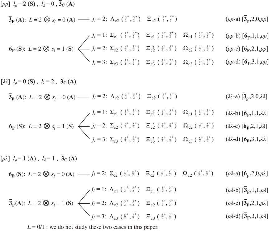
Figure 1: The notations for $D$-wave charmed baryons: $\mathbf{6}_{F}$ ($\mathbf{S}$) and $\mathbf{\bar{3}}_{F}$ ($\mathbf{A}$) denote the $SU(3)$ flavor representations; $\mathbf{\bar{3}}_{C}$ ($\mathbf{A}$) denotes the $SU(3)$ color representation; $s_{l}$ is the spin angular momentum of the two light quarks; $j_{l}=L\otimes s_{l}=l_{\lambda}\otimes l_{\rho}\otimes s_{l}$ is the total angular momentum of the two light quarks.

Generally, the interpolating field for charmed baryons can be written as a combination of a diquark field and a heavy quark field

$$J(x)\sim\epsilon_{abc}\left(q^{aT}(x)\mathbb{C}\Gamma_{1}q^{b}(x)\right)\Gamma_{2}h_{v}^{c}(x)\,,$$ (1)

where $a$, $b$ and $c$ are color indices; $\epsilon_{abc}$ is the totally antisymmetric tensor; the superscript $T$ represents the transpose of the Dirac indices; the matrices $\Gamma_{1,2}$ are Dirac matrices which describe the Lorentz structure; $\mathbb{C}$ is the charge-conjugation operator; $q(x)$ denotes the light quark field at location $x$, and it can be either $u(x)$ or $d(x)$ or $s(x)$; $h_{v}(x)$ denotes the heavy quark field, and we have used the Fierz transformation to move it to the rightmost place. Besides these notations, $\gamma^{t}_{\mu}=\gamma_{\mu}-v\!\!\!/v_{\mu}$, $D_{\mu}=\partial_{\mu}-igA_{\mu}$, $D_{\mu}^{t}=D_{\mu}-(D\cdot v)v_{\mu}$, $v$ is the velocity of the heavy quark, and $g_{t}^{\alpha_{1}\alpha_{2}}=g^{\alpha_{1}\alpha_{2}}-v^{\alpha_{1}}v^{\alpha_{2}}$ is the transverse metric tensor.

To describe the orbital angular momenta, we directly apply two derivatives containing two symmetric Lorentz indices on the light diquark field (see Refs. Chen:2015kpa ; Mao:2015gya ; Zhu:2000py ; Lee:2000tb ; Huang:2000tn ; Wang:2003zp for more details) to construct the $D$-wave diquark fields of the configuration $[\rho\rho/\lambda\lambda/\rho\lambda]$:

$$~{}[\rho\rho]~{}[^{1}D_{2}] : \,l_{\rho}=2~{}(\mathbf{S})\,,\,l_{\lambda}=0\,,\,L=2\,,\,s_{l}=0~{}(\mathbf{A})\,,\,j_{l}=2$$

$$\epsilon_{abc} \times \Big{(}[\mathcal{D}_{\mu_{1}}\mathcal{D}_{\mu_{2}}q^{aT}(x)]\mathbb{C}\gamma_{5}q^{b}(x)-2[\mathcal{D}_{\mu_{1}}q^{aT}(x)]\mathbb{C}\gamma_{5}[\mathcal{D}_{\mu_{2}}q^{b}(x)]+q^{aT}(x)\mathbb{C}\gamma_{5}[\mathcal{D}_{\mu_{1}}\mathcal{D}_{\mu_{2}}q^{b}(x)]\Big{)}+\mu_{1}\leftrightarrow\mu_{2}\,,$$

$$~{}[\rho\rho]~{}[^{3}D_{1/2/3}] : \,l_{\rho}=2~{}(\mathbf{S})\,,\,l_{\lambda}=0\,,\,L=2\,,\,s_{l}=1~{}(\mathbf{A})\,,\,j_{l}=1/2/3$$

$$\epsilon_{abc} \times \Big{(}[\mathcal{D}_{\mu_{1}}\mathcal{D}_{\mu_{2}}q^{aT}(x)]\mathbb{C}\gamma_{\mu}q^{b}(x)-2[\mathcal{D}_{\mu_{1}}q^{aT}(x)]\mathbb{C}\gamma_{\mu}[\mathcal{D}_{\mu_{2}}q^{b}(x)]+q^{aT}(x)\mathbb{C}\gamma_{\mu}[\mathcal{D}_{\mu_{1}}\mathcal{D}_{\mu_{2}}q^{b}(x)]\Big{)}+\mu_{1}\leftrightarrow\mu_{2}\,,$$

$$~{}[\lambda\lambda]~{}[^{1}S_{0}] : \,l_{\rho}=0~{}(\mathbf{S})\,,\,l_{\lambda}=2\,,\,L=2\,,\,s_{l}=0~{}(\mathbf{A})\,,\,j_{l}=2$$

$$\epsilon_{abc} \times \Big{(}[\mathcal{D}_{\mu_{1}}\mathcal{D}_{\mu_{2}}q^{aT}(x)]\mathbb{C}\gamma_{5}q^{b}(x)+2[\mathcal{D}_{\mu_{1}}q^{aT}(x)]\mathbb{C}\gamma_{5}[\mathcal{D}_{\mu_{2}}q^{b}(x)]+q^{aT}(x)\mathbb{C}\gamma_{5}[\mathcal{D}_{\mu_{1}}\mathcal{D}_{\mu_{2}}q^{b}(x)]\Big{)}+\mu_{1}\leftrightarrow\mu_{2}\,,$$

$$~{}[\lambda\lambda]~{}[^{3}S_{1}] : \,l_{\rho}=0~{}(\mathbf{S})\,,\,l_{\lambda}=2\,,\,L=2\,,\,s_{l}=1~{}(\mathbf{A})\,,\,j_{l}=1/2/3$$

$$\epsilon_{abc} \times \Big{(}[\mathcal{D}_{\mu_{1}}\mathcal{D}_{\mu_{2}}q^{aT}(x)]\mathbb{C}\gamma_{\mu}q^{b}(x)+2[\mathcal{D}_{\mu_{1}}q^{aT}(x)]\mathbb{C}\gamma_{\mu}[\mathcal{D}_{\mu_{2}}q^{b}(x)]+q^{aT}(x)\mathbb{C}\gamma_{\mu}[\mathcal{D}_{\mu_{1}}\mathcal{D}_{\mu_{2}}q^{b}(x)]\Big{)}+\mu_{1}\leftrightarrow\mu_{2}\,,$$

$$~{}[\rho\lambda]~{}[^{1}P_{1}] : \,l_{\rho}=1~{}(\mathbf{A})\,,\,l_{\lambda}=1\,,\,L=2\,,\,s_{l}=0~{}(\mathbf{A})\,,\,j_{l}=2$$

$$\epsilon_{abc} \times \Big{(}[\mathcal{D}_{\mu_{1}}\mathcal{D}_{\mu_{2}}q^{aT}(x)]\mathbb{C}\gamma_{5}q^{b}(x)-q^{aT}(x)\mathbb{C}\gamma_{5}[\mathcal{D}_{\mu_{1}}\mathcal{D}_{\mu_{2}}q^{b}(x)]\Big{)}+\mu_{1}\leftrightarrow\mu_{2}\,,$$

$$~{}[\rho\lambda]~{}[^{3}P_{0/1/2}] : \,l_{\rho}=1~{}(\mathbf{A})\,,\,l_{\lambda}=1\,,\,L=2\,,\,s_{l}=1~{}(\mathbf{A})\,,\,j_{l}=1/2/3$$

$$\epsilon_{abc} \times \Big{(}[\mathcal{D}_{\mu_{1}}\mathcal{D}_{\mu_{2}}q^{aT}(x)]\mathbb{C}\gamma_{\mu}q^{b}(x)-q^{aT}(x)\mathbb{C}\gamma_{\mu}[\mathcal{D}_{\mu_{1}}\mathcal{D}_{\mu_{2}}q^{b}(x)]\Big{)}+\mu_{1}\leftrightarrow\mu_{2}\,,$$

$$~{}[\rho\lambda]~{}[\cdots] : \,l_{\rho}=1~{}(\mathbf{A})\,,\,l_{\lambda}=1\,,\,L=0/1\,,\,s_{l}=0/1~{}(\mathbf{A/S})\,,\,j_{l}=0/1/2$$

we do not study these cases in this paper.

In these expressions, we have used $[^{2s_{l}+1}\big{(}l_{\rho}\big{)}_{l_{\rho}\otimes s_{l}}]$ to denote the spin, orbital and total angular momenta of the diquark, where $l_{\lambda}$ (the orbital angular momentum between the charm quark and the diquark) is not taken into account. Especially, $[^{3}D_{1/2/3}]$ means $l_{\rho}\otimes s_{l}$ can be 1, 2 and 3, while $[^{3}P_{0/1/2}]$ means $l_{\rho}\otimes s_{l}$ can be 0, 1 and 2.

Based on these $D$-wave diquark fields, we can construct the $D$-wave ($L=2$) charmed baryons of the configuration $[\rho\rho/\lambda\lambda/\rho\lambda]$:

• $[\rho\rho]$ ($l_{\rho}=2$ ($\mathbf{S}$) and $l_{\lambda}=0$):

  1. $[\mathbf{\bar{3}}_{F},2,0,\rho\rho]$ with $s_{l}=0$ ($\mathbf{A}$) and $j_{l}=2$. Now the diquark has color $\mathbf{\bar{3}}_{C}$ ($\mathbf{A}$) and flavor $\mathbf{\bar{3}}_{F}$ ($\mathbf{A}$), and we obtain a spin doublet $(j^{P}=3/2^{+},5/2^{+})$:

     $$J^{\alpha}_{3/2,+,\mathbf{\bar{3}}_{F},2,0,\rho\rho}(x)$$

     $$= \epsilon_{abc}\Big{(}[\mathcal{D}^{t}_{\mu_{1}}\mathcal{D}^{t}_{\mu_{2}}q^{aT}(x)]\mathbb{C}\gamma_{5}q^{b}(x)-2[\mathcal{D}^{t}_{\mu_{1}}q^{aT}(x)]\mathbb{C}\gamma_{5}[\mathcal{D}^{t}_{\mu_{2}}q^{b}(x)]+q^{aT}(x)\mathbb{C}\gamma_{5}[\mathcal{D}^{t}_{\mu_{1}}\mathcal{D}^{t}_{\mu_{2}}q^{b}(x)]\Big{)}$$

     $$~{}~{}~{}~{}~{}~{}~{}~{}~{}~{}~{}~{}\times\Big{(}{1\over 2}g_{t}^{\mu_{1}\alpha}g_{t}^{\mu_{2}\mu_{4}}+{1\over 2}g_{t}^{\mu_{2}\alpha}g_{t}^{\mu_{1}\mu_{4}}-{1\over 3}g_{t}^{\mu_{1}\mu_{2}}g_{t}^{\mu_{4}\alpha}\Big{)}\times\gamma^{t}_{\mu_{4}}\gamma_{5}h_{v}^{c}(x)\,,$$

     $$J^{\alpha_{1}\alpha_{2}}_{5/2,+,\mathbf{\bar{3}}_{F},2,0,\rho\rho}(x)$$

     $$= \epsilon_{abc}\Big{(}[\mathcal{D}^{t}_{\mu_{1}}\mathcal{D}^{t}_{\mu_{2}}q^{aT}(x)]\mathbb{C}\gamma_{5}q^{b}(x)-2[\mathcal{D}^{t}_{\mu_{1}}q^{aT}(x)]\mathbb{C}\gamma_{5}[\mathcal{D}^{t}_{\mu_{2}}q^{b}(x)]+q^{aT}(x)\mathbb{C}\gamma_{5}[\mathcal{D}^{t}_{\mu_{1}}\mathcal{D}^{t}_{\mu_{2}}q^{b}(x)]\Big{)}$$

     $$~{}~{}~{}~{}~{}~{}~{}~{}~{}~{}~{}~{}\times\Gamma_{t}^{\alpha_{1}\alpha_{2},\mu_{1}\mu_{2}}\times h_{v}^{c}(x)\,,$$

     where $\Gamma_{t}^{\alpha_{1}\alpha_{2},\mu_{1}\mu_{2}}$ is the projection operator projecting into pure spin 2, whose explicit form is given in Appendix A.

  2. $[\mathbf{6}_{F},1,1,\rho\rho]$ with $s_{l}=1$ ($\mathbf{S}$) and $j_{l}=1$. Now the diquark has color $\mathbf{\bar{3}}_{C}$ ($\mathbf{A}$) and flavor $\mathbf{6}_{F}$ ($\mathbf{S}$), and we obtain a spin doublet $(1/2^{+},3/2^{+})$:

     $$J_{1/2,+,\mathbf{6}_{F},1,1,\rho\rho}(x)$$

     $$= \epsilon_{abc}\Big{(}[\mathcal{D}^{t}_{\mu_{1}}\mathcal{D}^{t}_{\mu_{2}}q^{aT}(x)]\mathbb{C}\gamma^{t}_{\mu_{3}}q^{b}(x)-2[\mathcal{D}^{t}_{\mu_{1}}q^{aT}(x)]\mathbb{C}\gamma^{t}_{\mu_{3}}[\mathcal{D}^{t}_{\mu_{2}}q^{b}(x)]+q^{aT}(x)\mathbb{C}\gamma^{t}_{\mu_{3}}[\mathcal{D}^{t}_{\mu_{1}}\mathcal{D}^{t}_{\mu_{2}}q^{b}(x)]\Big{)}$$

     $$~{}~{}~{}~{}~{}~{}~{}~{}~{}~{}~{}~{}\times\Big{(}g_{t}^{\mu_{1}\mu_{3}}g_{t}^{\mu_{2}\mu_{4}}+g_{t}^{\mu_{2}\mu_{3}}g_{t}^{\mu_{1}\mu_{4}}\Big{)}\times\gamma^{t}_{\mu_{4}}\gamma_{5}h_{v}^{c}(x)\,,$$

     $$J^{\alpha}_{3/2,+,\mathbf{6}_{F},1,1,\rho\rho}(x)$$

     $$= \epsilon_{abc}\Big{(}[\mathcal{D}^{t}_{\mu_{1}}\mathcal{D}^{t}_{\mu_{2}}q^{aT}(x)]\mathbb{C}\gamma^{t}_{\mu_{3}}q^{b}(x)-2[\mathcal{D}^{t}_{\mu_{1}}q^{aT}(x)]\mathbb{C}\gamma^{t}_{\mu_{3}}[\mathcal{D}^{t}_{\mu_{2}}q^{b}(x)]+q^{aT}(x)\mathbb{C}\gamma^{t}_{\mu_{3}}[\mathcal{D}^{t}_{\mu_{1}}\mathcal{D}^{t}_{\mu_{2}}q^{b}(x)]\Big{)}$$

     $$~{}~{}~{}~{}~{}~{}~{}~{}~{}~{}~{}~{}\times\Big{(}{1\over 2}g_{t}^{\mu_{1}\mu_{3}}g_{t}^{\mu_{2}\alpha}+{1\over 2}g_{t}^{\mu_{2}\mu_{3}}g_{t}^{\mu_{1}\alpha}-{1\over 3}g_{t}^{\mu_{1}\mu_{2}}g_{t}^{\mu_{3}\alpha}\Big{)}\times h_{v}^{c}(x)\,.$$

  3. $[\mathbf{6}_{F},2,1,\rho\rho]$ with $s_{l}=1$ ($\mathbf{S}$) and $j_{l}=2$. Now the diquark has color $\mathbf{\bar{3}}_{C}$ ($\mathbf{A}$) and flavor $\mathbf{6}_{F}$ ($\mathbf{S}$), and we obtain a spin doublet $(3/2^{+},5/2^{+})$. We failed to construct these currents because we do not know how to explicitly combine angular momenta $J=2$ and $J=1$ to be $J=2$, i.e., how to use two symmetric indices $\{\mu_{1}\mu_{2}+\mu_{2}\mu_{1}\}$ and another index $\mu_{3}$ to obtain two symmetric indices $\{\alpha_{1}\alpha_{2}+\alpha_{2}\alpha_{1}\}$. To estimate the masses of these states, we shall use the currents of ($\rho\rho$-b) and ($\rho\rho$-d) as explained in Sec. VI.

  4. $[\mathbf{6}_{F},3,1,\rho\rho]$ with $s_{l}=1$ ($\mathbf{S}$) and $j_{l}=3$. Now the diquark has color $\mathbf{\bar{3}}_{C}$ ($\mathbf{A}$) and flavor $\mathbf{6}_{F}$ ($\mathbf{S}$), and we obtain a spin doublet $(5/2^{+},7/2^{+})$:

     $$J^{\alpha_{1}\alpha_{2}}_{5/2,+,\mathbf{6}_{F},3,1,\rho\rho}(x)$$

     $$= \epsilon_{abc}\Big{(}[\mathcal{D}^{t}_{\mu_{1}}\mathcal{D}^{t}_{\mu_{2}}q^{aT}(x)]\mathbb{C}\gamma^{t}_{\mu_{3}}q^{b}(x)-2[\mathcal{D}^{t}_{\mu_{1}}q^{aT}(x)]\mathbb{C}\gamma^{t}_{\mu_{3}}[\mathcal{D}^{t}_{\mu_{2}}q^{b}(x)]+q^{aT}(x)\mathbb{C}\gamma^{t}_{\mu_{3}}[\mathcal{D}^{t}_{\mu_{1}}\mathcal{D}^{t}_{\mu_{2}}q^{b}(x)]\Big{)}$$

     $$~{}~{}~{}~{}~{}~{}~{}~{}~{}~{}~{}~{}\times{\Gamma_{t}^{\alpha_{1}\alpha_{2},}}_{\nu_{1}\nu_{2}}\times\Big{(}g_{t}^{\mu_{1}\nu_{1}}g_{t}^{\mu_{2}\nu_{2}}g_{t}^{\mu_{3}\mu_{4}}+g_{t}^{\mu_{3}\nu_{1}}g_{t}^{\mu_{2}\nu_{2}}g_{t}^{\mu_{1}\mu_{4}}+g_{t}^{\mu_{3}\nu_{1}}g_{t}^{\mu_{1}\nu_{2}}g_{t}^{\mu_{2}\mu_{4}}\Big{)}\times\gamma^{t}_{\mu_{4}}\gamma_{5}h_{v}^{c}(x)\,,$$

     $$J^{\alpha_{1}\alpha_{2}\alpha_{3}}_{7/2,+,\mathbf{6}_{F},3,1,\rho\rho}(x)$$

     $$= \epsilon_{abc}\Big{(}[\mathcal{D}^{t}_{\mu_{1}}\mathcal{D}^{t}_{\mu_{2}}q^{aT}(x)]\mathbb{C}\gamma^{t}_{\mu_{3}}q^{b}(x)-2[\mathcal{D}^{t}_{\mu_{1}}q^{aT}(x)]\mathbb{C}\gamma^{t}_{\mu_{3}}[\mathcal{D}^{t}_{\mu_{2}}q^{b}(x)]+q^{aT}(x)\mathbb{C}\gamma^{t}_{\mu_{3}}[\mathcal{D}^{t}_{\mu_{1}}\mathcal{D}^{t}_{\mu_{2}}q^{b}(x)]\Big{)}$$

     $$~{}~{}~{}~{}~{}~{}~{}~{}~{}~{}~{}~{}\times\Gamma_{t}^{\alpha_{1}\alpha_{2}\alpha_{3},\mu_{1}\mu_{2}\mu_{3}}\times h_{v}^{c}(x)\,,$$

     where $\Gamma_{t}^{\alpha_{1}\alpha_{2}\alpha_{3},\mu_{1}\mu_{2}\mu_{3}}$ is the projection operator projecting into pure spin 3.

• $[\lambda\lambda]$ ($l_{\rho}=0$ ($\mathbf{S}$) and $l_{\lambda}=2$):

  1. $[\mathbf{\bar{3}}_{F},2,0,\lambda\lambda]$ with $s_{l}=0$ ($\mathbf{A}$) and $j_{l}=2$. Now the diquark has color $\mathbf{\bar{3}}_{C}$ ($\mathbf{A}$) and flavor $\mathbf{\bar{3}}_{F}$ ($\mathbf{A}$), and we obtain a spin doublet $(j^{P}=3/2^{+},5/2^{+})$:

     $$J^{\alpha}_{3/2,+,\mathbf{\bar{3}}_{F},2,0,\lambda\lambda}(x)$$

     $$= \epsilon_{abc}\Big{(}[\mathcal{D}^{t}_{\mu_{1}}\mathcal{D}^{t}_{\mu_{2}}q^{aT}(x)]\mathbb{C}\gamma_{5}q^{b}(x)+2[\mathcal{D}^{t}_{\mu_{1}}q^{aT}(x)]\mathbb{C}\gamma_{5}[\mathcal{D}^{t}_{\mu_{2}}q^{b}(x)]+q^{aT}(x)\mathbb{C}\gamma_{5}[\mathcal{D}^{t}_{\mu_{1}}\mathcal{D}^{t}_{\mu_{2}}q^{b}(x)]\Big{)}$$

     $$~{}~{}~{}~{}~{}~{}~{}~{}~{}~{}~{}~{}\times\Big{(}{1\over 2}g_{t}^{\mu_{1}\alpha}g_{t}^{\mu_{2}\mu_{4}}+{1\over 2}g_{t}^{\mu_{2}\alpha}g_{t}^{\mu_{1}\mu_{4}}-{1\over 3}g_{t}^{\mu_{1}\mu_{2}}g_{t}^{\mu_{4}\alpha}\Big{)}\times\gamma^{t}_{\mu_{4}}\gamma_{5}h_{v}^{c}(x)\,,$$

     $$J^{\alpha_{1}\alpha_{2}}_{5/2,+,\mathbf{\bar{3}}_{F},2,0,\lambda\lambda}(x)$$

     $$= \epsilon_{abc}\Big{(}[\mathcal{D}^{t}_{\mu_{1}}\mathcal{D}^{t}_{\mu_{2}}q^{aT}(x)]\mathbb{C}\gamma_{5}q^{b}(x)+2[\mathcal{D}^{t}_{\mu_{1}}q^{aT}(x)]\mathbb{C}\gamma_{5}[\mathcal{D}^{t}_{\mu_{2}}q^{b}(x)]+q^{aT}(x)\mathbb{C}\gamma_{5}[\mathcal{D}^{t}_{\mu_{1}}\mathcal{D}^{t}_{\mu_{2}}q^{b}(x)]\Big{)}$$

     $$~{}~{}~{}~{}~{}~{}~{}~{}~{}~{}~{}~{}\times\Gamma_{t}^{\alpha_{1}\alpha_{2},\mu_{1}\mu_{2}}\times h_{v}^{c}(x)\,.$$

  2. $[\mathbf{6}_{F},1,1,\lambda\lambda]$ with $s_{l}=1$ ($\mathbf{S}$) and $j_{l}=1$. Now the diquark has color $\mathbf{\bar{3}}_{C}$ ($\mathbf{A}$) and flavor $\mathbf{6}_{F}$ ($\mathbf{S}$), and we obtain a spin doublet $(1/2^{+},3/2^{+})$:

     $$J_{1/2,+,\mathbf{6}_{F},1,1,\lambda\lambda}(x)$$

     $$= \epsilon_{abc}\Big{(}[\mathcal{D}^{t}_{\mu_{1}}\mathcal{D}^{t}_{\mu_{2}}q^{aT}(x)]\mathbb{C}\gamma^{t}_{\mu_{3}}q^{b}(x)+2[\mathcal{D}^{t}_{\mu_{1}}q^{aT}(x)]\mathbb{C}\gamma^{t}_{\mu_{3}}[\mathcal{D}^{t}_{\mu_{2}}q^{b}(x)]+q^{aT}(x)\mathbb{C}\gamma^{t}_{\mu_{3}}[\mathcal{D}^{t}_{\mu_{1}}\mathcal{D}^{t}_{\mu_{2}}q^{b}(x)]\Big{)}$$

     $$~{}~{}~{}~{}~{}~{}~{}~{}~{}~{}~{}~{}\times\Big{(}g_{t}^{\mu_{1}\mu_{3}}g_{t}^{\mu_{2}\mu_{4}}+g_{t}^{\mu_{2}\mu_{3}}g_{t}^{\mu_{1}\mu_{4}}\Big{)}\times\gamma^{t}_{\mu_{4}}\gamma_{5}h_{v}^{c}(x)\,,$$

     $$J^{\alpha}_{3/2,+,\mathbf{6}_{F},1,1,\lambda\lambda}(x)$$

     $$= \epsilon_{abc}\Big{(}[\mathcal{D}^{t}_{\mu_{1}}\mathcal{D}^{t}_{\mu_{2}}q^{aT}(x)]\mathbb{C}\gamma^{t}_{\mu_{3}}q^{b}(x)+2[\mathcal{D}^{t}_{\mu_{1}}q^{aT}(x)]\mathbb{C}\gamma^{t}_{\mu_{3}}[\mathcal{D}^{t}_{\mu_{2}}q^{b}(x)]+q^{aT}(x)\mathbb{C}\gamma^{t}_{\mu_{3}}[\mathcal{D}^{t}_{\mu_{1}}\mathcal{D}^{t}_{\mu_{2}}q^{b}(x)]\Big{)}$$

     $$~{}~{}~{}~{}~{}~{}~{}~{}~{}~{}~{}~{}\times\Big{(}{1\over 2}g_{t}^{\mu_{1}\mu_{3}}g_{t}^{\mu_{2}\alpha}+{1\over 2}g_{t}^{\mu_{2}\mu_{3}}g_{t}^{\mu_{1}\alpha}-{1\over 3}g_{t}^{\mu_{1}\mu_{2}}g_{t}^{\mu_{3}\alpha}\Big{)}\times h_{v}^{c}(x)\,.$$

  3. $[\mathbf{6}_{F},2,1,\lambda\lambda]$ with $s_{l}=1$ ($\mathbf{S}$) and $j_{l}=2$. Now the diquark has color $\mathbf{\bar{3}}_{C}$ ($\mathbf{A}$) and flavor $\mathbf{6}_{F}$ ($\mathbf{S}$), and we obtain a spin doublet $(3/2^{+},5/2^{+})$. We failed to construct these currents.

  4. $[\mathbf{6}_{F},3,1,\lambda\lambda]$ with $s_{l}=1$ ($\mathbf{S}$) and $j_{l}=3$. Now the diquark has color $\mathbf{\bar{3}}_{C}$ ($\mathbf{A}$) and flavor $\mathbf{6}_{F}$ ($\mathbf{S}$), and we obtain a spin doublet $(5/2^{+},7/2^{+})$:

     $$J^{\alpha_{1}\alpha_{2}}_{5/2,+,\mathbf{6}_{F},3,1,\lambda\lambda}(x)$$

     $$= \epsilon_{abc}\Big{(}[\mathcal{D}^{t}_{\mu_{1}}\mathcal{D}^{t}_{\mu_{2}}q^{aT}(x)]\mathbb{C}\gamma^{t}_{\mu_{3}}q^{b}(x)+2[\mathcal{D}^{t}_{\mu_{1}}q^{aT}(x)]\mathbb{C}\gamma^{t}_{\mu_{3}}[\mathcal{D}^{t}_{\mu_{2}}q^{b}(x)]+q^{aT}(x)\mathbb{C}\gamma^{t}_{\mu_{3}}[\mathcal{D}^{t}_{\mu_{1}}\mathcal{D}^{t}_{\mu_{2}}q^{b}(x)]\Big{)}$$

     $$~{}~{}~{}~{}~{}~{}~{}~{}~{}~{}~{}~{}\times{\Gamma_{t}^{\alpha_{1}\alpha_{2},}}_{\nu_{1}\nu_{2}}\times\Big{(}g_{t}^{\mu_{1}\nu_{1}}g_{t}^{\mu_{2}\nu_{2}}g_{t}^{\mu_{3}\mu_{4}}+g_{t}^{\mu_{3}\nu_{1}}g_{t}^{\mu_{2}\nu_{2}}g_{t}^{\mu_{1}\mu_{4}}+g_{t}^{\mu_{3}\nu_{1}}g_{t}^{\mu_{1}\nu_{2}}g_{t}^{\mu_{2}\mu_{4}}\Big{)}\times\gamma^{t}_{\mu_{4}}\gamma_{5}h_{v}^{c}(x)\,,$$

     $$J^{\alpha_{1}\alpha_{2}\alpha_{3}}_{7/2,+,\mathbf{6}_{F},3,1,\lambda\lambda}(x)$$

     $$= \epsilon_{abc}\Big{(}[\mathcal{D}^{t}_{\mu_{1}}\mathcal{D}^{t}_{\mu_{2}}q^{aT}(x)]\mathbb{C}\gamma^{t}_{\mu_{3}}q^{b}(x)+2[\mathcal{D}^{t}_{\mu_{1}}q^{aT}(x)]\mathbb{C}\gamma^{t}_{\mu_{3}}[\mathcal{D}^{t}_{\mu_{2}}q^{b}(x)]+q^{aT}(x)\mathbb{C}\gamma^{t}_{\mu_{3}}[\mathcal{D}^{t}_{\mu_{1}}\mathcal{D}^{t}_{\mu_{2}}q^{b}(x)]\Big{)}$$

     $$~{}~{}~{}~{}~{}~{}~{}~{}~{}~{}~{}~{}\times\Gamma_{t}^{\alpha_{1}\alpha_{2}\alpha_{3},\mu_{1}\mu_{2}\mu_{3}}\times h_{v}^{c}(x)\,.$$

• $[\rho\lambda]$ ($l_{\rho}=1$ ($\mathbf{A}$) and $l_{\lambda}=1$):

  1. $[\mathbf{6}_{F},2,0,\rho\lambda]$ with $s_{l}=0$ ($\mathbf{A}$) and $j_{l}=2$. Now the diquark has color $\mathbf{\bar{3}}_{C}$ ($\mathbf{A}$) and flavor $\mathbf{6}_{F}$ ($\mathbf{S}$), and we obtain a spin doublet $(j^{P}=3/2^{+},5/2^{+})$:

     $$J^{\alpha}_{3/2,+,\mathbf{6}_{F},2,0,\rho\lambda}(x) = \epsilon_{abc}\Big{(}[\mathcal{D}^{t}_{\mu_{1}}\mathcal{D}^{t}_{\mu_{2}}q^{aT}(x)]\mathbb{C}\gamma_{5}q^{b}(x)-q^{aT}(x)\mathbb{C}\gamma_{5}[\mathcal{D}^{t}_{\mu_{1}}\mathcal{D}^{t}_{\mu_{2}}q^{b}(x)]\Big{)}$$

     $$~{}~{}~{}~{}~{}~{}~{}~{}~{}~{}~{}~{}\times\Big{(}{1\over 2}g_{t}^{\mu_{1}\alpha}g_{t}^{\mu_{2}\mu_{4}}+{1\over 2}g_{t}^{\mu_{2}\alpha}g_{t}^{\mu_{1}\mu_{4}}-{1\over 3}g_{t}^{\mu_{1}\mu_{2}}g_{t}^{\mu_{4}\alpha}\Big{)}\times\gamma^{t}_{\mu_{4}}\gamma_{5}h_{v}^{c}(x)\,,$$

     $$J^{\alpha_{1}\alpha_{2}}_{5/2,+,\mathbf{6}_{F},2,0,\rho\lambda}(x) = \epsilon_{abc}\Big{(}[\mathcal{D}^{t}_{\mu_{1}}\mathcal{D}^{t}_{\mu_{2}}q^{aT}(x)]\mathbb{C}\gamma_{5}q^{b}(x)-q^{aT}(x)\mathbb{C}\gamma_{5}[\mathcal{D}^{t}_{\mu_{1}}\mathcal{D}^{t}_{\mu_{2}}q^{b}(x)]\Big{)}$$

     $$~{}~{}~{}~{}~{}~{}~{}~{}~{}~{}~{}~{}\times\Gamma_{t}^{\alpha_{1}\alpha_{2},\mu_{1}\mu_{2}}\times h_{v}^{c}(x)\,.$$

  2. $[\mathbf{\bar{3}}_{F},1,1,\rho\lambda]$ with $s_{l}=1$ ($\mathbf{S}$) and $j_{l}=1$. Now the diquark has color $\mathbf{\bar{3}}_{C}$ ($\mathbf{A}$) and flavor $\mathbf{\bar{3}}_{F}$ ($\mathbf{A}$), and we obtain a spin doublet $(1/2^{+},3/2^{+})$:

     $$J_{1/2,+,\mathbf{\bar{3}}_{F},1,1,\rho\lambda}(x) = \epsilon_{abc}\Big{(}[\mathcal{D}^{t}_{\mu_{1}}\mathcal{D}^{t}_{\mu_{2}}q^{aT}(x)]\mathbb{C}\gamma^{t}_{\mu_{3}}q^{b}(x)-q^{aT}(x)\mathbb{C}\gamma^{t}_{\mu_{3}}[\mathcal{D}^{t}_{\mu_{1}}\mathcal{D}^{t}_{\mu_{2}}q^{b}(x)]\Big{)}$$

     $$~{}~{}~{}~{}~{}~{}~{}~{}~{}~{}~{}~{}\times\Big{(}g_{t}^{\mu_{1}\mu_{3}}g_{t}^{\mu_{2}\mu_{4}}+g_{t}^{\mu_{2}\mu_{3}}g_{t}^{\mu_{1}\mu_{4}}\Big{)}\times\gamma^{t}_{\mu_{4}}\gamma_{5}h_{v}^{c}(x)\,,$$

     $$J^{\alpha}_{3/2,+,\mathbf{\bar{3}}_{F},1,1,\rho\lambda}(x) = \epsilon_{abc}\Big{(}[\mathcal{D}^{t}_{\mu_{1}}\mathcal{D}^{t}_{\mu_{2}}q^{aT}(x)]\mathbb{C}\gamma^{t}_{\mu_{3}}q^{b}(x)-q^{aT}(x)\mathbb{C}\gamma^{t}_{\mu_{3}}[\mathcal{D}^{t}_{\mu_{1}}\mathcal{D}^{t}_{\mu_{2}}q^{b}(x)]\Big{)}$$

     $$~{}~{}~{}~{}~{}~{}~{}~{}~{}~{}~{}~{}\times\Big{(}{1\over 2}g_{t}^{\mu_{1}\mu_{3}}g_{t}^{\mu_{2}\alpha}+{1\over 2}g_{t}^{\mu_{2}\mu_{3}}g_{t}^{\mu_{1}\alpha}-{1\over 3}g_{t}^{\mu_{1}\mu_{2}}g_{t}^{\mu_{3}\alpha}\Big{)}\times h_{v}^{c}(x)\,.$$

  3. $[\mathbf{\bar{3}}_{F},2,1,\rho\lambda]$ with $s_{l}=1$ ($\mathbf{S}$) and $j_{l}=2$. Now the diquark has color $\mathbf{\bar{3}}_{C}$ ($\mathbf{A}$) and flavor $\mathbf{\bar{3}}_{F}$ ($\mathbf{A}$), and we obtain a spin doublet $(3/2^{+},5/2^{+})$. We failed to construct these currents.

  4. $[\mathbf{\bar{3}}_{F},3,1,\rho\lambda]$ with $s_{l}=1$ ($\mathbf{S}$) and $j_{l}=3$. Now the diquark has color $\mathbf{\bar{3}}_{C}$ ($\mathbf{A}$) and flavor $\mathbf{\bar{3}}_{F}$ ($\mathbf{A}$), and we obtain a spin doublet $(5/2^{+},7/2^{+})$:

     $$J^{\alpha_{1}\alpha_{2}}_{5/2,+,\mathbf{\bar{3}}_{F},3,1,\rho\lambda}(x)$$

     $$= \epsilon_{abc}\Big{(}[\mathcal{D}^{t}_{\mu_{1}}\mathcal{D}^{t}_{\mu_{2}}q^{aT}(x)]\mathbb{C}\gamma^{t}_{\mu_{3}}q^{b}(x)-q^{aT}(x)\mathbb{C}\gamma^{t}_{\mu_{3}}[\mathcal{D}^{t}_{\mu_{1}}\mathcal{D}^{t}_{\mu_{2}}q^{b}(x)]\Big{)}$$

     $$~{}~{}~{}~{}~{}~{}~{}~{}~{}~{}~{}~{}\times{\Gamma_{t}^{\alpha_{1}\alpha_{2},}}_{\nu_{1}\nu_{2}}\times\Big{(}g_{t}^{\mu_{1}\nu_{1}}g_{t}^{\mu_{2}\nu_{2}}g_{t}^{\mu_{3}\mu_{4}}+g_{t}^{\mu_{3}\nu_{1}}g_{t}^{\mu_{2}\nu_{2}}g_{t}^{\mu_{1}\mu_{4}}+g_{t}^{\mu_{3}\nu_{1}}g_{t}^{\mu_{1}\nu_{2}}g_{t}^{\mu_{2}\mu_{4}}\Big{)}\times\gamma^{t}_{\mu_{4}}\gamma_{5}h_{v}^{c}(x)\,,$$

     $$J^{\alpha_{1}\alpha_{2}\alpha_{3}}_{7/2,+,\mathbf{\bar{3}}_{F},3,1,\rho\lambda}(x)$$

     $$= \epsilon_{abc}\Big{(}[\mathcal{D}^{t}_{\mu_{1}}\mathcal{D}^{t}_{\mu_{2}}q^{aT}(x)]\mathbb{C}\gamma^{t}_{\mu_{3}}q^{b}(x)-q^{aT}(x)\mathbb{C}\gamma^{t}_{\mu_{3}}[\mathcal{D}^{t}_{\mu_{1}}\mathcal{D}^{t}_{\mu_{2}}q^{b}(x)]\Big{)}$$

     $$~{}~{}~{}~{}~{}~{}~{}~{}~{}~{}~{}~{}\times\Gamma_{t}^{\alpha_{1}\alpha_{2}\alpha_{3},\mu_{1}\mu_{2}\mu_{3}}\times h_{v}^{c}(x)\,.$$

We note that all these interpolating fields have been projected to $j={1\over 2}/{3\over 2}/{5\over 2}/{7\over 2}$. Identical sum rules can be obtained using either $J^{\alpha_{1}\cdots\alpha_{|j_{l}-1/2|}}_{|j_{l}-1/2|,P,F,j_{l},s_{l},\rho\rho/\lambda\lambda/\rho\lambda}$ or $J^{\alpha_{1}\cdots\alpha_{j_{l}+1/2}}_{j_{l}+1/2,P,F,j_{l},s_{l},\rho\rho/\lambda\lambda/\rho\lambda}$ in the same doublet, both at the leading order and at the $O(1/m_{Q})$ order Dai:1993kt ; Dai:1996yw ; Dai:1996qx ; Dai:2003yg . Hence, we only need to use one of them to perform QCD sum rule analyses.

There are altogether five baryon multiplets of $SU(3)$ flavor $\mathbf{\bar{3}}_{F}$, i.e., $[\mathbf{\bar{3}}_{F},2,0,\rho\rho]$, $[\mathbf{\bar{3}}_{F},2,0,\lambda\lambda]$, $[\mathbf{\bar{3}}_{F},1,1,\rho\lambda]$, $[\mathbf{\bar{3}}_{F},2,1,\rho\lambda]$ and $[\mathbf{\bar{3}}_{F},3,1,\rho\lambda]$. In the next section we shall use $J^{\alpha}_{3/2,+,\mathbf{\bar{3}}_{F},2,0,\rho\rho}$, $J^{\alpha}_{3/2,+,\mathbf{\bar{3}}_{F},2,0,\lambda\lambda}$, $J_{1/2,+,\mathbf{\bar{3}}_{F},1,1,\rho\lambda}$ and $J^{\alpha_{1}\alpha_{2}\alpha_{3}}_{7/2,+,\mathbf{\bar{3}}_{F},3,1,\rho\lambda}$ to perform QCD sum rule analyses. We shall further replace $\mathbf{6}_{F}$ by $\Sigma_{c}$, $\Xi_{c}^{\prime}$, and $\Omega_{c}$, and $\mathbf{\bar{3}}_{F}$ by $\Lambda_{c}$ and $\Xi_{c}$ to explicitly denote the quark contents inside, such as $J^{\alpha}_{3/2,+,\Lambda_{c},2,0,\lambda\lambda}$ and $J^{\alpha}_{3/2,+,\Xi_{c},2,0,\lambda\lambda}$ belonging to $[\Lambda_{c},2,0,\lambda\lambda]$ and $[\Xi_{c},2,0,\lambda\lambda]$, respectively:

$$J^{\alpha}_{3/2,+,\Lambda_{c},2,0,\lambda\lambda}(x)$$

$$= \epsilon_{abc}\Big{(}[\mathcal{D}^{t}_{\mu_{1}}\mathcal{D}^{t}_{\mu_{2}}u^{aT}(x)]\mathbb{C}\gamma_{5}d^{b}(x)+2[\mathcal{D}^{t}_{\mu_{1}}u^{aT}(x)]\mathbb{C}\gamma_{5}[\mathcal{D}^{t}_{\mu_{2}}d^{b}(x)]+u^{aT}(x)\mathbb{C}\gamma_{5}[\mathcal{D}^{t}_{\mu_{1}}\mathcal{D}^{t}_{\mu_{2}}d^{b}(x)]\Big{)}$$

$$~{}~{}~{}~{}~{}~{}~{}~{}~{}~{}~{}~{}\times\Big{(}{1\over 2}g_{t}^{\mu_{1}\alpha}g_{t}^{\mu_{2}\mu_{4}}+{1\over 2}g_{t}^{\mu_{2}\alpha}g_{t}^{\mu_{1}\mu_{4}}-{1\over 3}g_{t}^{\mu_{1}\mu_{2}}g_{t}^{\mu_{4}\alpha}\Big{)}\times\gamma^{t}_{\mu_{4}}\gamma_{5}h_{v}^{c}(x)\,,$$

$$J^{\alpha}_{3/2,+,\Xi_{c},2,0,\lambda\lambda}(x)$$

$$= \epsilon_{abc}\Big{(}[\mathcal{D}^{t}_{\mu_{1}}\mathcal{D}^{t}_{\mu_{2}}u^{aT}(x)]\mathbb{C}\gamma_{5}s^{b}(x)+2[\mathcal{D}^{t}_{\mu_{1}}u^{aT}(x)]\mathbb{C}\gamma_{5}[\mathcal{D}^{t}_{\mu_{2}}s^{b}(x)]+u^{aT}(x)\mathbb{C}\gamma_{5}[\mathcal{D}^{t}_{\mu_{1}}\mathcal{D}^{t}_{\mu_{2}}s^{b}(x)]\Big{)}$$

$$~{}~{}~{}~{}~{}~{}~{}~{}~{}~{}~{}~{}\times\Big{(}{1\over 2}g_{t}^{\mu_{1}\alpha}g_{t}^{\mu_{2}\mu_{4}}+{1\over 2}g_{t}^{\mu_{2}\alpha}g_{t}^{\mu_{1}\mu_{4}}-{1\over 3}g_{t}^{\mu_{1}\mu_{2}}g_{t}^{\mu_{4}\alpha}\Big{)}\times\gamma^{t}_{\mu_{4}}\gamma_{5}h_{v}^{c}(x)\,.$$

III Sum Rules at the Leading Order

In the previous section we have partly classified the $D$-wave charmed baryon interpolating fields, and in this and next sections we use them to further perform QCD sum rule analyses. When classifying these fields, we have taken into account their inner structures by fixing their inner quantum numbers $j_{l}$, $s_{l}$, $l_{\rho}$, and $l_{\lambda}$. Although the physical state is probably a mixed state containing components with various inner quantum numbers, at the beginning we can always assume the state $|j,P,F,j_{l},s_{l},\rho\rho/\lambda\lambda/\rho\lambda\rangle$ exists, which has the quantum numbers $j$, $P$, $F$ and the inner quantum numbers $j_{l}$, $s_{l}$, and $[\rho\rho/\lambda\lambda/\rho\lambda]$ in the $m_{Q}\rightarrow\infty$ limit. It belongs to the spin doublet of the spin $j=j_{l}\otimes s_{Q}=j_{l}\pm 1/2$ with $[F,j_{l},s_{l},\rho\rho/\lambda\lambda/\rho\lambda]$, and coupled by the interpolating field $J^{\alpha_{1}\cdots\alpha_{j-1/2}}_{j,P,F,j_{l},s_{l},\rho\rho/\lambda\lambda/\rho\lambda}$ through

$$\langle 0|J^{\alpha_{1}\cdots\alpha_{j-1/2}}_{j,P,F,j_{l},s_{l},\rho\rho/\lambda\lambda/\rho\lambda}|j,P,F,j_{l},s_{l},\rho\rho/\lambda\lambda/\rho\lambda\rangle=f_{F,j_{l},s_{l},\rho\rho/\lambda\lambda/\rho\lambda}u^{\alpha_{1}\cdots\alpha_{j-1/2}}\,,$$ (22)

where $f_{F,j_{l},s_{l},\rho\rho/\lambda\lambda/\rho\lambda}$ is the decay constant, and $u^{\alpha_{1}\cdots\alpha_{j}}$ is the relevant spinor. For examples, $u(x)$ and $u^{\alpha}(x)$ are the Dirac and Rarita-Schwinger spinors, respectively. Then the two-point correlation function can be written as

$$\Pi^{\alpha_{1}\cdots\alpha_{j-1/2},\beta_{1}\cdots\beta_{j-1/2}}_{F,j_{l},s_{l},\rho\rho/\lambda\lambda/\rho\lambda}(\omega) = i\int d^{4}xe^{ikx}\langle 0|T[J^{\alpha_{1}\cdots\alpha_{j-1/2}}_{j,P,F,j_{l},s_{l},\rho\rho/\lambda\lambda/\rho\lambda}(x)\bar{J}^{\beta_{1}\cdots\beta_{j-1/2}}_{j,P,F,j_{l},s_{l},\rho\rho/\lambda\lambda/\rho\lambda}(0)]|0\rangle$$

$$= \mathbb{S}[g_{t}^{\alpha_{1}\beta_{1}}\cdots g_{t}^{\alpha_{j-1/2}\beta_{j-1/2}}]{1+v\!\!\!/\over 2}\Pi_{F,j_{l},s_{l},\rho\rho/\lambda\lambda/\rho\lambda}(\omega)+\cdots\,,$$

where $\omega$ is twice the external off-shell energy, $\omega=2v\cdot k$, and $\mathbb{S}[\cdots]$ is used to denote symmetrization and subtracting the trace terms in the sets $(\alpha_{1}\cdots\alpha_{j-1/2})$ and $(\beta_{1}\cdots\beta_{j-1/2})$. The leading term $\Pi_{F,j_{l},s_{l},\rho\rho/\lambda\lambda/\rho\lambda}(\omega)$ has been totally symmetrized and only contains the highest spin $j$ component, while $\cdots$ contains other spin components. We note that we have omitted the quantum numbers $j$ and $P$ simply because the two currents in the same doublet give identical sum rules at the leading order in the heavy quark limit.

At the hadron level the correlation function (III) can be simply written as

$$\Pi_{F,j_{l},s_{l},\rho\rho/\lambda\lambda/\rho\lambda}(\omega)={2f_{F,j_{l},s_{l},\rho\rho/\lambda\lambda/\rho\lambda}^{2}\over 2\overline{\Lambda}_{F,j_{l},s_{l},\rho\rho/\lambda\lambda/\rho\lambda}-\omega}+\mbox{higher states}\,,$$ (24)

where $\overline{\Lambda}_{F,j_{l},s_{l},\rho\rho/\lambda\lambda/\rho\lambda}$ is the difference between the mass of the lowest-lying heavy baryon state and the heavy quark mass:

$$\overline{\Lambda}_{F,j_{l},s_{l},\rho\rho/\lambda\lambda/\rho\lambda}\equiv\lim_{m_{Q}\rightarrow\infty}(m_{j,P,F,j_{l},s_{l},\rho\rho/\lambda\lambda/\rho\lambda}-m_{Q})\,.$$ (25)

At the quark and gluon level the correlation function (III) can be evaluated using the method of operator production expansion (OPE) Dai:1993kt ; Dai:1996yw ; Dai:1996qx ; Dai:2003yg . Using $J^{\alpha}_{3/2,+,\Lambda_{c},2,0,\lambda\lambda}$ and $J^{\alpha}_{3/2,+,\Xi_{c},2,0,\lambda\lambda}$ as examples, we insert Eqs. (II) and (II) into Eq. (III), perform the Borel transformation, and then obtain

$$\Pi_{\Lambda_{c},2,0,\lambda\lambda}(\omega_{c},T) = f_{\Lambda_{c},2,0,\lambda\lambda}^{2}e^{-2\bar{\Lambda}_{\Lambda_{c},2,0,\lambda\lambda}/T}=\int_{0}^{\omega_{c}}[\frac{5}{145152\pi^{4}}\omega^{9}-\frac{\langle g_{s}^{2}GG\rangle}{1728\pi^{4}}\omega^{5}]e^{-\omega/T}d\omega\,,$$ (26)

$$\Pi_{\Xi_{c},2,0,\lambda\lambda}(\omega_{c},T) = f_{\Xi_{c},2,0,\lambda\lambda}^{2}e^{-2\bar{\Lambda}_{\Xi_{c},2,0,\lambda\lambda}/T}$$

$$= \int_{2m_{s}}^{\omega_{c}}[\frac{5}{145152\pi^{4}}\omega^{9}-\frac{m_{s}^{2}}{672\pi^{4}}\omega^{7}-\frac{m_{s}\langle\bar{q}q\rangle}{72\pi^{2}}\omega^{5}+\frac{m_{s}\langle\bar{s}s\rangle}{48\pi^{2}}\omega^{5}$$

$$~{}~{}~{}~{}-\frac{\langle g_{s}^{2}GG\rangle}{1728\pi^{4}}\omega^{5}+\frac{5m_{s}^{2}\langle g_{s}^{2}GG\rangle}{576\pi^{4}}\omega^{3}-\frac{5m_{s}\langle g_{s}^{2}GG\rangle\langle\bar{s}s\rangle}{216\pi^{2}}\omega]e^{-\omega/T}d\omega\,.$$

Sum rules for other currents are shown in Appendix B. We note that in our calculations we have used the software Mathematica with a package called $FeynCalc$ Mertig:1990an . The condensates and other parameters contained in these sum rules take the following values Dai:1993kt ; Dai:1996yw ; Dai:1996qx ; Dai:2003yg ; pdg ; Yang:1993bp ; Hwang:1994vp ; Narison:2002pw ; Gimenez:2005nt ; Jamin:2002ev ; Ioffe:2002be ; Ovchinnikov:1988gk ; colangelo :

$$\langle\bar{q}q\rangle=\langle\bar{u}u\rangle=\langle\bar{d}d\rangle=-(0.24\mbox{ GeV})^{3}\,,$$

$$\langle\bar{s}s\rangle=(0.8\pm 0.1)\times\langle\bar{q}q\rangle\,,$$

$$\langle{\alpha_{s}\over\pi}GG\rangle=0.005\pm 0.004\mbox{ GeV}^{4}\,,$$

$$m_{s}=0.125\mbox{ GeV}\,,$$ (28)

$$\langle g_{s}\bar{q}\sigma Gq\rangle=M_{0}^{2}\times\langle\bar{q}q\rangle\,,$$

$$\langle g_{s}\bar{s}\sigma Gs\rangle=M_{0}^{2}\times\langle\bar{s}s\rangle\,,$$

$$M_{0}^{2}=0.8\mbox{ GeV}^{2}\,.$$

Finally, we differentiate Log[Eq. (26)] and Log[Eq. (III)] with respect to $[-2/T]$ to obtain $\overline{\Lambda}_{F,j_{l},s_{l},\rho\rho/\lambda\lambda/\rho\lambda}$:

$$\overline{\Lambda}_{F,j_{l},s_{l},\rho\rho/\lambda\lambda/\rho\lambda}(\omega_{c},T)=\frac{\frac{\partial}{\partial(-2/T)}\Pi_{F,j_{l},s_{l},\rho\rho/\lambda\lambda/\rho\lambda}(\omega_{c},T)}{\Pi_{F,j_{l},s_{l},\rho\rho/\lambda\lambda/\rho\lambda}(\omega_{c},T)}\,,$$ (29)

which can be further used to obtain $f_{F,j_{l},s_{l},\rho\rho/\lambda\lambda/\rho\lambda}$:

$$f_{F,j_{l},s_{l},\rho\rho/\lambda\lambda/\rho\lambda}(\omega_{c},T)=\sqrt{\Pi_{F,j_{l},s_{l},\rho\rho/\lambda\lambda/\rho\lambda}(\omega_{c},T)\times e^{2\overline{\Lambda}_{F,j_{l},s_{l},\rho\rho/\lambda\lambda/\rho\lambda}(\omega_{c},T)/T}/2}\,.$$ (30)

There are two free parameters in Eq. (29), the Borel mass $T$ and the threshold value $\omega_{c}$. We have three criteria to constrain them. The first criterion is to require the high-order corrections to be less than 10%:

$$\mbox{Convergence (CVG)}\equiv|\frac{\Pi^{\rm high-order}_{F,j_{l},s_{l},\rho\rho/\lambda\lambda/\rho\lambda}(\infty,T)}{\Pi_{F,j_{l},s_{l},\rho\rho/\lambda\lambda/\rho\lambda}(\infty,T)}|\leq 10\%\,,$$ (31)

where $\Pi^{\rm high\mbox{-}order}_{F,j_{l},s_{l},\rho\rho/\lambda\lambda/\rho\lambda}(\omega_{c},T)$ is used to denote the high-order corrections, for example,

$$\Pi^{\rm high\mbox{-}order}_{\Xi_{c},2,0,\lambda\lambda}(\omega_{c},T)=\int_{2m_{s}}^{\omega_{c}}[-\frac{m_{s}\langle\bar{q}q\rangle}{72\pi^{2}}\omega^{5}+\frac{m_{s}\langle\bar{s}s\rangle}{48\pi^{2}}\omega^{5}-\frac{\langle g_{s}^{2}GG\rangle}{1728\pi^{4}}\omega^{5}+\frac{5m_{s}^{2}\langle g_{s}^{2}GG\rangle}{576\pi^{4}}\omega^{3}-\frac{5m_{s}\langle g_{s}^{2}GG\rangle\langle\bar{s}s\rangle}{216\pi^{2}}\omega]e^{-\omega/T}d\omega\,.$$ (32)

The second criterion is to require the pole contribution (PC) to be larger than 10%:

$$\mbox{PC}\equiv\frac{\Pi_{F,j_{l},s_{l},\rho\rho/\lambda\lambda/\rho\lambda}(\omega_{c},T)}{\Pi_{F,j_{l},s_{l},\rho\rho/\lambda\lambda/\rho\lambda}(\infty,T)}\geq 10\%\,.$$ (33)

Altogether we obtain an interval $T_{min}<T<T_{max}$ for a fixed threshold value $\omega_{c}$.

The small pole contribution used in Eq. (33) is mathematically due to the large powers of $s$ in the spectral function, which makes the suppression of the Borel transformation on the continuum not so effective. For example, see Ref. Chen:2014vha where the pole contribution of the $d^{*}(2380)$ is only about 0.0002 due to the large power of $s$ in its spectral function. However, actually we do not need a pole which is significant in the whole energy space, but just need it to be dominant inside our working region. Such a pole can be found as if the mass prediction does not depend on the other free parameter, the threshold value $\omega_{c}$. Hence, the third criterion is to require the dependence of $m_{j,P,F,j_{l},s_{l},\rho\rho/\lambda\lambda/\rho\lambda}$ (mass of the heavy baryon state) on the threshold value $\omega_{c}$ to be weak, which will be discussed in detail in Sec. V. At the same time we shall also check the dependence of $m_{j,P,F,j_{l},s_{l},\rho\rho/\lambda\lambda/\rho\lambda}$ on the Borel mass $T$.

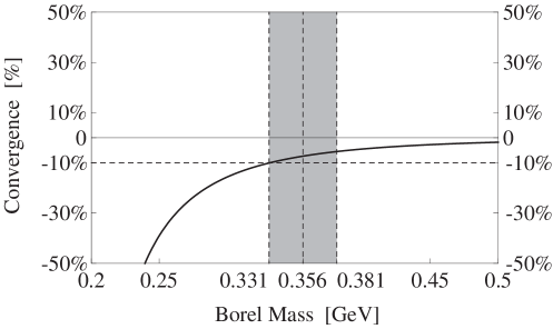
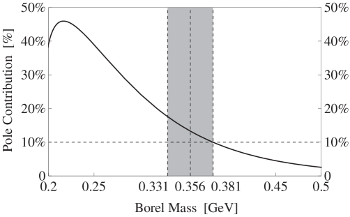
Figure 2: In the left panel we show the variation of CVG, defined in Eq. (31), as a function of the Borel mass $T$. In the right panel we show the variation of PC, defined in Eq. (33), as a function of the Borel mass $T$, where the threshold value is chosen to be $\omega_{c}$ = 2.5 GeV. The current $J^{\alpha}_{3/2,+,\Lambda_{c},2,0,\lambda\lambda}$ is used here.

Figure 3: The variations of $\overline{\Lambda}_{\Lambda_{c},2,0,\lambda\lambda}$ (left) and $f_{\Lambda_{c},2,0,\lambda\lambda}$ (right) with respect to the Borel mass $T$, when $J^{\alpha}_{3/2,+,\Lambda_{c},2,0,\lambda\lambda}$ is used. The short-dashed, solid, and long-dashed curves are obtained by fixing $\omega_{c}=2.3$, 2.5, and 2.7 GeV, respectively.

Still using the current $J^{\alpha}_{3/2,+,\Lambda_{c},2,0,\lambda\lambda}$ as an example, we show the variations of CVG and PC, as defined in Eqs. (31) and (33), with respect to the Borel mass $T$ in Fig. 2, and the variations of $\overline{\Lambda}_{\Lambda_{c},2,0,\lambda\lambda}$ and $f_{\Lambda_{c},2,0,\lambda\lambda}$ with respect to $T$ in Fig. 3, where $\omega_{c}$ is chosen to be 2.5 GeV. Now the Borel window is $0.331$ GeV $<T<0.381$ GeV, and we obtain the following numerical results:

$$\overline{\Lambda}_{\Lambda_{c},2,0,\lambda\lambda} = 1.113\mbox{ GeV}\,,$$ (34)

$$f_{\Lambda_{c},2,0,\lambda\lambda} = 0.012\mbox{ GeV}^{5}\,,$$

where the central values are obtained by choosing $T=0.356$ GeV and $\omega_{c}=2.5$ GeV.

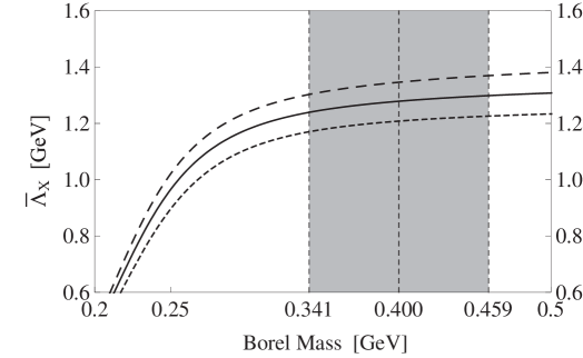
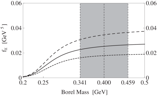
Figure 4: The variations of $\overline{\Lambda}_{\Xi_{c},2,0,\lambda\lambda}$ (left) and $f_{\Xi_{c},2,0,\lambda\lambda}$ (right) with respect to the Borel mass $T$, when $J^{\alpha}_{3/2,+,\Xi_{c},2,0,\lambda\lambda}$ is used. The short-dashed, solid, and long-dashed curves are obtained by fixing $\omega_{c}=2.8$, 3.0, and 3.2 GeV, respectively.

We also show the variations of $\overline{\Lambda}_{\Xi_{c},2,0,\lambda\lambda}$ and $f_{\Xi_{c},2,0,\lambda\lambda}$ with respect to $T$ in Fig. 4, where $\omega_{c}$ is chosen to be 3.0 GeV. From these figures, we find the Borel window $0.341$ GeV $<T<0.459$ GeV, and obtain the following numerical results:

$$\overline{\Lambda}_{\Xi_{c},2,0,\lambda\lambda} = 1.279\mbox{ GeV}\,,$$ (35)

$$f_{\Xi_{c},2,0,\lambda\lambda} = 0.025\mbox{ GeV}^{5}\,,$$

where the central values are obtained by choosing $T=0.400$ GeV and $\omega_{c}=3.0$ GeV.

IV Sum Rules at the Order ${\mathcal{O}}(1/m_{Q})$

In this section we work up to the order ${\mathcal{O}}(1/m_{Q})$ based on the HQET Lagrangian Dai:1996qx ; Dai:2003yg :

$$\mathcal{L}_{\rm eff}=\overline{h}_{v}iv\cdot Dh_{v}+\frac{1}{2m_{Q}}\mathcal{K}+\frac{1}{2m_{Q}}\mathcal{S}\,,$$ (36)

where $\mathcal{K}$ is the operator of nonrelativistic kinetic energy, and $\mathcal{S}$ is the Pauli term describing the chromomagnetic interaction:

$$\mathcal{K} = \overline{h}_{v}(iD_{t})^{2}h_{v}\,,$$ (37)

$$\mathcal{S} = \frac{g}{2}C_{mag}(m_{Q}/\mu)\overline{h}_{v}\sigma_{\mu\nu}G^{\mu\nu}h_{v}\,.$$

Here $C_{mag}(m_{Q}/\mu)=[\alpha_{s}(m_{Q})/\alpha_{s}(\mu)]^{3/\beta_{0}}$ with $\beta_{0}=11-2n_{f}/3$.

The correlation function at the hadron level, Eq. (24), can be written up to the order ${\mathcal{O}}(1/m_{Q})$ as

$$\Pi(\omega)_{pole} = \frac{2(f+\delta f)^{2}}{2(\overline{\Lambda}+\delta m)-\omega}$$

$$= \frac{2f^{2}}{2\overline{\Lambda}-\omega}-\frac{4\delta mf^{2}}{(2\overline{\Lambda}-\omega)^{2}}+\frac{4f\delta f}{2\overline{\Lambda}-\omega}\,,$$

where $\delta m_{j,P,F,j_{l},s_{l},\rho\rho/\lambda\lambda/\rho\lambda}$ is the correction to the mass $m_{j,P,F,j_{l},s_{l},\rho\rho/\lambda\lambda/\rho\lambda}$, and can be evaluated using the three-point correlation functions:

$$\delta_{O}\Pi_{j,P,F,j_{l},s_{l},\rho\rho/\lambda\lambda/\rho\lambda}^{\alpha_{1}\cdots\alpha_{j-1/2},\beta_{1}\cdots\beta_{j-1/2}}(\omega,\omega^{\prime}) = i^{2}\int d^{4}xd^{4}ye^{ik\cdot x-ik^{\prime}\cdot y}\times\langle 0|T[J_{j,P,F,j_{l},s_{l},\rho\rho/\lambda\lambda/\rho\lambda}^{\alpha_{1}\cdots\alpha_{j-1/2}}(x)O(0)\bar{J}_{j,P,F,j_{l},s_{l},\rho\rho/\lambda\lambda/\rho\lambda}^{\beta_{1}\cdots\beta_{j-1/2}}(y)]|0\rangle$$ (39)

$$= \mathbb{S}[g_{t}^{\alpha_{1}\beta_{1}}\cdots g_{t}^{\alpha_{j-1/2}\beta_{j-1/2}}]\delta_{O}\Pi_{j,P,F,j_{l},s_{l},\rho\rho/\lambda\lambda/\rho\lambda}(\omega)\,,$$

where $O=\mathcal{K}$ or $\mathcal{S}$. Based on the Lagrangian (36), these correlation functions can be written at the hadron level as

$$\delta_{\mathcal{K}}\Pi(\omega,\omega^{\prime})_{j,P,F,j_{l},s_{l},\rho\rho/\lambda\lambda/\rho\lambda} = \frac{2f^{2}K_{F,j_{l},s_{l},\rho\rho/\lambda\lambda/\rho\lambda}}{(2\overline{\Lambda}-\omega)(2\overline{\Lambda}-\omega^{\prime})}+\frac{2f^{2}G_{\mathcal{K}}(\omega^{\prime})}{2\overline{\Lambda}-\omega}+\frac{2f^{2}G_{\mathcal{K}}(\omega)}{2\overline{\Lambda}-\omega^{\prime}}\,,$$ (40)

$$\delta_{\mathcal{S}}\Pi(\omega,\omega^{\prime})_{j,P,F,j_{l},s_{l},\rho\rho/\lambda\lambda/\rho\lambda} = \frac{2d_{M}f^{2}\Sigma_{F,j_{l},s_{l},\rho\rho/\lambda\lambda/\rho\lambda}}{(2\overline{\Lambda}-\omega)(2\overline{\Lambda}-\omega^{\prime})}+\frac{2d_{M}f^{2}G_{\mathcal{S}}(\omega^{\prime})}{2\overline{\Lambda}-\omega}\,+\frac{2d_{M}f^{2}G_{\mathcal{S}}(\omega)}{2\overline{\Lambda}-\omega^{\prime}}\,,$$ (41)

where the following definitions have been used:

$$K_{F,j_{l},s_{l},\rho\rho/\lambda\lambda/\rho\lambda} \equiv \langle j,P,F,j_{l},s_{l},\rho\rho/\lambda\lambda/\rho\lambda|\overline{h}_{v}(iD_{\bot})^{2}h_{v}|j,P,F,j_{l},s_{l},\rho\rho/\lambda\lambda/\rho\lambda\rangle\,,$$

$$d_{M}\Sigma_{F,j_{l},s_{l},\rho\rho/\lambda\lambda/\rho\lambda} \equiv \langle j,P,F,j_{l},s_{l},\rho\rho/\lambda\lambda/\rho\lambda|{g\over 2}\overline{h}_{v}\sigma_{\mu\nu}G^{\mu\nu}h_{v}|j,P,F,j_{l},s_{l},\rho\rho/\lambda\lambda/\rho\lambda\rangle\,,$$

$$d_{M} \equiv d_{j,j_{l}}\,,$$ (42)

$$d_{j_{l}-1/2,j_{l}} = 2j_{l}+2\,,$$

$$d_{j_{l}+1/2,j_{l}} = -2j_{l}\,.$$

Then we fix $\omega=\omega^{\prime}$ and use Eqs. (IV), (40), and (41) to obtain

$$\delta m_{j,P,F,j_{l},s_{l},\rho\rho/\lambda\lambda/\rho\lambda}=-\frac{1}{4m_{Q}}(K_{F,j_{l},s_{l},\rho\rho/\lambda\lambda/\rho\lambda}+d_{M}C_{mag}\Sigma_{F,j_{l},s_{l},\rho\rho/\lambda\lambda/\rho\lambda})\,.$$ (43)

From this equation we find that only the term $\mathcal{S}$ ($\Sigma_{F,j_{l},s_{l},\rho\rho/\lambda\lambda/\rho\lambda}$) can cause a mass splitting within the same doublet.

The three-point correlation functions defined in Eq. (39) can also be evaluated at the quark and gluon level using the method of operator product expansion Dai:1996qx ; Dai:2003yg . Still using the currents $J^{\alpha}_{3/2,+,\Lambda_{c},2,0,\lambda\lambda}$ and $J^{\alpha}_{3/2,+,\Xi_{c},2,0,\lambda\lambda}$ as examples, we insert Eqs. (II) and (II) into Eqs. (39), make a double Borel transformation for both $\omega$ and $\omega^{\prime}$, take the two Borel parameters to be equal, and then obtain:

$$f_{\Lambda_{c},2,0,\lambda\lambda}^{2}K_{\Lambda_{c},2,0,\lambda\lambda}e^{-2\bar{\Lambda}_{\Lambda_{c},2,0,\lambda\lambda}/T}=\int_{0}^{\omega_{c}}[-\frac{127}{10644480\pi^{4}}\omega^{11}-\frac{\langle g_{s}^{2}GG\rangle}{17280\pi^{4}}\omega^{7}]e^{-\omega/T}d\omega\,,$$ (46)

$$f_{\Lambda_{c},2,0,\lambda\lambda}^{2}\Sigma_{\Lambda_{c},2,0,\lambda\lambda}e^{-2\bar{\Lambda}_{\Lambda_{c},2,0,\lambda\lambda}/T}=\int_{0}^{\omega_{c}}[\frac{\langle g_{s}^{2}GG\rangle}{24192\pi^{4}}\omega^{7}]e^{-\omega/T}d\omega\,,$$

$$f_{\Xi_{c},2,0,\lambda\lambda}^{2}K_{\Xi_{c},2,0,\lambda\lambda}e^{-2\bar{\Lambda}_{\Xi_{c},2,0,\lambda\lambda}/T}$$

$$=\int_{2m_{s}}^{\omega_{c}}[-\frac{127}{10644480\pi^{4}}\omega^{11}+\frac{307m_{s}^{2}}{483840\pi^{4}}\omega^{9}+\frac{37m_{s}\langle\bar{q}q\rangle}{5040\pi^{2}}\omega^{7}-\frac{233m_{s}\langle\bar{s}s\rangle}{20160\pi^{2}}\omega^{7}$$

$$~{}~{}~{}~{}-\frac{\langle g_{s}^{2}GG\rangle}{17280\pi^{4}}\omega^{7}-\frac{1019m_{s}^{2}\langle g_{s}^{2}GG\rangle}{184320\pi^{4}}\omega^{5}-\frac{13m_{s}\langle g_{s}^{2}GG\rangle\langle\bar{q}q\rangle}{648\pi^{2}}\omega^{3}+\frac{67m_{s}\langle g_{s}^{2}GG\rangle\langle\bar{s}s\rangle}{2304\pi^{2}}\omega^{3}]e^{-\omega/T}d\omega\,,$$ (47)

$$f_{\Xi_{c},2,0,\lambda\lambda}^{2}\Sigma_{\Xi_{c},2,0,\lambda\lambda}e^{-2\bar{\Lambda}_{\Xi_{c},2,0,\lambda\lambda}/T}$$

$$=\int_{2m_{s}}^{\omega_{c}}[\frac{\langle g_{s}^{2}GG\rangle}{24192\pi^{4}}\omega^{7}-\frac{m_{s}^{2}\langle g_{s}^{2}GG\rangle}{1536\pi^{4}}\omega^{5}+\frac{5m_{s}\langle g_{s}^{2}GG\rangle\langle\bar{s}s\rangle}{864\pi^{2}}\omega^{3}]e^{-\omega/T}d\omega\,,$$

Sum rules for other currents are shown in Appendix B.

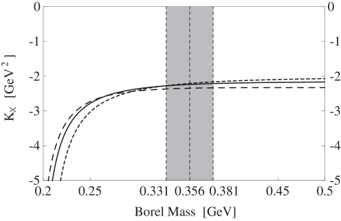
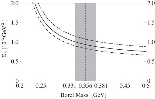
Figure 5: The variations of $K_{\Lambda_{c},2,0,\lambda\lambda}$ (left) and $\Sigma_{\Lambda_{c},2,0,\lambda\lambda}$ (right) with respect to the Borel mass $T$, when $J^{\alpha}_{3/2,+,\Lambda_{c},2,0,\lambda\lambda}$ is used. The short-dashed, solid and long-dashed curves are obtained by fixing $\omega_{c}=2.3$, 2.5 and 2.7 GeV, respectively.

Finally, we obtain $K_{\Lambda_{c},2,0,\lambda\lambda}$ and $\Sigma_{\Lambda_{c},2,0,\lambda\lambda}$ by simply dividing Eqs. (46) and (46) by Eq. (26). Their variations are shown in Fig. 5 with respect to the Borel mass $T$. We find their dependence on $T$ is weak in the Borel window $0.331$ GeV $<T<0.381$ GeV, and obtain the following numerical results:

$$K_{\Lambda_{c},2,0,\lambda\lambda} = -2.239\mbox{ GeV}^{2}\,,$$ (48)

$$\Sigma_{\Lambda_{c},2,0,\lambda\lambda} = 0.014\mbox{ GeV}^{2}\,,$$

where the central values are obtained by choosing $T=0.356$ GeV and $\omega_{c}=2.5$ GeV.

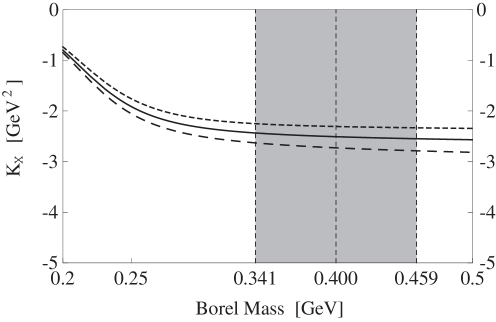
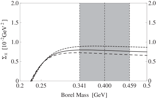
Figure 6: The variations of $K_{\Xi_{c},2,0,\lambda\lambda}$ (left) and $\Sigma_{\Xi_{c},2,0,\lambda\lambda}$ (right) with respect to the Borel mass $T$, when $J^{\alpha}_{3/2,+,\Xi_{c},2,0,\lambda\lambda}$ is used. The short-dashed, solid and long-dashed curves are obtained by fixing $\omega_{c}=2.8$, 3.0 and 3.2 GeV, respectively.

We also obtain $K_{\Xi_{c},2,0,\lambda\lambda}$ and $\Sigma_{\Xi_{c},2,0,\lambda\lambda}$ by simply dividing Eqs. (46) and (47) by Eq. (III), and show their variations in Fig. 6 with respect to the Borel mass $T$. We find their dependence on $T$ is weak in the Borel window $0.341$ GeV $<T<0.459$ GeV, and obtain the following numerical results:

$$K_{\Xi_{c},2,0,\lambda\lambda} = -2.508\mbox{ GeV}^{2}\,,$$ (49)

$$\Sigma_{\Xi_{c},2,0,\lambda\lambda} = 0.008\mbox{ GeV}^{2}\,,$$

where the central values are obtained by choosing $T=0.400$ GeV and $\omega_{c}=3.0$ GeV.

V Numerical Results and Discussions

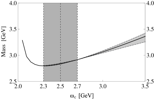
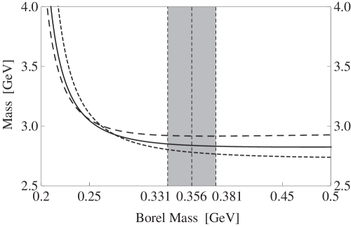
Figure 7: Variations of $m_{\Lambda_{c}(5/2^{+})}$ with respect to the threshold value $\omega_{c}$ (left) and the Borel mass $T$ (right), calculated using the charmed baryon doublet $[\Lambda_{c},2,0,\lambda\lambda]$. In the left panel, the shady band is obtained by changing $T$ inside Borel windows. The mass curves have minimum against $\omega_{c}$ around 2.2 GeV, where the $\omega_{c}$ dependence of the mass prediction is the weakest. However, at this point there does not exist any non-vanishing working region of the Borel mass $T$. We find that there exist non-vanishing working regions of $T$ as long as $\omega_{c}\geq 2.3$ GeV, and the $\omega_{c}$ dependence is still weak and acceptable in the region $2.3$ GeV$<\omega_{c}<2.7$ GeV. The results for $\omega_{c}<2.3$ GeV are also shown, for which cases we choose the Borel mass $T$ when the PC, as defined in Eq. (34), is around 10%. In the right figure, the short-dashed, solid and long-dashed curves are obtained by fixing $\omega_{c}=2.3$, 2.5 and 2.7 GeV, respectively.

Combining the results obtained in Sec. III and Sec. IV, we obtain the masses of the heavy baryon doublet $[\Lambda_{c},2,0,\lambda\lambda]$ satisfying:

$$m_{\Lambda_{c}({3/2}^{+})} = m_{c}+\overline{\Lambda}_{\Lambda_{c},2,0,\lambda\lambda}-{1\over 4m_{c}}[K_{\Lambda_{c},2,0,\lambda\lambda}+d_{3/2,2}\Sigma_{\Lambda_{c},2,0,\lambda\lambda}]\,,$$ (50)

$$m_{\Lambda_{c}({5/2}^{+})} = m_{c}+\overline{\Lambda}_{\Lambda_{c},2,0,\lambda\lambda}-{1\over 4m_{c}}[K_{\Lambda_{c},2,0,\lambda\lambda}+d_{5/2,2}\Sigma_{\Lambda_{c},2,0,\lambda\lambda}]\,.$$

After inserting $d_{3/2,2}=6$ and $d_{5/2,2}=-4$, we arrive at:

$${1\over 10}\Big{(}4m_{\Lambda_{c}({3/2}^{+})}+6m_{\Lambda_{c}({5/2}^{+})}\Big{)} = m_{c}+1.113\mbox{ GeV }-{1\over 4m_{c}}[-2.239\mbox{ GeV}^{2}]\,,$$ (51)

$$m_{\Lambda_{c}({5/2}^{+})}-m_{\Lambda_{c}({3/2}^{+})} = {1\over 4m_{c}}\times{10}\times[0.014\mbox{ GeV}^{2}]\,,$$

where $\Lambda_{c}({3/2}^{+})$ and $\Lambda_{c}({5/2}^{+})$ are the two baryons contained in this doublet. Clearly, the $\mathcal{O}(1/m_{Q})$ corrections can not be neglected. Then we use the PDG value $m_{c}=1.275\pm 0.025$ GeV pdg for the charm quark mass in the $\overline{\rm MS}$ scheme to obtain numerical results:

$$m_{\Lambda_{c}({3/2}^{+})} = 2.81\mbox{ GeV}\,,$$

$$m_{\Lambda_{c}({5/2}^{+})} = 2.84\mbox{ GeV}\,,$$ (52)

$$m_{\Lambda_{c}({5/2}^{+})}-m_{\Lambda_{c}({3/2}^{+})} = 28\mbox{ MeV}\,.$$

These values are obtained for $\omega_{c}=2.5$ GeV. We change the threshold value $\omega_{c}$ and redo the same procedures. We note that our third criterion is to require the dependence of $m_{j,P,F,j_{l},s_{l},\rho\rho/\lambda\lambda/\rho\lambda}$ (mass of the heavy baryon state) on this parameter $\omega_{c}$ to be weak. Accordingly, we show the variation of $m_{\Lambda_{c}(5/2^{+})}$ with respect to $\omega_{c}$ in the left panel of Fig. 7 in a large region 2.0 GeV$<\omega_{c}<3.5$ GeV. The mass curves have minimum against $\omega_{c}$ around 2.2 GeV, where the $\omega_{c}$ dependence of the mass prediction is the weakest. However, at this point we apply the two criteria on the Borel mass $T$ (see discussions in Sec. III) but can not obtain any non-vanishing working region of $T$. We find that there exist non-vanishing working regions of $T$ as long as $\omega_{c}\geq 2.3$ GeV, and the $\omega_{c}$ dependence is still weak and acceptable in the region $2.3$ GeV$<\omega_{c}<2.7$ GeV. Hence, we choose $2.3$ GeV$<\omega_{c}<2.7$ GeV and $0.331$ GeV $<T<0.381$ GeV as our working regions, and obtain the following numerical results for the baryon doublet $[\Lambda_{c},2,0,\lambda\lambda]$:

$$m_{\Lambda_{c}({3/2}^{+})} = 2.81^{+0.33}_{-0.18}\mbox{ GeV}\,,$$

$$m_{\Lambda_{c}({5/2}^{+})} = 2.84^{+0.37}_{-0.20}\mbox{ GeV}\,,$$ (53)

$$m_{\Lambda_{c}({5/2}^{+})}-m_{\Lambda_{c}({3/2}^{+})} = 28^{+45}_{-24}\mbox{ MeV}\,,$$

whose central values correspond to $T=0.356$ GeV and $\omega_{c}=2.5$ GeV, and the uncertainties are due to the Borel mass $T$, the threshold value $\omega_{c}$, the charm quark mass $m_{c}$ and the quark and gluon condensates. We also show the variation of $m_{\Lambda_{c}(5/2^{+})}$ with respect to the Borel mass $T$ in the right panel of Fig. 7, in a broad region $0.2$ GeV$<T<0.5$ GeV, where these curves are more stable inside the Borel window $0.331$ GeV $<T<0.381$ GeV. The mass of the $\Lambda_{c}({5/2}^{+})$ in the doublet $[\Lambda_{c},2,0,\lambda\lambda]$ is consistent with the mass of the $\Lambda_{c}(2880)$ pdg :

$$m^{\rm exp}_{\Lambda_{c}(2880),5/2^{+}}=2881.53\pm 0.35\mbox{ MeV}\,,$$ (54)

and supports it to be a $D$-wave charmed baryon of $J^{P}=5/2^{+}$. Our result further suggests that the $\Lambda_{c}(2880)$ of $J^{P}=5/2^{+}$ has a partner state, the $\Lambda_{c}(3/2^{+})$ of $J^{P}=3/2^{+}$. Its mass is $2.81^{+0.33}_{-0.18}$ GeV, and the mass difference between it and the $\Lambda_{c}(2880)$ is $28^{+45}_{-24}$ MeV. We note that there are large theoretical uncertainties in our results for the masses of the heavy baryons, but their differences within the same doublet are produced with much less theoretical uncertainty because they do not depend much on the charm quark mass and the threshold value Chen:2015kpa ; Mao:2015gya .

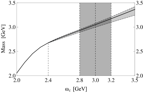
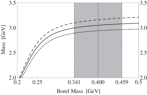
Figure 8: Variations of $m_{\Xi_{c}(5/2^{+})}$ with respect to the threshold value $\omega_{c}$ (left) and the Borel mass $T$ (right), calculated using the charmed baryon doublet $[\Xi_{c},2,0,\lambda\lambda]$. In the left panel, the shady band is obtained by changing $T$ inside Borel windows, which exist as long as $\omega_{c}\geq 2.4$ GeV. We properly fine-tune the threshold value $\omega_{c}$ to be around 3.0 GeV so that $\omega_{c}(\Xi_{c}(5/2^{+}))-\omega_{c}(\Lambda_{c}(5/2^{+}))=0.5$ GeV, which value is the same as those used in our previous studies on $P$-wave heavy baryons Chen:2015kpa ; Mao:2015gya . In the right figure, the short-dashed, solid and long-dashed curves are obtained by fixing $\omega_{c}=2.8$, 3.0 and 3.2 GeV, respectively.

We follow the same procedures to study the baryon doublet $[\Xi_{c},2,0,\lambda\lambda]$, and show the variation of $m_{\Xi_{c}(5/2^{+})}$ with respect to the threshold value $\omega_{c}$ in the left panel of Fig. 8. Different from the case of $m_{\Lambda_{c}(5/2^{+})}$, the mass curves do not have minimum against $\omega_{c}$, but the $\omega_{c}$ dependence of the mass prediction is still not strong when $\omega_{c}>2.5$ GeV where there exist Borel windows. We properly fine-tune the threshold value $\omega_{c}$ to be around 3.0 GeV so that $\omega_{c}(\Xi_{c}(5/2^{+}))-\omega_{c}(\Lambda_{c}(5/2^{+}))=0.5$ GeV, which value is the same as those used in our previous studies on $P$-wave heavy baryons Chen:2015kpa ; Mao:2015gya . Together we choose $2.8$ GeV$<\omega_{c}<3.2$ GeV and $0.341$ GeV $<T<0.459$ GeV as our working regions, and obtain the following numerical results for the baryon doublet $[\Xi_{c},2,0,\lambda\lambda]$:

$$m_{\Xi_{c}({3/2}^{+})} = 3.04^{+0.15}_{-0.15}\mbox{ GeV}\,,$$

$$m_{\Xi_{c}({5/2}^{+})} = 3.05^{+0.15}_{-0.16}\mbox{ GeV}\,,$$ (55)

$$m_{\Xi_{c}({5/2}^{+})}-m_{\Xi_{c}({3/2}^{+})} = 15^{+16}_{-13}\mbox{ MeV}\,,$$

whose central values correspond to $T=0.400$ GeV and $\omega_{c}=3.0$ GeV. We also show the variation of $m_{\Xi_{c}(5/2^{+})}$ with respect to the Borel mass $T$ in the right panel of Fig. 8, where these curves are stable inside the Borel window $0.341$ GeV $<T<0.459$ GeV. The masses of the $\Xi_{c}({3/2}^{+})$ and $\Xi_{c}({5/2}^{+})$ in the doublet $[\Xi_{c},2,0,\lambda\lambda]$ are consistent with the masses of the $\Xi_{c}(3055)$ and $\Xi_{c}(3080)$ pdg as well as their difference:

$$m^{\rm exp}_{\Xi_{c}(3055)^{+}}=3055.1\pm 1.7\mbox{ MeV}\,,$$

$$m^{\rm exp}_{\Xi_{c}(3080)^{+}}=3076.94\pm 0.28\mbox{ MeV}\,,m^{\rm exp}_{\Xi_{c}(3080)^{0}}=3079.9\pm 1.4\mbox{ MeV}\,,$$ (56)

$$m^{\rm exp}_{\Xi_{c}(3080)^{+}}-m^{\rm exp}_{\Xi_{c}(3055)^{+}}=21.8\pm 1.7\mbox{ MeV}\,.$$

This suggests that the $\Xi_{c}(3055)$ and $\Xi_{c}(3080)$ have quantum number $J^{P}=3/2^{+}$ and $5/2^{+}$, respectively, which assignments have been proposed or discussed in detail in Refs. Ebert:2011kk ; Chen:2014nyo ; Cheng:2015rra .

Table 1: Masses of the $D$-wave charmed baryons obtained using the baryon doublets $[\mathbf{\bar{3}}_{F},2,0,\rho\rho]$, $[\mathbf{\bar{3}}_{F},2,0,\lambda\lambda]$, $[\mathbf{\bar{3}}_{F},1,1,\rho\lambda]$, $[\mathbf{\bar{3}}_{F},2,1,\rho\lambda]$ and $[\mathbf{\bar{3}}_{F},3,1,\rho\lambda]$. As discussed at the end of Sec. II, a) for the baryon doublet $[\mathbf{\bar{3}}_{F},3,1,\rho\lambda]$ containing $\Lambda_{c}(5/2^{+},7/2^{+})$ and $\Xi_{c}(5/2^{+},7/2^{+})$, we only evaluate their average masses ${1\over 14}(6m_{\Lambda_{c}({5/2}^{+})}+8m_{\Lambda_{c}({7/2}^{+})})$ and ${1\over 14}(6m_{\Xi_{c}({5/2}^{+})}+8m_{\Xi_{c}({7/2}^{+})})$; b) for the baryon doublet $[\mathbf{\bar{3}}_{F},2,1,\rho\lambda]$ ($s_{l}=1$ and $j_{l}=2$), we estimate their masses by simply averaging between $[\mathbf{\bar{3}}_{F},1,1,\rho\lambda]$ ($s_{l}=1$ and $j_{l}=1$) and $[\mathbf{\bar{3}}_{F},3,1,\rho\lambda]$ ($s_{l}=1$ and $j_{l}=3$). We assume that free parameters $\omega_{c}$ in the same multiplet satisfy the relation $\omega_{c}(\Xi_{c})-\omega_{c}(\Lambda_{c})=0.5$ GeV, except for the $[\mathbf{\bar{3}}_{F},1,1,\rho\lambda]$.

Multiplets	B	$\omega_{c}$	Working region	$\overline{\Lambda}$	$f$	$K$	$\Sigma$	Baryons	Mass	Difference
		(GeV)	(GeV)	(GeV)	(GeV5)	(GeV2)	(GeV2)	($j^{P}$)	(GeV)	(MeV)
$[\mathbf{\bar{3}}_{F},2,0,\lambda\lambda]$	$\Lambda_{c}$	2.5	$0.331<T<0.381$	$1.113$	$0.012$	$-2.239$	$0.014$	$\Lambda_{c}(3/2^{+})$	$2.81^{+0.33}_{-0.18}$	$28^{+45}_{-24}$
								$\Lambda_{c}(5/2^{+})$	$2.84^{+0.37}_{-0.20}$
	$\Xi_{c}$	3.0	$0.341<T<0.459$	$1.279$	$0.025$	$-2.508$	$0.008$	$\Xi_{c}(3/2^{+})$	$3.04^{+0.15}_{-0.15}$	$15^{+16}_{-13}$
								$\Xi_{c}(5/2^{+})$	$3.05^{+0.15}_{-0.16}$
$[\mathbf{\bar{3}}_{F},2,0,\rho\rho]$	$\Lambda_{c}$	3.4	$0.358<T<0.499$	$1.650$	$0.065$	$-1.742$	$0.011$	$\Lambda_{c}(3/2^{+})$	$3.25^{+1.72}_{-0.28}$	$22^{+120}_{-20}$
								$\Lambda_{c}(5/2^{+})$	$3.28^{+1.83}_{-0.30}$
	$\Xi_{c}$	3.9	$0.502<T<0.591$	$1.723$	$0.10$	$-1.308$	$0.006$	$\Xi_{c}(3/2^{+})$	$3.25^{+0.16}_{-0.14}$	$11^{+16}_{-9}$
								$\Xi_{c}(5/2^{+})$	$3.26^{+0.17}_{-0.15}$
$[\mathbf{\bar{3}}_{F},1,1,\rho\lambda]$	$\Lambda_{c}$	3.0	$0.397<T<0.457$	$1.335$	$0.044$	$-2.116$	$0.006$	$\Lambda_{c}(1/2^{+})$	$3.02^{+0.19}_{-0.14}$	$7^{+11}_{-6}$
								$\Lambda_{c}(3/2^{+})$	$3.03^{+0.20}_{-0.14}$
	$\Xi_{c}$	4.0	$0.526<T<0.599$	$1.887$	$0.21$	$-2.954$	$0.003$	$\Xi_{c}(1/2^{+})$	$3.74^{+0.14}_{-0.13}$	$3^{+3}_{-3}$
								$\Xi_{c}(3/2^{+})$	$3.74^{+0.14}_{-0.13}$
$\begin{array}[]{c}[\mathbf{\bar{3}}_{F},2,1,\rho\lambda]\\ {\rm(estimated)}\end{array}$	$\Lambda_{c}$	–	–	–	–	–	–	$\Lambda_{c}(3/2^{+})$	$\sim 3.20$	–
								$\Lambda_{c}(5/2^{+})$
	$\Xi_{c}$	–	–	–	–	–	–	$\Xi_{c}(3/2^{+})$	$\sim 3.76$	–
								$\Xi_{c}(5/2^{+})$
$\begin{array}[]{c}[\mathbf{\bar{3}}_{F},3,1,\rho\lambda]\\ {\rm(simplified)}\end{array}$	$\Lambda_{c}$	3.6	$0.496<T<0.542$	$1.628$	$0.022$	$-2.939$	–	$\Lambda_{c}(5/2^{+})$	$3.48^{+0.33}_{-0.18}$	–
								$\Lambda_{c}(7/2^{+})$
	$\Xi_{c}$	4.1	$0.556<T<0.609$	$1.920$	$0.045$	$-3.105$	–	$\Xi_{c}(5/2^{+})$	$3.80^{+0.20}_{-0.16}$	–
								$\Xi_{c}(7/2^{+})$

We also study the other four baryon doublets, $[\mathbf{\bar{3}}_{F},2,0,\rho\rho]$, $[\mathbf{\bar{3}}_{F},1,1,\rho\lambda]$, $[\mathbf{\bar{3}}_{F},2,1,\rho\lambda]$ and $[\mathbf{\bar{3}}_{F},3,1,\rho\lambda]$. Two important notes are:

1. It is too complicated to directly use $J^{\alpha_{1}\alpha_{2}\alpha_{3}}_{7/2,+,\mathbf{\bar{3}}_{F},3,1,\rho\lambda}$, defined in Eq. (d), to perform QCD sum rule analyses, so we shall use its simplified version without the projection operator $\Gamma^{\alpha_{1}\alpha_{2}\alpha_{3},\mu_{1}\mu_{2}\mu_{3}}$:

   $$J^{\prime\alpha_{1}\alpha_{2}\alpha_{3}}_{7/2,+,\mathbf{\bar{3}}_{F},3,1,\rho\lambda}(x) = \mathbb{S}^{\prime}[i^{2}\epsilon_{abc}\Big{(}[\mathcal{D}^{\alpha_{1}}\mathcal{D}^{\alpha_{2}}q^{aT}(x)]\mathbb{C}\gamma_{\alpha_{3}}q^{b}(x)-q^{aT}(x)\mathbb{C}\gamma_{\alpha_{3}}[\mathcal{D}^{\alpha_{1}}\mathcal{D}^{\alpha_{2}}q^{b}(x)]\Big{)}\times h_{v}^{c}(x)]\,,$$ (57)

   where $\mathbb{S}^{\prime}[\cdots]$ is used to denote symmetrization and subtracting the trace terms in the sets $(\alpha_{1}\cdots\alpha_{3})$. Using this current, we can well calculate sum rules at the leading order as well as the $\mathcal{K}$ correction ($K_{\mathbf{\bar{3}}_{F},3,1,\rho\lambda}$) at the order ${\mathcal{O}}(1/m_{Q})$, but the $\mathcal{S}$ correction ($\Sigma_{\mathbf{\bar{3}}_{F},3,1,\rho\lambda}$) at the order ${\mathcal{O}}(1/m_{Q})$ can not be evaluated.

2. Because we failed to construct the two currents belonging to the baryon doublet $[\mathbf{\bar{3}}_{F},2,1,\rho\lambda]$ with $s_{l}=1$ and $j_{l}=2$, we shall estimate their masses by averaging between $[\mathbf{\bar{3}}_{F},1,1,\rho\lambda]$ ($s_{l}=1$ and $j_{l}=1$) and $[\mathbf{\bar{3}}_{F},3,1,\rho\lambda]$ ($s_{l}=1$ and $j_{l}=3$), weighted by the spin-orbital splittings:

   $$l_{\rho}\otimes s_{l}={1\over 2}\big{(}j_{l}(j_{l}+1)-l_{\rho}(l_{\rho}+1)-s_{l}(s_{l}+1)\big{)}={1\over 2}\big{(}j_{l}(j_{l}+1)-4\big{)}\,.$$ (58)

   Hence, we obtain

   $${\rm Mass}(j_{l}=2)={3\over 5}\times{\rm Mass}(j_{l}=1)+{2\over 5}\times{\rm Mass}(j_{l}=3)\,.$$ (59)

However, their obtained results are difficult to explain the $\Lambda_{c}(2880)$, $\Xi_{c}(3055)$ and $\Xi_{c}(3080)$ at the same time:

1. The baryon doublet $[\mathbf{\bar{3}}_{F},2,0,\rho\rho]$ contains $\Lambda_{c}(3/2^{+},5/2^{+})$ and $\Xi_{c}(3/2^{+},5/2^{+})$. We use them to perform QCD sum rule analyses, and show variations of $m_{\Lambda_{c}(5/2^{+})}$ and $m_{\Xi_{c}(5/2^{+})}$ with respect to the threshold value $\omega_{c}$ in Fig. 9. The obtained masses are listed in Table 1:

   $$m_{\Lambda_{c}({3/2}^{+})} = 3.25^{+1.72}_{-0.28}\mbox{ GeV}\,,m_{\Lambda_{c}({5/2}^{+})}=3.28^{+1.83}_{-0.30}\mbox{ GeV}\,,\Delta m=22^{+120}_{-20}\mbox{ MeV}\,,$$ (60)

   $$m_{\Xi_{c}({3/2}^{+})} = 3.25^{+0.16}_{-0.14}\mbox{ GeV}\,,m_{\Xi_{c}({5/2}^{+})}=3.26^{+0.17}_{-0.15}\mbox{ GeV}\,,\Delta m=11^{+16}_{-9}\mbox{ MeV}\,,$$

   whose values are significantly larger than the masses of the $\Lambda_{c}(2880)$, $\Xi_{c}(3055)$ and $\Xi_{c}(3080)$.

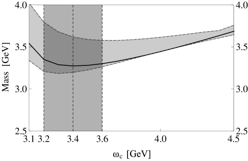
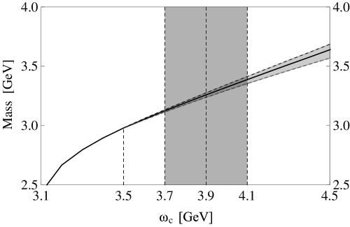
   Figure 9: Variations of $m_{\Lambda_{c}(5/2^{+})}$ (left) and $m_{\Xi_{c}(5/2^{+})}$ (right) with respect to the threshold value $\omega_{c}$, calculated using the charmed baryon doublet $[\mathbf{\bar{3}}_{F},2,0,\rho\rho]$. The shady band is obtained by changing $T$ inside Borel windows, which exist as long as $\omega_{c}\geq 3.1$ GeV (left) and $\omega_{c}\geq 3.5$ GeV (right). In the left panel we choose $\omega_{c}$ to be around 3.4 GeV, where the mass curves have minimum against it. In the right panel we properly fine-tune $\omega_{c}$ to be around 3.9 GeV so that $\omega_{c}(\Xi_{c}(5/2^{+}))-\omega_{c}(\Lambda_{c}(5/2^{+}))=0.5$ GeV.

2. The baryon doublet $[\mathbf{\bar{3}}_{F},1,1,\rho\lambda]$ contains $\Lambda_{c}(1/2^{+},3/2^{+})$ and $\Xi_{c}(1/2^{+},3/2^{+})$. This doublet does not contain any baryon of $J^{P}=5/2^{+}$. We use them to perform QCD sum rule analyses, and show variations of $m_{\Lambda_{c}(3/2^{+})}$ and $m_{\Xi_{c}(3/2^{+})}$ with respect to the threshold value $\omega_{c}$ in Fig. 10. The obtained masses are listed in Table 1:

   $$m_{\Lambda_{c}({1/2}^{+})} = 3.02^{+0.19}_{-0.14}\mbox{ GeV}\,,m_{\Lambda_{c}({3/2}^{+})}=3.03^{+0.20}_{-0.14}\mbox{ GeV}\,,\Delta m=7^{+11}_{-6}\mbox{ MeV}\,,$$ (61)

   $$m_{\Xi_{c}({1/2}^{+})} = 3.74^{+0.14}_{-0.13}\mbox{ GeV}\,,m_{\Xi_{c}({3/2}^{+})}=3.74^{+0.14}_{-0.13}\mbox{ GeV}\,,\Delta m=3^{+3}_{-3}\mbox{ MeV}\,.$$

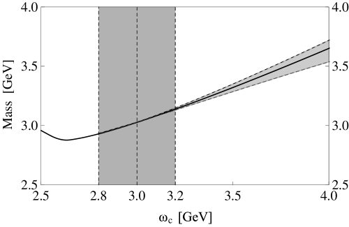
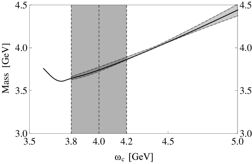
   Figure 10: Variations of $m_{\Lambda_{c}(3/2^{+})}$ (left) and $m_{\Xi_{c}(3/2^{+})}$ (right) with respect to the threshold value $\omega_{c}$, calculated using the charmed baryon doublet $[\mathbf{\bar{3}}_{F},1,1,\rho\lambda]$. The shady band is obtained by changing $T$ inside Borel windows. Although the mass curves have minimum against $\omega_{c}$ around 2.6 GeV (left) and 3.7 GeV (right), there exist Borel windows as long as $\omega_{c}\geq 2.8$ GeV (left) and $\omega_{c}\geq 3.8$ GeV (right), and the $\omega_{c}$ dependence is still weak and acceptable in the region 2.8 GeV $<\omega_{c}<$ 3.2 GeV (left) and 3.8 GeV $<\omega_{c}<$ 4.2 GeV (right).

3. The baryon doublet $[\mathbf{\bar{3}}_{F},3,1,\rho\lambda]$ contains $\Lambda_{c}(5/2^{+},7/2^{+})$ and $\Xi_{c}(5/2^{+},7/2^{+})$. We use them to perform QCD sum rule analyses. As discussed at the end of Sec. II, we can only calculate their average masses. Using the following formulae

   $$m_{\Lambda_{c}({5/2}^{+})} = m_{c}+\overline{\Lambda}_{\Lambda_{c},3,1,\rho\lambda}-{1\over 4m_{c}}[K_{\Lambda_{c},3,1,\rho\lambda}+d_{5/2,3}\Sigma_{\Lambda_{c},3,1,\rho\lambda}]\,,$$ (62)

   $$m_{\Lambda_{c}({7/2}^{+})} = m_{c}+\overline{\Lambda}_{\Lambda_{c},3,1,\rho\lambda}-{1\over 4m_{c}}[K_{\Lambda_{c},3,1,\rho\lambda}+d_{7/2,3}\Sigma_{\Lambda_{c},3,1,\rho\lambda}]\,,$$

   and similar formulae for the $\Xi_{c}({5/2}^{+})$ and $\Xi_{c}({7/2}^{+})$, we can obtain

   $${1\over 14}\Big{(}6m_{\Lambda_{c}({5/2}^{+})}+8m_{\Lambda_{c}({7/2}^{+})}\Big{)} = 3.48^{+0.33}_{-0.18}\mbox{ GeV }\,,$$ (63)

   $${1\over 14}\Big{(}6m_{\Xi_{c}({5/2}^{+})}+8m_{\Xi_{c}({7/2}^{+})}\Big{)} = 3.80^{+0.20}_{-0.16}\mbox{ GeV }\,.$$

   These values are listed in Table 1, which are significantly larger than the masses of the $\Lambda_{c}(2880)$, $\Xi_{c}(3055)$ and $\Xi_{c}(3080)$. We also show their variations with respect to the threshold value $\omega_{c}$ in Fig. 11.

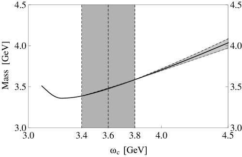
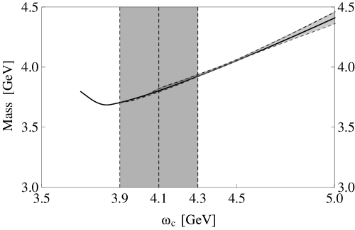
   Figure 11: Variations of $m_{[\Lambda_{c},3,1,\rho\lambda]}$ (left) and $m_{[\Xi_{c},3,1,\rho\lambda]}$ (right) with respect to the threshold value $\omega_{c}$, calculated using the charmed baryon doublet $[\mathbf{\bar{3}}_{F},3,1,\rho\lambda]$. The shady band is obtained by changing $T$ inside Borel windows. Although the mass curves have minimum against $\omega_{c}$ around 3.2 GeV (left) and 3.8 GeV (right), there exist Borel windows as long as $\omega_{c}\geq 3.4$ GeV (left) and $\omega_{c}\geq 3.9$ GeV (right), and the $\omega_{c}$ dependence is still weak and acceptable in the region 3.4 GeV $<\omega_{c}<$ 3.8 GeV (left) and 3.9 GeV $<\omega_{c}<$ 4.3 GeV (right). Moreover, these two threshold values satisfy $\omega_{c}(\Xi_{c})-\omega_{c}(\Lambda_{c})=0.5$ GeV.

4. The baryon doublet $[\mathbf{\bar{3}}_{F},2,1,\rho\lambda]$ contains $\Lambda_{c}(3/2^{+},5/2^{+})$ and $\Xi_{c}(3/2^{+},5/2^{+})$. We estimate their masses by averaging between $[\mathbf{\bar{3}}_{F},1,1,\rho\lambda]$ ($s_{l}=1$ and $j_{l}=1$) and $[\mathbf{\bar{3}}_{F},3,1,\rho\lambda]$ ($s_{l}=1$ and $j_{l}=3$), weighted by the spin-orbital splittings, to be:

   $$m_{[\Lambda_{c},2,1,\rho\lambda]} \sim 3.20\mbox{ GeV }\,,$$ (64)

   $$m_{[\Xi_{c},2,1,\rho\lambda]} \sim 3.76\mbox{ GeV }\,,$$

   These values are listed in Table 1, which are significantly larger than the masses of the $\Lambda_{c}(2880)$, $\Xi_{c}(3055)$ and $\Xi_{c}(3080)$.

VI Summary

Summarizing all these results, we have studied the $D$-wave charmed baryons of $SU(3)$ flavor $\mathbf{\bar{3}}_{F}$ using the method of QCD sum rules within HQET. We have calculated their masses up to the order $\mathcal{O}(1/m_{Q})$ with large theoretical uncertainty, and we have also calculated their mass splittings within the same doublet with much less theoretical uncertainty. Our results suggest that the $\Lambda_{c}(2880)$, $\Xi_{c}(3055)$ and $\Xi_{c}(3080)$ can be well described by the baryon doublet $[\mathbf{\bar{3}}_{F},2,0,\lambda\lambda]$ with $l_{\rho}=0$, $l_{\lambda}=2$ and $s_{l}=0$: a) the $\Lambda_{c}(2880)$ has $J^{P}=5/2^{+}$, it has a partner state the $\Lambda_{c}(3/2^{+})$ of $J^{P}=3/2^{+}$ with a mass around $2.81^{+0.33}_{-0.18}$ GeV, and their mass difference is $28^{+45}_{-24}$ MeV; b) the $\Xi_{c}(3055)$ and $\Xi_{c}(3080)$ have quantum number $J^{P}=3/2^{+}$ and $5/2^{+}$, respectively. The first conclusion (a) is consistent with the recent reference Lu:2016ctt by Lü et al.

Table 2: Masses of the $D$-wave bottom baryons obtained using the baryon doublets $[\mathbf{\bar{3}}_{F},2,0,\rho\rho]$, $[\mathbf{\bar{3}}_{F},2,0,\lambda\lambda]$, $[\mathbf{\bar{3}}_{F},1,1,\rho\lambda]$, $[\mathbf{\bar{3}}_{F},2,1,\rho\lambda]$ and $[\mathbf{\bar{3}}_{F},3,1,\rho\lambda]$.

Multiplets	B	$\omega_{c}$	Working region	$\overline{\Lambda}$	$f$	$K$	$\Sigma$	Baryons	Mass	Difference
		(GeV)	(GeV)	(GeV)	(GeV5)	(GeV2)	(GeV2)	($j^{P}$)	(GeV)	(MeV)
$[\mathbf{\bar{3}}_{F},2,0,\lambda\lambda]$	$\Lambda_{b}$	2.5	$0.331<T<0.381$	$1.113$	$0.012$	$-2.239$	$0.014$	$\Lambda_{b}(3/2^{+})$	$6.01^{+0.20}_{-0.12}$	$6^{+10}_{-5}$
								$\Lambda_{b}(5/2^{+})$	$6.01^{+0.20}_{-0.13}$
	$\Xi_{b}$	3.0	$0.341<T<0.459$	$1.279$	$0.025$	$-2.508$	$0.008$	$\Xi_{b}(3/2^{+})$	$6.19^{+0.10}_{-0.12}$	$3^{+3}_{-3}$
								$\Xi_{b}(5/2^{+})$	$6.19^{+0.10}_{-0.12}$
$[\mathbf{\bar{3}}_{F},2,0,\rho\rho]$	$\Lambda_{b}$	3.4	$0.358<T<0.499$	$1.650$	$0.065$	$-1.742$	$0.011$	$\Lambda_{b}(3/2^{+})$	$6.52^{+1.55}_{-0.26}$	$5^{+26}_{-4}$
								$\Lambda_{b}(5/2^{+})$	$6.52^{+1.58}_{-0.27}$
	$\Xi_{b}$	3.9	$0.502<T<0.591$	$1.723$	$0.10$	$-1.308$	$0.006$	$\Xi_{b}(3/2^{+})$	$6.57^{+0.16}_{-0.12}$	$2^{+3}_{-2}$
								$\Xi_{b}(5/2^{+})$	$6.57^{+0.16}_{-0.12}$
$[\mathbf{\bar{3}}_{F},1,1,\rho\lambda]$	$\Lambda_{b}$	3.0	$0.397<T<0.457$	$1.335$	$0.044$	$-2.116$	$0.006$	$\Lambda_{b}(1/2^{+})$	$6.22^{+0.18}_{-0.12}$	$1^{+2}_{-1}$
								$\Lambda_{b}(3/2^{+})$	$6.23^{+0.18}_{-0.12}$
	$\Xi_{b}$	4.0	$0.526<T<0.599$	$1.887$	$0.21$	$-2.954$	$0.003$	$\Xi_{b}(1/2^{+})$	$6.82^{+0.11}_{-0.09}$	$1^{+1}_{-1}$
								$\Xi_{b}(3/2^{+})$	$6.82^{+0.11}_{-0.09}$
$\begin{array}[]{c}[\mathbf{\bar{3}}_{F},2,1,\rho\lambda]\\ {\rm(estimated)}\end{array}$	$\Lambda_{b}$	–	–	–	–	–	–	$\Lambda_{b}(3/2^{+})$	$\sim 6.36$	–
								$\Lambda_{b}(5/2^{+})$
	$\Xi_{b}$	–	–	–	–	–	–	$\Xi_{b}(3/2^{+})$	$\sim 6.84$	–
								$\Xi_{b}(5/2^{+})$
$\begin{array}[]{c}[\mathbf{\bar{3}}_{F},3,1,\rho\lambda]\\ {\rm(simplified)}\end{array}$	$\Lambda_{b}$	3.6	$0.496<T<0.542$	$1.628$	$0.022$	$-2.939$	–	$\Lambda_{b}(5/2^{+})$	$6.56^{+0.28}_{-0.15}$	–
								$\Lambda_{b}(7/2^{+})$
	$\Xi_{b}$	4.1	$0.556<T<0.609$	$1.920$	$0.045$	$-3.105$	–	$\Xi_{b}(5/2^{+})$	$6.86^{+0.18}_{-0.13}$	–
								$\Xi_{b}(7/2^{+})$

We have also evaluated the masses of the $D$ bottom baryons of $SU(3)$ flavor $\mathbf{\bar{3}}_{F}$. The results are listed in Table 2, where we have used the pole mass of the bottom quark, i.e., $m_{b}=4.78\pm 0.06$ GeV pdg . We note again that the obtained bottom baryon masses significantly depend on the bottom quark mass, so have large theoretical uncertainty, but their splittings within the same doublet have much less theoretical uncertainty. Especially, the results obtained by using the baryon doublet $[\mathbf{\bar{3}}_{F},2,0,\lambda\lambda]$ are

$$m_{\Lambda_{b}({3/2}^{+})} = 6.01^{+0.20}_{-0.12}\mbox{ GeV}\,,$$

$$m_{\Lambda_{b}({5/2}^{+})} = 6.01^{+0.20}_{-0.13}\mbox{ GeV}\,,$$

$$m_{\Lambda_{b}({5/2}^{+})}-m_{\Lambda_{b}({3/2}^{+})} = 6^{+10}_{-5}\mbox{ MeV}\,,$$ (65)

$$m_{\Xi_{b}({3/2}^{+})} = 6.19^{+0.10}_{-0.12}\mbox{ GeV}\,,$$

$$m_{\Xi_{b}({5/2}^{+})} = 6.19^{+0.10}_{-0.12}\mbox{ GeV}\,,$$

$$m_{\Xi_{b}({5/2}^{+})}-m_{\Xi_{b}({3/2}^{+})} = 3^{+3}_{-3}\mbox{ MeV}\,.$$

We suggest to search for them in further experiments.

To end our paper, we would like to note that not only masses but also decay and production properties are useful to clarify the nature of the heavy baryons, and an experimental project of such studies is planned at J-PARC e50 . Accordingly, in the following studies we plan to study the $D$-wave charmed baryons of $SU(3)$ flavor $\mathbf{6}_{F}$ and the $D$-wave bottom baryons. We also plan to study decay properties of the excited heavy baryons, which can probably provide more useful information.

Appendix A Several Projection Operators

For the interpolating field, the projection operator projecting into pure spin 1 is:

$$\Gamma_{t}^{\mu,\nu} = g_{t}^{\mu\nu}-{1\over 3}\gamma_{t}^{\mu}\gamma_{t}^{\nu}\,.$$ (66)

The projection operator projecting into pure spin 2 is:

$$\Gamma_{t}^{\mu_{1}\mu_{2},\nu_{1}\nu_{2}} = g_{t}^{\mu_{1}\nu_{1}}g_{t}^{\mu_{2}\nu_{2}}+g_{t}^{\mu_{1}\nu_{2}}g_{t}^{\mu_{2}\nu_{1}}-{2\over 15}g_{t}^{\mu_{1}\mu_{2}}g_{t}^{\nu_{1}\nu_{2}}$$

$$-{1\over 3}g_{t}^{\mu_{1}\nu_{1}}\gamma_{t}^{\mu_{2}}\gamma_{t}^{\nu_{2}}-{1\over 3}g_{t}^{\mu_{1}\nu_{2}}\gamma_{t}^{\mu_{2}}\gamma_{t}^{\nu_{1}}-{1\over 3}g_{t}^{\mu_{2}\nu_{1}}\gamma_{t}^{\mu_{1}}\gamma_{t}^{\nu_{2}}-{1\over 3}g_{t}^{\mu_{2}\nu_{2}}\gamma_{t}^{\mu_{1}}\gamma_{t}^{\nu_{1}}$$

$$+{1\over 15}\gamma_{t}^{\mu_{1}}\gamma_{t}^{\nu_{1}}\gamma_{t}^{\mu_{2}}\gamma_{t}^{\nu_{2}}+{1\over 15}\gamma_{t}^{\mu_{1}}\gamma_{t}^{\nu_{2}}\gamma_{t}^{\mu_{2}}\gamma_{t}^{\nu_{1}}+{1\over 15}\gamma_{t}^{\mu_{2}}\gamma_{t}^{\nu_{1}}\gamma_{t}^{\mu_{1}}\gamma_{t}^{\nu_{2}}+{1\over 15}\gamma_{t}^{\mu_{2}}\gamma_{t}^{\nu_{2}}\gamma_{t}^{\mu_{1}}\gamma_{t}^{\nu_{1}}\,.$$

The projection operator projecting into pure spin 3 is:

$$\Gamma_{t}^{\mu_{1}\mu_{2}\mu_{3},\nu_{1}\nu_{2}\nu_{3}} = \mathbb{S}^{\prime\prime}\Big{[}g_{t}^{\mu_{1}\nu_{1}}g_{t}^{\mu_{2}\nu_{2}}g_{t}^{\mu_{3}\nu_{3}}+c_{1}\times g_{t}^{\mu_{1}\nu_{1}}g_{t}^{\mu_{2}\mu_{3}}g_{t}^{\nu_{2}\nu_{3}}+c_{2}\times g_{t}^{\mu_{1}\nu_{1}}g_{t}^{\mu_{2}\nu_{2}}\gamma_{t}^{\mu_{3}}\gamma_{t}^{\nu_{3}}+c_{3}\times g_{t}^{\mu_{1}\mu_{2}}g_{t}^{\nu_{1}\nu_{2}}\gamma_{t}^{\mu_{3}}\gamma_{t}^{\nu_{3}}$$ (68)

$$+c_{4}\times g_{t}^{\mu_{1}\nu_{1}}\gamma_{t}^{\mu_{2}}\gamma_{t}^{\nu_{2}}\gamma_{t}^{\mu_{3}}\gamma_{t}^{\nu_{3}}+c_{5}\gamma_{t}^{\mu_{1}}\gamma_{t}^{\nu_{1}}\gamma_{t}^{\mu_{2}}\gamma_{t}^{\nu_{2}}\gamma_{t}^{\mu_{3}}\gamma_{t}^{\nu_{3}}\Big{]}\,,$$

where $\mathbb{S}^{\prime\prime}[\cdots]$ denotes symmetrization and subtracting the trace terms in the sets $(\mu_{1}\mu_{2}\mu_{3})$ and $(\nu_{1}\nu_{2}\nu_{3})$. The five coefficients $c_{1,2,3,4,5}$ can be obtained by solving $\gamma^{t}_{\mu_{1}}\Gamma_{t}^{\mu_{1}\mu_{2}\mu_{3},\nu_{1}\nu_{2}\nu_{3}}=0$, which is not an easy task so we do not solve it here.

In the present study we do not need to always use these projection operators. For example, $J^{\alpha}_{3/2,+,\mathbf{\bar{3}}_{F},2,0,\rho\rho}$ defined in Eq. (a) naturally satisfies

$$\gamma^{t}_{\alpha}J^{\alpha}_{3/2,+,\mathbf{\bar{3}}_{F},2,0,\rho\rho}(x)=0\,,$$ (69)

so it has pure spin $3/2$.

The situation is much simpler for the two-point correlation function

$$\Pi^{\alpha_{1}\cdots\alpha_{j-1/2},\beta_{1}\cdots\beta_{j-1/2}}_{F,j_{l},s_{l},\rho\rho/\lambda\lambda/\rho\lambda}(\omega) = i\int d^{4}xe^{ikx}\langle 0|T[J^{\alpha_{1}\cdots\alpha_{j-1/2}}_{j,P,F,j_{l},s_{l},\rho\rho/\lambda\lambda/\rho\lambda}(x)\bar{J}^{\beta_{1}\cdots\beta_{j-1/2}}_{j,P,F,j_{l},s_{l},\rho\rho/\lambda\lambda/\rho\lambda}(0)]|0\rangle$$

$$= \mathbb{S}[g_{t}^{\alpha_{1}\beta_{1}}\cdots g_{t}^{\alpha_{j-1/2}\beta_{j-1/2}}]{1+v\!\!\!/\over 2}\Pi_{F,j_{l},s_{l},\rho\rho/\lambda\lambda/\rho\lambda}(\omega)+\cdots\,,$$

that its leading term, $\Pi_{F,j_{l},s_{l},\rho\rho/\lambda\lambda/\rho\lambda}(\omega)$, only contains the highest spin $j$ component, while $\cdots$ contains other spin components. $\mathbb{S}[\cdots]$ has been defined to denote symmetrization and subtracting the trace terms in the sets $(\alpha_{1}\cdots\alpha_{j-1/2})$ and $(\beta_{1}\cdots\beta_{j-1/2})$.

Appendix B Other Sum Rules

In this appendix we show the sum rules for other currents with different quark contents:

$$\Pi_{\Lambda_{c},2,0,\rho\rho}=f_{\Lambda_{c},2,0,\rho\rho}^{2}e^{-2\bar{\Lambda}_{\Lambda_{c},2,0,\rho\rho}/T}=\int_{0}^{\omega_{c}}[\frac{5}{145152\pi^{4}}\omega^{9}-\frac{5\langle g_{s}^{2}GG\rangle}{1728\pi^{4}}\omega^{5}]e^{-\omega/T}d\omega\,,$$ (71)

$$f_{\Lambda_{c},2,0,\rho\rho}^{2}K_{\Lambda_{c},2,0,\rho\rho}e^{-2\bar{\Lambda}_{\Lambda_{c},2,0,\rho\rho}/T}=\int_{0}^{\omega_{c}}[-\frac{41}{6386688\pi^{4}}\omega^{11}+\frac{59\langle g_{s}^{2}GG\rangle}{90720\pi^{4}}\omega^{7}]e^{-\omega/T}d\omega\,,$$ (72)

$$f_{\Lambda_{c},2,0,\rho\rho}^{2}\Sigma_{\Lambda_{c},2,0,\rho\rho}e^{-2\bar{\Lambda}_{\Lambda_{c},2,0,\rho\rho}/T}=\int_{0}^{\omega_{c}}[\frac{\langle g_{s}^{2}GG\rangle}{24192\pi^{4}}\omega^{7}]e^{-\omega/T}d\omega\,.$$ (73)

$$\Pi_{\Xi_{c},2,0,\rho\rho}=f_{\Xi_{c},2,0,\rho\rho}^{2}e^{-2\bar{\Lambda}_{\Xi_{c},2,0,\rho\rho}/T}$$ (74)

$$=\int_{2m_{s}}^{\omega_{c}}[\frac{5}{145152\pi^{4}}\omega^{9}-\frac{m_{s}^{2}}{672\pi^{4}}\omega^{7}-\frac{m_{s}\langle\bar{q}q\rangle}{72\pi^{2}}\omega^{5}+\frac{m_{s}\langle\bar{s}s\rangle}{48\pi^{2}}\omega^{5}$$

$$~{}~{}~{}~{}-\frac{5\langle g_{s}^{2}GG\rangle}{1728\pi^{4}}\omega^{5}+\frac{5m_{s}^{2}\langle g_{s}^{2}GG\rangle}{192\pi^{4}}\omega^{3}-\frac{5m_{s}\langle g_{s}^{2}GG\rangle\langle\bar{s}s\rangle}{72\pi^{2}}\omega]e^{-\omega/T}d\omega\,,$$

$$f_{\Xi_{c},2,0,\rho\rho}^{2}K_{\Xi_{c},2,0,\rho\rho}e^{-2\bar{\Lambda}_{\Xi_{c},2,0,\rho\rho}/T}$$ (75)

$$=\int_{2m_{s}}^{\omega_{c}}[-\frac{41}{6386688\pi^{4}}\omega^{11}+\frac{197m_{s}^{2}}{483840\pi^{4}}\omega^{9}+\frac{37m_{s}\langle\bar{q}q\rangle}{5040\pi^{2}}\omega^{7}-\frac{277m_{s}\langle\bar{s}s\rangle}{20160\pi^{2}}\omega^{7}+\frac{11m_{s}\langle g_{s}\bar{q}\sigma Gq\rangle}{180\pi^{2}}\omega^{5}$$

$$~{}~{}~{}~{}+\frac{1921\langle g_{s}^{2}GG\rangle}{2903040\pi^{4}}\omega^{7}-\frac{7169m_{s}^{2}\langle g_{s}^{2}GG\rangle}{552960\pi^{4}}\omega^{5}-\frac{13m_{s}\langle g_{s}^{2}GG\rangle\langle\bar{q}q\rangle}{216\pi^{2}}\omega^{3}+\frac{2381m_{s}\langle g_{s}^{2}GG\rangle\langle\bar{s}s\rangle}{20736\pi^{2}}\omega^{3}$$

$$~{}~{}~{}~{}-\frac{121m_{s}\langle g_{s}^{2}GG\rangle\langle g_{s}\bar{q}\sigma Gq\rangle}{1728\pi^{2}}\omega]e^{-\omega/T}d\omega\,,$$

$$f_{\Xi_{c},2,0,\rho\rho}^{2}\Sigma_{\Xi_{c},2,0,\rho\rho}e^{-2\bar{\Lambda}_{\Xi_{c},2,0,\rho\rho}/T}$$ (76)

$$=\int_{2m_{s}}^{\omega_{c}}[\frac{\langle g_{s}^{2}GG\rangle}{24192\pi^{4}}\omega^{7}-\frac{m_{s}^{2}\langle g_{s}^{2}GG\rangle}{1536\pi^{4}}\omega^{5}+\frac{5m_{s}\langle g_{s}^{2}GG\rangle\langle\bar{s}s\rangle}{864\pi^{2}}\omega^{3}]e^{-\omega/T}d\omega\,.$$

$$\Pi_{\Lambda_{c},1,1,\rho\lambda}=f_{\Lambda_{c},1,1,\rho\lambda}^{2}e^{-2\bar{\Lambda}_{\Lambda_{c},1,1,\rho\lambda}/T}=\int_{0}^{\omega_{c}}[\frac{13}{161280\pi^{4}}\omega^{9}-\frac{43\langle g_{s}^{2}GG\rangle}{15360\pi^{4}}\omega^{5}]e^{-\omega/T}d\omega\,,$$ (77)

$$f_{\Lambda_{c},1,1,\rho\lambda}^{2}K_{\Lambda_{c},1,1,\rho\lambda}e^{-2\bar{\Lambda}_{\Lambda_{c},1,1,\rho\lambda}/T}=\int_{0}^{\omega_{c}}[-\frac{461}{17740800\pi^{4}}\omega^{11}+\frac{383\langle g_{s}^{2}GG\rangle}{322560\pi^{4}}\omega^{7}]e^{-\omega/T}d\omega\,,$$ (78)

$$f_{\Lambda_{c},1,1,\rho\lambda}^{2}\Sigma_{\Lambda_{c},1,1,\rho\lambda}e^{-2\bar{\Lambda}_{\Lambda_{c},1,1,\rho\lambda}/T}=\int_{0}^{\omega_{c}}[\frac{\langle g_{s}^{2}GG\rangle}{26880\pi^{4}}\omega^{7}]e^{-\omega/T}d\omega\,.$$ (79)

$$\Pi_{\Xi_{c},1,1,\rho\lambda}=f_{\Xi_{c},1,1,\rho\lambda}^{2}e^{-2\bar{\Lambda}_{\Xi_{c},1,1,\rho\lambda}/T}$$ (80)

$$=\int_{2m_{s}}^{\omega_{c}}[\frac{13}{161280\pi^{4}}\omega^{9}-\frac{9m_{s}^{2}}{2240\pi^{4}}\omega^{7}-\frac{m_{s}\langle\bar{q}q\rangle}{16\pi^{2}}\omega^{5}+\frac{3m_{s}\langle\bar{s}s\rangle}{32\pi^{2}}\omega^{5}-\frac{3m_{s}\langle g_{s}\bar{q}\sigma Gq\rangle}{8\pi^{2}}\omega^{3}$$

$$~{}~{}~{}~{}-\frac{43\langle g_{s}^{2}GG\rangle}{15360\pi^{4}}\omega^{5}+\frac{9m_{s}^{2}\langle g_{s}^{2}GG\rangle}{256\pi^{4}}\omega^{3}-\frac{9m_{s}\langle g_{s}^{2}GG\rangle\langle\bar{s}s\rangle}{64\pi^{2}}\omega]e^{-\omega/T}d\omega\,,$$

$$f_{\Xi_{c},1,1,\rho\lambda}^{2}K_{\Xi_{c},1,1,\rho\lambda}e^{-2\bar{\Lambda}_{\Xi_{c},1,1,\rho\lambda}/T}$$ (81)

$$=\int_{2m_{s}}^{\omega_{c}}[-\frac{461}{17740800\pi^{4}}\omega^{11}+\frac{283m_{s}^{2}}{161280\pi^{4}}\omega^{9}+\frac{m_{s}\langle\bar{q}q\rangle}{32\pi^{2}}\omega^{7}-\frac{29m_{s}\langle\bar{s}s\rangle}{448\pi^{2}}\omega^{7}+\frac{5m_{s}\langle g_{s}\bar{q}\sigma Gq\rangle}{16\pi^{2}}\omega^{5}$$

$$~{}~{}~{}~{}+\frac{383\langle g_{s}^{2}GG\rangle}{322560\pi^{4}}\omega^{7}-\frac{191m_{s}^{2}\langle g_{s}^{2}GG\rangle}{7680\pi^{4}}\omega^{5}-\frac{5m_{s}\langle g_{s}^{2}GG\rangle\langle\bar{q}q\rangle}{72\pi^{2}}\omega^{3}+\frac{133m_{s}\langle\bar{s}s\rangle\langle g_{s}^{2}GG\rangle}{768\pi^{2}}\omega^{3}$$

$$~{}~{}~{}~{}-\frac{m_{s}\langle g_{s}\bar{q}\sigma Gq\rangle\langle g_{s}^{2}GG\rangle}{48\pi^{2}}\omega]e^{-\omega/T}d\omega\,,$$

$$f_{\Xi_{c},1,1,\rho\lambda}^{2}\Sigma_{\Xi_{c},1,1,\rho\lambda}e^{-2\bar{\Lambda}_{\Xi_{c},1,1,\rho\lambda}/T}$$ (82)

$$=\int_{2m_{s}}^{\omega_{c}}[\frac{\langle g_{s}^{2}GG\rangle}{26880\pi^{4}}\omega^{7}-\frac{m_{s}^{2}\langle g_{s}^{2}GG\rangle}{960\pi^{4}}\omega^{5}+\frac{5m_{s}\langle g_{s}^{2}GG\rangle\langle\bar{s}s\rangle}{288\pi^{2}}\omega^{3}]e^{-\omega/T}d\omega\,.$$

$$\Pi_{\Lambda_{c},3,1,\rho\lambda}=f_{\Lambda_{c},3,1,\rho\lambda}^{2}e^{-2\bar{\Lambda}_{\Lambda,3,1,\rho\lambda}/T}=\int_{0}^{\omega_{c}}[\frac{1}{322560\pi^{4}}\omega^{9}-\frac{\langle g_{s}^{2}GG\rangle}{3840\pi^{4}}\omega^{5}]e^{-\omega/T}d\omega\,,$$ (83)

$$f_{\Lambda_{c},3,1,\rho\lambda}^{2}K_{\Lambda_{c},3,1,\rho\lambda}e^{-2\bar{\Lambda}_{\Lambda,3,1,\rho\lambda}/T}=\int_{0}^{\omega_{c}}[-\frac{1}{1075200\pi^{4}}\omega^{11}+\frac{53\langle g_{s}^{2}GG\rangle}{552960\pi^{4}}\omega^{7}]e^{-\omega/T}d\omega\,.$$ (84)

$$\Pi_{\Xi_{c},3,1,\rho\lambda}=f_{\Xi_{c},3,1,\rho\lambda}^{2}e^{-2\bar{\Lambda}_{\Xi_{c},3,1,\rho\lambda}/T}$$ (85)

$$=\int_{2m_{s}}^{\omega_{c}}[\frac{1}{322560\pi^{4}}\omega^{9}-\frac{m_{s}^{2}}{6720\pi^{4}}\omega^{7}-\frac{m_{s}\langle\bar{q}q\rangle}{480\pi^{2}}\omega^{5}+\frac{m_{s}\langle\bar{s}s\rangle}{320\pi^{2}}\omega^{5}-\frac{m_{s}\langle g_{s}\bar{q}\sigma Gq\rangle}{96\pi^{2}}\omega^{3}$$

$$~{}~{}~{}~{}-\frac{\langle g_{s}^{2}GG\rangle}{3840\pi^{4}}\omega^{5}+\frac{m_{s}^{2}\langle g_{s}^{2}GG\rangle}{512\pi^{4}}\omega^{3}-\frac{m_{s}\langle\bar{s}s\rangle\langle g_{s}^{2}GG\rangle}{128\pi^{2}}\omega]e^{-\omega/T}d\omega\,,$$

$$f_{\Xi_{c},3,1,\rho\lambda}^{2}K_{\Xi_{c},3,1,\rho\lambda}e^{-2\bar{\Lambda}_{\Xi_{c},3,1,\rho\lambda}/T}$$ (86)

$$=\int_{2m_{s}}^{\omega_{c}}[-\frac{1}{1075200\pi^{4}}\omega^{11}+\frac{29m_{s}^{2}}{483840\pi^{4}}\omega^{9}+\frac{m_{s}\langle\bar{q}q\rangle}{960\pi^{2}}\omega^{7}-\frac{9m_{s}\langle\bar{s}s\rangle}{4480\pi^{2}}\omega^{7}+\frac{3m_{s}\langle g_{s}\bar{q}\sigma Gq\rangle}{320\pi^{2}}\omega^{5}$$

$$~{}~{}~{}~{}+\frac{53\langle g_{s}^{2}GG\rangle}{552960\pi^{4}}\omega^{7}-\frac{217m_{s}^{2}\langle g_{s}^{2}GG\rangle}{184320\pi^{4}}\omega^{5}-\frac{5m_{s}\langle\bar{q}q\rangle\langle g_{s}^{2}GG\rangle}{1728\pi^{2}}\omega^{3}+\frac{65m_{s}\langle\bar{s}s\rangle\langle g_{s}^{2}GG\rangle}{6912\pi^{2}}\omega^{3}$$

$$~{}~{}~{}~{}-\frac{m_{s}\langle g_{s}^{2}GG\rangle\langle g_{s}\bar{q}\sigma Gq\rangle}{1152\pi^{2}}\omega]e^{-\omega/T}d\omega\,.$$

References

(1)
K. A. Olive et al. [Particle Data Group],
Review of Particle Physics,
Chin. Phys. C 38, 090001 (2014).
(2)
H. Albrecht et al. [ARGUS Collaboration],
Observation of a new charmed baryon,
Phys. Lett. B 317, 227 (1993).
(3)
P. L. Frabetti et al. [E687 Collaboration],
An Observation of an excited state of the baryon,
Phys. Rev. Lett. 72, 961 (1994).
(4)
K. W. Edwards et al. [CLEO Collaboration],
Observation of excited baryon states decaying to ,
Phys. Rev. Lett. 74, 3331 (1995).
(5)
J. P. Alexander et al. [CLEO Collaboration],
Evidence of new states decaying into ,
Phys. Rev. Lett. 83, 3390 (1999).
(6)
M. Artuso et al. [CLEO Collaboration],
Observation of new states decaying into ,
Phys. Rev. Lett. 86, 4479 (2001).
(7)
B. Aubert et al. [BaBar Collaboration],
Observation of a charmed baryon decaying to at a mass near 2.94-GeV/c2,
Phys. Rev. Lett. 98, 012001 (2007).
(8)
K. Abe et al. [Belle Collaboration],
Experimental constraints on the possible quantum numbers of the ,
Phys. Rev. Lett. 98, 262001 (2007).
(9)
R. Mizuk et al. [Belle Collaboration],
Observation of an isotriplet of excited charmed baryons decaying to ,
Phys. Rev. Lett. 94, 122002 (2005).
(10)
B. Aubert et al. [BaBar Collaboration],
A Study of and decays at BABAR,
Phys. Rev. D 77, 031101 (2008).
(11)
R. Chistov et al. [Belle Collaboration],
Observation of new states decaying into and ,
Phys. Rev. Lett. 97, 162001 (2006).
(12)
J. Yelton et al. [Belle Collaboration],
Study of Excited States Decaying into and Baryons,
Phys. Rev. D 94, 052011 (2016).
(13)
B. Aubert et al. [BaBar Collaboration],
A Study of Excited Charm-Strange Baryons with Evidence for new Baryons and ,
Phys. Rev. D 77, 012002 (2008).
(14)
Y. Kato et al. [Belle Collaboration],
Studies of charmed strange baryons in the D final state at Belle,
Phys. Rev. D 94, 032002 (2016).
(15)
D. Ebert, R. N. Faustov and V. O. Galkin,
Spectroscopy and Regge trajectories of heavy baryons in the relativistic quark-diquark picture,
Phys. Rev. D 84, 014025 (2011).
(16)
B. Chen, K. W. Wei and A. Zhang,
Assignments of and baryons in the heavy quark-light diquark picture,
Eur. Phys. J. A 51, 82 (2015).
(17)
H. Y. Cheng,
Charmed baryons circa 2015,
Front. Phys. (Beijing) 10, no. 6, 101406 (2015).
(18)
H. Y. Cheng and C. K. Chua,
Strong Decays of Charmed Baryons in Heavy Hadron Chiral Perturbation Theory,
Phys. Rev. D 75, 014006 (2007).
(19)
H. Garcilazo, J. Vijande and A. Valcarce,
Faddeev study of heavy baryon spectroscopy,
J. Phys. G 34, 961 (2007).
(20)
S. M. Gerasyuta and E. E. Matskevich,
Charmed baryon multiplet,
Int. J. Mod. Phys. E 17, 585 (2008).
(21)
X. H. Zhong and Q. Zhao,
Charmed baryon strong decays in a chiral quark model,
Phys. Rev. D 77, 074008 (2008).
(22)
A. Selem and F. Wilczek,
Hadron systematics and emergent diquarks,
hep-ph/0602128.
(23)
H. X. Chen, W. Chen, X. Liu, Y. R. Liu and S. L. Zhu,
arXiv:1609.08928 [hep-ph].
(24)
S. Capstick and N. Isgur,
Baryons in a Relativized Quark Model with Chromodynamics,
Phys. Rev. D 34, 2809 (1986).
(25)
D. Ebert, R. N. Faustov and V. O. Galkin,
Masses of excited heavy baryons in the relativistic quark model,
Phys. Lett. B 659, 612 (2008).
(26)
P. G. Ortega, D. R. Entem and F. Fernandez,
Quark model description of the as a molecular state and the possible existence of the ,
Phys. Lett. B 718, 1381 (2013).
(27)
Z. Shah, K. Thakkar, A. K. Rai and P. C. Vinodkumar,
arXiv:1609.08464 [nucl-th].
(28)
K. Thakkar, Z. Shah, A. K. Rai and P. C. Vinodkumar,
arXiv:1610.00411 [nucl-th].
(29)
E. E. Jenkins,
Heavy baryon masses in the and expansions,
Phys. Rev. D 54, 4515 (1996).
(30)
L. A. Copley, N. Isgur and G. Karl,
Charmed Baryons in a Quark Model with Hyperfine Interactions,
Phys. Rev. D 20, 768 (1979)
[Erratum-ibid. D 23, 817 (1981)].
(31)
M. Karliner, B. Keren-Zur, H. J. Lipkin and J. L. Rosner,
The Quark Model and Baryons,
Annals Phys. 324, 2 (2009).
(32)
R. Roncaglia, D. B. Lichtenberg and E. Predazzi,
Predicting the masses of baryons containing one or two heavy quarks,
Phys. Rev. D 52, 1722 (1995).
(33)
W. Roberts and M. Pervin,
Heavy baryons in a quark model,
Int. J. Mod. Phys. A 23, 2817 (2008).
(34)
C. Garcia-Recio, J. Nieves, O. Romanets, L. L. Salcedo and L. Tolos,
Odd parity bottom-flavored baryon resonances,
Phys. Rev. D 87, 034032 (2013).
(35)
W. H. Liang, C. W. Xiao and E. Oset,
Baryon states with open beauty in the extended local hidden gauge approach,
Phys. Rev. D 89, 054023 (2014).
(36)
J. X. Lu, Y. Zhou, H. X. Chen, J. J. Xie and L. S. Geng,
Dynamically generated singly charmed and bottom heavy baryons,
Phys. Rev. D 92, 014036 (2015).
(37)
K. C. Bowler et al. [UKQCD Collaboration],
Heavy baryon spectroscopy from the lattice,
Phys. Rev. D 54, 3619 (1996).
(38)
T. Burch, C. Hagen, C. B. Lang, M. Limmer and A. Schäfer,
Excitations of single-beauty hadrons,
Phys. Rev. D 79, 014504 (2009).
(39)
Z. S. Brown, W. Detmold, S. Meinel and K. Orginos,
Charmed bottom baryon spectroscopy from lattice QCD,
Phys. Rev. D 90, no. 9, 094507 (2014).
(40)
H. Nagahiro, S. Yasui, A. Hosaka, M. Oka and H. Noumi,
arXiv:1609.01085 [hep-ph].
(41)
S. H. Kim, A. Hosaka, H. C. Kim, H. Noumi and K. Shirotori,
Pion induced Reactions for Charmed Baryons,
PTEP 2014, 103D01 (2014).
(42)
J. G. Körner, M. Kramer and D. Pirjol,
Heavy baryons,
Prog. Part. Nucl. Phys. 33, 787 (1994).
(43)
S. Bianco, F. L. Fabbri, D. Benson and I. Bigi,
A Cicerone for the physics of charm,
Riv. Nuovo Cim. 26N7, 1 (2003).
(44)
E. Klempt and J. M. Richard,
Baryon spectroscopy,
Rev. Mod. Phys. 82, 1095 (2010).
(45)
V. Crede and W. Roberts,
Progress towards understanding baryon resonances,
Rept. Prog. Phys. 76, 076301 (2013).
(46)
X. Liu, H. X. Chen, Y. R. Liu, A. Hosaka and S. L. Zhu,
Bottom baryons,
Phys. Rev. D 77, 014031 (2008).
(47)
H. X. Chen, W. Chen, Q. Mao, A. Hosaka, X. Liu and S. L. Zhu,
P-wave charmed baryons from QCD sum rules,
Phys. Rev. D 91, 054034 (2015).
(48)
Q. Mao, H. X. Chen, W. Chen, A. Hosaka, X. Liu and S. L. Zhu,
QCD sum rule calculation for P-wave bottom baryons,
Phys. Rev. D 92, 114007 (2015).
(49)
M. A. Shifman, A. I. Vainshtein and V. I. Zakharov,
QCD And Resonance Physics. Sum Rules,
Nucl. Phys. B 147, 385 (1979).
(50)
L. J. Reinders, H. Rubinstein and S. Yazaki,
Hadron Properties From QCD Sum Rules,
Phys. Rept. 127, 1 (1985).
(51)
B. Grinstein,
The Static Quark Effective Theory,
Nucl. Phys. B 339, 253 (1990).
(52)
E. Eichten and B. R. Hill,
An Effective Field Theory for the Calculation of Matrix Elements Involving Heavy Quarks,
Phys. Lett. B 234, 511 (1990).
(53)
A. F. Falk, H. Georgi, B. Grinstein and M. B. Wise,
Heavy Meson Form-factors From QCD,
Nucl. Phys. B 343, 1 (1990).
(54)
E. Bagan, P. Ball, V. M. Braun and H. G. Dosch,
QCD sum rules in the effective heavy quark theory,
Phys. Lett. B 278, 457 (1992).
(55)
M. Neubert,
Heavy meson form-factors from QCD sum rules,
Phys. Rev. D 45, 2451 (1992).
(56)
M. Neubert,
Heavy quark symmetry,
Phys. Rept. 245, 259 (1994).
(57)
D. J. Broadhurst and A. G. Grozin,
Operator product expansion in static quark effective field theory: Large perturbative correction,
Phys. Lett. B 274, 421 (1992).
(58)
P. Ball and V. M. Braun,
Next-to-leading order corrections to meson masses in the heavy quark effective theory,
Phys. Rev. D 49, 2472 (1994).
(59)
T. Huang and C. W. Luo,
Light quark dependence of the Isgur-Wise function from QCD sum rules,
Phys. Rev. D 50, 5775 (1994).
(60)
Y. B. Dai, C. S. Huang, M. Q. Huang and C. Liu,
QCD sum rules for masses of excited heavy mesons,
Phys. Lett. B 390, 350 (1997).
(61)
Y. B. Dai, C. S. Huang and H. Y. Jin,
Bethe-Salpeter wave functions and transition amplitudes for heavy mesons,
Z. Phys. C 60, 527 (1993).
(62)
Y. B. Dai, C. S. Huang and M. Q. Huang,
order corrections to masses of excited heavy mesons from QCD sum rules,
Phys. Rev. D 55, 5719 (1997).
(63)
P. Colangelo, F. De Fazio and N. Paver,
Universal Isgur-Wise function at the next-to-leading order in QCD sum rules,
Phys. Rev. D 58, 116005 (1998).
(64)
Y. B. Dai, C. S. Huang, C. Liu and S. L. Zhu,
Understanding the and with sum rules in HQET,
Phys. Rev. D 68, 114011 (2003).
(65)
D. Zhou, E. L. Cui, H. X. Chen, L. S. Geng, X. Liu and S. L. Zhu,
The D-wave heavy-light mesons from QCD sum rules,
Phys. Rev. D 90, 114035 (2014).
(66)
D. Zhou, H. X. Chen, L. S. Geng, X. Liu and S. L. Zhu,
F-wave heavy-light meson spectroscopy in QCD sum rules and heavy quark effective theory,
Phys. Rev. D 92, 114015 (2015).
(67)
E. V. Shuryak,
Hadrons Containing a Heavy Quark and QCD Sum Rules,
Nucl. Phys. B 198, 83 (1982).
(68)
A. G. Grozin and O. I. Yakovlev,
Baryonic currents and their correlators in the heavy quark effective theory,
Phys. Lett. B 285, 254 (1992).
(69)
E. Bagan, M. Chabab, H. G. Dosch and S. Narison,
Baryon sum rules in the heavy quark effective theory,
Phys. Lett. B 301, 243 (1993).
(70)
Y. B. Dai, C. S. Huang, C. Liu and C. D. Lu,
corrections to heavy baryon masses in the heavy quark effective theory sum rules,
Phys. Lett. B 371, 99 (1996).
(71)
Y. B. Dai, C. S. Huang, M. Q. Huang and C. Liu,
QCD sum rule analysis for the semileptonic decay,
Phys. Lett. B 387, 379 (1996).
(72)
S. Groote, J. G. Körner and O. I. Yakovlev,
QCD sum rules for heavy baryons at next-to-leading order in ,
Phys. Rev. D 55, 3016 (1997).
(73)
S. L. Zhu,
Strong and electromagnetic decays of p wave heavy baryons , ,
Phys. Rev. D 61, 114019 (2000).
(74)
J. P. Lee, C. Liu and H. S. Song,
QCD sum rule analysis of excited mass parameter,
Phys. Lett. B 476, 303 (2000).
(75)
C. S. Huang, A. l. Zhang and S. L. Zhu,
Excited heavy baryon masses in HQET QCD sum rules,
Phys. Lett. B 492, 288 (2000).
(76)
D. W. Wang and M. Q. Huang,
Excited heavy baryon masses to order from QCD sum rules,
Phys. Rev. D 68, 034019 (2003).
(77)
E. Bagan, M. Chabab, H. G. Dosch and S. Narison,
Spectra of heavy baryons from QCD spectral sum rules,
Phys. Lett. B 287, 176 (1992).
(78)
E. Bagan, M. Chabab, H. G. Dosch and S. Narison,
The Heavy baryons from QCD spectral sum rules,
Phys. Lett. B 278, 367 (1992).
(79)
F. O. Duraes and M. Nielsen,
QCD sum rules study of and baryons,
Phys. Lett. B 658, 40 (2007).
(80)
Z. G. Wang,
Analysis of and with QCD sum rules,
Eur. Phys. J. C 54, 231 (2008).
(81)
H. X. Chen, W. Chen, X. Liu and S. L. Zhu,
The hidden-charm pentaquark and tetraquark states,
Phys. Rept. 639, 1 (2016).
(82)
H. X. Chen, W. Chen, X. Liu, T. G. Steele and S. L. Zhu,
Towards exotic hidden-charm pentaquarks in QCD,
Phys. Rev. Lett. 115, 172001 (2015).
(83)
C. Chen, X. L. Chen, X. Liu, W. Z. Deng and S. L. Zhu,
Strong decays of charmed baryons,
Phys. Rev. D 75, 094017 (2007).
(84)
R. Mertig, M. Böhm and A. Denner,
FEYN CALC: Computer algebraic calculation of Feynman amplitudes,
Comput. Phys. Commun. 64, 345 (1991).
(85)
K. C. Yang, W. Y. P. Hwang, E. M. Henley and L. S. Kisslinger,
QCD sum rules and neutron proton mass difference,
Phys. Rev. D 47, 3001 (1993).
(86)
W. Y. P. Hwang and K. C. Yang,
Phys. Rev. D 49, 460 (1994).
(87)
S. Narison,
QCD as a theory of hadrons (from partons to confinement),
Camb. Monogr. Part. Phys. Nucl. Phys. Cosmol. 17, 1 (2002).
(88)
V. Gimenez, V. Lubicz, F. Mescia, V. Porretti and J. Reyes,
Operator product expansion and quark condensate from lattice QCD in coordinate space,
Eur. Phys. J. C 41, 535 (2005).
(89)
M. Jamin,
Flavour-symmetry breaking of the quark condensate and chiral corrections to the Gell-Mann-Oakes-Renner relation,
Phys. Lett. B 538, 71 (2002).
(90)
B. L. Ioffe and K. N. Zyablyuk,
Gluon condensate in charmonium sum rules with 3-loop corrections,
Eur. Phys. J. C 27, 229 (2003).
(91)
A. A. Ovchinnikov and A. A. Pivovarov,
QCD Sum Rule Calculation Of The Quark Gluon Condensate,
Sov. J. Nucl. Phys. 48, 721 (1988)
[Yad. Fiz. 48, 1135 (1988)].
(92)
P. Colangelo and A. Khodjamirian, “At the Frontier of Particle Physics/Handbook of QCD” (World Scientific,
Singapore, 2001), Volume 3, 1495.
(93)
H. X. Chen, E. L. Cui, W. Chen, T. G. Steele and S. L. Zhu,
QCD sum rule study of the ,
Phys. Rev. C 91, 025204 (2015).
(94)
Q. F. Lü, Y. Dong, X. Liu and T. Matsuki,
Puzzle of the spectrum,
arXiv:1610.09605 [hep-ph].
(95)
Charmed Baryon Spectroscopy via the reaction (2012).
(Available at:
http://www.j-parc.jp/researcher/Hadron/en/Proposal_e.html#1301).
J-PARC P50 proposal.