Gradients of Counterfactuals

Abstract

Gradients have been used to quantify feature importance in machine learning models. Unfortunately, in nonlinear deep networks, not only individual neurons but also the whole network can saturate, and as a result an important input feature can have a tiny gradient. We study various networks, and observe that this phenomena is indeed widespread, across many inputs.

We propose to examine interior gradients, which are gradients of counterfactual inputs constructed by scaling down the original input. We apply our method to the GoogleNet architecture for object recognition in images, as well as a ligand-based virtual screening network with categorical features and an LSTM based language model for the Penn Treebank dataset. We visualize how interior gradients better capture feature importance. Furthermore, interior gradients are applicable to a wide variety of deep networks, and have the attribution property that the feature importance scores sum to the the prediction score.

Best of all, interior gradients can be computed just as easily as gradients. In contrast, previous methods are complex to implement, which hinders practical adoption.

1 Introduction

Practitioners of machine learning regularly inspect the coefficients of linear models as a measure of feature importance. This process allows them to understand and debug these models. The natural analog of these coefficients for deep models are the gradients of the prediction score with respect to the input. For linear models, the gradient of an input feature is equal to its coefficient. For deep nonlinear models, the gradient can be thought of as a local linear approximation (Simonyan et al. (2013)). Unfortunately, (see the next section), the network can saturate and as a result an important input feature can have a tiny gradient.

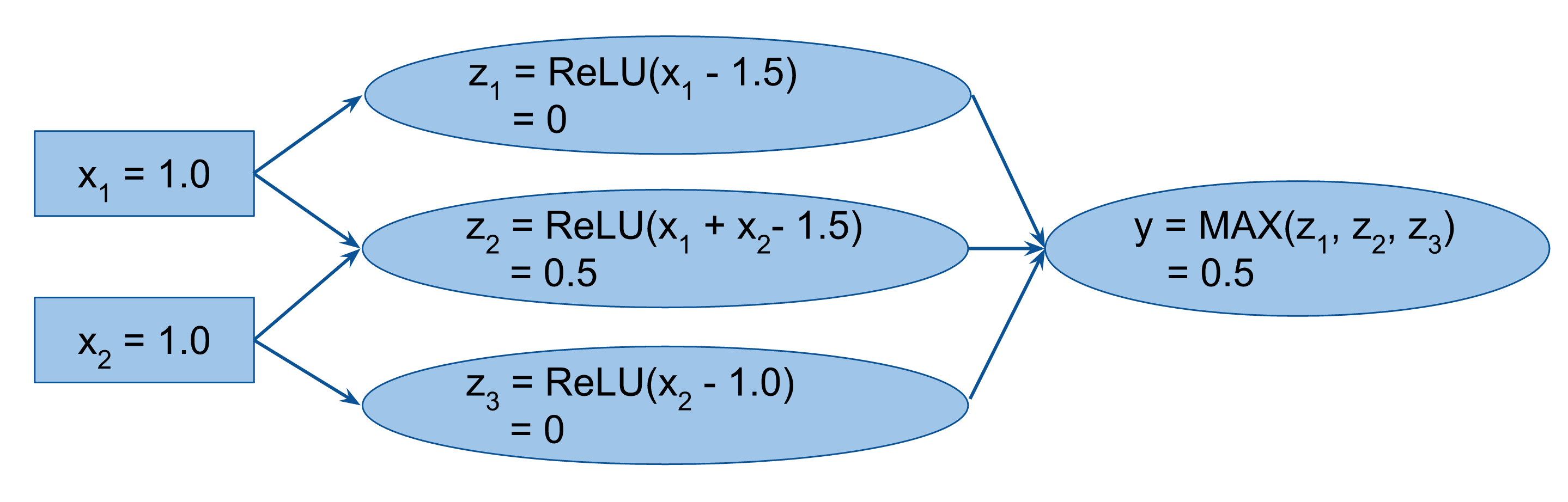
(b) $\begin{array}[]{ll}\mbox{Integrated gradients}&x_{1}=0.25,~{}x_{2}=0.25\\ \mbox{DeepLift}&x_{1}=0.25,~{}x_{2}=0.25\\ \mbox{Layer-wise relevance propagation}&x_{1}=0.25,~{}x_{2}=0.25\\ \mbox{DeConvNet}&x_{1}=1.0,~{}x_{2}=1.0\\ \mbox{Guided backpropagation}&x_{1}=1.0,~{}x_{2}=1.0\\ \end{array}$

Figure 14: Attributions for two functionally equivalent networks using integrated gradients, DeepLift (Shrikumar et al. (2016)), Layer-wise relevance propagation (Binder et al. (2016)), DeConvNets (Zeiler & Fergus (2014)), and Guided backpropagation (Springenberg et al. (2014)). The input is $x_{1}=1.0,~{}x_{2}=1.0$. The reference input for the DeepLift method is $x_{1}=0,~{}x_{2}=0$. All methods except integrated gradients provide different attributions for the two networks.

While there has been other work (see Section 2.8) to address this problem, these techniques involve instrumenting the network. This instrumentation currently involves significant developer effort because they are not primitive operations in standard machine learning libraries. Besides, these techniques are not simple to understand—they invert the operation of the network in different ways, and have their own peculiarities—for instance, the feature importances are not invariant over networks that compute the exact same function (see Figure 14).

In contrast, the method we propose builds on the very familiar, primitive concept of the gradient—all it involves is inspecting the gradients of a few carefully chosen counterfactual inputs that are scaled versions of the initial input. This allows anyone who knows how to extract gradients—presumably even novice practitioners that are not very familiar with the network’s implementation—to debug the network. Ultimately, this seems essential to ensuring that deep networks perform predictably when deployed.

2 Our Technique

2.1 Gradients Do Not Reflect Feature Importance

Let us start by investigating the performance of gradients as a measure of feature importance. We use an object recognition network built using the GoogleNet architecture (Szegedy et al. (2014)) as a running example; we refer to this network by its codename Inception. (We present applications of our techniques to other networks in Section 3.) The network has been trained on the ImageNet object recognition dataset (Russakovsky et al. (2015)). It is is $22$ layers deep with a softmax layer on top for classifying images into one of the $1000$ ImageNet object classes. The input to the network is a $224\times 224$ sized RGB image.

Before evaluating the use of gradients for feature importance, we introduce some basic notation that is used throughout the paper.

We represent a $224\times 224$ sized RGB image as a vector in $\mathsf{R}^{224\times 224\times 3}$. Let $\mathsf{Incp}^{L}:\mathsf{R}^{224\times 224\times 3}\rightarrow[0,1]$ be the function represented by the Inception network that computes the softmax score for the object class labeled $L$. Let $\bigtriangledown\mathsf{Incp}^{L}(\mathsf{img})$ be the gradients of $\mathsf{Incp}^{L}$ at the input image $\mathsf{img}$. Thus, the vector $\bigtriangledown\mathsf{Incp}^{L}(\mathsf{img})$ is the same size as the image and lies in $\mathsf{R}^{224\times 224\times 3}$. As a shorthand, we write $\bigtriangledown\mathsf{Incp}^{L}_{i,j,c}(\mathsf{img})$ for the gradient of a specific pixel $(i,j)$ and color channel $c\in\{R,G,B\}$.

We compute the gradients of $\mathsf{Incp}^{L}$ (with respect to the image) for the highest-scoring object class, and then aggregate the gradients $\bigtriangledown\mathsf{Incp}^{L}(\mathsf{img})$ along the color dimension to obtain pixel importance scores.

$$\forall i,j:\mathcal{P}^{L}_{i,j}(\mathsf{img})~{}::=~{}\Sigma_{c\in\{R,G,B\}}|\bigtriangledown\mathsf{Incp}^{L}_{i,j,c}(\mathsf{img})|$$ (1)

Next, we visualize pixel importance scores by scaling the intensities of the pixels in the original image in proportion to their respective scores; thus, higher the score brighter would be the pixel. Figure 1(a) shows a visualization for an image for which the highest scoring object class is “reflex camera” with a softmax score of $0.9938$.

(a) Original image.

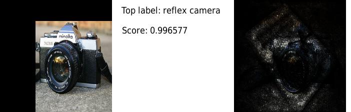
(b) Ablated image.

Figure 1: Pixel importance using gradients at the image.

Intuitively, one would expect the the high gradient pixels for this classification to be ones falling on the camera or those providing useful context for the classification (e.g., the lens cap). However, most of the highlighted pixels seem to be on the left or above the camera, which to a human seem not essential to the prediction. This could either mean that (1) the highlighted pixels are somehow important for the internal computation performed by the Inception network, or (2) gradients of the image fail to appropriately quantify pixel importance.

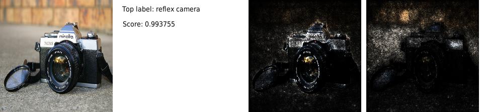
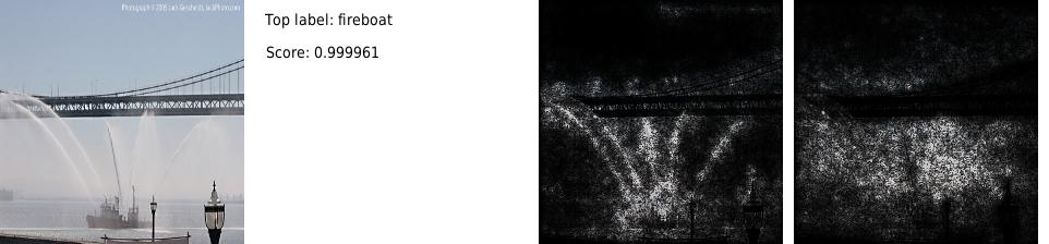
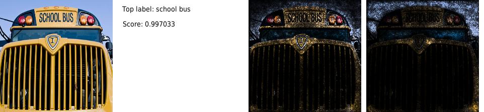
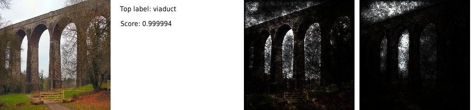
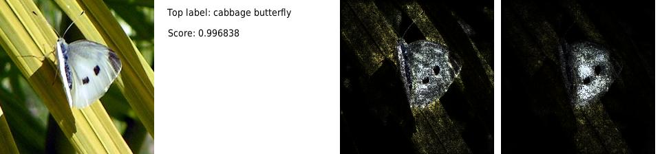
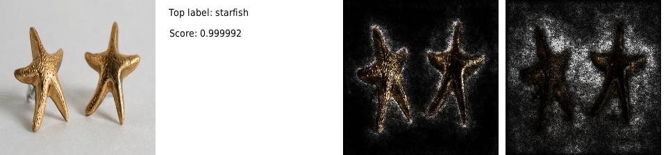
Figure 4: Comparing integrated gradients with gradients at the image. Left-to-right: original input image, label and softmax score for the highest scoring class, visualization of integrated gradients, visualization of gradients at the image. Notice that the visualizations obtained from integrated gradients are better at reflecting distinctive features of the image.

Let us consider hypothesis (1). In order to test it we ablate parts of the image on the left and above the camera (by zeroing out the pixel intensities) and run the ablated image through the Inception network. See Figure 1(b). The top predicted category still remains “reflex camera” with a softmax score of $0.9966$ — slightly higher than before. This indicates that the ablated portions are indeed irrelevant to the classification. On computing gradients of the ablated image, we still find that most of the high gradient pixels lie outside of the camera. This suggests that for this image, it is in fact hypothesis (2) that holds true. Upon studying more images (see Figure 4), we find that the gradients often fail to highlight the relevant pixels for the predicted object label.

2.2 Saturation

In theory, it is easy to see that the gradients may not reflect feature importance if the prediction function flattens in the vicinity of the input, or equivalently, the gradient of the prediction function with respect to the input is tiny in the vicinity of the input vector. This is what we call saturation, which has also been reported in previous work (Shrikumar et al. (2016), Glorot & Bengio (2010)).

We analyze how widespread saturation is in the Inception network by inspecting the behavior of the network on counterfactual images obtained by uniformly scaling pixel intensities from zero to their values in an actual image. Formally, given an input image $\mathsf{img}\in\mathsf{R}^{224\times 224\times 3}$, the set of counterfactual images is

$$\{\alpha~{}\mathsf{img}~{}|~{}0\leq\alpha\leq 1\}$$ (2)

Figure 2(a) shows the trend in the softmax output of the highest scoring class, for thirty randomly chosen images form the ImageNet dataset. More specifically, for each image $\mathsf{img}$, it shows the trend in $\mathsf{Incp}^{L}(\alpha~{}\mathsf{img})$ as $\alpha$ varies from zero to one with $L$ being the label of highest scoring object class for $\mathsf{img}$. It is easy to see that the trend flattens (saturates) for all images $\alpha$ increases. Notice that saturation is present even for images whose final score is significantly below $1.0$. Moreover, for a majority of images, saturation happens quite soon when $\alpha=0.2$.

One may argue that since the output of the Inception network is the result of applying the softmax function to a vector of activation values, the saturation is expected due to the squashing property of the softmax function. However, as shown in Figure 2(b), we find that even the pre-softmax activation scores for the highest scoring class saturate.

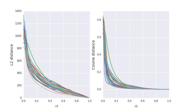
Layer mixed5b

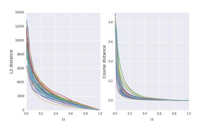
Layer mixed4d

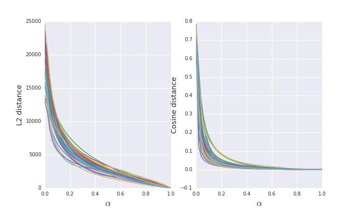
Layer mixed4b

Layer mixed3b

Figure 12: Saturation in intermediate layers of Inception. For each layer we plot the L2 and Cosine distance between the activation vector for a scaled down image and the actual input image, with respect to the scaling parameter. Each plot shows the trend for 30 randomly chosen images from the ImageNet dataset. Notice that trends in all plots flatten as the scaling parameter increases. For the deepest Inception layer mixed5b, the Cosine distance to the activation vector at the image is less than $0.01$ when $\alpha>0.6$, which is really tiny given that this layer has $50176$ neurons.

In fact, to our surprise, we found that the saturation is inherently present in the Inception network and the outputs of the intermediate layers also saturate. We plot the distance between the intermediate layer neuron activations for a scaled down input image and the actual input image with respect to the scaling parameter, and find that the trend flattens. Due to lack of space, we provide these plots in Figure 12 in the appendix.

It is quite clear from these plots that saturation is widespread across images in the Inception network, and there is a lot more activity in the network for counterfactual images at relatively low values of the scaling parameter $\alpha$. This observation forms the basis of our technique for quantifying feature importance.

Note that it is well known that the saturation of gradients prevent the model from converging to a good quality minima (Glorot & Bengio (2010)). So one may expect good quality models to not have saturation and hence for the (final) gradients to convey feature importance. Clearly, our observations on the Inception model show that this is not the case. It has good prediction accuracy, but also exhibits saturation (see Figure 2). Our hypothesis is that the gradients of important features are not saturated early in the training process. The gradients only saturate after the features have been learned adequately, i.e., the input is far away from the decision boundary.

2.3 Interior Gradients

We study the importance of input features in a prediction made for an input by examining the gradients of the counterfactuals obtained by scaling the input; we call this set of gradients interior gradients.

While the method of examining gradients of counterfactual inputs is broadly applicable to a wide range of networks, we first explain it in the context of Inception. Here, the counterfactual image inputs we consider are obtained by uniformly scaling pixel intensities from zero to their values in the actual image (this is the same set of counterfactuals that was used to study saturation). The interior gradients are the gradients of these images.

$$\mathsf{InteriorGrads}(\mathsf{img})~{}::=~{}\{\bigtriangledown\mathsf{Incp}(\alpha~{}\mathsf{img})~{}|~{}0\leq\alpha\leq 1\}$$ (3)

These interior gradients explore the behavior of the network along the entire scaling curve depicted in Figure 2(a), rather than at a specific point. We can aggregate the interior gradients along the color dimension to obtain interior pixel importance scores using equation 1.

$$\mathsf{InteriorPixelImportance}(\mathsf{img})~{}::=~{}\{\mathcal{P}(\alpha~{}\mathsf{img})~{}|~{}0\leq\alpha\leq 1\}$$ (4)

We individually visualize the pixel importance scores for each scaling parameter $\alpha$ by scaling the intensities of the pixels in the actual image in proportion to their scores. The visualizations show how the importance of each pixel evolves as we scale the image, with the last visualization being identical to one generated by gradients at the actual image. In this regard, the interior gradients offer strictly more insight into pixel importance than just the gradients at the actual image.

Figure 3 shows the visualizations for the “reflex camera” image from Figure  1(a) for various values of the scaling parameter $\alpha$. The plot in the top right corner shows the trend in the absolute magnitude of the average pixel importance score. The magnitude is significantly larger at lower values of $\alpha$ and nearly zero at higher values — the latter is a consequence of saturation. Note that each visualization is only indicative of the relative distribution of the importance scores across pixels and not the absolute magnitude of the scores, i.e., the later snapshots are responsible for tiny increases in the scores as the chart in the top right depicts.

The visualizations show that at lower values of $\alpha$, the pixels that lie on the camera are most important, and as $\alpha$ increases, the region above the camera gains importance. Given the high magnitude of gradients at lower values of $\alpha$, we consider those gradients to be the primary drivers of the final prediction score. They are more indicative of feature importance in the prediction compared to the gradients at the actual image (i.e., when $\alpha=1$).

The visualizations of the interior pixel gradients can also be viewed together as a single animation that chains the visualizations in sequence of the scaling parameter. This animation offers a concise yet complete summary of how pixel importance moves around the image as the scaling parameter increase from zero to one.

Rationale.  While measuring saturation via counterfactuals seems natural, using them for quantifying feature importance deserves some discussion. The first thing one may try to identify feature importance is to examine the deep network like one would with human authored code. This seems hard; just as deep networks employ distributed representations (such as embeddings), they perform convoluted (pun intended) distributed reasoning. So instead, we choose to probe the network with several counterfactual inputs (related to the input at hand), hoping to trigger all the internal workings of the network. This process would help summarize the effect of the network on the protagonist input; the assumption being that the input is human understandable. Naturally, it helps to work with gradients in this process as via back propagation, they induce an aggregate view over the function computed by the neurons.

Interior gradients use counterfactual inputs to artifactually induce a procedure on how the network’s attention moves across the image as it compute the final prediction score. From the animation, we gather that the network focuses on strong and distinctive patterns in the image at lower values of the scaling parameter, and subtle and weak patterns in the image at higher values. Thus, we speculate that the network’s computation can be loosely abstracted by a procedure that first recognize distinctive features of the image to make an initial prediction, and then fine tunes (these are small score jumps as the chart in Figure 3 shows) the prediction using weaker patterns in the image.

(a) Softmax score for top label

(b) Pre-softmax score for top label

Figure 2: Saturation in Inception

Input image and trend of the pixel importance scores obtained from interior gradients.

$\alpha=0.02$

$\alpha=0.04$

$\alpha=0.06$

$\alpha=0.08$

$\alpha=0.1$

$\alpha=0.2$

$\alpha=0.4$

$\alpha=0.6$

$\alpha=0.8$

$\alpha=1.0$

Figure 3: Visualization of interior gradients. Notice that the visualizations at lower values of the scaling parameter ($\alpha$) are sharper and much better at surfacing important features of the input image.

2.4 Cumulating Interior Gradients

A different summarization of the interior gradients can be obtained by cumulating them. While there are a few ways of cumulating counterfactual gradients, the approach we take has the nice attribution property (Proposition 1) that the feature importance scores approximately add up to the prediction score. The feature importance scores are thus also referred to as attributions.

Notice that the set of counterfactual images $\{\alpha~{}\mathsf{img}~{}|~{}0\leq\alpha\leq 1\}$ fall on a straight line path in $\mathsf{R}^{224\times 224\times 3}$. Interior gradients — which are the gradients of these counterfactual images — can be cumulated by integrating them along this line. We call the resulting gradients as integrated gradients. In what follows, we formalize integrated gradients for an arbitrary function $F:\mathsf{R}^{n}\rightarrow[0,1]$ (representing a deep network), and an arbitrary set of counterfactual inputs falling on a path in $\mathsf{R}^{n}$.

Let $x\in\mathsf{R}^{n}$ be the input at hand, and $\gamma=(\gamma_{1},\ldots,\gamma_{n}):[0,1]\rightarrow\mathsf{R}^{n}$ be a smooth function specifying the set of counterfactuals; here, $\gamma(0)$ is the baseline input (for Inception, a black image), and $\gamma(1)$ is the actual input (for Inception, the image being studied). Specifically, $\{\gamma(\alpha)~{}|~{}0\leq\alpha\leq 1\}$ is the set of counterfactuals (for Inception, a series of images that interpolate between the black image and the actual input).

The integrated gradient along the $i^{th}$ dimension for an input $x\in\mathsf{R}^{n}$ is defined as follows.

$$\mathsf{IntegratedGrads}_{i}(x)::=\int_{\alpha=0}^{1}\tfrac{\partial F(\gamma(\alpha))}{\partial\gamma_{i}(\alpha)}~{}\tfrac{\partial\gamma_{i}(\alpha)}{\partial\alpha}~{}d\alpha$$ (5)

where $\tfrac{\partial F(x)}{\partial x_{i}}$ is the gradient of $F$ along the $i^{th}$ dimension at $x$.

A nice technical property of the integrated gradients is that they add up to the difference between the output of $F$ at the final counterfactual $\gamma(1)$ and the baseline counterfactual $\gamma(0)$. This is formalized by the proposition below, which is an instantiation of the fundamental theorem of calculus for path integrals.

Proposition 1

If $F:\mathsf{R}^{n}\rightarrow\mathsf{R}$ is differentiable almost everywhere , and $\gamma:[0,1]\rightarrow\mathsf{R}^{n}$ is smooth then

$$\Sigma_{i=1}^{n}\mathsf{IntegratedGrads}_{i}(x)=F(\gamma(1))-F(\gamma(0))$$

For most deep networks, it is possible to choose counterfactuals such that the prediction at the baseline counterfactual is near zero ($F(\gamma(0))\approx 0$). For instance, for the Inception network, the counterfactual defined by the scaling path satisfies this property as $\mathsf{Incp}(0^{224\times 224\times 3})\approx 0$. In such cases, it follows from the Proposition that the integrated gradients form an attribution of the prediction output $F(x)$, i.e., they almost exactly distribute the output to the individual input features.

The additivity property provides a form of sanity checking for the integrated gradients and ensures that we do not under or over attribute to features. This is a common pitfall for attribution schemes based on feature ablations, wherein, an ablation may lead to small or a large change in the prediction score depending on whether the ablated feature interacts disjunctively or conjunctively to the rest of the features. This additivity is even more desirable when the network’s score is numerically critical, i.e., the score is not used purely in an ordinal sense. In this case, the attributions (together with additivity) guarantee that the attributions are in the units of the score, and account for all of the score.

We note that these path integrals of gradients have been used to perform attribution in the context of small non-linear polynomials (Sun & Sundararajan (2011)), and also within the cost-sharing literature in economics where function at hand is a cost function that models the cost of a project as a function of the demands of various participants, and the attributions correspond to cost-shares. The specific “path” we use corresponds to a cost-sharing method called Aumann-Shapley (Aumann & Shapley (1974)).

Computing integrated gradients.  The integrated gradients can be efficiently approximated by Riemann sum, wherein, we simply sum the gradients at points occurring at sufficiently small intervals along the path of counterfactuals.

$$\mathsf{IntegratedGrads}_{i}^{approx}(x)::=\Sigma_{k=1}^{m}\tfrac{\partial F(\gamma(k/m))}{\partial\gamma_{i}(\alpha)}~{}(\gamma(\tfrac{k}{m})-\gamma(\tfrac{k-1}{m}))$$ (6)

Here $m$ is the number of steps in the Riemman approximation of the integral. Notice that the approximation simply involves computing the gradient in a for loop; computing the gradient is central to deep learning and is a pretty efficient operation. The implementation should therefore be straightforward in most deep learning frameworks. For instance, in TensorFlow (ten ), it essentially amounts to calling tf.gradients in a loop over the set of counterfactual inputs (i.e., $\gamma(\tfrac{k}{m})~{}\mbox{for}~{}k=1,\ldots,m$), which could also be batched. Going forward, we abuse the term “integrated gradients” to refer to the approximation described above.

Integrated gradients for Inception.  We compute the integrated gradients for the Inception network using the counterfactuals obtained by scaling the input image; $\gamma(\alpha)=\alpha~{}\mathsf{img}$ where $\mathsf{img}$ is the input image. Similar to the interior gradients, the integrated gradients can also be aggregated along the color channel to obtain pixel importance scores which can then be visualized as discussed earlier. Figure 4 shows these visualizations for a bunch of images. For comparison, it also presents the corresponding visualization obtained from the gradients at the actual image. From the visualizations, it seems quite evident that the integrated gradients are better at capturing important features.

Attributions are independent of network implementation.  Two networks may be functionally equivalent despite having very different internal structures. See Figure 14 in the appendix for an example. Ideally, feature attribution should only be determined by the functionality of the network and not its implementation. Attributions generated by integrated gradients satisfy this property by definition since they are based only on the gradients of the function represented by the network.

In contrast, this simple property does not hold for all feature attribution methods known to us, including, DeepLift (Shrikumar et al. (2016)), Layer-wise relevance propagation (LRP) (Binder et al. (2016)), Deconvolution networks (DeConvNets) (Zeiler & Fergus (2014)), and Guided back-propagation (Springenberg et al. (2014)) (a counter-example is given in Figure 14). We discuss these methods in more detail in Section 2.8

2.5 Evaluating Our Approach

We discuss an evaluation of integrated gradients as a measure of feature importance, by comparing them against (final) gradients.

Pixel ablations.  The first evaluation is based on a method by Samek et al. (2015). Here we ablate the top $5000$ pixels ($10\%$ of the image) by importance score, and compute the score drop for the highest scoring object class. The ablation is performed $100$ pixels at a time, in a sequence of $50$ steps. At each perturbation step $k$ we measure the average drop in score up to step $k$. This quantity is referred to a area over the perturbation curve (AOPC) by Samek et al. (2015).

Figure 5 shows the AOPC curve with respect to the number of perturbation steps for integrated gradients and gradients at the image. AOPC values at each step represent the average over a dataset of $150$ randomly chosen images. It is clear that ablating the top pixels identified by integrated gradients leads to a larger score drop that those identified by gradients at the image.

Having said that, we note an important issue with the technique. The images resulting from pixel perturbation are often unnatural, and it could be that the scores drop simply because the network has never seen anything like it in training.

Localization.  The second evaluation is to consider images with human-drawn bounding boxes around objects, and compute the percentage of pixel attribution inside the bounding box. We use the 2012 ImageNet object localization challenge dataset to get a set of human-drawn bounding boxes. We run our evaluation on $100$ randomly chosen images satisfying the following properties — (1) the total size of the bounding box(es) is less than two thirds of the image size, and (2) ablating the bounding box significantly drops the prediction score for the object class. (1) is for ensuring that the boxes are not so large that the bulk of the attribution falls inside them by definition, and (2) is for ensuring that the boxed part of the image is indeed responsible for the prediction score for the image. We find that on $82$ images the integrated gradients technique leads to a higher fraction of the pixel attribution inside the box than gradients at the actual image. The average difference in the percentage pixel attribution inside the box for the two techniques is $8.4\%$.

While these results are promising, we note the following caveat. Integrated gradients are meant to capture pixel importance with respect to the prediction task. While for most objects, one would expect the pixel located on the object to be most important for the prediction, in some cases the context in which the object occurs may also contribute to the prediction. The “cabbage butterfly” image from Figure 4 is a good example of this where the pixels on the leaf are also surfaced by the integrated gradients.

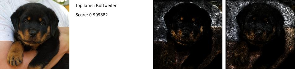
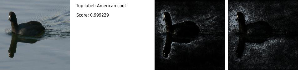
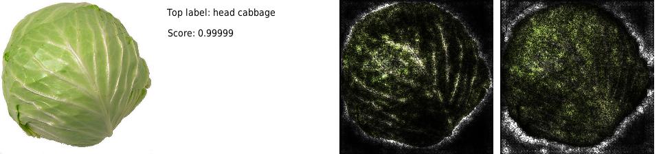
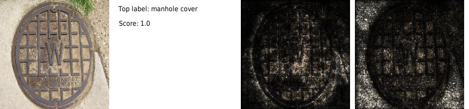
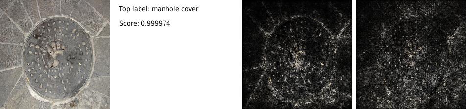
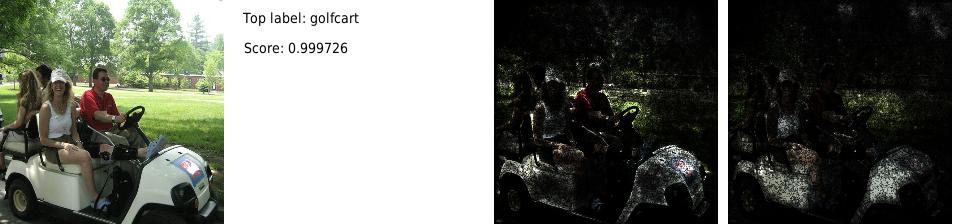
Figure 11: More visualizations comparing integrated gradients with gradients at the image. Left-to-right: original input image, label and softmax score for the highest scoring class, visualization of integrated gradients, visualization of gradients at the image.

Eyeballing.  Ultimately, it was hard to come up with a perfect evaluation technique. So we did spend a large amount of time applying and eyeballing the results of our technique to various networks—the ones presented in this paper, as well as some networks used within products. For the Inception network, we welcome you to eyeball more visualizations in Figure 11 in the appendix and also at: https://github.com/ankurtaly/Attributions. While we found our method to beat gradients at the image for the most part, this is clearly a subjective process prone to interpretation and cherry-picking, but is also ultimately the measure of the utility of the approach—debugging inherently involves the human.

Finally, also note that we did not compare against other whitebox attribution techniques (e.g., DeepLift (Shrikumar et al. (2016))), because our focus was on black-box techniques that are easy to implement, so comparing against gradients seems like a fair comparison.

2.6 Debugging networks

Despite the widespread application of deep neural networks to problems in science and technology, their internal workings largely remain a black box. As a result, humans have a limited ability to understand the predictions made by these networks. This is viewed as hindrance in scenarios where the bar for precision is high, e.g., medical diagnosis, obstacle detection for robots, etc. (dar (2016)). Quantifying feature importance for individual predictions is a first step towards understanding the behavior of the network; at the very least, it helps debug misclassified inputs, and sanity check the internal workings. We present evidence to support this below.

We use feature importance to debug misclassifications made by the Inception network. In particular, we consider images from the ImageNet dataset where the groundtruth label for the image not in the top five labels predicted by the Inception network. We use interior gradients to compute pixel importance scores for both the Inception label and the groundtruth label, and visualize them to gain insight into the cause for misclassification.

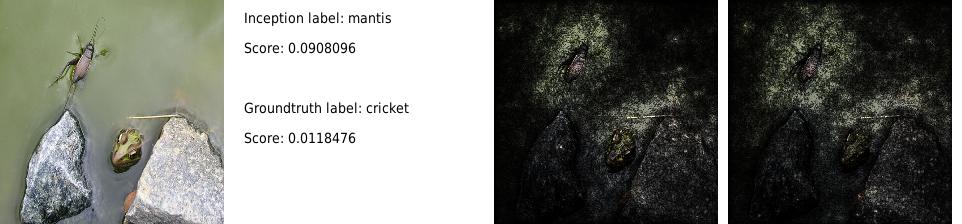
Figure 6: Interior gradients of misclassified images. Left-to-right: Original image, Softmax score for the top label assigned by the Inception network and the groundtruth label provided by ImageNet, visualization of integrated gradients w.r.t. Inception label, visualization of integrated gradients w.r.t. groundtruth label.

Figure 6 shows the visualizations for two misclassified images. The top image genuinely has two objects, one corresponding to the groundtruth label and other corresponding to the Inception label. We find that the interior gradients for each label are able to emphasize the corresponding objects. Therefore, we suspect that the misclassification is in the ranking logic for the labels rather than the recognition logic for each label. For the bottom image, we observe that the interior gradients are largely similar. Moreover, the cricket gets emphasized by the interior gradients for the “mantis” (Inception label). Thus, we suspect this to be a more serious misclassification, stemming from the recognition logic for the mantis.

2.7 Discussion

Faithfullness.  A natural question is to ask why gradients of counterfactuals obtained by scaling the input capture feature importance for the original image. First, from studying the visualizations in Figure 4, the results look reasonable in that the highlighted pixels capture features representative of the predicted class as a human would perceive them. Second, we confirmed that the network too seems to find these features representative by performing ablations. It is somewhat natural to expect that the Inception network is robust to to changes in input intensity; presumably there are some low brightness images in the training set.

However, these counterfactuals seem reasonable even for networks where such scaling does not correspond to a natural concept like intensity, and when the counterfactuals fall outside the training set; for instance in the case of the ligand-based virtual screening network (see Section 3.1). We speculate that the reason why these counterfactuals make sense is because the network is built by composing ReLUs. As one scales the input starting from a suitable baseline, various neurons activate, and the scaling process that does a somewhat thorough job of exploring all these events that contribute to the prediction for the input. There is an analogous argument for other operator such as max pool, average pool, and softmax—here the triggering events aren’t discrete but the argument is analogous.

Limitations of Approach.  We discuss some limitations of our technique; in a sense these are limitations of the problem statement and apply equally to other techniques that attribute to base input features.

• Inability to capture Feature interactions: The models could perform logic that effectively combines features via a conjunction or an implication-like operations; for instance, it could be that a molecule binds to a site if it has a certain structure that is essentially a conjunction of certain atoms and certain bonds between them. Attributions or importance scores have no way to represent these interactions.

• Feature correlations: Feature correlations are a bane to the understandability of all machine learning models. If there are two features that frequently co-occur, the model is free to assign weight to either or both features. The attributions would then respect this weight assignment. But, it could be that the specific weight assignment chosen by the model is not human-intelligible. Though there have been approaches to feature selection that reduce feature correlations (Yu & Liu (2003)), it is unclear how they apply to deep models on dense input.

2.8 Related work

Over the last few years, there has been a vast amount work on demystifying the inner workings of deep networks. Most of this work has been on networks trained on computer vision tasks, and deals with understanding what a specific neuron computes (Erhan et al. (2009); Le (2013)) and interpreting the representations captured by neurons during a prediction (Mahendran & Vedaldi (2015); Dosovitskiy & Brox (2015); Yosinski et al. (2015)).

Our work instead focuses on understanding the network’s behavior on a specific input in terms of the base level input features. Our technique quantifies the importance of each feature in the prediction. Known approaches for accomplishing this can be divided into three categories.

Gradient based methods.  The first approach is to use gradients of the input features to quantify feature importance (Baehrens et al. (2010); Simonyan et al. (2013)). This approach is the easiest to implement. However, as discussed earlier, naively using the gradients at the actual input does not accurate quantify feature importance as gradients suffer from saturation.

Score back-propagation based methods.  The second set of approaches involve back-propagating the final prediction score through each layer of the network down to the individual features. These include DeepLift (Shrikumar et al. (2016)), Layer-wise relevance propagation (LRP) (Binder et al. (2016)), Deconvolution networks (DeConvNets) (Zeiler & Fergus (2014)), and Guided back-propagation (Springenberg et al. (2014)). These methods largely differ in the backpropagation logic for various non-linear activation functions. While DeConvNets, Guided back-propagation and LRP rely on the local gradients at each non-linear activation function, DeepLift relies on the deviation in the neuron’s activation from a certain baseline input.

Similar to integrated gradients, the DeepLift and LRP also result in an exact distribution of the prediction score to the input features. However, as shown by Figure 14, the attributions are not invariant across functionally equivalent networks. Besides, the primary advantage of our method over all these methods is its ease of implementation. The aforesaid methods require knowledge of the network architecture and the internal neuron activations for the input, and involve implementing a somewhat complicated back-propagation logic. On the other hand, our method is agnostic to the network architectures and relies only on computing gradients which can done efficiently in most deep learning frameworks.

Model approximation based methods.  The third approach, proposed first by Ribeiro et al. (2016a; b), is to locally approximate the behavior of the network in the vicinity of the input being explained with a simpler, more interpretable model. An appealing aspect of this approach is that it is completely agnostic to the structure of the network and only deals with its input-output behavior. The approximation is learned by sampling the network’s output in the vicinity of the input at hand. In this sense, it is similar to our approach of using counterfactuals. Since the counterfactuals are chosen somewhat arbitrarily, and the approximation is based purely on the network’s output at the counterfactuals, the faithfullness question is far more crucial in this setting. The method is also expensive to implement as it requires training a new model locally around the input being explained.

Figure 5: AOPC (Samek et al. (2015)) for integrated gradients and gradients at image.

3 Applications to Other Networks

The technique of quantifying feature importance by inspecting gradients of counterfactual inputs is generally applicable across deep networks. While for networks performing vision tasks, the counterfactual inputs are obtained by scaling pixel intensities, for other networks they may be obtained by scaling an embedding representation of the input.

As a proof of concept, we apply the technique to the molecular graph convolutions network of Kearnes et al. (2016) for ligand-based virtual screening and an LSTM model (Zaremba et al. (2014)) for the language modeling of the Penn Treebank dataset (Marcus et al. (1993)).

3.1 Ligand-Based Virtual Screening

The Ligand-Based Virtual Screening problem is to predict whether an input molecule is active against a certain target (e.g., protein or enzyme). The process is meant to aid the discovery of new drug molecules. Deep networks built using molecular graph convolutions have recently been proposed by Kearnes et al. (2016) for solving this problem.

Once a molecule has been identified as active against a target, the next step for medicinal chemists is to identify the molecular features—formally, pharmacophores—that are responsible for the activity. This is akin to quantifying feature importance, and can be achieved using the method of integrated gradients. The attributions obtained from the method help with identifying the dominant molecular features, and also help sanity check the behavior of the network by shedding light on its inner workings. With regard to the latter, we discuss an anecdote later in this section on how attributions surfaced an anomaly in W1N2 network architecture proposed by Kearnes et al. (2016).

Defining the counterfactual inputs.  The first step in computing integrated gradients is to define the set of counterfactual inputs. The network requires an input molecule to be encoded by hand as a set of atom and atom-pair features describing the molecule as an undirected graph. Atoms are featurized using a one-hot encoding specifying the atom type (e.g., C, O, S, etc.), and atom-pairs are featurized by specifying either the type of bond (e.g., single, double, triple, etc.) between the atoms, or the graph distance between them

The counterfactual inputs are obtained by scaling down the molecule features down to zero vectors, i.e., the set $\{\alpha\mathsf{Features}(\mathsf{mol})~{}|~{}0\leq\alpha\leq 1\}$ where $\mathsf{Features}(mol)$ is an encoding of the molecule into atom and atom-pair features.

The careful reader might notice that these counterfactual inputs are not valid featurizations of molecules. However, we argue that they are still valid inputs for the network. First, all opera- tors in the network (e.g., ReLUs, Linear filters, etc.) treat their inputs as continuous real numbers rather than discrete zeros and ones. Second, all fields of the counterfactual inputs are bounded be- tween zero and one, therefore, we don’t expect them to appear spurious to the network. We discuss this further in section 2.7

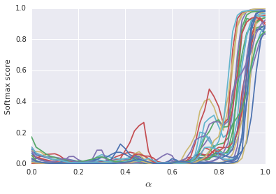
(a) Softmax score for task

(b) Sum of the feature gradients

Figure 13: Saturation in the W2N2 network (Kearnes et al. (2016)). Plots for the softmax score for task PCBA-58834, and the sum of the feature gradients w.r.t. the same task for twenty molecules. All molecules are active against the task

In what follows, we discuss the behavior of a network based on the W2N2-simple architecture proposed by Kearnes et al. (2016). On inspecting the behavior of the network over counterfactual inputs, we observe saturation here as well. Figure 13(a) shows the trend in the softmax score for the task PCBA-588342 for twenty five active molecules as we vary the scaling parameter $\alpha$ from zero to one. While the overall saturated region is small, saturation does exist near vicinity of the input ($0.9\leq\alpha\leq 1$). Figure 13(b) in the appendix shows that the total feature gradient varies significantly along the scaling path; thus, just the gradients at the molecule is fully indicative of the behavior of the network.

Visualizing integrated gradients.  We cumulate the gradients of these counterfactual inputs to obtain an attribution of the prediction score to each atom and atom-pair feature. Unlike image inputs, which have dense features, the set of input features for molecules are sparse. Consequently, the attributions are sparse and can be inspected directly. Figure 7 shows heatmaps for the atom and atom-pair attributions for a specific molecule.

Using the attributions, one can easily identify the atoms and atom-pairs that that have a strongly positive or strongly negative contribution. Since the attributions add up to the final prediction score (see Proposition 1), the attribution magnitudes can be use for accounting the contributions of each feature. For instance, the atom-pairs that have a bond between them contribute cumulatively contribute $46\%$ of the prediction score, while all other atom pairs cumulatively contribute $-3\%$.

We presented the attributions for $100$ molecules active against a specific task to a few chemists. The chemists were able to immediately spot dominant functional groups (e.g., aromatic rings) being surfaced by the attributions. A next step could be cluster the aggregate the attributions across a large set of molecules active against a specific task to identify a common denominator of features shared by all active molecules.

Figure 7: Attribution for a molecule under the W2N2 network (Kearnes et al. (2016)). The molecules is active on task PCBA-58432.

Identifying Dead Features.  We now discuss how attributions helped us spot an anomaly in the W1N2 architecture. On applying the integrated gradients method to the W1N2 network, we found that several atoms in the same molecule received the exact same attribution. For instance, for the molecule in Figure 7, we found that several carbon atoms at positions $2$, $3$, $14$, $15$, and $16$ received the same attribution of $0.0043$ despite being bonded to different atoms, for e.g., Carbon at position $3$ is bonded to an Oxygen whereas Carbon at position $2$ is not. This is surprising as one would expect two atoms with different neighborhoods to be treated differently by the network.

On investigating the problem further we found that since the W1N2 network had only one convolution layer, the atoms and atom-pair features were not fully convolved. This caused all atoms that have the same atom type, and same number of bonds of each type to contribute identically to the network. This is not the case for networks that have two or more convolutional layers.

Despite the aforementioned problem, the W1N2 network had good predictive accuracy. One hypothesis for this is that the atom type and their neighborhoods are tightly correlated; for instance an outgoing double bond from a Carbon is always to another Carbon or Oxygen atom. As a result, given the atom type, an explicit encoding of the neighborhood is not needed by the network. This also suggests that equivalent predictive accuracy can be achieved using a simpler “bag of atoms” type model.

3.2 Language Modeling

To apply our technique for language modeling, we study word-level language modeling of the Penn Treebank dataset (Marcus et al. (1993)), and apply an LSTM-based sequence model based on Zaremba et al. (2014). For such a network, given a sequence of input words, and the softmax prediction for the next word, we want to identify the importance of the preceding words for the score.

As in the case of the Inception model, we observe saturation in this LSTM network. To describe the setup, we choose 20 randomly chosen sections of the test data, and for each of them inspect the prediction score of the next word using the first 10 words. Then we give each of the 10 input words a weight of $\alpha\in[0,1]$, which is applied to scale their embedding vectors. In Figure 8, we plot the prediction score as a function of $\alpha$. For all except one curves, the curve starts near zero at $\alpha=0$, moves around in the middle, stabilizes, and turns flat around $\alpha=1$. For the interesting special case where softmax score is non-zero at $\alpha=0$, it turns out that that the word being predicted represents out of vocabulary words.

Figure 8: Softmax scores of the next word in the LSTM language model (Section 3.2)

[!h]

Sentence	the	shareholders	claimed	more	than	$ N millions in losses
Integrated gradients	-0.1814	-0.1363	0.1890	0.6609
Gradients	0.0007	-0.0021	0.0054	-0.0009

Figure 9: Prediction for than: 0.5307, total integrated gradient: 0.5322

Sentence	and	N	minutes	after	the	ual	trading
Integrated gradients (*1e-3)	0.0707	0.1286	0.3619	1.9796	-0.0063	4.1565	0.2213
Gradients (*1e-3)	0.0066	0.0009	0.0075	0.0678	0.0033	0.0474	0.0184
Sentence (Cont.)	halt	came	news	that	the	ual	group
Integrated gradients (*1e-3)	-0.8501	-0.4271	0.4401	-0.0919	0.3042
Gradients (*1e-3)	-0.0590	-0.0059	0.0511	0.0041	0.0349

Figure 10: Prediction for ual: 0.0062, total integrated gradient: 0.0063

In Table 9 and Table 10 we show two comparisons of gradients to integrated gradients. Due to saturation, the magnitudes of gradients are so small compared to the prediction scores that it is difficult to make sense of them. In comparison, (approximate) integrated gradients have a total amount close to the prediction, and seem to make sense. For example, in the first example, the integrated gradients attribute the prediction score of “than“ to the preceding word “more”. This makes sense as “than” often follows right after “more“ in English. On the other hand, standard gradient gives a slightly negative attribution that betrays our intuition. In the second example, in predicting the second “ual”, integrated gradients are clearly the highest for the first occurrence of “ual”, which is the only word that is highly predictive of the second “ual”. On the other hand, standard gradients are not only tiny, but also similar in magnitude for multiple words.

4 Conclusion

We present Interior Gradients, a method for quantifying feature importance. The method can be applied to a variety of deep networks without instrumenting the network, in fact, the amount of code required is fairly tiny. We demonstrate that it is possible to have some understanding of the performance of the network without a detailed understanding of its implementation, opening up the possibility of easy and wide application, and lowering the bar on the effort needed to debug deep networks.

We also wonder if Interior Gradients are useful within training as a measure against saturation, or indeed in other places that gradients are used.

Acknowledgments

We would like to thank Patrick Riley and Christian Szegedy for their helpful feedback on the technique and on drafts of this paper.

Appendix A Appendix

(a) $\begin{array}[]{ll}\mbox{Integrated gradients}&x_{1}=0.25,~{}x_{2}=0.25\\ \mbox{DeepLift}&x_{1}=\tfrac{0.5}{3},~{}x_{2}=\tfrac{1}{3}\\ \mbox{Layer-wise relevance propagation}&x_{1}=\tfrac{0.5}{3},~{}x_{2}=\tfrac{1}{3}\\ \mbox{DeConvNet}&x_{1}=1.25,~{}x_{2}=0.75\\ \mbox{Guided backpropagation}&x_{1}=1.25,~{}x_{2}=0.75\\ \end{array}$

References

- (1) TensorFlow. https://www.tensorflow.org/.
- dar (2016) Explainable Artificial Intelligence. http://www.darpa.mil/attachments/DARPA-BAA-16-53.pdf, 2016.
- Aumann & Shapley (1974) R. J. Aumann and L. S. Shapley. Values of Non-Atomic Games. Princeton University Press, Princeton, NJ, 1974.
- Baehrens et al. (2010) David Baehrens, Timon Schroeter, Stefan Harmeling, Motoaki Kawanabe, Katja Hansen, and Klaus-Robert Müller. How to explain individual classification decisions. Journal of Machine Learning Research, pp. 1803–1831, 2010.
- Binder et al. (2016) Alexander Binder, Grégoire Montavon, Sebastian Bach, Klaus-Robert Müller, and Wojciech Samek. Layer-wise relevance propagation for neural networks with local renormalization layers. CoRR, 2016. URL http://arxiv.org/abs/1604.00825.
- Dosovitskiy & Brox (2015) Alexey Dosovitskiy and Thomas Brox. Inverting visual representations with convolutional networks, 2015. URL http://arxiv.org/abs/1506.02753.
- Erhan et al. (2009) Dumitru Erhan, Yoshua Bengio, Aaron Courville, and Pascal Vincent. Visualizing higher-layer features of a deep network. Technical Report 1341, University of Montreal, 2009.
- Glorot & Bengio (2010) Xavier Glorot and Yoshua Bengio. Understanding the difficulty of training deep feedforward neural networks. In Artificial Intelligence and Statistics (AISTATS’10), 2010.
- Kearnes et al. (2016) Steven Kearnes, Kevin McCloskey, Marc Berndl, Vijay Pande, and Patrick Riley. Molecular graph convolutions: moving beyond fingerprints. Journal of Computer-Aided Molecular Design, pp. 595–608, 2016.
- Le (2013) Quoc V. Le. Building high-level features using large scale unsupervised learning. In International Conference on Acoustics, Speech, and Signal Processing (ICASSP), pp. 8595–8598, 2013.
- Mahendran & Vedaldi (2015) Aravindh Mahendran and Andrea Vedaldi. Understanding deep image representations by inverting them. In Conference on Computer Vision and Pattern Recognition (CVPR), pp. 5188–5196, 2015.
- Marcus et al. (1993) Mitchell P. Marcus, Beatrice Santorini, and Mary Ann Marcinkiewicz. Building a large annotated corpus of english: The penn treebank. Computational Linguistics, pp. 313–330, 1993.
- Ribeiro et al. (2016a) Marco Túlio Ribeiro, Sameer Singh 0001, and Carlos Guestrin. ”why should I trust you?”: Explaining the predictions of any classifier. In 22nd ACM International Conference on Knowledge Discovery and Data Mining, pp. 1135–1144. ACM, 2016a.
- Ribeiro et al. (2016b) Marco Túlio Ribeiro, Sameer Singh 0001, and Carlos Guestrin. Model-agnostic interpretability of machine learning. CoRR, 2016b. URL http://arxiv.org/abs/1606.05386.
- Russakovsky et al. (2015) Olga Russakovsky, Jia Deng, Hao Su, Jonathan Krause, Sanjeev Satheesh, Sean Ma, Zhiheng Huang, Andrej Karpathy, Aditya Khosla, Michael Bernstein, Alexander C. Berg, and Li Fei-Fei. ImageNet Large Scale Visual Recognition Challenge. International Journal of Computer Vision (IJCV), pp. 211–252, 2015.
- Samek et al. (2015) Wojciech Samek, Alexander Binder, Grégoire Montavon, Sebastian Bach, and Klaus-Robert Müller. Evaluating the visualization of what a deep neural network has learned. CoRR, 2015. URL http://arxiv.org/abs/1509.06321.
- Shrikumar et al. (2016) Avanti Shrikumar, Peyton Greenside, Anna Shcherbina, and Anshul Kundaje. Not just a black box: Learning important features through propagating activation differences. CoRR, 2016. URL http://arxiv.org/abs/1605.01713.
- Simonyan et al. (2013) Karen Simonyan, Andrea Vedaldi, and Andrew Zisserman. Deep inside convolutional networks: Visualising image classification models and saliency maps. CoRR, 2013. URL http://arxiv.org/abs/1312.6034.
- Springenberg et al. (2014) Jost Tobias Springenberg, Alexey Dosovitskiy, Thomas Brox, and Martin A. Riedmiller. Striving for simplicity: The all convolutional net. CoRR, 2014. URL http://arxiv.org/abs/1412.6806.
- Sun & Sundararajan (2011) Yi Sun and Mukund Sundararajan. Axiomatic attribution for multilinear functions. In 12th ACM Conference on Electronic Commerce (EC), pp. 177–178, 2011.
- Szegedy et al. (2014) Christian Szegedy, Wei Liu, Yangqing Jia, Pierre Sermanet, Scott E. Reed, Dragomir Anguelov, Dumitru Erhan, Vincent Vanhoucke, and Andrew Rabinovich. Going deeper with convolutions. CoRR, abs/1409.4842, 2014. URL http://arxiv.org/abs/1409.4842.
- Yosinski et al. (2015) Jason Yosinski, Jeff Clune, Anh Mai Nguyen, Thomas Fuchs, and Hod Lipson. Understanding neural networks through deep visualization. CoRR, 2015. URL http://arxiv.org/abs/1506.06579.
- Yu & Liu (2003) Lei Yu and Huan Liu. Feature selection for high-dimensional data: A fast correlation-based filter solution. In 20th International Conference on Machine Learning (ICML), pp. 856–863, 2003. URL http://www.aaai.org/Papers/ICML/2003/ICML03-111.pdf.
- Zaremba et al. (2014) Wojciech Zaremba, Ilya Sutskever, and Oriol Vinyals. Recurrent neural network regularization. CoRR, 2014. URL http://arxiv.org/abs/1409.2329.
- Zeiler & Fergus (2014) Matthew D. Zeiler and Rob Fergus. Visualizing and understanding convolutional networks. In 13th European Conference on Computer Vision (ECCV), pp. 818–833, 2014.