A lattice Boltzmann scheme with arbitrary Prandtl number and
specific heat ratio based on the polyatomic ES-BGK model

Abstract

A Boltzmann lattice scheme based on the polyatomic ellipsoidal statistical model (ES-BGK) is proposed, incorporating an arbitrary Prandtl number and a specific heat ratio. The Prandtl number is modulated by a parameter in the Gaussian distribution, while the specific heat ratio is adjusted by additional free degrees. The Gaussian distribution is expanded using Hermite polynomials, and a general formula for the Hermite coefficients of the Gaussian distribution is derived. Benchmark tests are conducted to validate the proposed scheme, with numerical results demonstrating good agreement with analytical solutions.

PACS numbers

47.11.-j, 47.10.-g, 47.40.-x

I Introduction

Over the past three decades, the Lattice Boltzmann Method (LBM) has been widely applied to a variety of complex flows, such as multiphase and multicomponent fluids Guo and Zhao (2005)Li et al. (2016), fluid flows through porous media Ferreol and Rothman (1995), turbulenceChen et al. (2003), magneto-hydrodynamicsRahmati and Najjarnezami (2016), and thermal fluidsYoshino et al. (2004). However, when LBM is applied to thermal fluids, it encounters some issues. Specifically, the Navier-Stokes equations (including the energy conversation equation) can be derived from the evolution equation via the Chapman-Enskog expansion, but the specific heat ratio and the Prandtl number are fixed. As a result, the transport coefficients obtained this way are not realistic for polyatomic molecule fluids.

To address this issue, some LB schemes combined with arbitrary specific heat ratio or Prandtl number have been proposed. To modify the specific heat ratio, new variables such as rotational velocity or rotational energy are introduced and discretized in the velocity space Kataoka and Tsutahara (2004); Watari (2007); Tsutahara et al. (2008); Nie et al. (2008). While these LB schemes have clear physical meanings and are easy to implement, they require the setting of parameters through experience. To modify the Prandtl number, a quasi-equilibrium or other similar element that controls the Prandtl number is introduced Frapolli et al. (2014); Chen et al. (1997); Yan-Biao et al. (2011); Soe et al. (1998). Some works give arbitrary specific heat ratio and Prandtl number at the same time (Dellar, 2008; Saadat et al., 2019).

Most of these schemes are based on the BGK collision model, which assumes that the molecule is monatomic. An alternative collision model, the Ellipsoidal Statistics Model (ES-BGK) Holway Jr (1965), has been proposed. The model has additional parameters, yielding satisfactory transport coefficients at the Navier-Stokes level and satisfying the entropy inequality ($H$-theorem) Andries et al. (2000); Andries and Perthame (2001); Andries et al. (2002); Brull and Schneider (2009); Meng et al. (2013a), which is an essential requirement for a successful LB scheme.

In this work, we present a novel LB scheme with an arbitrary Prandtl number (and an arbitrary specific heat ratio) based on the ES-BGK model. Our main contribution was deriving a general term formula for the Hermite coefficients of the Gaussian distribution, which facilitates the derivation of high-order terms of the Hermite coefficients. This general term formula makes the design of high-order LB schemes based on the ES-BGK model more straightforward and efficient. Consequently, the general term formula can be used to efficiently design LB schemes applied to 2D or 3D flows. Compared to existing schemes, the proposed LB scheme has several advantages. Its physical meaning is clear and it adheres to the $H$-theorem, which is essential for a lattice Boltzmann scheme. Additionally, it does not require parameters to be set through experience, and its implementation is much simpler, as it only requires rewriting the code of the equilibrium distribution function, while the other parts of the code and the basic structure remain unchanged.

II Polyatomic ES-BGK model

This section discusses the polyatomic ES-BGK model, which is characterized by the kinetic equation of the polyatomic distribution function $f(\bm{\xi},\bm{x},t,I)$Andries et al. (2000); Brull and Schneider (2009).

$$\frac{\partial f}{\partial t}+\bm{\xi}\cdot\frac{\partial f}{\partial\bm{x}}=\Omega,$$ (1)

where $f(\bm{\xi},\bm{x},t,I)$ is the distribution function with the particle velocity $\bm{\xi}$ and the internal energy $\epsilon(I)=I^{\frac{2}{N_{f}}}$ at position $\bm{x}$ and time $t$, $N_{f}$ being the additional degrees of freedom of the gas. The collision operator $\Omega(f)$ is given by

$$\Omega(f)=-\frac{1}{\tau(1-\nu+\nu\kappa)}(f-G[f]),$$ (2)

where $\tau$ is the relaxation time and $G[f]$ is the polyatomic Gaussian model. The parameters $-\frac{2}{3}\leqslant\nu<1$ and $0\leqslant\kappa\leqslant 1$ are introduced to modify the Prandtl number and the specific heat ratio.

The density $\rho$, macroscopic velocity $\bm{u}$, and total energy $E$, as well as the specific internal energy $e$, are defined by the moments of the distribution function $f$ as follows:

$$\rho= \int_{\mathbb{R}^{D}}\!\!\int_{\mathbb{R}^{+}}f\,d\bm{\xi}\,dI,$$ (3a)

$$\rho\bm{u}= \int_{\mathbb{R}^{D}}\!\!\int_{\mathbb{R}^{+}}\bm{\xi}f\,d\bm{\xi}\,dI,$$ (3b)

$$E=\frac{1}{2}\rho u^{2}+\rho e= \int_{\mathbb{R}^{D}}\!\!\int_{\mathbb{R}^{+}}(\frac{1}{2}\xi^{2}+I^{\frac{2}{N_{f}}})f\,d\bm{\xi}\,dI,$$ (3c)

where $D$ is the space dimension.

The specific internal energy $e$ can be expressed as the sum of two components: the internal energy of translational velocity $e_{tr}$ and the energy associated with the internal structure $e_{int}$, as follows:

$$e=e_{tr}+e_{int},$$ (4)

where

$$e_{tr} =\frac{1}{\rho}\int_{R^{D}}\!\!\int_{R^{+}}\frac{1}{2}(\bm{\xi}-\bm{u})^{2}fd\bm{\xi}d{I},$$ (5)

$$e_{int} =\frac{1}{\rho}\int_{R^{D}}\!\!\int_{R^{+}}I^{2/N_{f}}fd\bm{\xi}d{I}.$$ (6)

The relationship between temperature ($T$, $T_{tr}$, $T_{int}$) and the corresponding energy ($e$, $e_{tr}$, $e_{int}$) can be expressed as follows:

$$e=\frac{D+N_{f}}{2}R_{g}T_{eq},\quad e_{tr}=\frac{D}{2}R_{g}T_{tr},\quad e_{int}=\frac{N_{f}}{2}R_{g}T_{int},$$ (7)

where $R_{g}$ is the universal gas constant.

The state equation can be expressed as $p=\rho R_{g}T_{eq}$, where $p$ denotes the pressure.

The Generalized Gaussian Model is defined by the equation:

$$G[f]= \frac{\Lambda_{N_{f}}\rho}{\sqrt{det(2\pi\mathbb{\Lambda)}}}\frac{1}{R_{g}T_{rel}^{N_{f}/2}}$$

$$\times\exp{\Big{[}-\frac{1}{2}(\bm{\xi}-\bm{u})\cdot\bm{\Lambda}^{-1}\cdot(\bm{\xi}-\bm{u})-\frac{I^{\frac{2}{N_{f}}}}{R_{g}T_{rel}}\Big{]}},$$ (8)

where $\bm{\Lambda}$ is the corrected tensor given by

$$\bm{\Lambda}=(1-\kappa)[(1-\nu)R_{g}T_{tr}\bm{\delta}+\nu\bm{\sigma}]+\kappa R_{g}T_{eq}\bm{\delta},$$ (9)

$\bm{\sigma}$ is the opposite stress tensor,

$$\bm{\sigma}=\frac{1}{\rho}\int(\bm{\xi}-\bm{u})(\bm{\xi}-\bm{u})fd\bm{\xi},$$ (10)

and $\bm{\delta}$ is the unit tensor. The relaxation temperature $T_{rel}$ is defined as

$$T_{rel}=\kappa T_{eq}+(1-\kappa)T_{int},$$ (11)

and the constant $\Lambda_{N_{f}}$ is given by

$$\Lambda_{N_{f}}^{-1}\!=\!\int e^{-I^{2}/N_{f}}dI.$$ (12)

III Polyatomic ES-BGK model: Description with two distribution functions

The evolution equation of the polyatomic distribution function $f(\bm{\xi},\bm{x},t,I)$ can be expressed as

$$\frac{\partial}{\partial t}f+\bm{\xi}\cdot\frac{\partial}{\partial\bm{x}}f=-\frac{1}{\tau(1-\nu+\kappa\nu)}\left(f-G[f]\right),$$ (13)

where $\tau$, $\nu$, and $\kappa$ are constants. The kinetic equation can be reduced to two distribution functions, namely the mass distribution function $g(\bm{\xi})$ and the energy distribution function $h(\bm{\xi})$, as proposed by C.K.Chu Chu (1965a, b) and V.A.Rykov Rykov (1975). This approach has the advantage of reducing computational resources, as well as eliminating the need to discretize $\epsilon$ in the discrete velocity space when applied to the Lattice Boltzmann Method (LBM). The lattices employed in this scheme are DnQb models, which are simpler to design than those requiring the discretization of both the translational velocity of the particle and the newly introduced parameter Watari (2007); Tsutahara et al. (2008); Yudistiawan et al. (2010); Yan-Biao et al. (2011).

The distributions of $g(\bm{\xi},\bm{x},t)$ and $h(\bm{\xi},\bm{x},t)$ are defined by

$$g(\bm{\xi},\bm{x},t)= \int_{R^{+}}f(\bm{\xi},\bm{x},t,I)\mathrm{d}I,$$ (14a)

$$h(\bm{\xi},\bm{x},t)= \int_{R^{+}}I^{\frac{2}{N_{f}}}f(\bm{\xi},\bm{x},t,I)\mathrm{d}I.$$ (14b)

The macroscopic quantities are determined by the moments of the mass distribution $g(\bm{\xi})$ and the energy distribution $h(\bm{\xi})$ as follows:

$$\rho= \int_{R^{D}}g(\bm{\xi})\mathrm{d}\bm{\xi},$$ (15a)

$$\rho\bm{u}= \int_{R^{D}}\bm{\xi}g(\bm{\xi})\mathrm{d}\bm{\xi},$$ (15b)

$$\rho E= \int_{R^{D}}[\frac{1}{2}\xi^{2}g(\bm{\xi})+h(\bm{\xi})]\mathrm{d}\bm{\xi}.$$ (15c)

Integrating Eq.(  13) on $I$, we obtain the evolution equation of $g(\bm{\xi})$

$$\frac{\partial}{\partial t}g+\bm{\xi}\cdot\nabla g=-\frac{1}{\tau(1-\nu+\kappa\nu)}(g-G[g,h]),$$ (16)

where $G[g,h]$ is

$$G[g,h]=\frac{\rho}{\sqrt{\mathrm{det}(2\pi\mathbb{\Lambda})}}\exp\left[-\frac{1}{2}(\bm{\xi}-\bm{u})\cdot\bm{\Lambda}^{-1}\cdot(\bm{\xi}-\bm{u})\right].$$ (17)

Integrating Eq. ( 13) multiplied by $I^{\frac{2}{N_{f}}}$ over $I$, we obtain the evolution equation of $h(\bm{\xi})$ as

$$\frac{\partial}{\partial t}h+\bm{\xi}\cdot\nabla h=-\frac{1}{\tau(1-\nu+\kappa\nu)}(h-\frac{N_{f}}{2}R_{g}T_{\mathrm{rel}}G[g,h]).$$ (18)

From Eq.( 16) and ( 18), the Navier-Stokes equations with an arbitrary specific heat ratio and Prandtl number can be derived via the Chapman-Enskog expansion Andries et al. (2000); Ansumali et al. (2003). In the derived Navier-Stokes equations, the viscosity tensor is given by $\bm{\sigma}=\mu(\nabla\bm{u}+\bm{u}\nabla-\alpha\nabla\cdot\bm{u}\bm{\delta})$, where $\mu=\tau p/(1-\nu+\kappa\nu)$ is the viscosity coefficient and $\mu\alpha$ is the second viscosity coefficient, with $\alpha=(\gamma-1)-\frac{1-\kappa}{\kappa}(1-\nu)(\frac{D+2}{D}-\gamma)$. The specific heat ratio $\gamma$ and Prandtl number $Pr$ in the recovered Navier-Stokes equations are defined, respectively, as:

$$\gamma=\frac{N_{f}+D+2}{N_{f}+D},$$ (19)

$$Pr=\frac{1}{1-\nu+\kappa\nu},$$ (20)

where $2/3\leq Pr<+\infty$.

IV The General Term Formula for the Hermite Coefficients of the Gaussian distribution

The expansion of the Maxwell-Boltzmann distribution on the Hermite polynomials has been explored in the literature Grad (1949); Shim and Gatignol (2013); Mattila et al. (2014a). Here, we extend this discussion, expand the Gaussian distribution on the Hermite polynomials.

The identities given by Grad in Grad (1949), i.e. Eq. (4), (12) and (16), are employed in the following paragraphs. These are:

$$(\bm{x}+\bm{y})^{n} =\sum^{n}_{r=0}\bm{x}^{r}\bm{y}^{n-r},$$ (21)

$$\mu_{2n} =\int\omega(\bm{x})\bm{x}^{2n}d\bm{x}=\bm{\delta}^{n},$$ (22)

$$\bm{H}^{(n)}(\bm{x}) =\bm{x}^{n}-\bm{\delta}\bm{x}^{n-2}+\bm{\delta}^{2}\bm{x}^{n-4}+\cdots,$$ (23)

where $\bm{H}^{(n)}(\bm{x})$ is the Hermite polynomials and $\omega(\bm{x})$ is the weight function

$$\omega(\bm{x})=\displaystyle\frac{1}{\sqrt{(2\pi)^{D/2}}}\exp{(-\frac{x^{2}}{2})}.$$

The following equations are derived from the above identities:

$$\bm{H}^{(0)}(\bm{\xi}) =1,$$

$$\bm{H}^{(1)}(\bm{\xi}) =\bm{\xi},$$

$$\bm{H}^{(2)}(\bm{\xi}) =\bm{\xi}^{2}-\bm{\delta},$$

$$\bm{H}^{(3)}(\bm{\xi}) =\bm{\xi}^{3}-\bm{\delta}\bm{\xi},$$

$$\bm{H}^{(4)}(\bm{\xi}) =\bm{\xi}^{4}-\bm{\delta}\bm{\xi}^{2}+\bm{\delta}^{2},$$

$$\bm{H}^{(5)}(\bm{\xi}) =\bm{\xi}^{5}-\bm{\delta}\bm{\xi}^{3}+\bm{\delta}^{2}\bm{\xi},$$

$$\bm{H}^{(6)}(\bm{\xi}) =\bm{\xi}^{6}-\bm{\delta}\bm{\xi}^{4}+\bm{\delta}^{2}\bm{\xi}^{2}-\bm{\delta}^{3}$$

The identities given by Grad in Grad (1949), i.e. Eq. (4), (12) and (16), are employed in the following equations. These equations are derived from the identities, which involve the Hermite polynomials $\bm{H}^{(n)}(\bm{x})$ and the weight function $\omega(\bm{x})$.

The Gaussian distribution $G$ can be expressed as an expansion on the Hermite polynomial, as shown in Equation Eq.( 24):

$$G=\rho\omega(\bm{\xi})\sum_{n=0}^{\infty}\frac{1}{n!}\bm{a}^{(n)}\cdot\bm{H}^{(n)}(\bm{\xi}),$$ (24)

where $\bm{a}^{(n)}$ are the expansion coefficients and $\bm{H}^{(n)}(\bm{\xi})$ are the Hermite polynomials. The expansion coefficients $\bm{a}^{(n)}$ can be obtained by

$$\bm{a}^{(n)}=\frac{1}{\rho}\int\bm{H}^{(n)}(\bm{\xi})Gd\bm{\xi}.$$ (25)

By defining $(\bm{\xi}-\bm{u})\cdot\bm{\Lambda}^{-\frac{1}{2}}=\bm{\eta}$, we obtain $\bm{\xi}=\bm{u}+\bm{\eta}\cdot\bm{\Lambda}^{\frac{1}{2}}$. Inserting this and Eq.( 17) into Eq.( 25), we obtain

$$\bm{a}^{(n)}=\sum_{\alpha=0}^{[n/2]}\sum_{\beta=0}^{[n/2]-\alpha}(-1)^{\alpha}\bm{\delta}^{\alpha}\bm{\Lambda}^{\beta}\bm{u}^{n-2(\alpha+\beta)}.$$ (26)

The derivation of Eq. (26) can be found in Appendix. (A).

Defining $\chi\!=\!\alpha+\beta$, inserting $\chi$ into Eq( 26) and changing the ranges of the superscripts we obtain

$$\bm{a}^{(n)}= \sum_{\chi=0}^{[n/2]}\sum_{\beta=0}^{\chi}(-1)^{\beta}\bm{\Lambda}^{\beta}\bm{\delta}^{\chi-\beta}\bm{u}^{n-2\chi}$$

$$= \sum_{\chi=0}^{[n/2]}(\bm{\Lambda}-\bm{\delta)}^{\chi}\bm{u}^{n-2\chi}$$

$$= \sum_{\alpha=0}^{[n/2]}(\bm{\Lambda}-\bm{\delta)}^{\alpha}\bm{u}^{n-2\alpha}.$$

Finally, we obtain the general term formula for the Hermite coefficients of the Gaussian distribution $G$

$$\bm{a}^{(n)}=\sum_{\alpha=0}^{[n/2]}\sum_{\beta=0}^{\alpha}(-1)^{\alpha-\beta}\bm{\Lambda}^{\beta}\bm{\delta}^{\alpha-\beta}\bm{u}^{n-2\alpha}.$$ (27)

The first six orders of $\bm{a}^{(n)}$ are provided

$$\bm{a}^{(0)} =1,$$

$$\bm{a}^{(1)} =\bm{u},$$

$$\bm{a}^{(2)} =\bm{\Lambda}-\bm{\delta}+\bm{u}^{2},$$

$$\bm{a}^{(3)} =(\bm{\Lambda}-\bm{\delta})\bm{u}+\bm{u}^{3},$$

$$\bm{a}^{(4)} =(\bm{\Lambda}-\bm{\delta})^{2}+(\bm{\Lambda}-\bm{\delta})\bm{u}^{2}+\bm{u}^{4},$$

$$\bm{a}^{(5)} =(\bm{\Lambda}-\bm{\delta})^{2}\bm{u}+(\bm{\Lambda}-\bm{\delta})\bm{u}^{3}+\bm{u}^{5},$$

$$\bm{a}^{(6)} =(\bm{\Lambda}-\bm{\delta})^{3}+(\bm{\Lambda}-\bm{\delta})^{2}\bm{u}^{2}+(\bm{\Lambda}-\bm{\delta})\bm{u}^{4}+\bm{u}^{6}.$$

If we wish to recover the Burnet equations through the Chapman-Enskog expansion, the sixth order of $\bm{a}^{(n)}$ is required. In this study, we focus on equilibrium flow, for which only the fourth order of the Hermite expansion of the Gaussian distribution is necessary, as expressed by the following equation,

$$G^{(4)}=\rho\omega(\bm{\xi})\sum_{n=0}^{4}\frac{1}{n!}\bm{a}^{(n)}\cdot\bm{H}^{(n)}(\bm{\xi}).$$ (28)

The expansion of Eq. (28) is in Appdenix. (B).

V Lattice Boltzmann scheme based on the ES-BGK model

For convenience, we introduced the dimensionless variables,

$$\tilde{f}^{eq}(\tilde{\bm{\xi}},\tilde{I},\tilde{\bm{x}},\tilde{t})= \tilde{\Lambda}_{\delta}\frac{\tilde{\rho}}{(2\pi\tilde{\theta})^{\frac{D}{2}}}\frac{1}{\tilde{\theta}^{\frac{\delta}{2}}}$$

$$\times\exp\Big{(}-\frac{|\tilde{\bm{\xi}}-\tilde{\bm{u}}|^{2}}{2\tilde{\theta}}\Big{)}\exp\Big{(}-\frac{\tilde{I}^{\frac{2}{\delta}}}{\tilde{\theta}}\Big{)},$$ (29)

where

$$\begin{array}[]{ccccc}&\tilde{\bm{x}}=\displaystyle\frac{\bm{x}}{L_{0}},&\tilde{\bm{u}}=\displaystyle\frac{\bm{u}}{\sqrt{\theta_{0}}},&\tilde{\bm{\xi}}=\displaystyle\frac{\bm{\xi}}{\sqrt{\theta_{0}}},&\tilde{\rho}=\displaystyle\frac{\rho}{\rho_{0}},\end{array}$$

the dimensionless formation of the equilibrium distribution function is obtained.

The following passage presents a set of dimensionless variables, where $L_{0}$, $T_{0}$, $\rho_{0}$, $t_{0}$, and $\theta_{0}=R_{g}T_{0}$ are the characteristic length, temperature, density, time, and thermal energy, respectively. All variables are then expressed in terms of these characteristics:

$$\begin{array}[]{llll}&\bm{x}=\displaystyle\frac{\bm{x}}{L_{0}},&\bm{u}=\displaystyle\frac{\bm{u}}{\sqrt{\theta_{0}}},&\bm{\xi}=\displaystyle\frac{\bm{\xi}}{\sqrt{\theta_{0}}},\\ &\rho=\displaystyle\frac{\rho}{\rho_{0}},&T_{eq}=\displaystyle\frac{T_{eq}}{T_{0}},&T_{tr}=\displaystyle\frac{T_{tr}}{T_{0}},\\ &T_{rel}=\displaystyle\frac{T_{rel}}{T_{0}},&T_{int}=\displaystyle\frac{T_{int}}{T_{0}},&E=\displaystyle\frac{E}{\theta_{0}},\\ &e=\displaystyle\frac{e}{\theta_{0}},&e_{tr}=\displaystyle\frac{e_{tr}}{\theta_{0}},&e_{int}=\displaystyle\frac{e_{int}}{\theta_{0}},\\ &p=\displaystyle\frac{p}{(\rho_{0}\theta_{0})},&I=\displaystyle\frac{I}{\theta_{0}^{N_{f}/2}},&G[g,h]=\displaystyle\frac{G[g,h]\displaystyle\theta_{0}^{D/2}}{\rho_{0}},\\ &g=\displaystyle\frac{g\displaystyle\theta_{0}^{D/2}}{\rho_{0}},&h=\displaystyle\frac{h\displaystyle\theta_{0}^{(D+N_{f})/2}}{\rho_{0}},&\Lambda_{\tiny{{N_{f}}}}^{-1}=\int\exp(-I^{\frac{2}{N_{f}}})dI\\ &t=\displaystyle\frac{t\sqrt{(RT_{0})}}{L_{0}},&\tau=\displaystyle\frac{\tau\sqrt{(RT_{0})}}{L_{0}},&\mu=\displaystyle\frac{\mu}{\rho_{0}L_{0}\sqrt{(RT_{0})}}.\\ \end{array}$$

In the following part, all the variables are dimensionless and the tildes are omitted.

Discretizing $\bm{\xi}$,$g$,$h$,$G[g,h]$ in the discrete velocity space, we get $\bm{\xi}_{i}$,$g_{i}$,$h_{i}$ and $G_{i}[g,h]$. The discrete distribution $g_{i}$, $h_{i}$ and the Gaussian distribution $G_{i}[g,h]$ are defined by

$$g_{i}=\frac{\omega_{i}g(\bm{x},\bm{\xi}_{i},t)}{\omega({\bm{\xi}_{i}})},h_{i}=\frac{\omega_{i}h(\bm{x},\bm{\xi}_{i},t)}{\omega({\bm{\xi}_{i}})},G_{i}=\frac{\omega_{i}G(\bm{x},\bm{\xi}_{i},t)}{\omega({\bm{\xi}_{i}})}.$$

After discretizing the evolution equations of $g$ and $h$ (i.e., Eq. ( 16) and ( 18)), and inserting the definition of Prandlt number, we obtain the discrete evolution equations of $g_{i}$ and $h_{i}$:

$$\frac{\partial}{\partial t}g_{i}+\bm{\xi}_{i}\cdot\nabla g_{i} =-\frac{Pr}{\tau}(g_{i}-G_{i}[g,h]),$$ (30a)

$$\frac{\partial}{\partial t}h_{i}+\bm{\xi}_{i}\cdot\nabla h_{i} =-\frac{Pr}{\tau}(h_{i}-\frac{N_{f}}{2}T_{\text{eq}}G_{i}[g,h]).$$ (30b)

In discrete velocity space, the density $\rho$, the macroscopic velocity $\bm{u}$, and the specific total energy $E$ are defined by the following equations:

$$\rho= \sum_{i}g_{i},$$ (31a)

$$\rho\bm{u}= \sum_{i}g_{i}\bm{\xi}_{i},$$ (31b)

$$\rho E= \sum_{i}g_{i}\frac{1}{2}\xi^{2}_{i}+\sum_{i}h_{i}.$$ (31c)

Moreover, the following relationships hold:

$$\rho\left(\frac{1}{2}u^{2}+e_{tr}\right)= \sum_{i}g_{i}\frac{1}{2}\xi^{2}_{i},$$ (32a)

$$\frac{1}{2}\rho e_{int}= \sum_{i}h_{i}.$$ (32b)

The dimensionless state equation is $p=\rho T$, and the relationships between the dimensionless temperatures $T_{eq}$, $T_{tr}$, $T_{int}$ and the corresponding dimensionless energies $e$, $e_{tr}$, $e_{int}$ are

$$e=\frac{D+N_{f}}{2}T_{eq},\quad e_{tr}=\frac{D}{2}T_{tr},\quad e_{int}=\frac{N_{f}}{2}T_{int}.$$ (33)

The dimensionless correct tensor is

$$\bm{\Lambda}=(1-\kappa)[(1-\nu)T_{tr}\bm{\delta}+\nu\bm{\sigma}]+\kappa T_{eq}\bm{\delta}.$$ (34)

The reduced evolution of $g$, as expressed in Eq. (30a), is discretized along the characteristics direction, yielding the following equation

$$g_{i}(\bm{x}+\bm{\xi}_{i}\Delta t,t+\Delta t)$$

$$=g_{i}(\bm{x},t)-\frac{Pr}{\tau_{f}}[g_{i}(\bm{x},t)-G_{i}(\bm{x},t)],$$ (35)

where $\Delta t$ is the time step, and $\tau_{f}=\displaystyle\frac{\tau}{\Delta t}$. The time step is the same as the lattice unit. Similarly, we obtain the discretized evolution equation of $h$,

$$h_{i}(\bm{x}+\bm{\xi}_{i} \Delta t,t+\Delta t)$$

$$= h_{i}(\bm{x},t)-\frac{Pr}{\tau_{f}}[h_{i}(\bm{x},t)-\frac{N_{f}}{2}TG_{i}(\bm{x},t)].$$ (36)

From Eqs. (V) and ( V), we can derive the Navier-Stokes equations, with which the Prandtl number is defined by Eq. (20) and the specific heat ratio is defined by Eq. (19). Eq. (V) and  (V) are employed to update the discrete distribution functions, i.e. $g_{i}$ and $h_{i}$.

VI Numerical validation

In this section, the thermal Couette flow and the one-dimensional shock tube flow are carried out to verify the LB scheme proposed in this work.

VI.1 Thermal Couette flow

The analytical temperature distribution along the $y$-direction of the thermal Couette flow in a steady state is given by

$$T=T_{0}+\frac{Pr}{2C_{p}}u_{0}^{2}\frac{y}{L_{0}}(1-\frac{y}{L_{0}}),$$ (37)

where $L_{0}$ is the distance between the upper plate and the lower plate, $y$ is the distance from a point to the lower plate, $u_{0}$ is the $x$-direction velocity of the top plate at the beginning. The dimensionless variables are defined by

$$\begin{array}[]{ccc}\tilde{y}=\displaystyle\frac{y}{L_{0}},\tilde{u}_{0}=\displaystyle\frac{u_{0}}{\sqrt{\theta_{0}}},\tilde{T}=\displaystyle\frac{T}{T_{0}},\end{array}$$

where $\theta_{0}\!=\!R_{g}T_{0}$. Inserting the dimensionless variables $\tilde{y}$, $\tilde{u}$, $\tilde{T}$ and the specific heat on constant pressure $C_{p}=\displaystyle\frac{D+N_{f}+2}{2}R_{g}$ into Eq( 37), omitting the tildes, we obtain the dimensionless form of Eq( 37):

$$T=1+u_{0}^{2}\frac{Pr}{D+N_{f}+2}y(1-y).$$ (38)

The specific heat ratio is defined by $\gamma\!=\!\displaystyle\frac{D+N_{f}+2}{D+N_{f}}$, so $\gamma$ can be modified by $N_{f}$.

The analytical velocity distribution along the $y$-direction of the thermal Couette flow is given by

$$u(t) =\frac{y}{L_{0}}u_{0}$$

$$+\frac{2}{\pi}u_{0}\sum_{n=1}^{\infty}\left[\frac{(-1)^{n}}{n}\exp\left(-n^{2}\pi^{2}\frac{\mu t}{\rho L_{0}^{2}}\right)\sin\left(\frac{n\pi y}{L_{0}}\right)\right].$$ (39)

The dimensionless variables are defined by

$$\begin{array}[]{ccc}\tilde{\mu}=\displaystyle\frac{\mu}{\rho_{0}L_{0}\sqrt{(RT_{0})}},\tilde{t}=\displaystyle\frac{t\sqrt{(RT_{0})}}{L_{0}},\tilde{\rho}=\displaystyle\frac{\rho}{\rho_{0}}.\end{array}$$

Inserting $\tilde{\mu}$, $\tilde{t}$, $\tilde{\rho}$, and other dimensionless variables defined hereinabove into Eq. (VI.1), substituting the definition of $\mu=\tau pPr$, and omitting the tildes, we obtain the dimensionless form of Eq. (VI.1):

$$u(t)=y+\frac{2}{\pi}\sum_{n=1}^{\infty}\left[\frac{(-1)^{n}}{n}\exp\left(-n^{2}\pi^{2}\tau PrTt\right)\sin\left(n\pi y\right)\right].$$ (40)

We set the initial conditions as $\rho=1$, $T=1$, $u_{x}=u_{y}=0$. Here, $u_{x}$ is the $x$-directional velocity and $u_{y}$ is the $y$-directional velocity. The top plate moves initially with the velocity $u_{0}=1$. The grid is $X\times Y=50\times 400$. We also set $\nu=0.5$, $\kappa=0.2$, and $N_{f}=3$, so the Prandtl number is $Pr=0.71$ and the specific heat ratio is $\gamma=1.4$. A lattice model, named D2Q37, is employed. We design the lattice model employing the Hermite quadrature Philippi et al. (2006, 2015); Mattila et al. (2014a); Shan (2006, 2010); Shim (2013a, b). D2Q37 is of fourth-order accuracy. The discrete particle velocity set and the weights $\omega_{i}$ of D2Q37 are shown in Table  1.

Table 1: Discrete velocities and weights of D2Q37. $Perm$ denotes permutation and $k$ denotes the number of discrete velocities included in each group. The scaling factor is $r=\!1.19697977$.

$k$	$\bm{\xi}_{i}$	$\omega_{i}$
$1$	$(0,0)$	$2.03916918e\!-\!1$
$4$	$Perm(r,0)$	$1.27544846e\!-\!1$
$4$	$Perm(r,r)$	$4.37537182e\!-\!2$
$4$	$Perm(2r,0)$	$8.13659044e\!-\!3$
$8$	$Perm(2r,r)$	$9.40079914e\!-\!3$
$4$	$Perm(3r,0)$	$6.95051049e\!-\!4$
$8$	$Perm(3r,r)$	$3.04298494e\!-\!5$
$4$	$Perm(3r,3r)$	$2.81093762e\!-\!5$

The periodic boundary condition is applied to the left and right sides, while a hybrid boundary condition is applied to the up and down boundaries. This hybrid scheme consists of two parts: the equilibrium part, which is obtained through the kinetic boundary condition (KBC)Ansumali and Karlin (2002); Sofonea (2009), and the non-equilibrium part, which is the same as that of the non-equilibrium extrapolation scheme (NEEP)Zhao-Li et al. (2002a). Notably, the density of the wall nodes is obtained through KBC. One of the advantages of the hybrid boundary scheme is that it eliminates velocity slip and temperature slip. We will discuss the hybrid boundary scheme in more detail in future work. Fig. 1 shows the temperature distribution along the $y$ coordinate in a steady state. Fig. 2 shows the velocity distribution along the $y$ coordinate at times $t\!=\!5$, $t\!=\!10$, $t\!=\!20$, and $t\!=\!60$. The numerical solutions are in agreement with the analytical solutions.

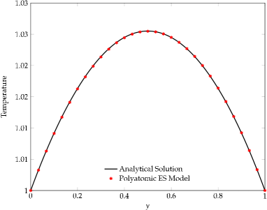
Figure 1: Thermal Couette flow.The temperature distribution along $y$ coordinates in steady state.

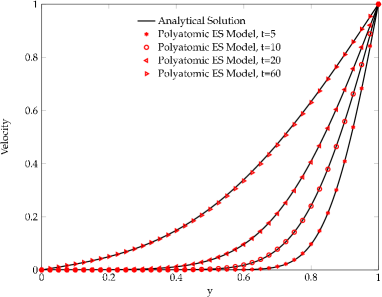
Figure 2: Thermal Couette flow. The velocity distribution along $y$ coordinate at time $t=5$, $t=10$, $t=20$ and $t=60$.

VI.2 The Shock tube flow of 1D

The shock tube problem of one dimension has been discussed extensively in the literature Sod (1978). The initial conditions are given by $(\rho_{L},T_{l},u_{lx})=(4,1,0)$ and $(\rho_{R},T_{r},u_{rx})=(1,1,0)$ on the left and right sides of the shock tube, respectively, where $u_{lx}$ and $u_{rx}$ are the macroscopic velocities along the $x$ coordinate. The specific heat ratio is set as $\gamma=1.4$ and the relaxation time as $\tau=2/3$. The grid is $X\times Y=1000\times 16$, with additional degrees of freedom $N_{f}=3$. The periodic boundary condition is employed for the upper and lower boundaries, while the open boundary condition is used for the left and right boundaries.

The D2Q33 lattice model proposed by J. ShimShim (2013a) is employed. Of all the existing lattice models of fourth-order accuracy, this lattice model has the least discrete velocities, making it more efficient than others. Table 2 gives the discrete velocity set and the weight coefficients of the D2Q33 model.

Table 2: Discrete velocities and weights of D2Q33. $Perm$ denotes permutation and $k$ denotes the number of discrete velocities included in each group. The scaling factor is $r\!=\!0.819381\times\sqrt{2}$.

$k$	$\bm{\xi}_{i}$	$\omega_{i}$
$1$	$(0,0)$	$1.61987e\!-\!1$
$4$	$Perm(r,0)$	$1.43204e\!-\!1$
$4$	$Perm(r,r)$	$3.38840e\!-\!2$
$4$	$Perm(2r,0)$	$5.56112e\!-\!3$
$4$	$Perm(2r,2r)$	$8.44799e\!-\!5$
$4$	$Perm(3r,0)$	$1.13254e\!-\!3$
$8$	$Perm(2r,r)$	$1.28169e\!-\!2$
$4$	$Perm(4r,4r)$	$3.45552e\!-\!6$

Fig. 3 presents the simulation results at $step$ 174, which corresponds to a time of $t=0.15$ when expressed in terms of $\Delta t$, $X$, and $r$. This can be calculated as follows: $t=\frac{step\times\Delta t}{X\times r}=\frac{174\times 1}{1000\times 0.819381\sqrt{2}}\approx 0.15$.

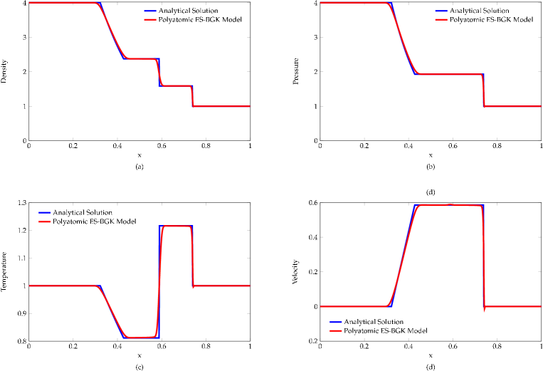
Figure 3: The simulation results of D2Q33 and the analytical resolutions at the time $t\!\approx\!0.15$. The specific heat ratio is $\gamma\!=\!1.4$ and the parameter $N_{f}$ is $3$. The relaxation time is $\tau\!=\!2/3$. The initial condition of the left side is ${\rho\!=\!4,T\!=\!1,\bm{u}\!=\!0}$ and that of the right side is ${\rho\!=\!1,T\!=\!1,\bm{u}\!=\!0}$.

The results are in agreement with the analytical resolutions.

VI.3 A two dimensional supersonic flow on a blunt flat plate

Simulating two-dimensional supersonic flow on a flat blunt plate with an inlet velocity of $u_{inlet}=3\text{Ma}$, the NNDZhang and Zhuang (1991) scheme is used to discretize the advection term of Eq. (30), while the Euler method is employed to discretize the temporal term of Eq. (30).

The velocity boundary condition is applied to the inlet boundary, and the hybrid boundary condition discussed previously is applied to all the walls of the flat plate. The wall density is computed in the same way as the kinetic boundary condition (KBC).The outlet boundary, the upper boundary, and the lower boundary of the entire computational area are set to the zero-gradient boundary condition.

The initial conditions are set as follows: the internal velocity of $\bm{u}=0$, density of $\rho=1$, and temperature of $T=0.71429$, all of which are dimensionless. A computational grid of $200\times 400$ cells is employed, with 60 cells between the front wall of the blunt flat plate and the inlet, 80 cells between the upper wall of the blunt flat plate and the upper boundary of the entire computational area, and the same number of cells between the lower wall of the blunt flat plate and the lower boundary.

The Courant–Friedrichs–Lewy (CFL) principle is employed to determine the time step, with the Courant number set to 0.8. The collision frequency of gas molecules is set to $\gamma=1/6$, and the D2Q37 model discussed previously is utilized.

The pressure configurations at different times are depicted in Fig. (4). In the final figure, the flow becomes stable.

(a)

(b)

(c)

(d)

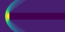
(e)

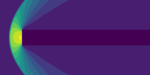
(f)

Figure 4: The pressure configuration of the two-dimensional supersonic flow on a blunt flat plate at various points in time

VII Conclusion

A lattice Boltzmann scheme based on the polyatomic ES-BGK model is proposed, from which the Navier-Stokes equations with an arbitrary Prandtl number and specific heat ratio can be derived via the Chapman-Enskog expansion. The Gaussian distribution is expanded on the Hermite polynomials, and the general term formula for the Hermite coefficients of the Gaussian distribution is deduced, which is the main attribution of this work. To verify the scheme, the thermal Couette flow and the shock tube flow of one dimension are simulated, and the results agree well with the analytical resolutions. A two dimensional supersonic flow on a blunt flat palte is also simulated. The proposed scheme offers a novel way to modify the Prandtl number and the specific heat ratio for the lattice Boltzmann method. As the ES-BGK model satisfies the entropy principle, the lattice Boltzmann scheme proposed in this work can prevent the non-physical results caused by the violation of the $H$-theorem.

Appendix A The derivation of Eq. (27)

The derivation of Eq. (27) is as follows:

$$\bm{a}^{(n)}= \frac{1}{\rho}\int\bm{H}^{(n)}(\bm{u}+\bm{\eta}\cdot\bm{\Lambda}^{\frac{1}{2}})\frac{\rho}{\sqrt{det(2\pi\mathbb{\Lambda})}}$$

$$\times\exp[-\frac{1}{2}(\bm{\xi}-\bm{u})\cdot\bm{\Lambda}^{-1}\cdot(\bm{\xi}-\bm{u})]d(\bm{u}+\bm{\eta}\cdot\bm{\Lambda}^{\frac{1}{2}})$$

$$= \int\bm{H}^{(n)}(\bm{u}+\bm{\eta}\cdot\bm{\Lambda}^{\frac{1}{2}})\omega(\bm{\eta})d\bm{\eta}$$

$$= \sum_{\alpha=0}^{[n/2]}(-1)^{\alpha}\int\omega(\bm{\eta})(\bm{u}+\bm{\eta}\cdot\bm{\Lambda}^{\frac{1}{2}})^{n-2\alpha}\bm{\delta}^{\alpha}d\bm{\eta}$$

$$= \sum_{\alpha=0}^{[n/2]}\sum_{\beta=0}^{[n/2]-\alpha}(-1)^{\alpha}\int\omega(\bm{\eta})\bm{u}^{n-2(\alpha+\beta)}(\bm{\eta}\cdot\bm{\Lambda}^{\frac{1}{2}})^{2\beta}\bm{\delta}^{\alpha}d\bm{\eta}$$

$$= \sum_{\alpha=0}^{[n/2]}\sum_{\beta=0}^{[n/2]-\alpha}(-1)^{\alpha}\bm{u}^{n-2(\alpha+\beta)}\bm{\delta}^{\alpha}[\int\omega(\bm{\eta})\bm{\eta}^{2\beta}d\bm{\eta}\cdot\bm{\Lambda}^{\beta}]$$

$$= \sum_{\alpha=0}^{[n/2]}\sum_{\beta=0}^{[n/2]-\alpha}(-1)^{\alpha}\bm{\delta}^{\alpha}(\bm{\delta}^{\beta}\cdot\bm{\Lambda}^{\beta})\bm{u}^{n-2(\alpha+\beta)}$$

$$= \sum_{\alpha=0}^{[n/2]}\sum_{\beta=0}^{[n/2]-\alpha}(-1)^{\alpha}\bm{\delta}^{\alpha}\bm{\Lambda}^{\beta}\bm{u}^{n-2(\alpha+\beta)}.$$

Appendix B The expansion of Eq. (28)

The expansion of Eq. (28) is as follows:

$$\bm{a}^{(0)}\cdot\bm{H}^{(0)}= 1,$$

$$\bm{a}^{(1)}\cdot\bm{H}^{(1)}= u_{i}\xi_{i},$$

$$\bm{a}^{(2)}\cdot\bm{H}^{(2)}= \Lambda_{ij}\xi_{i}\xi_{j}-\Lambda_{ii}-\xi^{2}+D+(u_{i}\xi_{i})^{2}-u^{2},$$

$$\bm{a}^{(3)}\cdot\bm{H}^{(3)}= 3\Lambda_{ij}\xi_{i}\xi_{j}(u_{i}\xi_{i})$$

$$+3[u^{2}(\Lambda_{ij}\xi_{i}\xi_{j})+2(u_{i}u_{i})(\Lambda_{jk}u_{j}\xi_{k})]$$

$$+(u_{i}\xi_{i})^{3}+3(u_{i}\xi_{i})^{2}\xi^{2}-3(u_{i}\xi_{i})^{2}u^{2}$$

$$-3(D+2)(u_{i}\xi_{i}),$$

$$\bm{a}^{(4)}\cdot\bm{H}^{(4)}= 3\Lambda_{ij}\xi_{i}\xi_{j}-6(\Lambda_{ij}\xi_{i}\xi_{j}$$

$$+2\Lambda_{ik}\xi_{i}\lambda_{jk}\xi_{j})$$

$$+6(\Lambda_{ii}^{2}+2\Lambda_{ij}\Lambda_{ij})$$

$$+6\Lambda_{ij}\xi_{i}\xi_{j}\xi^{2}-6[(D+4)\Lambda_{ij}\xi_{i}\xi_{j}+\Lambda_{ii}\xi^{2}]$$

$$+6(D+2)\Lambda_{ii}+6\Lambda_{ij}\xi_{i}\xi_{j}(u_{k}\xi_{k})^{2}$$

$$-6[\Lambda_{ij}\xi_{i}\xi_{j}u^{2}$$

$$+4\Lambda_{ij}\xi_{i}u_{j}(u_{k}\xi_{k})+\Lambda_{ii}(u_{k}\xi_{k})^{2}]$$

$$+6(\Lambda_{ii}u^{2}+\Lambda_{ij}u_{i}u_{j})$$

$$+(\xi_{i}u_{i})^{4}-6(\xi_{i}u_{i})^{2}u^{2}+3u^{4}$$

$$-6[(\xi_{i}u_{i})^{2}(u^{2}-D-4)+(D+2-u^{2})\xi^{2}]$$

$$+3[u^{4}-2(D+2)u^{2}+D(D+2)].$$

References

• Guo and Zhao (2005) Z. Guo and T. S. Zhao, Physical Review E 71, 026701 (2005).
• Li et al. (2016) Q. Li, K. Luo, Q. Kang, Y. He, Q. Chen,  and Q. Liu, Progress in Energy and Combustion Science 52, 62 (2016).
• Ferreol and Rothman (1995) B. Ferreol and D. H. Rothman, in Multiphase flow in porous media (Springer, 1995) pp. 3–20.
• Chen et al. (2003) H. Chen, S. Kandasamy, S. Orszag, R. Shock, S. Succi,  and V. Yakhot, Science 301, 633 (2003).
• Rahmati and Najjarnezami (2016) A. Rahmati and A. Najjarnezami, Journal of Applied Fluid Mechanics 9, 1201 (2016).
• Yoshino et al. (2004) M. Yoshino, Y. Matsuda,  and C. Shao, International Journal of Computational Fluid Dynamics 18, 333 (2004).
• Kataoka and Tsutahara (2004) T. Kataoka and M. Tsutahara, Physical review E 69, 035701 (2004).
• Watari (2007) M. Watari, Physica A: Statistical Mechanics and its Applications 382, 502 (2007).
• Tsutahara et al. (2008) M. Tsutahara, T. Kataoka, K. Shikata,  and N. Takada, Computers & Fluids 37, 79 (2008).
• Nie et al. (2008) X. Nie, X. Shan,  and H. Chen, Physical Review E 77, 035701 (2008).
• Frapolli et al. (2014) N. Frapolli, S. S. Chikatamarla,  and I. V. Karlin, Physical Review E 90, 043306 (2014).
• Chen et al. (1997) Y. Chen, H. Ohashi,  and M. Akiyama, Journal of scientific computing 12, 169 (1997).
• Yan-Biao et al. (2011) G. Yan-Biao, X. Ai-Guo, Z. Guang-Cai,  and L. Ying-Jun, Communications in Theoretical Physics 56, 490 (2011).
• Soe et al. (1998) M. Soe, G. Vahala, P. Pavlo, L. Vahala,  and H. Chen, Physical Review E 57, 4227 (1998).
• Dellar (2008) P. J. Dellar, Progress in Computational Fluid Dynamics, an International Journal 8, 84 (2008).
• Saadat et al. (2019) M. H. Saadat, F. Bösch,  and I. V. Karlin, Physical Review E 99, 013306 (2019).
• Holway Jr (1965) L. H. Holway Jr, in Rarefied Gas Dynamics, Volume 1, Vol. 1 (1965) p. 193.
• Andries et al. (2000) P. Andries, P. Le Tallec, J.-P. Perlat,  and B. Perthame, European Journal of Mechanics-B/Fluids 19, 813 (2000).
• Andries and Perthame (2001) P. Andries and B. Perthame, in AIP Conference Proceedings (IOP INSTITUTE OF PHYSICS PUBLISHING LTD, 2001) pp. 30–36.
• Andries et al. (2002) P. Andries, J.-F. Bourgat, P. Le Tallec,  and B. Perthame, Computer methods in applied mechanics and engineering 191, 3369 (2002).
• Brull and Schneider (2009) S. Brull and J. Schneider, Continuum Mechanics and Thermodynamics 20, 489 (2009).
• Meng et al. (2013a) J. Meng, Y. Zhang, N. G. Hadjiconstantinou, G. A. Radtke,  and X. Shan, Journal of Fluid Mechanics 718, 347 (2013a).
• Chu (1965a) C. Chu, Physics of Fluids (1958-1988) 8, 12 (1965a).
• Chu (1965b) C. Chu, Physics of Fluids (1958-1988) 8, 1450 (1965b).
• Rykov (1975) V. Rykov, Fluid Dynamics 10, 959 (1975).
• Yudistiawan et al. (2010) W. P. Yudistiawan, S. K. Kwak, D. V. Patil,  and S. Ansumali, Physical Review E 82, 046701 (2010).
• Ansumali et al. (2003) S. Ansumali, I. V. Karlin,  and H. C. Öttinger, EPL (Europhysics Letters) 63, 798 (2003).
• Grad (1949) H. Grad, Communications on Pure and Applied Mathematics 2, 325 (1949).
• Shim and Gatignol (2013) J. W. Shim and R. Gatignol, Zeitschrift für angewandte Mathematik und Physik 64, 473 (2013).
• Mattila et al. (2014a) K. K. Mattila, L. A. Hegele Júnior,  and P. C. Philippi, The Scientific World Journal 2014 (2014a).
• Philippi et al. (2006) P. C. Philippi, L. A. Hegele Jr, L. O. E. Dos Santos,  and R. Surmas, Physical Review E 73, 056702 (2006).
• Philippi et al. (2015) P. Philippi, D. Siebert, L. Hegele Jr,  and K. Mattila, Journal of the Brazilian Society of Mechanical Sciences and Engineering , 1 (2015).
• Shan (2006) X. Shan, Journal of Fluid Mechanics 550, 413 (2006).
• Shan (2010) X. Shan, Physical Review E 81, 036702 (2010).
• Shim (2013a) J. W. Shim, Physical Review E 88, 053310 (2013a).
• Shim (2013b) J. W. Shim, Physical Review E 87, 013312 (2013b).
• Ansumali and Karlin (2002) S. Ansumali and I. V. Karlin, Physical Review E 66, 026311 (2002).
• Sofonea (2009) V. Sofonea, Journal of Computational Physics 228, 6107 (2009).
• Zhao-Li et al. (2002a) G. Zhao-Li, Z. Chu-Guang,  and S. Bao-Chang, Chinese physics 11, 366 (2002a).
• Sod (1978) G. A. Sod, Journal of Computational Physics 27, 1 (1978).
• Zhang and Zhuang (1991) H. Zhang and F. Zhuang, Advances in Applied Mechanics 29, 193 (1991).
• Andries et al. (2000) P. Andries, P. Le Tallec, J.-P. Perlat,  and B. Perthame, Eur. J. Mech., B, Fluids 19, 813 (2000).
• Chen and Doolen (1998) S. Chen and G. D. Doolen, Annual review of fluid mechanics 30, 329 (1998).
• Chen et al. (1992) S. Chen, Z. Wang, X. Shan,  and G. D. Doolen, Journal of Statistical Physics 68, 379 (1992).
• Chikatamarla and Karlin (2009) S. S. Chikatamarla and I. V. Karlin, Physical Review E 79, 046701 (2009).
• Chikatamarla and Karlin (2006) S. S. Chikatamarla and I. V. Karlin, Physical review letters 97, 190601 (2006).
• Jin and Kuznetsov (2017) Y. Jin and A. Kuznetsov, Physics of Fluids 29, 045102 (2017).
• Jin et al. (2015) Y. Jin, M.-F. Uth, A. Kuznetsov,  and H. Herwig, Journal of Fluid Mechanics 766, 76 (2015).
• Mattila et al. (2014b) K. K. Mattila, L. A. Hegele Júnior,  and P. C. Philippi, The Scientific World Journal 2014 (2014b).
• Meng et al. (2013b) J. Meng, L. Wu, J. M. Reese,  and Y. Zhang, Journal of Computational Physics 251, 383 (2013b).
• Shi et al. (2001) W. Shi, W. Shyy,  and R. Mei, Numerical Heat Transfer: Part B: Fundamentals 40, 1 (2001).
• Shim and Gatignol (2011) J. W. Shim and R. Gatignol, Physical Review E 83, 046710 (2011).
• Xu et al. (2014) A. Xu, G. Zhang, Y. Li,  and H. Li, Progress in Physics 34 (2014).
• Zhao-Li et al. (2002b) G. Zhao-Li, Z. Chu-Guang,  and S. Bao-Chang, Chinese Physics 11, 366 (2002b).
• Latt et al. (2020) J. Latt, C. Coreixas, J. Beny,  and A. Parmigiani, Philosophical Transactions of the Royal Society A 378, 20190559 (2020).
• Feng et al. (2009) C. Feng, X. Ai-Guo, Z. Guang-Cai, G. Yan-Biao, C. Tao,  and L. Ying-Jun, Communications in Theoretical Physics 52, 681 (2009).