Simple error bounds for the QBD approximation of a special class of two dimensional reflecting random walks

Keywords: Two-dimensional reflecting random walk (2D-RRW); Double QBD; QBD approximation; Error bound; Time-averaged functional; Geometric ergodicity; Two-node Jackson network with cooperative servers Mathematics Subject Classification: 60J27; 60J22; 60K25.

1 Introduction

This paper considers the stationary distribution of a discrete-time two dimensional reflecting random walk (2D-RRW) on the lattice quarter plane. Such 2D-RRWs appear as the joint queue length processes of two-node queueing systems and two-waiting-line queueing systems. Thus, we can evaluate the long-run performance of these queueing systems once we can obtain the stationary distributions of the corresponding 2D-RRWs.

Unfortunately, it is, in general, difficult to obtain a closed-form expression of the stationary distribution of 2D-RRWs. This is primarily why the tail asymptotics of 2D-RRWs and their generalizations have been extensively studied (see [Boro01, Guil11, Koba13, Koba14, LiHui11, LiHui13, Miya09, Miya11, Miya15, Ozaw13] and the references therein). These studies focus on identifying the decay rate of the stationary distribution, though they make a limited contribution to the performance evaluation of the queueing systems mentioned above.

On the other hand, for some special 2D-RRWs, the product-form solution [Lato14], the mixed-geometric-form solution [Chen15] and the partially geometric solution [Koba15] of the stationary distribution are derived. Although these solutions are tractable and useful, they require restrictive conditions. Thus, the literature [Chen15, Gose14, Lato14] discussed the approximations such that a 2D-RRW is perturbed to another 2D-RRW having the stationary distribution in product form or mixed-geometric form. The studies [Chen15, Gose14] also proposed the linear programming method for establishing error bounds for the linear time-averaged functionals of 2D-RRWs, such as the mean value of the stationary distribution. This linear programming method produces an error bound as a solution of the linear program, and therefore the obtained bound is not explicit.

In fact, it is suggested in [Lato14] that the QBD approximation of 2D-RRWs yields very exact results when the truncation point of the coordinate is sufficiently large. Note that the QBD approximation is such that a 2D-RRW is reduced to a quasi-birth-and-death process (QBD) by truncating one of the two coordinates of the original 2D-RRW. Motivated by this suggestion, we focus on developing computable error bounds for the QBD approximation of 2D-RRWs.

In this paper, we assume some conditions on the mean drifts of the 2D-RRW. Under the conditions, we establish a geometric (Foster-Lyapunov) drift condition on the transition probability matrix of the 2D-RRW. Using the geometric drift condition and the upper bound for the deviation matrix (see, e.g., [Cool02]) of the 2D-RRW, we develop a relative error bound for the approximate time-averaged functional obtained by the QBD approximation. The error bound includes the stationary distribution of the QBD approximation, which can be readily computed by matrix analytic methods (see, e.g., [Lato99]). Thus, the error bound is also computable. In addition, from the error bound, we derive another bound by removing the stationary distribution of the QBD approximation. The second error bound is weaker but simpler than the first one.

2 Preliminaries

In this section, we first introduce the two dimensional reflecting random walk (2D-RRW) and its stability condition. We then describe the technical conditions used to develop our error bounds, while discussing the moment generating functions of the increments of the 2D-RRW. Finally, we establish the geometric drift condition on the 2D-RRW.

2.1 Two dimensional reflecting random walk

Let $\{\bm{Z}(\ell):=(Z_{1}(\ell),Z_{2}(\ell));\ell\in\mathbb{Z}_{+}\}$ denote a two-dimensional Markov chain with state space $\mathbb{S}:=\mathbb{Z}_{+}^{2}=\mathbb{Z}_{+}\times\mathbb{Z}_{+}$, where $\mathbb{Z}_{+}=\{0,1,2,\dots\}$. For $\bm{n}:=(n_{1},n_{2})\in\mathbb{S}$ and $\bm{m}:=(m_{1},m_{2})\in\mathbb{S}$, let $p(\bm{n};\bm{m})$ denote

$$p(\bm{n};\bm{m})=\mathsf{P}(\bm{Z}(\ell+1)=\bm{m}\mid\bm{Z}(\ell)=\bm{n}),\qquad\ell\in\mathbb{Z}_{+}.$$ (2.1)

To describe the behavior of $\{\bm{Z}(\ell)\}$, we introduce some definitions and notation. Let $\mathbb{R}=(-\infty,\infty)$, $\mathbb{Z}=\{0,\pm 1,\pm 2,\dots\}$ and $\mathbb{N}=\{1,2,\dots\}$. Furthermore, let $\mathbb{E}=\{1,2\}$ and $2^{\mathbb{E}}$ denote the power set of $\mathbb{E}$, i.e., $2^{\mathbb{E}}=\{\emptyset,\{1\},\{2\},\mathbb{E}\}$. We then define $\mathbb{S}^{\mathbb{A}}$’s, $\mathbb{A}\in 2^{\mathbb{E}}$, as disjoint subsets of $\mathbb{Z}_{+}^{2}$ such that

$$\mathbb{S}^{\emptyset}=\{(0,0)\},\quad\mathbb{S}^{\{1\}}=\mathbb{N}\times\{0\},\quad\mathbb{S}^{\{2\}}=\{0\}\times\mathbb{N},\quad\mathbb{S}^{\mathbb{E}}=\mathbb{N}^{2}.$$

Clearly, $\cup_{\mathbb{A}\in 2^{\mathbb{E}}}\mathbb{S}^{\mathbb{A}}=\mathbb{S}$. We refer to $\mathbb{S}^{\mathbb{E}}$ and $\mathbb{S}\setminus\mathbb{S}^{\mathbb{E}}$ as the interior and boundary, respectively, of the state space of $\mathbb{S}$. We also refer to $\mathbb{S}^{\emptyset}$, $\mathbb{S}^{\{1\}}$ and $\mathbb{S}^{\{2\}}$ as the boundary faces of the state space $\mathbb{S}$.

For $\mathbb{A}\in 2^{\mathbb{E}}$, let $\bm{X}^{\mathbb{A}}:=(X_{1}^{\mathbb{A}},X_{2}^{\mathbb{A}})$ denote a random vector in $\mathbb{Z}^{2}$ such that $\mathsf{P}(\bm{X}^{\mathbb{A}}\in\mathbb{U}^{\mathbb{A}})=1$, where

$$\mathbb{U}^{\emptyset} =\{0,1\}\times\{0,1\}, \mathbb{U}^{\{1\}} =\{0,\pm 1\}\times\{0,1\},$$

$$\mathbb{U}^{\{2\}} =\{0,1\}\times\{0,\pm 1\}, \mathbb{U}^{\mathbb{E}} =\{0,\pm 1\}\times\{0,\pm 1\}.$$

Furthermore, let $\bm{X}^{\mathbb{A}}(\ell):=(X_{1}^{\mathbb{A}}(\ell),X_{2}^{\mathbb{A}}(\ell))$’s, $\ell\in\mathbb{Z}_{+}$, denote independent copies of $\bm{X}^{\mathbb{A}}$. Thus, for all $\ell\in\mathbb{Z}_{+}$,

$$\mathsf{P}(\bm{X}^{\mathbb{A}}(\ell)=\bm{m})=\mathsf{P}(\bm{X}^{\mathbb{A}}=\bm{m}),\qquad\bm{m}\in\mathbb{Z}^{2}.$$ (2.2)

We now assume that

$$\bm{Z}(\ell+1)=\bm{Z}(\ell)+\sum_{\mathbb{A}\in 2^{\mathbb{E}}}\bm{X}^{\mathbb{A}}(\ell)I(\bm{Z}(\ell)\in\mathbb{S}^{\mathbb{A}}),\qquad\ell\in\mathbb{Z}_{+},$$ (2.3)

where $I(\,\cdot\,)$ denotes the indicator function of the event in the parentheses. We then define $p^{\mathbb{A}}$, $\mathbb{A}\in 2^{\mathbb{E}}$, as the distribution function of $\bm{X}^{\mathbb{A}}$ such that $\sum_{\bm{m}\in\mathbb{U}^{\mathbb{A}}}p^{\mathbb{A}}(\bm{m})=1$ and

$$p^{\mathbb{A}}(\bm{m}) = \mathsf{P}(\bm{X}^{\mathbb{A}}=\bm{m}),\qquad\bm{m}\in\mathbb{Z}^{2}.$$ (2.4)

It follows from (2.2), (2.3) and (2.4) that, for $\bm{n}\in\mathbb{S}^{\mathbb{A}}$ and $\mathbb{A}\in 2^{\mathbb{E}}$,

$$\mathsf{P}(\bm{Z}(\ell+1)=\bm{n}+\bm{m}\mid\bm{Z}(\ell)=\bm{n}) = p^{\mathbb{A}}(\bm{m}),\qquad\bm{m}\in\mathbb{Z}^{2}.$$ (2.5)

It also follows from (2.1), (2.5) and $\sum_{\bm{m}\in\mathbb{U}^{\mathbb{A}}}p^{\mathbb{A}}(\bm{m})=1$ that

$$p(\bm{n};\bm{m})=p^{\mathbb{A}}(\bm{m}-\bm{n}),\quad\bm{n}\in\mathbb{S}^{\mathbb{A}},\ \bm{m}-\bm{n}\in\mathbb{U}^{\mathbb{A}},\ \mathbb{A}\in 2^{\mathbb{E}}.$$ (2.6)

In what follows, we refer to $\{\bm{Z}(\ell)\}$ described above as a two dimensional reflecting random walk (2D-RRW). We also refer to $p^{\mathbb{A}}$ and $\{\bm{X}^{\mathbb{A}}(\ell)\}$ as the transition law and increment, respectively, in $\mathbb{S}^{\mathbb{A}}$.

2.2 Stability condition

In this subsection, we provide the summary of the known results on the stability condition (ergodic condition) of the 2D-RRW $\{\bm{Z}(\ell)\}$.

For $\mathbb{A}\in 2_{+}^{\mathbb{E}}:=\{\{1\},\{2\},\mathbb{E}\}$, let

$$\bm{\mu}^{\mathbb{A}}:=(\mu_{1}^{\mathbb{A}},\mu_{2}^{\mathbb{A}})=(\mathsf{E}[X^{\mathbb{A}}_{1}],\mathsf{E}[X^{\mathbb{A}}_{2}]).$$ (2.7)

It follows from (2.3) that $\bm{\mu}^{\mathbb{A}}$ is the vector of the mean increments of the 2D-RRW $\{\bm{Z}(\ell)\}$ in $\mathbb{S}^{\mathbb{A}}$. Thus, we call $\bm{\mu}^{\mathbb{A}}$ the mean drift in $\mathbb{S}^{\mathbb{A}}$. By definition, $X_{2}^{\{1\}}\geq 0$ and $X_{1}^{\{2\}}\geq 0$ with probability one (w.p.1), which leads to

$$\mu_{2}^{\{1\}}\geq 0,\qquad\mu_{1}^{\{2\}}\geq 0.$$ (2.8)

In addition, for any two vectors $\bm{x}=(x_{1},x_{2})$ and $\bm{y}=(y_{1},y_{2})$ in $\mathbb{R}^{2}$, let

$$\bm{x}\wedge\bm{y}=x_{1}y_{2}-x_{2}y_{1}.$$

Note here that $\bm{x}\wedge\bm{y}$ is equivalent to the third element of the cross product of two vectors $(\bm{x},0)$ and $(\bm{y},0)$ in $\mathbb{R}^{3}$. Therefore, $\bm{x}\wedge\bm{y}>0$ (resp. $\bm{x}\wedge\bm{y}<0$) if and only if the direction angle of vector $\bm{y}$ from vector $\bm{x}$ is in the range $(0,\pi)$ (resp. $(-\pi,0)$), where the positive direction is counterclockwise.

In the rest of this paper, we assume that the 2D-RRW $\{\bm{Z}(\ell)\}$ is irreducible and aperiodic. We also assume the following stability condition of the 2D-RRW $\{\bm{Z}(\ell)\}$.

Assumption 2.1 (Stability condition)

Either of the following is satisfied:

1. $\mu_{1}^{\mathbb{E}}<0$, $\mu_{2}^{\mathbb{E}}<0$, $\bm{\mu}^{\mathbb{E}}\wedge\bm{\mu}^{\{1\}}<0$ and $\bm{\mu}^{\mathbb{E}}\wedge\bm{\mu}^{\{2\}}>0$.

2. $\mu_{1}^{\mathbb{E}}\geq 0$, $\mu_{2}^{\mathbb{E}}<0$ and $\bm{\mu}^{\mathbb{E}}\wedge\bm{\mu}^{\{1\}}<0$. In addition, $\mu^{\{2\}}_{2}<0$ if $\mu^{\{2\}}_{1}=0$.

3. $\mu_{1}^{\mathbb{E}}<0$, $\mu_{2}^{\mathbb{E}}\geq 0$ and $\bm{\mu}^{\mathbb{E}}\wedge\bm{\mu}^{\{2\}}>0$. In addition, $\mu^{\{1\}}_{1}<0$ if $\mu^{\{1\}}_{2}=0$.

It is known (see, e.g., [Koba13]) that if Assumption 2.1 holds then the 2D-RRW $\{\bm{Z}(\ell)\}$ has the unique stationary distribution, denoted by $\bm{\pi}:=(\pi(n_{1},n_{2}))_{(n_{1},n_{2})\in\mathbb{S}}$. The geometric interpretation of this stability condition is summarized in Figs. 1(a), 1(b) and 1(c).

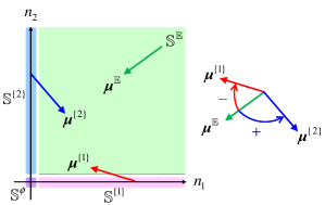
(a) Case (a)

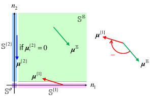
(b) Case (b)

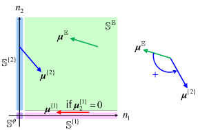
(c) Case (c)

Figure 1: Stability condition

Remark 2.1

Provided $\bm{\mu}^{\mathbb{E}}\neq\bm{0}$, Assumption 2.1 holds if and only if the 2D-RRW $\{\bm{Z}(\ell)\}$ has the unique stationary distribution. It is known that, even if $\bm{\mu}^{\mathbb{E}}=\bm{0}$, the 2D-RRW $\{\bm{Z}(\ell)\}$ can be stable though its stationary distribution must be heavy-tailed. For details, see [Fayo95, Koba14].

2.3 Moment generating functions of increments

In this subsection, we discuss the moment generating functions of the increments $\bm{X}^{\mathbb{A}}$’s and describe the technical conditions used to obtain the main results of this paper.

Let $\gamma^{\mathbb{A}}$, $\mathbb{A}\in 2_{+}^{\mathbb{E}}$, denote the moment generating function of $\bm{X}^{\mathbb{A}}$, i.e.,

$$\gamma^{\mathbb{A}}(\bm{\theta})=\mathsf{E}[\exp\{\langle\bm{\theta},\bm{X}^{\mathbb{A}}\rangle\}],\quad\bm{\theta}:=(\theta_{1},\theta_{2})\in\mathbb{R}^{2},$$ (2.9)

where $\langle\bm{x},\bm{y}\rangle$ denotes the inner product of vectors $\bm{x}$ and $\bm{y}$. From (2.7) and (2.9), we have

$$\mu_{a}^{\mathbb{A}}=\mathsf{E}[X_{a}^{\mathbb{A}}]={\partial\gamma^{\mathbb{A}}\over\partial\theta_{a}}(\bm{0}),\qquad\mathbb{A}\in 2_{+}^{\mathbb{E}},\ a\in\{1,2\}.$$ (2.10)

Furthermore, let $\mathsf{\mathsf{\Gamma}}^{\mathbb{A}}$ and $\partial\mathsf{\Gamma}^{\mathbb{A}}$, $\mathbb{A}\in 2_{+}^{\mathbb{E}}$, denote

$$\mathsf{\Gamma}^{\mathbb{A}}=\{\bm{\theta};\gamma^{\mathbb{A}}(\bm{\theta})<1\},\quad\partial\mathsf{\Gamma}^{\mathbb{A}}=\{\bm{\theta};\gamma^{\mathbb{A}}(\bm{\theta})=1\},$$ (2.11)

respectively.

Under Assumption 2.1, we have the following propositions (see [Koba14, Remark 2 and Lemma 2]).

Proposition 2.1

If Assumption 2.1 holds, then the following are true:

1. For each $\mathbb{A}\in 2_{+}^{\mathbb{E}}$, $\mathsf{\Gamma}^{\mathbb{A}}$ is a convex set and $\bm{0}\in\partial\mathsf{\Gamma}^{\mathbb{A}}$.

2. $\mathsf{\Gamma}^{\mathbb{E}}\cap\mathbb{R}_{>0}^{2}\neq\emptyset$, where $\mathbb{R}_{>0}=\{x\in\mathbb{R}:x>0\}=(0,\infty)$.

Proposition 2.2

Assumption 2.1 holds if and only if, for each $a\in\{1,2\}$, there exists some $\bm{\theta}\in\partial\mathsf{\Gamma}^{\mathbb{E}}\cap\partial\mathsf{\Gamma}^{\{a\}}$ such that $\theta_{a}>0$.

Remark 2.2

The symbol “$\partial$” is dropped in the original statement of [Koba14, Lemma 2].

We now present a geometric property of $\mathsf{\Gamma}^{\{1\}}$ and $\mathsf{\Gamma}^{\{2\}}$.

Lemma 2.1

Suppose that Assumption 2.1 holds. For each $a\in\{1,2\}$, $\mu_{a}^{\{a\}}<0$ if and only if $\mathsf{\Gamma}^{\{a\}}\cap\mathbb{R}_{>0}^{2}\neq\emptyset$.

Proof.   We fix $a\in\{1,2\}$ arbitrarily. Since $|X_{1}^{\{a\}}|=|X_{2}^{\{a\}}|\leq 1$, the moment generating function $\gamma^{\{a\}}(\bm{\theta})$ is holomorphic at $\bm{\theta}=\bm{0}$. It thus follows from the Taylor’s expansion of $\gamma^{\{a\}}(\bm{\theta})$ at $\bm{\theta}=\bm{0}$ that the following holds at a neighborhood of $\bm{\theta}=\bm{0}$:

$$\gamma^{\{a\}}(\bm{\theta})=\gamma^{\{a\}}(\bm{0})+\langle(\nabla_{\!\bm{\theta}}\gamma^{\{a\}})(\bm{0}),\bm{\theta}\rangle+o(\|\bm{\theta}\|^{2}),$$ (2.12)

where $\|\cdot\|$ denotes an arbitrary norm on $\mathbb{R}^{2}$, and where $\nabla_{\!\bm{\theta}}$ denotes the gradient operator with respect to a vector variable $\bm{\theta}$, i.e.,

$$\nabla_{\!\bm{\theta}}=\left({\partial\over\partial\theta_{1}},{\partial\over\partial\theta_{2}}\right).$$

Furthermore, it follows from (2.10) that

$$(\nabla_{\!\bm{\theta}}\gamma^{\{a\}})(\bm{0})=\left({\partial\gamma^{\{a\}}\over\partial\theta_{1}}(\bm{0}),{\partial\gamma^{\{a\}}\over\partial\theta_{2}}(\bm{0}),\right)=(\mu_{1}^{\{a\}},\mu_{2}^{\{a\}}).$$

Substituting this equation and $\gamma^{\{a\}}(\bm{0})=1$ into (2.12) yields

$$\gamma^{\{a\}}(\bm{\theta})-1=\mu_{1}^{\{a\}}\theta_{1}+\mu_{2}^{\{a\}}\theta_{2}+o(\|\bm{\theta}\|^{2}),$$

which implies that $\mathsf{\Gamma}^{\{a\}}\cap\mathbb{R}_{>0}^{2}\neq\emptyset$ if and only if $\mu_{1}^{\{a\}}\theta_{1}+\mu_{2}^{\{a\}}\theta_{2}<0$ for some $\bm{\theta}>\bm{0}$, or equivalently, either $\mu_{1}^{\{a\}}<0$ or $\mu_{2}^{\{a\}}<0$. Recall here that $\mu_{3-a}^{\{a\}}\geq 0$ due to (2.8). As a result, $\mu_{a}^{\{a\}}<0$ if and only if $\mathsf{\Gamma}^{\{a\}}\cap\mathbb{R}_{>0}^{2}\neq\emptyset$. $\Box$

We now introduce the following assumption (see Fig. 2).

Assumption 2.2

$\mu_{1}^{\{1\}}<0$, $\mu_{2}^{\{2\}}<0$ and

$$\bm{\mu}^{\{1\}}\wedge\bm{\mu}^{\{2\}}=\mu_{1}^{\{1\}}\mu_{2}^{\{2\}}-\mu_{2}^{\{1\}}\mu_{1}^{\{2\}}>0.$$ (2.13)

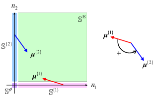
Figure 2: Mean drifts satisfying Assumption 2.2

Remark 2.3

Recall that $\mu_{2}^{\{1\}}\geq 0$ and $\mu_{1}^{\{2\}}\geq 0$, as shown in (2.8). If either $\mu_{2}^{\{1\}}=0$ or $\mu_{1}^{\{2\}}=0$ holds, then (2.13) follows from $\mu_{1}^{\{1\}}<0$ and $\mu_{2}^{\{2\}}<0$.

Remark 2.4

A typical example of 2D-RRWs satisfying Assumption 2.2 is a two-node Jackson network with cooperative servers. For details, see Appendix LABEL:appendix-Jackson.

From Lemma 2.1, we have the following result, which plays an important role in the next section.

Lemma 2.2

Assumption 2.2 holds if and only if

$$\bigcap_{\mathbb{A}\in 2_{+}^{\mathbb{E}}}\mathsf{\Gamma}^{\mathbb{A}}\cap\mathbb{R}^{2}_{>0}=\mathsf{\Gamma}^{\{1\}}\cap\mathsf{\Gamma}^{\{2\}}\cap\mathsf{\Gamma}^{\mathbb{E}}\cap\mathbb{R}^{2}_{>0}\neq\emptyset,$$ (2.14)

provided that Assumption 2.1 is satisfied.

Proof.   Lemma 2.1 shows that Assumption 2.2 is necessary for that $\bigcap_{\mathbb{A}\in 2_{+}^{\mathbb{E}}}\mathsf{\Gamma}^{\mathbb{A}}\cap\mathbb{R}^{2}_{>0}\neq\emptyset$. It follows from (2.9) and (2.11) that the domains $\mathsf{\Gamma}^{\mathbb{A}}\cup\partial\mathsf{\Gamma}^{\mathbb{A}}$’s, $\mathbb{A}\in 2_{+}^{\mathbb{E}}$, are convex and the curves $\partial\mathsf{\Gamma}^{\mathbb{A}}$’s, $\mathbb{A}\in 2_{+}^{\mathbb{E}}$, include the origin $(0,0)$. Furthermore, $\bm{\mu}^{\{1\}}$ and $\bm{\mu}^{\{2\}}$ are the gradient vectors, at the origin $(0,0)$, of the functions $\gamma^{\{1\}}$ and $\gamma^{\{2\}}$, respectively and they satisfy (2.8). These facts, together with Fig. 3, imply that if $\bm{\mu}^{\{1\}}\wedge\bm{\mu}^{\{2\}}>0$ then $\bigcap_{\mathbb{A}\in 2_{+}^{\mathbb{E}}}\mathsf{\Gamma}^{\mathbb{A}}\cap\mathbb{R}^{2}_{>0}\cap\mathbb{R}^{2}_{>0}\neq\emptyset$, and vice versa. As a result, Assumption 2.2 is equivalent to (2.14), under Assumption 2.1. $\Box$

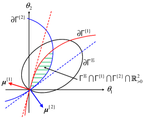
Figure 3: Relation between the domains $\mathsf{\Gamma}^{\mathbb{E}}$, $\mathsf{\Gamma}^{\{1\}}$ and $\mathsf{\Gamma}^{\{2\}}$

2.4 Geometric drift condition

In this subsection, we show that a Foster-Lyapunov condition (Condition 2.1 below) holds for the transition probability matrix $\bm{P}:=(p(\bm{n};\bm{m}))_{(\bm{n};\bm{m})\in\mathbb{S}^{2}}$ of the 2D-RRW $\{\bm{Z}(\ell)\}$ (see (2.1)), under Assumptions 2.1 and 2.2.

Condition 2.1 ([Meyn09, Section 14.2.1])

There exist a finite set $\mathbb{K}\subset\mathbb{S}$, $b\in\mathbb{R}_{>0}$, $c\in(0,1)$ and column vector $\bm{v}:=(v(\bm{n}))_{\bm{n}\in\mathbb{S}}\geq\bm{e}/c$ such that

$$\bm{P}\bm{v}-\bm{v}\leq-c\bm{v}+b\bm{1}_{\mathbb{K}},$$ (2.15)

where, for any set $\mathbb{C}\subseteq\mathbb{S}$, $\bm{1}_{\mathbb{C}}:=(1_{\mathbb{C}}(\bm{n}))_{\bm{n}\in\mathbb{S}}$ denotes a column vector such that

$$1_{\mathbb{C}}(\bm{n})=\left\{\begin{array}[]{ll}1,&\bm{n}\in\mathbb{C},\\ 0,&\bm{n}\in\mathbb{S}\setminus\mathbb{C}.\end{array}\right.$$

It is known ([Meyn09, Theorem 15.0.1]) that if $\bm{P}$ is irreducible and aperiodic and Condition 2.1 holds then $\bm{P}$ is geometrically ergodic. Thus, we refer to Condition 2.1 as the geometric drift condition.

Under Assumptions 2.1 and 2.2, we establish the geometric drift condition on the 2D-RRW.

Lemma 2.3

Suppose that Assumptions 2.1 and 2.2 are satisfied. Fix $\bm{\theta}\in\bigcap_{\mathbb{A}\in 2_{+}^{\mathbb{E}}}\mathsf{\Gamma}^{\mathbb{A}}\cap\mathbb{R}_{>0}^{2}$ and $\bm{v}=(v(\bm{n}))_{\bm{n}\in\mathbb{S}}$ such that

$$v(\bm{n})=c^{-1}\exp\{\langle\bm{\theta},\bm{n}\rangle\},\qquad\bm{n}\in\mathbb{S},$$ (2.16)

where

$$c=1-\max(\gamma^{\{1\}}(\bm{\theta}),\gamma^{\{2\}}(\bm{\theta}),\gamma^{\mathbb{E}}(\bm{\theta})).$$ (2.17)

Under these conditions, Condition 2.1 holds for $\mathbb{K}=\{(0,0)\}$ and

$$b=1+c^{-1}(\gamma^{\emptyset}(\bm{\theta})-1)>0.$$ (2.18)

Proof.  It follows from (2.9) and (2.16) that, for $\bm{n}\in\mathbb{S}^{\mathbb{A}}$ and $\mathbb{A}\in 2_{+}^{\mathbb{E}}$,

$$\sum_{\bm{m}\in\mathbb{U}^{\mathbb{A}}}p^{\mathbb{A}}(\bm{m})v(\bm{n}+\bm{m}) = c^{-1}\sum_{\bm{m}\in\mathbb{U}^{\mathbb{A}}}p^{\mathbb{A}}(\bm{m})\exp\{\langle\bm{\theta},\bm{n}+\bm{m}\rangle\}$$

$$= c^{-1}\exp\{\langle\bm{\theta},\bm{n}\rangle\}\sum_{\bm{m}\in\mathbb{U}^{\mathbb{A}}}p^{\mathbb{A}}(\bm{m})\exp\{\langle\bm{\theta},\bm{m}\rangle\}$$

$$= v(\bm{n})\gamma^{\mathbb{A}}(\bm{\theta})\leq(1-c)v(\bm{n}),$$

where the inequality is due to (2.17). Similarly, we have

$$\sum_{\bm{m}\in\mathbb{U}^{\emptyset}}p^{\emptyset}(\bm{m})v(\bm{m}) = c^{-1}\sum_{\bm{m}\in\mathbb{U}^{\emptyset}}p^{\emptyset}(\bm{m})\exp\{\langle\bm{\theta},\bm{m}\rangle\}$$

$$= c^{-1}\gamma^{\emptyset}(\bm{\theta})=(c^{-1}-1)+b$$

$$= (1-c)v(\bm{0})+b,$$

where the last two equalities are due to (2.18) and $v(\bm{0})=c^{-1}$. Note here that, since $\bm{\theta}>\bm{0}$ and $\bm{X}^{\emptyset}\geq\bm{0}$, we have $\gamma^{\emptyset}(\bm{\theta})-1\geq 0$ and thus $b>0$. Therefore, (2.15) holds for $\mathbb{K}=\{(0,0)\}$ and $b$ given in (2.18). $\Box$

3 QBD approximation

This section describes the QBD approximation of the 2D-RRW $\{\bm{Z}(\ell);\ell\in\mathbb{Z}_{+}\}$. We first reformulate the 2D-RRW $\{\bm{Z}(\ell)\}$ as a quasi-birth-and-death process (QBD) such that its phase process is an infinite birth-and-death process. We then provide the definition of the QBD approximation of the 2D-RRW.

3.1 Reformulation as double QBD

For convenience, we refer to $Z_{1}(\ell)$ and $Z_{2}(\ell)$ as the level and the phase, respectively. We then arrange the elements of the state space $\mathbb{S}$ in a lexicographical order such that the level is the primary variable and the phase is the secondary one. Since the marginal processes $\{Z_{1}(\ell)\}$ and $\{Z_{2}(\ell)\}$ increases or decreases by at most one, the transition probability matrix $\bm{P}$ of $\{\bm{Z}(\ell)\}$ has the QBD-structure:

$$\bm{P}=\left(\begin{array}[]{@{}c@{~}c@{~}c@{~}c@{~}c@{~}c@{}}\bm{B}(0)\hfil~{}&\bm{B}(1)\hfil~{}&\bm{O}\hfil~{}&\bm{O}\hfil~{}&\bm{O}\hfil~{}&\cdots\\ \bm{A}(-1)\hfil~{}&\bm{A}(0)\hfil~{}&\bm{A}(1)\hfil~{}&\bm{O}\hfil~{}&\bm{O}\hfil~{}&\cdots\\ \bm{O}\hfil~{}&\bm{A}(-1)\hfil~{}&\bm{A}(0)\hfil~{}&\bm{A}(1)\hfil~{}&\bm{O}\hfil~{}&\cdots\\ \bm{O}\hfil~{}&\bm{O}\hfil~{}&\bm{A}(-1)\hfil~{}&\bm{A}(0)\hfil~{}&\bm{A}(1)\hfil~{}&\cdots\\ \vdots\hfil~{}&\vdots\hfil~{}&\vdots\hfil~{}&\vdots\hfil~{}&\ddots\hfil~{}&\ddots\end{array}\right),$$ (3.6)

where $\bm{O}$ denotes the zero matrix, and where $\bm{A}(k)$, $k\in\{0,\pm 1\}$, and $\bm{B}(k)$, $k\in\{0,1\}$, are given by

$$\bm{A}(k) =\left(\begin{array}[]{@{}c@{~\,}c@{~\,}c@{~\,}c@{~\,}c@{}}p^{\{1\}}(k,0)\hfil~{}&p^{\{1\}}(k,1)\hfil~{}&0\hfil~{}&0\hfil~{}&\cdots\\ p^{\mathbb{E}}(k,-1)\hfil~{}&p^{\mathbb{E}}(k,0)\hfil~{}&p^{\mathbb{E}}(k,1)\hfil~{}&0\hfil~{}&\cdots\\ 0\hfil~{}&p^{\mathbb{E}}(k,-1)\hfil~{}&p^{\mathbb{E}}(k,0)\hfil~{}&p^{\mathbb{E}}(k,1)\hfil~{}&\cdots\\ 0\hfil~{}&0\hfil~{}&p^{\mathbb{E}}(k,-1)\hfil~{}&p^{\mathbb{E}}(k,0)\hfil~{}&\cdots\\ \vdots\hfil~{}&\vdots\hfil~{}&\vdots\hfil~{}&\vdots\hfil~{}&\ddots\end{array}\right),$$ (3.12)

and

$$\bm{B}(k) =\left(\begin{array}[]{@{}c@{~}c@{~}c@{~}c@{~}c@{}}p^{\emptyset}(k,0)\hfil~{}&p^{\emptyset}(k,1)\hfil~{}&0\hfil~{}&0\hfil~{}&\cdots\\ \rule{0.0pt}{14.22636pt}p^{\{2\}}(k,-1)\hfil~{}&p^{\{2\}}(k,0)\hfil~{}&p^{\{2\}}(k,1)\hfil~{}&0\hfil~{}&\cdots\\ \rule{0.0pt}{14.22636pt}0\hfil~{}&p^{\{2\}}(k,-1)\hfil~{}&p^{\{2\}}(k,0)\hfil~{}&p^{\{2\}}(k,1)\hfil~{}&\cdots\\ \rule{0.0pt}{14.22636pt}0\hfil~{}&0\hfil~{}&p^{\{2\}}(k,-1)\hfil~{}&p^{\{2\}}(k,0)\hfil~{}&\cdots\\ \rule{0.0pt}{14.22636pt}\vdots\hfil~{}&\vdots\hfil~{}&\vdots\hfil~{}&\vdots\hfil~{}&\ddots\end{array}\right),$$ (3.18)

respectively. By interchanging $Z_{1}(\ell)$ and $Z_{2}(\ell)$, we can construct another QBD-structured transition probability matrix. This is why the reformulated $\{\bm{Z}(\ell)\}$ is sometimes called a double QBD [Koba13, Miya09].

3.2 Definition of QBD approximation

For $n\in\mathbb{Z}_{+}$, let $\hskip 1.00006pt{}_{[n]}\bm{A}(k):=(\hskip 1.00006pt{}_{[n]}A_{i,j}(k))_{i,j\in\mathbb{Z}_{n}}$, $k\in\{0,\pm 1\}$, and $\hskip 1.00006pt{}_{[n]}\bm{B}(k):=(\hskip 1.00006pt{}_{[n]}B_{i,j}(k))_{i,j\in\mathbb{Z}_{n}}$, $k\in\{0,1\}$, denote

$$\hskip 1.00006pt{}_{[n]}\bm{A}(k)=\left(\begin{array}[]{@{}c@{}c@{}c@{~}|@{~}c@{}}&&\hfil~{}\vrule~{}&0\\ &\hskip 1.00006pt{}_{(n-1)}\bm{A}(k)&\hfil~{}\vrule~{}&\vdots\\ &&\hfil~{}\vrule~{}&0\\ &&\hfil~{}\vrule~{}&p^{\mathbb{E}}(k,1)\\ \hline\cr 0&\cdots&0~{}~{}p^{\mathbb{E}}(k,-1)\hfil~{}\vrule~{}&\rule{0.0pt}{14.22636pt}\displaystyle\sum_{i=0}^{1}p^{\mathbb{E}}(k,i)\end{array}\right),$$ (3.19)

and

$$\hskip 1.00006pt{}_{[n]}\bm{B}(k)=\left(\begin{array}[]{@{}c@{}c@{}c@{~}|@{~}c@{}}&&\hfil~{}\vrule~{}&0\\ &\hskip 1.00006pt{}_{(n-1)}\bm{B}(k)&\hfil~{}\vrule~{}&\vdots\\ &&\hfil~{}\vrule~{}&0\\ &&\hfil~{}\vrule~{}&p^{\{2\}}\!(k,1)\\ \hline\cr 0&\cdots&0~{}~{}p^{\{2\}}\!(k,-1)\hfil~{}\vrule~{}&\rule{0.0pt}{14.22636pt}\displaystyle\sum_{i=0}^{1}p^{\{2\}}\!(k,i)\end{array}\right).$$ (3.20)

respectively, where $\mathbb{Z}_{n}=\{0,1,\dots,n\}$, and where $\hskip 1.00006pt{}_{(n)}\bm{A}(k):=(\hskip 1.00006pt{}_{(n)}A_{i,j}(k))_{i,j\in\mathbb{Z}_{n}}$ and $\hskip 1.00006pt{}_{(n)}\bm{B}(k):=(\hskip 1.00006pt{}_{(n)}B_{i,j}(k))_{i,j\in\mathbb{Z}_{n}}$ are the $(n+1)\times(n+1)$ northwest-corners of $\bm{A}(k)$ and $\bm{B}(k)$, respectively. We then define $\hskip 1.00006pt{}_{[n]}\bm{P}:=(\hskip 1.00006pt{}_{[n]}p(k,i;k^{\prime},i^{\prime}))_{(k,i;k^{\prime},i^{\prime})\in(\mathbb{Z}_{+}\times\mathbb{Z}_{n})^{2}}$, $n\in\mathbb{N}$, as

$$\hskip 1.00006pt{}_{[n]}\bm{P}=\left(\begin{array}[]{@{}c@{\,}c@{\,}c@{\,}c@{\,}c@{}}\hskip 1.00006pt{}_{[n]}\bm{B}(0)&\hskip 1.00006pt{}_{[n]}\bm{B}(1)&\bm{O}&\bm{O}&\cdots\\ \hskip 1.00006pt{}_{[n]}\bm{A}(-1)&\hskip 1.00006pt{}_{[n]}\bm{A}(0)&\hskip 1.00006pt{}_{[n]}\bm{A}(1)&\bm{O}&\cdots\\ \bm{O}&\hskip 1.00006pt{}_{[n]}\bm{A}(-1)&\hskip 1.00006pt{}_{[n]}\bm{A}(0)&\hskip 1.00006pt{}_{[n]}\bm{A}(1)&\cdots\\ \bm{O}&\bm{O}&\hskip 1.00006pt{}_{[n]}\bm{A}(-1)&\hskip 1.00006pt{}_{[n]}\bm{A}(0)&\cdots\\ \vdots&\vdots&\vdots&\vdots&\ddots\end{array}\right),$$ (3.21)

where $(k,i;k^{\prime},i^{\prime})$ denotes ordered pair $((k,i),(k^{\prime},i^{\prime}))$ in $(\mathbb{Z}_{+}\times\mathbb{Z}_{n})^{2}$. Clearly, $\hskip 1.00006pt{}_{[n]}\bm{P}$ is the transition probability matrix of a standard QBD, i.e., a QBD with infinite levels and finite phases. Thus, we refer to $\hskip 1.00006pt{}_{[n]}\bm{P}$ as the QBD approximation to $\bm{P}$.

We now consider a two-dimensional Markov chain $\{\hskip 1.00006pt{}_{[n]}\bm{Z}(\ell):=(\hskip 1.00006pt{}_{[n]}Z_{1}(\ell),\hskip 1.00006pt{}_{[n]}Z_{2}(\ell));\ell\in\mathbb{Z}_{+}\}$ with state space $\mathbb{S}_{n}:=\mathbb{Z}_{+}\times\mathbb{Z}_{n}$ such that

$$\hskip 1.00006pt{}_{[n]}Z_{1}(\ell+1) =\hskip 1.00006pt{}_{[n]}Z_{1}(\ell)+\sum_{\mathbb{A}\in 2^{\mathbb{E}}}X_{1}^{\mathbb{A}}(\ell)I(\hskip 1.00006pt{}_{[n]}\bm{Z}(\ell)\in\mathbb{S}^{\mathbb{A}}), \ell \in\mathbb{Z}_{+},$$ (3.22)

$$\hskip 1.00006pt{}_{[n]}Z_{2}(\ell+1) =\min\!\bigg{(}n,\hskip 1.00006pt{}_{[n]}Z_{2}(\ell)+\sum_{\mathbb{A}\in 2^{\mathbb{E}}}X_{2}^{\mathbb{A}}(\ell)I(\hskip 1.00006pt{}_{[n]}\bm{Z}(\ell)\in\mathbb{S}^{\mathbb{A}})\bigg{)}, \ell \in\mathbb{Z}_{+}.$$ (3.23)

It is easy to see that $\hskip 1.00006pt{}_{[n]}\bm{P}$ is equal to the transition probability matrix of the two-dimensional Markov chain $\{\hskip 1.00006pt{}_{[n]}\bm{Z}(\ell)\}$. Note here that $\{\hskip 1.00006pt{}_{[n]}\bm{Z}(\ell)\}$ is a 2D-RRW obtained by adding a reflecting barrier at $n_{2}=n$ to the state space $\mathbb{S}=\{(n_{1},n_{2})\in\mathbb{Z}_{+}^{2}\}$ of the original 2D-RRW $\{\bm{Z}(\ell)\}$. Since $\{\bm{Z}(\ell)\}$ is ergodic (i.e., irreducible, positive recurrent and aperiodic), it follows from (3.22) and (3.23) that $\{\hskip 1.00006pt{}_{[n]}\bm{Z}(\ell)\}$ is irreducible and positive recurrent. Therefore, $\hskip 1.00006pt{}_{[n]}\bm{P}$ has the unique stationary distribution, denoted by $\hskip 1.00006pt{}_{[n]}\bm{\pi}:=(\hskip 1.00006pt{}_{[n]}\pi((k,i))_{(k,i)\in\mathbb{S}_{n}}$, which is referred to as the QBD approximation to $\bm{\pi}$.

4 Error bounds for QBD approximation

In this section, we assume that Assumptions 2.1 and 2.2 hold, under which we present relative error bounds for the approximate time-averaged functional obtained by the QBD approximation $\hskip 1.00006pt{}_{[n]}\bm{\pi}$.

For each $n\in\mathbb{Z}_{+}$, we extend $\hskip 1.00006pt{}_{[n]}\bm{\pi}$, $\hskip 1.00006pt{}_{[n]}\bm{A}(k)$ and $\hskip 1.00006pt{}_{[n]}\bm{B}(k)$ to the respective orders of $\bm{\pi}$, $\bm{A}(k)$ and $\bm{B}(k)$ in such a way that

$$\hskip 1.00006pt{}_{[n]}\pi(k,i) =0, k \in\mathbb{Z}_{+}, i \in\mathbb{Z}_{+}\setminus\mathbb{Z}_{n},$$ (4.1)

$$\hskip 1.00006pt{}_{[n]}A_{i,j}(k) =0, k \in\{0,\pm 1\}, (i,j) \in\mathbb{S}\setminus\mathbb{Z}_{n}^{2},$$ (4.2)

$$\hskip 1.00006pt{}_{[n]}B_{i,j}(k) =0, k \in\{0,1\}, (i,j) \in\mathbb{S}\setminus\mathbb{Z}_{n}^{2}.$$ (4.3)

Therefore, $\hskip 1.00006pt{}_{[n]}\bm{P}$ is of the same order as that of $\bm{P}$.

We now define $\bm{D}$ as the deviation matrix of $\bm{P}$ (see, e.g., [Cool02]), i.e.,

$$\bm{D}=\sum_{\ell=0}^{\infty}(\bm{P}^{\ell}-\bm{e}\bm{\pi}).$$ (4.4)

Since $\bm{P}$ is geometrically ergodic (see Condition 2.1 and Lemma 2.3), the deviation matrix $\bm{D}$ is well-defined (see, e.g., [Meyn09, Theorem 15.0.1]). Furthermore, combining [Heid10, Section 4.1, Equation (9)] together with (4.1)–(4.3) yields

$$\hskip 1.00006pt{}_{[n]}\bm{\pi}-\bm{\pi}=\hskip 1.00006pt{}_{[n]}\bm{\pi}\left(\hskip 1.00006pt{}_{[n]}\bm{P}-\bm{P}\right)\bm{D},\qquad n\in\mathbb{N},$$

which leads to

$$|\hskip 1.00006pt{}_{[n]}\bm{\pi}-\bm{\pi}|\leq\hskip 1.00006pt{}_{[n]}\bm{\pi}\left|\hskip 1.00006pt{}_{[n]}\bm{P}-\bm{P}\right||\bm{D}|,\qquad n\in\mathbb{N},$$ (4.5)

where $|\cdot|$ denotes the vector (resp. matrix) obtained by taking the absolute values of the elements of the vector (resp. matrix) between the vertical bars. Therefore, we can estimate the absolute difference between $\hskip 1.00006pt{}_{[n]}\bm{\pi}$ and $\bm{\pi}$ once we obtain an upper bound for $|\bm{D}|$.

For $\alpha\in(0,1)$, let $\bm{S}^{(\alpha)}=(s^{(\alpha)}(k,i;k^{\prime},i^{\prime}))_{(k,i;k^{\prime},i^{\prime})\in\mathbb{S}^{2}}$ denote a stochastic matrix such that

$$\bm{S}^{(\alpha)}=(1-\alpha)\sum_{\ell=0}^{\infty}\alpha^{\ell}\bm{P}^{\ell}=(1-\alpha)(\bm{I}-\alpha\bm{P})^{-1}>\bm{O},$$ (4.6)

where $\bm{S}^{(\alpha)}>\bm{O}$ is due to the ergodicity of $\{\bm{Z}(\ell)\}$. Furthermore, let $\overline{\phi}_{\{\bm{0}\}}^{(\alpha)}$ denote

$$\overline{\phi}_{\{\bm{0}\}}^{(\alpha)}=\sup_{(k^{\prime},i^{\prime})\in\mathbb{S}}s^{(\alpha)}(0,0;k^{\prime},i^{\prime}).$$ (4.7)

It then follows from (3.6), (4.6) and (4.7) that

$$\overline{\phi}_{\{\bm{0}\}}^{(\alpha)}\geq(1-\alpha)[1-\alpha p^{\{\emptyset\}}(0,0)]^{-1},$$

and thus

$$\liminf_{\alpha\to 0}\overline{\phi}_{\{\bm{0}\}}^{(\alpha)}\geq 1.$$ (4.8)

From (4.8) and Lemma 2.3 of [Masu16-JORSJ], we obtain the following result.

Lemma 4.1

Suppose that all the conditions of Lemma 2.3 are satisfied. Let $\bm{g}:=(g(k,i))_{(k,i)\in\mathbb{S}}$ denote a nonnegative column vector such that $\bm{0}\leq\bm{g}\leq c\bm{v}$. We then have

$$|\bm{D}|\,\bm{g}\leq(\bm{\pi}\bm{g}+1)\left(\bm{v}+{b\over c}\bm{e}\right).$$ (4.9)

Proof.   Let $\bm{Q}=\bm{P}-\bm{I}$. Clearly, the matrix $\bm{Q}$ is a conservative and irreducible $q$-matrix (i.e., a diagonally dominant matrix with negative diagonal elements and nonnegative off-diagonal elements such that $\bm{Q}\bm{e}=\bm{0}$; see, e.g., [Ande91, Section 1.2]). Thus, $\bm{Q}$ can be considered the infinitesimal generator of a uniformizable continuous-time Markov chain whose stationary distribution and deviation matrix are equal to $\bm{\pi}$ and $\bm{D}$ (see [Cool02, Section 2]), respectively, which results in

$$\bm{D}=\int_{0}^{\infty}\left(\exp\{\bm{Q}t\}-\bm{e}\bm{\pi}\right){\rm d}t.$$ (4.10)

We now fix $\beta=\alpha^{-1}-1>0$. It then follows from (4.6) and $\bm{Q}=\bm{P}-\bm{I}$ that

$$\bm{S}^{(\alpha)}=(\bm{I}-\bm{Q}/\beta)^{-1}>\bm{O}.$$ (4.11)

Furthermore, pre-multiplying both sides of (2.15) by $\bm{\pi}$, we have

$$\bm{\pi}\bm{v}\leq b/c.$$ (4.12)

Applying Lemma 2.3 of [Masu16-JORSJ] to $\bm{D}$ in (4.10) and using (4.12), we readily obtain

$$|\bm{D}|\,\bm{g}\leq(\bm{\pi}\bm{g}+1)\left[\bm{v}+b\left\{{1\over c}+{2\over(\alpha^{-1}-1)\overline{\phi}_{\{\bm{0}\}}^{(\alpha)}}\right\}\bm{e}\right].$$ (4.13)

Finally, letting $\alpha\downarrow 0$ in (4.13) and using (4.8) yields (4.9). $\Box$

From Lemma 4.1, we obtain the following result.

Theorem 4.1

If all the conditions of Lemma 2.3 are satisfied, then

$$\sup_{\bm{0}<\bm{g}\leq c\bm{v}}{\left|\hskip 1.00006pt{}_{[n]}\bm{\pi}-\bm{\pi}\right|\bm{g}\over\bm{\pi}\bm{g}}\leq E(n),\qquad n\in\mathbb{N},$$ (4.14)

where

$$E(n) = {12\over c}\sum_{k=0}^{\infty}\hskip 1.00006pt{}_{[n]}\pi(k,n)\!\left\{{\rm e}^{\theta_{1}+\theta_{2}}{\rm e}^{k\theta_{1}+n\theta_{2}}+b\right\}.$$ (4.15)

Remark 4.1

The quantity $\bm{\pi}\bm{g}$ is equal to the following time-averaged functional w.p.1 (see, e.g., [Brem99, Chapter 3, Proposition 4.1]):

$$\bm{\pi}\bm{g}=\lim_{N\to\infty}{1\over N}\sum_{\ell=1}^{N}g(Z_{1}(\ell),Z_{2}(\ell))\quad\mbox{w.p.1}.$$

Furthermore, since $|(\hskip 1.00006pt{}_{[n]}\bm{\pi}-\bm{\pi})\bm{g}|\leq|\hskip 1.00006pt{}_{[n]}\bm{\pi}-\bm{\pi}|\bm{g}$ for $\bm{0}<\bm{g}\leq c\bm{v}$, the bound (4.14) yields a relative error bounds for the approximate time-averaged functional $\hskip 1.00006pt{}_{[n]}\bm{\pi}\bm{g}$:

$$\sup_{\bm{0}<\bm{g}\leq c\bm{v}}{|(\hskip 1.00006pt{}_{[n]}\bm{\pi}-\bm{\pi})\bm{g}|\over\bm{\pi}\bm{g}}\leq E(n),\qquad n\in\mathbb{N}.$$

Proof of Theorem 4.1.  Let

$$\bm{w}=(w(k,i))_{(k,i)\in\mathbb{S}}=(\bm{w}(0)^{\top},\bm{w}(1)^{\top},\dots)^{\top},$$

where $\bm{w}(k):=(w(k,i))_{i\in\mathbb{Z}_{+}}$ is given by

$$\bm{w}(k)=(\bm{\pi}\bm{g}+1)\left(\bm{v}(k)+{b\over c}\bm{e}\right),\qquad k\in\mathbb{Z}_{+}.$$ (4.16)

It then follows from (4.9) that

$$|\bm{D}|\,\bm{g}\leq\bm{w}.$$ (4.17)

Post-multiplying both sides of (4.5) by $\bm{g}$ and substituting (3.6), (3.21) and (4.17) into the resulting inequality yields

$$\left|\hskip 1.00006pt{}_{[n]}\bm{\pi}-\bm{\pi}\right|\bm{g} \leq \hskip 1.00006pt{}_{[n]}\bm{\pi}\left|\hskip 1.00006pt{}_{[n]}\bm{P}-\bm{P}\right|\bm{w}$$ (4.18)

$$= \hskip 1.00006pt{}_{[n]}\bm{\pi}(0)\sum_{\nu=0}^{1}\left|\hskip 1.00006pt{}_{[n]}\bm{B}(\nu)-\bm{B}(\nu)\right|\bm{w}(\nu)$$

$${}+\sum_{k=1}^{\infty}\hskip 1.00006pt{}_{[n]}\bm{\pi}(k)\sum_{\nu=-1}^{1}\left|\hskip 1.00006pt{}_{[n]}\bm{A}(\nu)-\bm{A}(\nu)\right|\bm{w}(k+\nu).\qquad$$

In what follows, we estimate the right hand side of (4.18). From (3.12), (3.19), and (4.2) we have, for $\nu=0,\pm 1$,

$$\hskip 1.00006pt{}_{[n]}\bm{A}(\nu)-\bm{A}(\nu) = \bordermatrix{&0&\cdots&n-1&n&n+1&n+2&\cdots\cr 0&0&\cdots&0&0&0&0&\cdots\cr\,\vdots&\vdots&\ddots&\vdots&\vdots&\vdots&\vdots&\ddots\cr n-1&0&\cdots&0&0&0&0&\cdots\cr n&0&\cdots&0&p^{\mathbb{E}}(\nu,1)&-p^{\mathbb{E}}(\nu,1)&0&\cdots\cr n+1&\ast&\cdots&\ast&\ast&\ast&\ast&\cdots\cr n+2&\ast&\cdots&\ast&\ast&\ast&\ast&\cdots\cr\,\vdots&\vdots&\ddots&\vdots&\vdots&\vdots&\vdots&\ddots}.\qquad$$ (4.19)

From (3.18) and (3.20) and (4.3), we also have, for $\nu=0,1$,

(4.20)