The elliptic gluon GTMD inside a large nucleus

Abstract

We evaluate the elliptic gluon Generalized Transverse Momentum Dependent(GTMD) distribution inside a large nucleus using the McLerran-Venugopalan model. We further show that this gluon distribution can be probed through the angular correlation in virtual photon quasi-elastic scattering on a nucleus.

I introduction

The quantum phase space distribution of partons inside a nucleon plays a central role in exploring the tomography picture of nucleon. For a fast moving nucleon, a five-dimensional phase space Wigner distribution which carries the complete information on how a single parton is distributed inside a nucleon has been introduced in the literatures Ji:2003ak ; Belitsky:2003nz ; Lorce:2011kd ; Lorce:2011ni . The Fourier transform of the Wigner distributions referred to as the Generalized Transverse Momentum Dependent(GTMD) distributions Meissner:2009ww are normally considered as the mother distributions of Transverse Momentum Dependent(TMD) distributions and Generalized Parton Distributions(GPDs). So far, the studies of GTMDs mostly focus on the formal theory side, including model calculations Meissner:2009ww ; Courtoy:2013oaa ; Kanazawa:2014nha ; Mukherjee:2014nya ; Liu:2015eqa ; Mukherjee:2015aja ; Chakrabarti:2016yuw , the analysis of the multipole structure associated with GTMDs Lorce:2013pza ; Lorce:2015sqe as well as the investigation of their QCD evolution properties Echevarria:2016mrc . Perhaps most interestingly, it has been revealed that one of GTMDs denoted as $F_{1,4}$ Meissner:2009ww can be related to the parton canonical orbital angular momentum Lorce:2011kd ; Hatta:2011ku .

Recently, the issue how to access GTMDs experimentally is attracting growing attentions. In the context of small $x$ formalism, the impact parameter dependent unintegrated gluon distributions often show up in the cross sections of diffractive processes Brodsky:1994kf ; Buchmuller:1998jv ; Martin:1999wb ; Kovchegov:1999kx ; Kowalski:2003hm ; Marquet:2007qa ; Lappi:2010dd ; Rezaeian:2012ji . The equivalence of gluon TMDs and small $x$ unintegrated gluon distributions has been first established in Ref. Dominguez:2011wm , and further clarified in Ref.Zhou:2016tfe . Following the similar procedure, one could also identify the impact parameter dependent unintegrated gluon distributions as gluon Wigner distributions due to the same operator structure Hatta:2016dxp . Therefore, one is allowed to probe gluon GTMDs in various high energy diffractive scattering processes once a small $x$ factorization framework is employed.

Since the impact parameter $b_{\perp}$ and the gluon transverse momentum $q_{\perp}$ are left unintegrated in the current case, one can define a new gluon Wigner distribution, the so-called elliptic gluon Wigner distribution Hatta:2016dxp associated with the nontrivial angular correlation $2(q_{\perp}\cdot b_{\perp})^{2}-1$. The integrated version of this gluon distribution is known as the helicity flip gluon GPDs Hoodbhoy:1998vm ; Belitsky:2000jk . It has been shown that the elliptic gluon distribution naturally emerges after implementing the impact parameter dependent BFKL/BK evolution Lipatov:1985uk ; Navelet:1997tx ; Navelet:1997xn ; GolecBiernat:2003ym ; Marquet:2005zf ; Kopeliovich:2007fv ; Hatta:2016dxp (for a previous detailed numerical analysis, see Ref. Hagiwara:2016kam ). This finding inspires us to construct a saturation model for the elliptic gluon distribution which can be used as a proper initial condition for the small $x$ evolution. In addition to this motivation, a semi-classical model calculation of the elliptic gluon distribution would be helpful for deepening our understanding how the tomography picture of nucleon/nucleus is affected by the saturation effect. To be more specific, we will compute the elliptic gluon GTMD in the McLerran-Venugopalan(MV) model McLerran:1993ka that has been widely used to calculate the both unpolarized and polarized small $x$ gluon TMDs Kovchegov:1996ty ; JalilianMarian:1996xn ; Metz:2011wb ; Dumitru:2015gaa ; Zhou:2013gsa . In the end, we point out that this gluon distribution is accessible through a $\cos 2\phi$ azimuthal asymmetry in virtual photon-nucleus quasi-elastic scattering. Such measurement can be performed at the future EIC.

The rest of the paper is structured as follows. In the next Section, we present some details of the evaluation of the gluon elliptic GTMD in the MV model. In Sec. III, we derive the azimuthal dependent cross section for the virtual photon-nucleus quasi-elastic scattering. The paper is summarized in Sec. IV.

II The elliptical gluon GTMD in the MV model

As well known, gluon TMDs are process dependent and correspondingly possess the different gauge link structure. The same statement applies to gluon GTMDs as well. In the present work, we focus on discussing the dipole type gluon GTMD, which is defined as the following Mulders:2000sh ; Hatta:2016dxp ,

$$xG_{DP}(x,q_{\perp},\Delta_{\perp}) = 2\int\frac{d\xi^{-}d^{2}\xi_{\perp}e^{-iq_{\perp}\cdot\xi_{\perp}-ixP^{+}\xi^{-}}}{(2\pi)^{3}P^{+}}$$ (1)

$$\times{\biggl{\langle}}P+\frac{\Delta_{\perp}}{2}{\biggl{|}}{\rm Tr}\left[F^{+i}(\xi/2)U^{[-]{\dagger}}F^{+i}(-\xi/2)U^{[+]}\right]{\biggl{|}}P-\frac{\Delta_{\perp}}{2}{\biggl{\rangle}}$$

where $\Delta_{\perp}$ is the transverse momentum transfer to nucleus. Here the longitudinal momentum transfer to nucleus is ignored. The gauge link in the current case takes a closed loop form in the fundamental representation. In the small $x$ limit, up to the leading logarithm accuracy the above expression can be reduced to Hatta:2016dxp ,

$$xG_{DP}(x,q_{\perp},\Delta_{\perp})=\left(q_{\perp}^{2}-\frac{\Delta_{\perp}^{2}}{4}\right)\frac{2N_{c}}{\alpha_{s}}\Phi_{DP}(q_{\perp},\Delta_{\perp})$$ (2)

with $\Phi_{DP}(q_{\perp},\Delta_{\perp})$ being given by,

$$\Phi_{DP}(x,q_{\perp},\Delta_{\perp})=\int\frac{d^{2}b_{\perp}d^{2}r_{\perp}}{(2\pi)^{4}}e^{-iq_{\perp}\cdot r_{\perp}-i\Delta_{\perp}\cdot b_{\perp}}\frac{1}{N_{c}}{\biggl{\langle}}{\rm Tr}\left[U(b_{\perp}+\frac{r_{\perp}}{2})U^{\dagger}(b_{\perp}-\frac{r_{\perp}}{2})\right]{\biggl{\rangle}}$$ (3)

From a phenomenological point of view, the correlation limit where $|\Delta_{\perp}|\ll|q_{\perp}|$ is the most interesting kinematical region. In a such kinematical limit, depending on the angular correlation structure, one can parameterize $\Phi_{DP}(x,q_{\perp},\Delta_{\perp})$ as,

$$\Phi_{DP}(x,q_{\perp},\Delta_{\perp})={\cal F}_{x}(q_{\perp}^{2},\Delta_{\perp}^{2})+\frac{q_{\perp}\cdot\Delta_{\perp}}{|q_{\perp}||\Delta_{\perp}|}O_{x}(q_{\perp}^{2},\Delta_{\perp}^{2})+\left[\frac{(q_{\perp}\cdot\Delta_{\perp})^{2}}{q_{\perp}^{2}\Delta_{\perp}^{2}}-\frac{1}{2}\right]{\cal F}^{\cal E}_{x}(q_{\perp}^{2},\Delta_{\perp}^{2})+...$$ (4)

The Fourier transform of the first term on the right side of the equation $\int d^{2}\Delta_{\perp}e^{i\Delta_{\perp}\cdot b_{\perp}}{\cal F}_{x}(q_{\perp}^{2},\Delta_{\perp}^{2})$ is the normal impact parameter dependent dipole type unintegrated gluon distribution. The second term $O_{x}(q_{\perp}^{2},\Delta_{\perp}^{2})$ is a T-odd(or C-odd) distribution and commonly referred to as the odderon exchange. The expectation value of the spin independent odderon has been computed in a quasi-classical model and shown to be proportional to the slope of the saturation scale Kovchegov:2012ga . For a transversely polarized target, one can introduce a spin dependent odderon associated with the angular correlation $q_{\perp}\cdot S_{\perp}$ where $S_{\perp}$ is the target transverse spin vector Zhou:2013gsa ; Szymanowski:2016mbq . It has been shown in Refs.Boer:2015pni ; Boer:2016xqr that three different T-odd gluon TMDs can be related to the spin dependent odderon. We refer readers to Ref. Boer:2016fqd for the relevant phenomenology studies of these distributions. The third term, namely the elliptic gluon GTMD ${\cal F}^{\cal E}_{x}(q_{\perp}^{2},\Delta_{\perp}^{2})$ is what we are interested to compute in the MV model. Higher order harmonics that could exist are not shown in the above equation. Note that the BFKL dynamics only produces even harmonics, while one may expect that odd harmonics could be generated by taking into account the BKP evolution Bartels:1980pe which describes the asymptotical behavior of the C-odd gluon exchange at high energy.

To gain some intuition how the elliptic gluon distribution emerges from a quasi-classical treatment, it would be instructive to first compute it in the dilute limit. Expanding the Wilson line to the first non-trivial order(neglecting the tadpole type diagram for the moment), one has,

$$\Phi_{DP}(x,q_{\perp},\Delta_{\perp})=\!\!\!\int\frac{d\xi_{1}^{-}d\xi_{2}^{-}d^{2}b_{\perp}d^{2}r_{\perp}}{(2\pi)^{4}}e^{-iq_{\perp}\cdot r_{\perp}-i\Delta_{\perp}\cdot b_{\perp}}\frac{g_{s}^{2}}{2N_{c}}{\bigr{\langle}}A^{+}_{a}(\xi^{-}_{1},b_{\perp}+\frac{r_{\perp}}{2})A^{+}_{a}(\xi_{2}^{-},b_{\perp}-\frac{r_{\perp}}{2}){\bigr{\rangle}}$$ (5)

Following the standard procedure, we solve the classical Yang-Mills equation and express the gauge field in terms of the color source,

$$A^{+}_{a}(\xi_{1}^{-},b_{\perp}+\frac{r_{\perp}}{2})=\int d^{2}y_{\perp}G(b_{\perp}+\frac{r_{\perp}}{2}-y_{\perp})\rho_{a}(\xi_{1}^{-},y_{\perp})$$ (6)

with

$$G(k_{\perp})=\int d^{2}\xi_{\perp}e^{-i\xi_{\perp}\cdot k_{\perp}}G(\xi_{\perp})=\frac{1}{k_{\perp}^{2}}$$ (7)

We proceed to evaluate the color source distribution by a Gaussian weight function $W_{A}[\rho]=\exp\left[-\frac{1}{2}\int d^{3}x\frac{\rho_{a}(x)\rho_{a}(x)}{\lambda_{A}(x^{-})}\right]$. This leads to,

$$\Phi_{DP}(x,q_{\perp},\Delta_{\perp})\!\! = \!\!g_{s}^{2}C_{F}\!\!\int\frac{d^{2}b_{\perp}d^{2}r_{\perp}d^{2}x_{\perp}}{(2\pi)^{4}}e^{-iq_{\perp}\!\cdot r_{\perp}-i\Delta_{\perp}\!\cdot b_{\perp}}G(b_{\perp}\!+\!\frac{r_{\perp}}{2}\!-x_{\perp})G(b_{\perp}\!-\!\frac{r_{\perp}}{2}\!-x_{\perp})\mu_{A}(x_{\perp})$$ (8)

$$= \frac{g_{s}^{2}C_{F}}{(2\pi)^{4}}\frac{1}{(q_{\perp}-\Delta_{\perp}/2)^{2}(q_{\perp}+\Delta_{\perp}/2)^{2}}\mu_{A}(\Delta_{\perp})$$

where $\mu_{A}(\Delta_{\perp})=\int d^{2}x_{\perp}e^{i\Delta_{\perp}\cdot x_{\perp}}\mu_{A}(x_{\perp})$ with $\mu_{A}(x_{\perp})=\int d\xi_{1}^{-}\lambda_{A}(\xi_{1}^{-},x_{\perp})$. In the correlation limit, we can Taylor expand the above formula in terms of the power $|\Delta_{\perp}|/|q_{\perp}|$. According to the parametrization for $\Phi_{DP}(x,q_{\perp},\Delta_{\perp})$, it is easy to find the following expressions for the gluon GTMDs in the dilute limit,

$${\cal F}_{x}(q_{\perp}^{2},\Delta_{\perp}^{2}) = \frac{\alpha_{s}C_{F}}{4\pi^{3}}\frac{\mu_{A}(\Delta_{\perp})}{q_{\perp}^{4}}$$

$${\cal F}^{\cal E}_{x}(q_{\perp}^{2},\Delta_{\perp}^{2}) = \frac{\Delta_{\perp}^{2}}{q_{\perp}^{2}}{\cal F}_{x}(q_{\perp}^{2},\Delta_{\perp}^{2})$$ (9)

In the below, we will use the above results as the base line to compare with the results in the saturation regime.

To extend the analysis to the saturation regime, we have to take into account all intial/final state interactions encoded in the Wilson lines. We still follow the standard procedure to evaluate the Wilson lines in the MV model. The contributions from the tadpole type diagram should be included in the current case. The dipole amplitude in the MV model then reads,

$$\Phi_{DP}(x,q_{\perp},\Delta_{\perp}) = \!\!\int\frac{d^{2}b_{\perp}d^{2}r_{\perp}}{(2\pi)^{4}}e^{-iq_{\perp}\cdot r_{\perp}-i\Delta_{\perp}\cdot b_{\perp}}$$ (10)

$$\times \!\!e^{-g_{s}^{2}C_{F}\!\!\int d^{2}x_{\perp}\mu_{A}(x_{\perp})\left[\frac{G(b_{\perp}+\frac{r_{\perp}}{2}-x_{\perp})^{2}}{2}+\frac{G(b_{\perp}-\frac{r_{\perp}}{2}-x_{\perp})^{2}}{2}-G(b_{\perp}+\frac{r_{\perp}}{2}-x_{\perp})G(b_{\perp}-\frac{r_{\perp}}{2}-x_{\perp})\right]}$$

$$= \int\frac{d^{2}b_{\perp}d^{2}r_{\perp}}{(2\pi)^{4}}e^{-iq_{\perp}\cdot r_{\perp}-i\Delta_{\perp}\cdot b_{\perp}}e^{-\alpha_{s}C_{F}\frac{1}{8\pi}\int d^{2}x_{\perp}\mu_{A}(x_{\perp})\left[{\rm ln}\frac{(b_{\perp}+\frac{r_{\perp}}{2}-x_{\perp})^{2}}{(b_{\perp}-\frac{r_{\perp}}{2}-x_{\perp})^{2}}\right]^{2}}$$

The above expression can be further simplified by making the following approximations valid in the correlation limit. In the perturbative region, the fact that $|r_{\perp}|\ll|b_{\perp}|\sim|x_{\perp}|$ allows us to Taylor expand the logarithm term,

$$\int d^{2}x_{\perp}\mu_{A}(x_{\perp})\left[{\rm ln}\frac{(b_{\perp}+\frac{r_{\perp}}{2}-x_{\perp})^{2}}{(b_{\perp}-\frac{r_{\perp}}{2}-x_{\perp})^{2}}\right]^{2}$$

$$\approx\int_{r_{\perp}}^{1/\Lambda_{QCD}}d^{2}y_{\perp}\left\{\frac{4r_{\perp}^{2}\cos^{2}(\phi)}{y_{\perp}^{2}}+\frac{2[4\cos^{4}(\phi)-3\cos^{2}(\phi)]r_{\perp}^{4}}{3y_{\perp}^{4}}\right\}\mu_{A}(b_{\perp}-y_{\perp})$$ (11)

where $\phi$ is the azimuthal angle between $r_{\perp}$ and $y_{\perp}\equiv b_{\perp}-x_{\perp}$. Since the integration is dominated by small $y_{\perp}$ region, one can make a Taylor expansion in terms of $y_{\perp}$,

$$\mu_{A}(b_{\perp}-y_{\perp})\approx\mu_{A}(b_{\perp})-\frac{\partial\mu_{A}(b_{\perp})}{\partial b_{\perp}^{i}}y_{\perp}^{i}+\frac{1}{2}\frac{\partial^{2}\mu_{A}(b_{\perp})}{\partial b_{\perp}^{i}\partial b_{\perp}^{j}}y_{\perp}^{i}y_{\perp}^{j}$$ (12)

Inserting it into the Eq.11, we obtain,

$$\int d^{2}x_{\perp}\mu_{A}(x_{\perp})\left[{\rm ln}\frac{(b_{\perp}+\frac{r_{\perp}}{2}-x_{\perp})^{2}}{(b_{\perp}-\frac{r_{\perp}}{2}-x_{\perp})^{2}}\right]^{2}$$ (13)

$$\approx 2\pi r_{\perp}^{2}{\rm ln}\frac{1}{r_{\perp}^{2}\Lambda_{QCD}^{2}}\mu_{A}(b_{\perp})$$

$$+\frac{\pi r_{\perp}^{2}}{24}{\rm ln}\frac{1}{r_{\perp}^{2}\Lambda_{QCD}^{2}}\left\{2\left(r_{\perp}\cdot\frac{\partial}{\partial b_{\perp}}\right)^{2}-r_{\perp}^{2}\frac{\partial}{\partial b_{\perp}}\cdot\frac{\partial}{\partial b_{\perp}}\right\}\mu_{A}(b_{\perp})$$

The simple power counting tells us that the second term scales as $\Delta_{\perp}^{2}Q_{s}^{2}/q_{\perp}^{4}$. In the kinematical region where $Q_{s}|\Delta_{\perp}|\ll q_{\perp}^{2}$, it is not necessary to sum the second term into the exponential form. Based on this observation, the dipole distribution can be expressed as,

$$\Phi_{DP}(x,q_{\perp},\Delta_{\perp}) = \!\!\int\frac{d^{2}b_{\perp}d^{2}r_{\perp}}{(2\pi)^{4}}e^{-iq_{\perp}\cdot r_{\perp}-i\Delta_{\perp}\cdot b_{\perp}}$$ (14)

$$\times \!\!\left[1-\frac{r_{\perp}^{2}}{192}\left\{2\left(r_{\perp}\cdot\frac{\partial}{\partial b_{\perp}}\right)^{2}-r_{\perp}^{2}\frac{\partial}{\partial b_{\perp}}\cdot\frac{\partial}{\partial b_{\perp}}\right\}Q_{s}^{2}(b_{\perp})\right]e^{-\frac{r_{\perp}^{2}Q_{s}^{2}(b_{\perp})}{4}}$$

where $Q_{s}(b_{\perp})$ is the commonly defined impact parameter dependent saturation scale. After carrying out the azimuthal angle integration, one arrives at,

$${\cal F}_{x_{g}}(q_{\perp}^{2},\Delta_{\perp}^{2})\!\! = \!\!\int\frac{d^{2}b_{\perp}d^{2}r_{\perp}}{(2\pi)^{4}}e^{-iq_{\perp}\cdot r_{\perp}-i\Delta_{\perp}\cdot b_{\perp}}{\exp}\!\left[-\frac{r_{\perp}^{2}Q_{s}^{2}}{4}\right]$$ (15)

$${\cal F}_{x_{g}}^{\cal E}(q_{\perp}^{2},\Delta_{\perp}^{2})\!\! = \!\!-\!\!\int\frac{d|b_{\perp}|d|r_{\perp}|}{(2\pi)^{2}}J_{2}(|q_{\perp}||r_{\perp}|)J_{2}(|\Delta_{\perp}||b_{\perp}|)\frac{|r_{\perp}|^{5}|b_{\perp}|^{3}}{24}\frac{\partial^{2}Q_{s}^{2}(b_{\perp}^{2})}{\partial^{2}b_{\perp}^{2}}{\exp}\!\left[-\frac{r_{\perp}^{2}Q_{s}^{2}}{4}\right]$$ (16)

where $J_{2}$ is the second order Bessel function. These are the main results of our paper. In the dilute limit where $q_{\perp}^{2}\gg Q_{s}^{2}\gg\Delta_{\perp}^{2}$, one can reproduce Eq. 9. by expanding the exponential and keeping the first nontrivial term. This provides us a nice consistency check. Another observation one can make is that the elliptic gluon distribution vanishes if color source were uniformly distributed in the transverse plane of a nucleus. Following the same method, one could also compute the Weizsäcker-Williams(WW) type gluon elliptic GTMD in the MV model. However, we leave it for the future study as it is less interesting phenomenologically Hatta:2016dxp .

Let us now close this section by presenting a simple numerical estimation. It is rather common to parameterize the $b_{\perp}$ dependence of the saturation scale as the following  Kowalski:2003hm ; Rezaeian:2012ji ,

$$Q_{s}^{2}=Q_{s0}^{2}\exp\left[-\frac{b_{\perp}^{2}}{Bg}\right]{\rm ln}\left[\frac{1}{r_{\perp}^{2}\Lambda_{QCD}^{2}}+E\right]$$ (17)

We fix the parameters to be: $\Lambda_{QCD}=0.2\ GeV$, $B_{g}=8\ GeV^{-2}$ and $Q_{s0}^{2}=1\ GeV^{2}$. Inserting the above formula into the Eq.[16], the elliptical gluon distribution takes the form,

$${\cal F}_{x_{g}}^{\cal E}(q_{\perp}^{2},\Delta_{\perp}^{2})=-\int\frac{d|b_{\perp}|d|r_{\perp}|}{(2\pi)^{2}}J_{2}(|q_{\perp}||r_{\perp}|)J_{2}(|\Delta_{\perp}||b_{\perp}|)\frac{|r_{\perp}|^{5}|b_{\perp}|^{3}Q_{s}^{2}}{24B_{g}^{2}}{\exp}\left[-\frac{r_{\perp}^{2}Q_{s}^{2}}{4}\right]$$ (18)

We are interested to study how the elliptic gluon distribution is affected by the saturation effect. To this end, we plot the double ratio defined in the following as the function of $q_{\perp}$,

$${\cal R}(q_{\perp}^{2},\Delta_{\perp}^{2})=\frac{{\cal F}_{x_{g}}^{\cal E}/{\cal F}_{x_{g}}}{\Delta_{\perp}^{2}/q_{\perp}^{2}}$$ (19)

where $\Delta_{\perp}^{2}/q_{\perp}^{2}$ is the ratio between the elliptic gluon distribution and the normal dipole gluon distribution in the dilute limit. When performing the numerical calculation, we impose a cut off $7Gev^{-1}$ for the upper limit of $|b_{\perp}|$ integration. This effectively corresponds to removing the forward scattering contribution. Our numerical result presented in the Fig.1 indicates that the elliptic gluon distribution is suppressed in the saturation regime, while at high transverse momentum, the double ratio approaches one as expected. We plan to carry out more detailed numerical analysis in a future publication.

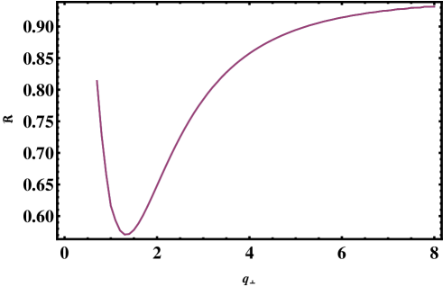
Figure 1: The double ration ${\cal R}$ as the function of $q_{\perp}$ for $\Delta_{\perp}=0.1\ GeV$.

III Observable

In Ref. Hatta:2016dxp , it has been proposed to probe the elliptic gluon GTMD by measuring diffractive dijet production in electron-nucleus collisions. Such process was first studied in Ref. Altinoluk:2015dpi . In the back-to-back kinematical limit where the individual jet transverse momentum $P_{\perp}$ is much larger than the nucleon recoiled momentum $\Delta_{\perp}$, a $\cos 2(\phi_{P_{\perp}}-\phi_{\Delta_{\perp}})$ angular modulation of the cross section of this process is sensitive to the elliptic gluon GTMD. Instead of the diffractive dijet production in eA collisions, we now consider transversely polarized virtual photon-nucleus quasi-elastic scattering $\gamma^{*}(q)+A(P)\rightarrow A(P^{\prime})+X$, which also offers us the opportunity to probe the elliptic gluon distribution via the angular correlation $\cos 2(\phi_{\epsilon_{T}^{\gamma^{*}}}-\phi_{\Delta_{\perp}})$ where $\epsilon_{T}^{\gamma^{*}}$ is the virtual photon transverse polarization vector.

In the dipole approach, the diffractive cross section for a transversely polarized virtual photon scattering off nucleus has been computed in Refs. Buchmuller:1998jv ; Kovchegov:1999kx and takes form,

$$\frac{d\sigma_{T}}{d^{2}\Delta_{\perp}} = \pi\int\frac{dz}{z(1-z)}\int d^{2}r_{\perp}|\Psi^{\gamma^{*}}_{T}(Q^{2},r_{\perp},z)|^{2}$$ (20)

$$\times\left\{\int\frac{d^{2}b_{\perp}}{(2\pi)^{2}}e^{-ib_{\perp}\cdot\Delta_{\perp}}\left[1-\left\langle\frac{1}{N_{c}}{\rm Tr}\left[U(b_{\perp}+\frac{r_{\perp}}{2})U^{\dagger}(b_{\perp}-\frac{r_{\perp}}{2})\right]\right\rangle\right]\right\}^{2}$$

where $\Psi^{\gamma^{*}}_{T}(Q^{2},r_{\perp},z)$ is the transversely polarized virtual photon wave function. The wave function squared can be expressed as,

$$|\Psi^{\gamma^{*}}_{T}\!(Q^{2},r_{\perp},z)|^{2}\!=2N_{c}\sum_{q}\!\frac{\alpha_{em}e_{q}^{2}}{\pi}z(1-z)\frac{(1-2z)^{2}(\epsilon_{T}^{\gamma^{*}}\!\!\cdot r_{\perp})^{2}+(\epsilon_{T}^{\gamma^{*}}\!\!\times r_{\perp})^{2}}{r_{\perp}^{2}}\epsilon_{f}^{2}\left[K_{1}(|r_{\perp}|e_{f})\right]^{2}$$ (21)

where $e_{f}^{2}=Q^{2}z(1-z)$ and $z$ is the longitudinal momentum fraction of virtual photon carried by quark. Here, quark mass is ignored. Inserting the MV model results, the azimuthal independent cross section is expressed as,

$$\frac{d\sigma_{T}}{d^{2}\Delta_{\perp}} = \pi\int\frac{dz}{z(1-z)}\int d^{2}r_{\perp}\Phi(Q^{2},r_{\perp}^{2},z)\left\{\int\frac{d^{2}b_{\perp}}{(2\pi)^{2}}e^{-ib_{\perp}\cdot\Delta_{\perp}}\left(1-e^{-\frac{r_{\perp}^{2}Q_{s}^{2}}{4}}\right)\right\}^{2}$$ (22)

while the azimuthal dependent cross section reads,

$$\frac{d\sigma_{T}}{d^{2}\Delta_{\perp}}|_{\cos 2\phi} = \frac{2(\epsilon_{T}^{\gamma^{*}}\cdot\Delta_{\perp})^{2}-\Delta_{\perp}^{2}}{24\Delta_{\perp}^{2}}\pi\int\frac{dz}{z(1-z)}\int d|r_{\perp}|\Phi^{\cal E}(Q^{2},r_{\perp}^{2},z)|r_{\perp}|^{5}$$ (23)

$$\times \int d|b_{\perp}|J_{2}(|\Delta_{\perp}||b_{\perp}|)|b_{\perp}|^{3}\frac{\partial^{2}Q_{s}^{2}(b_{\perp}^{2})}{\partial^{2}b_{\perp}^{2}}e^{-\frac{r_{\perp}^{2}Q_{s}^{2}(b_{\perp}^{2})}{4}}\int\frac{d^{2}b_{\perp}^{\prime}}{(2\pi)^{2}}\left(1-e^{-\frac{r_{\perp}^{2}Q_{s}^{2}(b_{\perp}^{\prime 2})}{4}}\right)$$

with the scalar part of the wave function being given by,

$$\Phi(Q^{2},r_{\perp}^{2},z) = 2N_{c}\sum_{q}\frac{\alpha_{em}e_{q}^{2}}{\pi}z(1-z)[z^{2}+(1-z)^{2}]\epsilon_{f}^{2}\left[K_{1}(|r_{\perp}|e_{f})\right]^{2}$$ (24)

$$\Phi^{\cal E}(Q^{2},r_{\perp}^{2},z) = 2N_{c}\sum_{q}\frac{\alpha_{em}e_{q}^{2}}{\pi}z(1-z)[2z^{2}-2z]\epsilon_{f}^{2}\left[K_{1}(|r_{\perp}|e_{f})\right]^{2}$$ (25)

If the virtual photon is induced by a lepton, only the $V_{4}$ component Meng:1991da ; Zhou:2008fb of the corresponding leptonic tensor contributes to the azimuthal dependent cross section. To be precise, the contribution from this component yields a $\cos 2\phi_{e-A}$ azimuthal modulation where $\phi_{e-A}$ is the angle between the hadron/nucleus plane and the lepton plane. One notices that the azimuthal asymmetry in this process offers us a direct access to the second derivative of the saturation scale with respect to $b_{\perp}^{2}$. As such, the elliptic gluon GTMD can be easily determined through measuring this observable.

IV Summary

We derived the elliptic gluon GTMD inside a large nucleus using the MV model. Our result can be used as the initial condition when implementing small $x$ evolution. We further proposed to probe the elliptic gluon GTMD through the angular correlation in quasi-elastic virtual photon scattering off a nucleus. This measurement can, in principle, be carried out at the future EIC. Since a such study will deepen our understanding how the gluon tomography is induced by small $x$ dynamics, it might be worthwhile to pursue a comprehensive numerical analysis of this observable for the typical EIC accessible kinematical region in a future publication.

Acknowledgments: I would like to thank D. Mueller for bringing my attention to the small $x$ gluon helicity flip GPDs, and Y. J. Zhou for her help with making the plot. This work has been supported by the National Science Foundations of China under Grant No. 11160005131608, and by the Thousand Talents Plan for Young Professionals.

References

• (1) X. d. Ji, Phys. Rev. Lett.  91, 062001 (2003) doi:10.1103/PhysRevLett.91.062001 [hep-ph/0304037].
• (2) A. V. Belitsky, X. d. Ji and F. Yuan, Phys. Rev. D 69, 074014 (2004) doi:10.1103/PhysRevD.69.074014 [hep-ph/0307383].
• (3) C. Lorce and B. Pasquini, Phys. Rev. D 84, 014015 (2011) doi:10.1103/PhysRevD.84.014015 [arXiv:1106.0139 [hep-ph]].
• (4) C. Lorce, B. Pasquini, X. Xiong and F. Yuan, Phys. Rev. D 85, 114006 (2012) doi:10.1103/PhysRevD.85.114006 [arXiv:1111.4827 [hep-ph]].
• (5) S. Meissner, A. Metz and M. Schlegel, JHEP 0908, 056 (2009) doi:10.1088/1126-6708/2009/08/056 [arXiv:0906.5323 [hep-ph]].
• (6) A. Mukherjee, S. Nair and V. K. Ojha, Phys. Rev. D 90, no. 1, 014024 (2014) doi:10.1103/PhysRevD.90.014024 [arXiv:1403.6233 [hep-ph]].
• (7) A. Courtoy, G. R. Goldstein, J. O. Gonzalez Hernandez, S. Liuti and A. Rajan, Phys. Lett. B 731, 141 (2014) doi:10.1016/j.physletb.2014.02.017 [arXiv:1310.5157 [hep-ph]].
• (8) K. Kanazawa, C. Lorce, A. Metz, B. Pasquini and M. Schlegel, Phys. Rev. D 90, no. 1, 014028 (2014) doi:10.1103/PhysRevD.90.014028 [arXiv:1403.5226 [hep-ph]].
• (9) T. Liu and B. Q. Ma, Phys. Rev. D 91, 034019 (2015) doi:10.1103/PhysRevD.91.034019 [arXiv:1501.07690 [hep-ph]].
• (10) A. Mukherjee, S. Nair and V. K. Ojha, Phys. Rev. D 91, no. 5, 054018 (2015) doi:10.1103/PhysRevD.91.054018 [arXiv:1501.03728 [hep-ph]].
• (11) D. Chakrabarti, T. Maji, C. Mondal and A. Mukherjee, Eur. Phys. J. C 76, no. 7, 409 (2016) doi:10.1140/epjc/s10052-016-4258-7 [arXiv:1601.03217 [hep-ph]].
• (12) C. Lorce and B. Pasquini, JHEP 1309, 138 (2013) doi:10.1007/JHEP09(2013)138 [arXiv:1307.4497 [hep-ph]].
• (13) C. Lorce and B. Pasquini, Phys. Rev. D 93, no. 3, 034040 (2016) doi:10.1103/PhysRevD.93.034040 [arXiv:1512.06744 [hep-ph]].
• (14) M. G. Echevarria, A. Idilbi, K. Kanazawa, C. Lorce A. Metz, B. Pasquini and M. Schlegel, Phys. Lett. B 759, 336 (2016) doi:10.1016/j.physletb.2016.05.086 [arXiv:1602.06953 [hep-ph]].
• (15) Y. Hatta, Phys. Lett. B 708, 186 (2012) doi:10.1016/j.physletb.2012.01.024 [arXiv:1111.3547 [hep-ph]].
• (16) S. J. Brodsky, L. Frankfurt, J. F. Gunion, A. H. Mueller and M. Strikman, Phys. Rev. D 50, 3134 (1994) doi:10.1103/PhysRevD.50.3134 [hep-ph/9402283].
• (17) W. Buchmuller, T. Gehrmann and A. Hebecker, Nucl. Phys. B 537, 477 (1999) doi:10.1016/S0550-3213(98)00682-8 [hep-ph/9808454].
• (18) Y. V. Kovchegov and L. D. McLerran, Phys. Rev. D 60, 054025 (1999) Erratum: [Phys. Rev. D 62, 019901 (2000)] doi:10.1103/PhysRevD.62.019901, 10.1103/PhysRevD.60.054025 [hep-ph/9903246].
• (19) A. D. Martin, M. G. Ryskin and T. Teubner, Phys. Rev. D 62, 014022 (2000) doi:10.1103/PhysRevD.62.014022 [hep-ph/9912551].
• (20) H. Kowalski and D. Teaney, Phys. Rev. D 68, 114005 (2003) doi:10.1103/PhysRevD.68.114005 [hep-ph/0304189].
• (21) C. Marquet, R. B. Peschanski and G. Soyez, Phys. Rev. D 76, 034011 (2007) doi:10.1103/PhysRevD.76.034011 [hep-ph/0702171 [HEP-PH]].
• (22) T. Lappi and H. Mantysaari, Phys. Rev. C 83, 065202 (2011) doi:10.1103/PhysRevC.83.065202 [arXiv:1011.1988 [hep-ph]].
• (23) A. H. Rezaeian, M. Siddikov, M. Van de Klundert and R. Venugopalan, Phys. Rev. D 87, no. 3, 034002 (2013) doi:10.1103/PhysRevD.87.034002 [arXiv:1212.2974 [hep-ph]].
• (24) F. Dominguez, C. Marquet, B. W. Xiao and F. Yuan, Phys. Rev. D 83, 105005 (2011) doi:10.1103/PhysRevD.83.105005 [arXiv:1101.0715 [hep-ph]].
• (25) J. Zhou, JHEP 1606, 151 (2016) doi:10.1007/JHEP06(2016)151 [arXiv:1603.07426 [hep-ph]].
• (26) Y. Hatta, B. W. Xiao and F. Yuan, Phys. Rev. Lett.  116, no. 20, 202301 (2016) doi:10.1103/PhysRevLett.116.202301 [arXiv:1601.01585 [hep-ph]].
• (27) P. Hoodbhoy and X. D. Ji, Phys. Rev. D 58, 054006 (1998) doi:10.1103/PhysRevD.58.054006 [hep-ph/9801369].
• (28) A. V. Belitsky and D. Mueller, Phys. Lett. B 486, 369 (2000) doi:10.1016/S0370-2693(00)00773-5 [hep-ph/0005028].
• (29) L. N. Lipatov, Sov. Phys. JETP 63, 904 (1986) [Zh. Eksp. Teor. Fiz.  90, 1536 (1986)].
• (30) H. Navelet and S. Wallon, Nucl. Phys. B 522, 237 (1998) doi:10.1016/S0550-3213(98)00146-1 [hep-ph/9705296].
• (31) H. Navelet and R. B. Peschanski, Nucl. Phys. B 507, 353 (1997) doi:10.1016/S0550-3213(97)00568-3 [hep-ph/9703238].
• (32) K. J. Golec-Biernat and A. M. Stasto, Nucl. Phys. B 668, 345 (2003) doi:10.1016/j.nuclphysb.2003.07.011 [hep-ph/0306279].
• (33) C. Marquet and G. Soyez, Nucl. Phys. A 760, 208 (2005) doi:10.1016/j.nuclphysa.2005.05.198 [hep-ph/0504080].
• (34) B. Z. Kopeliovich, H. J. Pirner, A. H. Rezaeian and I. Schmidt, Phys. Rev. D 77, 034011 (2008) doi:10.1103/PhysRevD.77.034011 [arXiv:0711.3010 [hep-ph]].
• (35) Y. Hagiwara, Y. Hatta and T. Ueda, arXiv:1609.05773 [hep-ph].
• (36) L. D. McLerran and R. Venugopalan, Phys. Rev. D 49, 3352 (1994) doi:10.1103/PhysRevD.49.3352 [hep-ph/9311205]; Phys. Rev. D 49, 2233 (1994) doi:10.1103/PhysRevD.49.2233 [hep-ph/9309289].
• (37) Y. V. Kovchegov, Phys. Rev.  D54, 5463-5469 (1996). [hep-ph/9605446].
• (38) J. Jalilian-Marian, A. Kovner, L. D. McLerran, H. Weigert, Phys. Rev.  D55, 5414-5428 (1997). [hep-ph/9606337].
• (39) A. Metz and J. Zhou, Phys. Rev. D 84, 051503 (2011) doi:10.1103/PhysRevD.84.051503 [arXiv:1105.1991 [hep-ph]].
• (40) A. Dumitru, T. Lappi and V. Skokov, Phys. Rev. Lett.  115, no. 25, 252301 (2015) doi:10.1103/PhysRevLett.115.252301 [arXiv:1508.04438 [hep-ph]].
• (41) J. Zhou, Phys. Rev. D 89, no. 7, 074050 (2014) doi:10.1103/PhysRevD.89.074050 [arXiv:1308.5912 [hep-ph]].
• (42) Y. V. Kovchegov and M. D. Sievert, Phys. Rev. D 86, 034028 (2012) Erratum: [Phys. Rev. D 86, 079906 (2012)] doi:10.1103/PhysRevD.86.034028, 10.1103/PhysRevD.86.079906 [arXiv:1201.5890 [hep-ph]].
• (43) L. Szymanowski and J. Zhou, Phys. Lett. B 760, 249 (2016) doi:10.1016/j.physletb.2016.06.055 [arXiv:1604.03207 [hep-ph]].
• (44) D. Boer, M. G. Echevarria, P. Mulders and J. Zhou, Phys. Rev. Lett.  116, no. 12, 122001 (2016) doi:10.1103/PhysRevLett.116.122001 [arXiv:1511.03485 [hep-ph]].
• (45) D. Boer, S. Cotogno, T. van Daal, P. J. Mulders, A. Signori and Y. J. Zhou, JHEP 1610, 013 (2016) doi:10.1007/JHEP10(2016)013 [arXiv:1607.01654 [hep-ph]].
• (46) P. J. Mulders and J. Rodrigues, Phys. Rev. D 63, 094021 (2001) doi:10.1103/PhysRevD.63.094021 [hep-ph/0009343].
• (47) D. Boer, P. J. Mulders, C. Pisano and J. Zhou, JHEP 1608, 001 (2016) doi:10.1007/JHEP08(2016)001 [arXiv:1605.07934 [hep-ph]].
• (48) J. Bartels, Nucl. Phys. B 175, 365 (1980). doi:10.1016/0550-3213(80)90019-X. J. Kwiecinski and M. Praszalowicz, Phys. Lett.  94B, 413 (1980). doi:10.1016/0370-2693(80)90909-0
• (49) T. Altinoluk, N. Armesto, G. Beuf and A. H. Rezaeian, Phys. Lett. B 758, 373 (2016) doi:10.1016/j.physletb.2016.05.032 [arXiv:1511.07452 [hep-ph]].
• (50) R. b. Meng, F. I. Olness and D. E. Soper, Nucl. Phys. B 371, 79 (1992). doi:10.1016/0550-3213(92)90230-9
• (51) J. Zhou, F. Yuan and Z. T. Liang, Phys. Rev. D 78, 114008 (2008) doi:10.1103/PhysRevD.78.114008 [arXiv:0808.3629 [hep-ph]].