NonSTOP: A NonSTationary Online Prediction Method for Time Series

Abstract

We present online prediction methods for time series that let us explicitly handle nonstationary artifacts (e.g. trend and seasonality) present in most real time series. Specifically, we show that applying appropriate transformations to such time series before prediction can lead to improved theoretical and empirical prediction performance. Moreover, since these transformations are usually unknown, we employ the learning with experts setting to develop a fully online method (NonSTOP-NonSTationary Online Prediction) for predicting nonstationary time series. This framework allows for seasonality and/or other trends in univariate time series and cointegration in multivariate time series. Our algorithms and regret analysis subsume recent related work while significantly expanding the applicability of such methods. For all the methods, we provide sub-linear regret bounds using relaxed assumptions. The theoretical guarantees do not fully capture the benefits of the transformations, thus we provide a data-dependent analysis of the follow-the-leader algorithm that provides insight into the success of using such transformations. We support all of our results with experiments on simulated and real data.

1 Introduction

Time series modeling and forecasting is fundamentally important in many domains including econometrics and resource consumption forecasting [Hamilton, 1994]. Analyzing and forecasting stationary time series models such as AutoRegressive Moving Average (ARMA) models Box et al. [2008], Brockwell and Davis [2009], Hamilton [1994] has been well-studied. However, the inherently complex structure of real world data is more appropriately modeled by nonstationary time series. Time series that exhibit such nonstationary structure include seasonal time series such as influenza rates [ILI, ], and time series exhibiting trends such as housing indexes and stock market prices [SP, ]. Such data are ubiquitous and will only continue to grow as technology develops, especially with the Internet of Things where devices will generate large quantities of nonstationary time series data. Thus, efficient estimation and prediction with such models will become much more relevant.

In the setting of streaming or high-frequency time series, one would ideally like to have methods that update the model, predict sequentially, and do not rely on any restricting assumptions on the noise sequence or the loss function. This brings attention to the paradigm of online learning [Cesa-Bianchi and Lugosi, 2006]. In that vein, Anava et al. [2013] recently presented online gradient descent (OGD) and online Newton step (ONS) methods (ARMA-OGD and ARMA-ONS) for ARMA prediction that do not make the Gaussianity assumption. Using a truncated auto-regressive (AR) representation of an ARMA process, the authors provide online ARMA prediction algorithms with sublinear regret, where the regret is with respect to the best conditionally expected one-step ARMA prediction loss in hindsight. While no assumption is made about the stationarity of the generating ARMA process, the empirical performance of ARMA-OGD suffers in the presence of seasonality and/or trends Liu et al. [2016].

To handle a deterministic or stochastic trend, Liu et al. [2016] recently presented ARIMA-OGD, a straigtforward extension of ARMA-OGD using AutoRegressive Integrated Moving Average (ARIMA) models. However, the trend transform and its parameters (e.g. order of integration) are assumed to be known, which is unrealistic in online settings as one typically needs adequate data to test for such nonstationarities. Moreover, these methods don’t account for seasonality and do not carry over to the multivariate domain. These shortcomings of existing work necessitate the development of broader methods that take into account different types of nonstationarities with extensions to multivariate time series.

1.1 Contributions

We provide general methods for time series prediction using OGD [Zinkevich, 2003] that account for possible nonstationarities in the data. This leads to explicit transformations of the data before prediction when the form of these nonstationarities are known. In the univariate case, our approach subsumes existing work while expanding the applicability of such online methods to more realistic time series settings. For the multivariate case, we propose a novel algorithm for prediction of nonstationary vector time series generated by Error Corrected Vector AutoRegressive Moving Average (EC-VARMA) processes to deal with the phenomenon of cointegration [Tsay, 2013, Lütkepohl, 2005]. Estimating EC-VARMA models are non-trivial in general; this typically requires a two-stage process where the cointegrating rank is estimated before the parameters are estimated. The algorithm we propose simultaneously estimates both the cointegrating rank and the VARMA (Vector AutoRegressive Moving Average) matrix parameters.

However, the form of the nonstationary transformations are usually unknown. These transforms are typically determined by statistical tests on a fixed dataset with sample size requirements. In the online setting, this is unrealistic, thus we unify the above methods into a meta-algorithm called NonSTOP to learn the correct transformation in an online fashion. NonSTOP utilizes the weighted majority method Cesa-Bianchi and Lugosi [2006] wherein each expert corresponds to different parameter settings of the nonstationary transformation (e.g. trend only, trend and seasonality, no trend/seasonality, etc). NonSTOP quickly hones in on the correct transformation, and also allows for flexibility in adapting to changes in the data.

Our regret analysis, which provides sublinear regret guarantees for all methods, only requires invertibility of the moving average polynomial while the assumptions in Anava et al. [2013] and Liu et al. [2016] are less natural. Moreover, we don’t require an upper bound on the data as nonstationary data can be unbounded.

To emphasize the effect of the these nonstationary transformations, we prove a data dependent regret guarantee for FTL (for least squares loss) that gives insights into why adjusting for nonstationarities can give faster convergence.

All proofs can be found in the supplement.

1.2 Related Work

The application of online learning to time series modeling has begun to receive more attention in the past couple of years. Anava et al. [2013] developed online gradient and online second order methods for ARMA prediction. Liu et al. [2016] present a trend extension to Anava et al. [2013] that requires knowledge of the parameters of the trend transformation, which is unrealistic in the online setting. Other extensions include application to missing data Anava et al. [2015] and heteroscedastic processes Anava and Mannor [2016]. However, these algorithms suffer in the presence of seasonliaty and are not applicable to multivariate time series. In contrast, we provide a unified general framework capable of efficiently handling many common types of nonstationarities found in real data.

Few works have tackled the problem of forecasting nonstationary time series in an online fashion. Kuznetsov and Mohri [2016] developed generalization bounds for nonstationary time series prediction by using online-to-batch conversion techniques on the sequences of hypothesis output by a online algorithm for time series prediction. However, the work develops guarantees for the batch setting as opposed to the online (possibly adversarial) setting and the method presented is in general computationally intensive. Recently, Hazan et al. [2017] presented an online prediction method for a linear dynamical system and also provided optimal regret bounds. Even though general state space models allow for nonstationary components, these were not explored in the work. While ARMA models do have a linear dynamical system representation, their natural form is more parsimonious for explicitly modeling different kinds of nonstationarity.

2 Preliminaries: Time Series Modeling

In this section, we provide a brief summary of SARIMA (Seasonal ARIMA) and EC-VARMA processes. For more comprehensive background, see Box et al. [2008], Tsay [2013]. For an introduction to online convex optimzation and online gradient descent, please see [Shalev-Shwartz, 2011, Zinkevich, 2003, Hazan et al., 2007]. We introduce standard notation for time series in Table 1. Note that the differencing notation $\Delta$ can be compounded: $\Delta^{2}x_{t}=\Delta(x_{t}-x_{t-1})=x_{t}-2x_{t-1}+x_{t-2}$.

Table 1: Notation

$B$	$Bx_{t}=x_{t-1}$
$\Delta$	$\Delta x_{t}=x_{t}-x_{t-1}$
$\Delta_{s}$	$\Delta_{s}x_{t}=x_{t}-x_{t-s}$
$d$	Differencing order
$s$	Seasonal period
$\tilde{D}$	Seasonal differencing order

2.1 SARIMA

Time series exhibiting seasonal patterns can be modeled by Seasonal AutoRegressive Integrated Moving Average (SARIMA) Processes. Let $x_{t},\varepsilon_{t}\in\mathbb{R}$ denote the time series and innovations (random variables). SARIMA$(p,d,q)\times(P,\tilde{D},Q)_{s}$ processes are described by the following:

$$\phi(B)\Phi(B^{s})\Delta^{d}\Delta^{\tilde{D}}_{s}x_{t}=\theta(B)\Theta(B^{s})\varepsilon_{t}$$ (1)

where $\phi(B)=1-\sum_{{i}=1}^{p}\phi_{i}B^{i},\theta(B)=1+\sum_{{i}=1}^{q}\theta_{i}B^{i}$, $\Phi(B^{s})=1-\sum_{{i}=1}^{P}\Phi_{i}B^{is},\Theta(B^{s})=1+\sum_{{i}=1}^{Q}\Theta_{i}B^{is}$ and $\phi,\Phi,\theta,\Theta\in\mathbb{R}$. Note that $\tilde{D}=0$ implies a ARIMA($p,d,q$) process, and $\tilde{D}=d=0$ implies a ARMA($p,q$) process.

SARIMA processes explicitly model trend and seasonal nonstationarities by assuming that the differenced process $\Delta^{d}\Delta^{\tilde{D}}_{s}x_{t}$ is an ARMA process with AR lag polynomial $\phi(B)\Phi(B^{s})$ and MA lag polynomial $\theta(B)\Theta(B^{s})$. We denote the order of the underlying AR and MA lag polynomials as $l_{a}$ and $l_{m}$, respectively. For SARIMA$(p,d,q)\times(P,\tilde{D},Q)_{s}$ processes, Eq. (1) gives us that $l_{a}=p+Ps$ and $l_{m}=q+Qs$.

If the MA lag polynomial has all of its roots outside of the complex unit circle, then the SARIMA process is defined as invertible. Invertibility is equivalent to saying that the companion matrix (see Supplement) has eigenvalues less than 1 in magnitude. If this is the case, then the underlying ARMA process $\Delta^{d}\Delta^{\tilde{D}}_{s}x_{t}$ can be written as an AR$(\infty)$ process and can be approximated by a finite truncated AR process.

2.2 EC-VARMA

In many cases, a collection of time series may follow a common trend. This phenomenon, known as cointegration, is ubiquitous in economic times series [Tsay, 2013]. Let $\mathbf{x}_{t},\bm{\varepsilon}_{t}\in\mathbb{R}^{k},\bm{\Phi}_{i}\in\mathbb{R}^{k\times k},\bm{\Theta}_{i}\in\mathbb{R}^{k\times k}$. First, a VARMA$(p,q)$ process is described by:

$$\mathbf{x}_{t}=\sum_{{i}=1}^{p}\bm{\Phi}_{i}\mathbf{x}_{t-i}+\sum_{{i}=1}^{q}\bm{\Theta}_{i}\bm{\varepsilon}_{t-i}+\bm{\varepsilon}_{t}$$ (2)

which is equivalent to writing $\bm{\Phi}(B)\mathbf{x}_{t}=\bm{\Theta}(B)\bm{\varepsilon}_{t}$ where $\bm{\Phi}(B)=I-\sum_{{i}=1}^{p}\bm{\Phi}_{i}B^{i},\bm{\Theta}(B)=I+\sum_{{i}=1}^{q}\bm{\Theta}_{i}B^{i}$. Formally, $\mathbf{x}_{t}$ is cointegrated if $\Delta\mathbf{x}_{t}$ is stationary and there exists a vector $\mu\in\mathbb{R}^{k}$ such that $\mu^{\intercal}\mathbf{x}_{t}$ is a stationary process. If $\mathbf{x}_{t}$ is cointegrated, then we can rewrite the original VARMA representation of $\mathbf{x}_{t}$ as

$$\Delta\mathbf{x}_{t}=\Pi\mathbf{x}_{t-1}+\sum_{{i}=1}^{p-1}\Gamma_{i}\Delta\mathbf{x}_{t-i}+\sum_{{i}=1}^{q}\bm{\Theta}_{i}\bm{\varepsilon}_{t-i}+\bm{\varepsilon}_{t}$$ (3)

where $\Pi=\bm{\Phi}(1)$, denoted the cointegrating matrix, is low rank (cointegrating rank), and $\Gamma_{j}=-(\bm{\Phi}_{j+1}+\ldots+\bm{\Phi}_{p})$ for $j=1,\ldots p-1$. Eq. (3) is known as an Error-Corrected VARMA (EC-VARMA) model. Given that an such a process starts at some fixed time $t=0$ with fixed initial values, we can write Eq. (3) in a pure EC-VAR form Lütkepohl [2006]:

$$\Delta\mathbf{x}_{t}=\Pi^{*}\mathbf{x}_{t-1}+\sum_{{i}=1}^{t-1}\Gamma_{i}^{*}\Delta\mathbf{x}_{t-i}+\bm{\varepsilon}_{t},\ \ \ t\in\mathbb{N}$$ (4)

This allows us to approximate an EC-VARMA process with an EC-VAR model.

3 Univariate Methods

In this section, we present algorithms for online univariate time series prediction which subsumes recent works such as ARMA-OGD as presented in Anava et al. [2013] and its the extension to trend nonstationarities ARIMA-OGD as presented in Liu et al. [2016].

We show that time series with certain characteristics (such as a trend and/or seasonality) can be transformed before prediction to give better theoretical and empirical results. To achieve this goal, we present a unified template for Time Series Prediction using OGD, denoted TSP-OGD, that allows for prediction of transformed time series. The choice of the transformation, dependent on the underlying data generation process (DGP), can lead to improved regret guarantees, partially explaining why these transformations lead to better empirical performance.

This framework includes some commonly used transformations [Box et al., 2008]. Table 2 shows the explicit form of such transformations. In practice, the order of differencing is usually determined by statistical tests (e.g. Elliot et al. [1996]) on a given dataset, which is not realistic when considering the online setting.

3.1 TSP-OGD

We assume the following for the remainder of this section:

• $x_{t}$ is generated by a DGP such that there exists a transformation $\tau(x_{t})$ which results in an invertible ARMA process. Moreover, there corresponds an inverse transformation $\zeta$ that satisfies $\zeta(\tau(x_{t}))=x_{t}$. Examples of such processes are ARMA, ARIMA, and SARIMA processes.

• The noise sequence $\varepsilon_{t}$ of the process is independent. Also, it satisfies that $\mathbb{E}[|\varepsilon_{t}|]<M_{\textrm{max}}<\infty$.

• $\ell_{t}:\mathbb{R}^{2}\rightarrow\mathbb{R}$ is a convex loss function with Lipschitz constant $L>0$.

• We assume the companion matrix $\mathbf{F}$ (as defined in the Supplement) of the MA lag polynomial is diagonalizable, i.e. $\mathbf{F}=\mathbf{T}\Lambda\mathbf{T}^{-1}$ where $\Lambda$ is a diagonal matrix of eigenvalues. Denote $\lambda_{\max}$ as the magnitude of the largest eigenvalue ($\lambda_{\max}<1$ by definition of invertibility), and $\kappa\in\mathbb{R}$ such that $\left(\sigma_{\max}(\mathbf{T})/\sigma_{\min}(\mathbf{T})\right)\leq\kappa$.

Assumption U1 includes a large class of models including ARMA/ARIMA/SARIMA models. It is well-known that the class of ARMA models is equivalent to linear state space models, thus that class of models is included in U1. U2 and U3 are standard assumptions in the time series literature. Lastly, U4 is a relaxation of the less natural assumptions present in previous works Anava et al. [2013], Liu et al. [2016]. Our assumption only requires the invertibility of the MA process, which guarantees that the process can be well-approximated by a finite AR process (which is the heart of our framework). Note that we don’t make the assumption that the data is bounded (as in previous works), as data generated by a nonstationary process can be unbounded (e.g. random walks).

Algorithm 1 TSP-OGD Framework

0:  DGP parameters $l_{a},l_{m}$. Horizon $T$. Learning rate $\eta$. Data: $\{x_{t}\}$. Transformation $\tau$. Inverse Transformation $\zeta$.

1:  Set $M=\log_{\lambda_{\max}}\left(\left(2\kappa TLM_{\max}\sqrt{l_{m}}\right)^{-1}\right)+l_{a}$

2:  Transform $x_{t}$ to get $\tau(x_{t})$.

3:  Choose $\bm{\gamma}^{(1)}\in\mathcal{E}$ arbitrarily.

4:  for $t=1$ to $T$ do

5:     $\tau\left(\tilde{x}_{t}\right)=\sum_{{i}=1}^{M}\bm{\gamma}^{(t)}_{i}\tau\left(x_{t-i}\right)$

6:     Predict $\tilde{x}_{t}=\zeta(\tau(\tilde{x}_{t}))$

7:     Observe $x_{t}$ and receive loss $\ell_{t}^{M}\left(\bm{\gamma}^{(t)}\right)$

8:     Set $\bm{\gamma}^{(t+1)}=\Pi_{\mathcal{E}}\left(\bm{\gamma}^{(t)}-\eta\nabla\ell_{t}^{M}\left(\bm{\gamma}^{(t)}\right)\right)$

9:  end for

Table 2: DGPs and their Transformations

DGP	$\tau(x_{t})$	$\zeta(y_{t})$
ARMA	$x_{t}$	$y_{t}$
ARIMA	$\Delta^{d}x_{t}$	$y_{t}+\sum_{i=0}^{d-1}\Delta^{i}x_{t-1}$
SARIMA	$\Delta^{d}\Delta^{\tilde{D}}_{s}x_{t}$	$\begin{array}[]{lcl}y_{t}&+&\sum_{i=0}^{d-1}\Delta^{i}\Delta_{s}^{\tilde{D}}x_{t-1}\\ &+&\sum_{i=0}^{{\tilde{D}}-1}\Delta_{s}^{i}x_{t-s}\end{array}$

In Algorithm 1, the model parameters of the stochastic process are fixed by an adversary. At time $t$, $\varepsilon_{t}$ and $x_{t}$ are generated by the DGP. Before $x_{t}$ is revealed to us, the learner makes a prediction $\tilde{x}_{t}$ (see line 6 of Algorithm 1) which incurs a prediction loss of $\ell_{t}(x_{t},\tilde{x}_{t})$. In more detail, this prediction is preceded by a transform $\tau$ (See Table 2) that may require data points from previous rounds (we suppress that dependence in the notation for convenience). The prediction $\tau(\tilde{x}_{t}):=\sum_{{i}=1}^{M}\gamma_{i}\tau\left(x_{t-i}\right)$ is computed using an AR model of order $M$ to approximate the underlying invertible ARMA process. Then it is inverted with $\zeta$ and incurs a loss

$$\ell_{t}^{M}(\bm{\gamma}) :=\ell_{t}\left(x_{t},\zeta\left(\sum_{{i}=1}^{M}\gamma_{i}\tau\left(x_{t-i}\right)\right)\right)$$ (5)

where $\bm{\gamma}$ is the vector of parameters of the approximating AR model. The prediction performance is evaluated using an “extended” notion of regret that looks at the prediction loss of the best process in hindsight. Precisely, let $\bm{\alpha},\bm{\beta}$ denote the set of AR and MA parameters, respectively, of the underlying ARMA process $\tau(x_{t})$. Define

$$f_{t}(\bm{\alpha},\bm{\beta})=\ell_{t}\left(x_{t},\zeta\left(\mathbb{E}\left[\tau(x_{t})|\{\tau\left(x_{t}\right)\}_{t=1}^{t-1};\bm{\alpha},\bm{\beta}\right]\right)\right)$$ (6)

Note that $f_{t}$ depends on the transformations $\tau,\zeta$ in U1. The extended regret is defined as comparing the accumulated loss in Eq. (5) to the loss of the best process in hindsight:

$$\text{Regret}=\sum_{{t}=1}^{T}\ell_{t}^{M}(\bm{\gamma}^{(t)})-\min_{\bm{\alpha},\bm{\beta}\in\mathcal{K}}\sum_{{t}=1}^{T}\mathbb{E}[f_{t}(\bm{\alpha},\bm{\beta})]$$ (7)

where $\mathcal{K}$ is the set of invertible ARMA processes.

Furthermore, let $\mathcal{E}\subseteq\mathbb{R}^{M}$ be a convex set of approximating AR models, i.e. $\bm{\gamma}\in\mathcal{E}$. $\mathcal{E}$ should be chosen to be large enough to include a valid approximation to the DGP described in U1. However, since the DGP is unknown in practice, one usually chooses a simple constraint set such as $\mathcal{E}=\{\bm{\gamma}:\|\bm{\gamma}\|_{\infty}\leq 1\}$. Let $D=\sup_{\bm{\gamma}_{1},\bm{\gamma}_{2}\in\mathcal{E}}\|\bm{\gamma}_{1}-\bm{\gamma}_{2}\|_{2}$, and $\|\nabla_{\bm{\gamma}}\ell_{t}^{M}(\bm{\gamma})\|_{2}\leq G(t)$ for some monotonically increasing $G(t)$. This assumption allows the time series to be potentially unbounded. Let $\Pi_{\mathcal{E}}$ denote the projection operator onto the set $\mathcal{E}$.

We present a general regret bound for Algorithm 1:

Theorem 3.1.

Let $\eta=\frac{D}{G(T)\sqrt{T}}$. Then for any data sequence $\{x_{t}\}_{t=1}^{T}$ that satisfies assumptions U1-U4, Algorithm 1 generates a sequence $\{\bm{\gamma}^{(t)}\}$ in which

$$\text{Regret}=O\left(DG(T)\sqrt{T}\right)$$

Remark 1: Note that plugging in the ARMA transformation and ARIMA transformation in Table 2 to Algorithm 1 recovers ARMA-OGD as presented in Anava et al. [2013] and ARIMA-OGD as presented in Liu et al. [2016], respectively. Plugging in the SARIMA transformation results in a novel variation which we denote as SARIMA-OGD.

For the following remarks, assume that $\ell_{t}$ is squared loss, the DGP is a SARIMA process, and $|x_{t}|<C(t)=O\left(\log t\right)$ (note that the $\log$ transformation is commonly employed as a variance stabilizer in many time series domains).

Remark 2: Table 3 shows the regret bounds obtained by using different transformations/algorithms. The differencing transforms remove any growth trends in the data; as a consequence the transformed time series is bounded by a constant. In our case, this implies $|\Delta^{d}x_{t}|,|\Delta^{d}\Delta^{\tilde{D}}_{s}x_{t}|<C_{\Delta}$ (a constant), which leads to an improvement over the regret bound obtained from ARMA-OGD. This improvement can be seen in the empirical results section of Liu et al. [2016].

Remark 3: When the DGP is assumed to be SARIMA, we require that $l_{a}=p+Ps,l_{m}=q+Qs$ as mentioned in Section 2, i.e. $l_{a},l_{m}$ both need to essentially be a multiplicative factor larger than $s$. This affects the length of the required AR approximation $M$ as described in line 1 of Algorithm 1.

Table 3: Regret Bounds for Different Transformations

Algorithm	$\tau(x_{t})$	Regret Bound
ARMA-OGD	$x_{t}$	$O\left(M^{2}\log^{2}(T)\sqrt{T}\right)$
ARIMA-OGD	$\Delta^{d}x_{t}$	$O\left(M^{2}\sqrt{T}\right)$
SARIMA-OGD	$\Delta^{d}\Delta^{\tilde{D}}_{s}x_{t}$	$O\left(M^{2}\sqrt{T}\right)$

3.2 Data Transformation Dependent Regret

The transformations discussed in the previous sections essentially diminish serial correlation in the data due to any existing nonstationarities. However, our regret bounds (shown in Table 3) do not accurately reflect this. We conjecture that these bounds are missing data-dependent terms that capture correlations in nonstationary time series. To give a flavor of what a satisfactory data dependent regret bound might look like, we analyze the regret for the FTL algorithm for the case of least squares loss $\left(\ell_{t}(\bm{\gamma})=\frac{1}{2}(x_{t}-\bm{\gamma}^{\intercal}\bm{\psi}_{t})^{2}\right)$ and show that these bounds depend on a data dependent term. We look at the standard notion of regret and hence the result in this section is much more general than time series prediction and is also relevant to general regression problems.

The FTL algorithm follows a simple update [Shalev-Shwartz, 2011] $\left(\bm{\gamma}_{t+1}\in\operatornamewithlimits{argmin}_{\bm{\gamma}}\sum_{{i}=1}^{t}\ell_{t}(\bm{\gamma})\right)$. It is easy to see that the FTL algorithm for least squares loss is just recursive least squares (RLS). Using the relevant RLS update equations Ljung [1998], Lai and Wei [1982], we obtain the following:

Theorem 3.2.

Let $\ell_{t}(\bm{\gamma})$ be the squared loss with Lipschitz constant $L>0$. Then FTL generates a sequence $\{\bm{\gamma}_{t}\}$ in which

$$\sum_{{t}=1}^{T}\ell_{t}\left(\bm{\gamma}_{t}\right)-\min_{\bm{\gamma}}\sum_{{t}=1}^{T}\ell_{t}\left(\bm{\gamma}\right)=O\left(\sum_{{t}=1}^{T}\frac{1}{t\lambda_{\min}(t)}\right)$$

where $\lambda_{\min}(t):=\lambda_{\min}\left(\frac{1}{t}\sum_{{i}=1}^{t}\bm{\psi}_{i}\bm{\psi}_{i}^{\intercal}\right)$.

At the heart of our framework in Algorithm 1, we are approximating an ARMA process with an AR model. In order to apply Theorem 3.2 to our time series prediction setting for DGPs as described in assumption U1, assume for now that we use FTL and least squares loss to predict the underlying ARMA process $\tau(x_{t})$ with an AR model $\bm{\gamma}^{\intercal}\tau(\bm{\xi}_{t})$, where $\bm{\xi}_{t}=\begin{bmatrix}x_{t-1}&\ldots&x_{t-M}\end{bmatrix}^{\intercal}$ and $\tau(\bm{\xi}_{t})=\begin{bmatrix}\tau(x_{t-1})&\ldots&\tau(x_{t-M})\end{bmatrix}^{\intercal}$. This results in $\lambda_{\min}(t)=\left(\frac{1}{t}\sum_{{i}=1}^{t}\tau(\bm{\xi}_{i})\tau(\bm{\xi}_{i})^{\intercal}\right)$. Ideally, we want this quantity to be large, meaning that the invidividual samples $\tau(x_{t})$ are not highly correlated.

To empirically assess the regret bound when accounting for the appropriate nonstationarities, we calculate the bound $\sum_{{i}=1}^{T}1/\left(t\lambda_{\min}(t)\right)$ for the three transforms in Table 2. We simulated a SARIMA process $50$ times with $T=10,000$ and then averaged the regret bound across the 50 simulated datasets using each transformation. The result is shown in Figure 1. The transformations essentially decrease correlations making the data more like realizations of a stationary process; we can see that accounting for the appropriate nonstationarities results in tighter regret bounds.

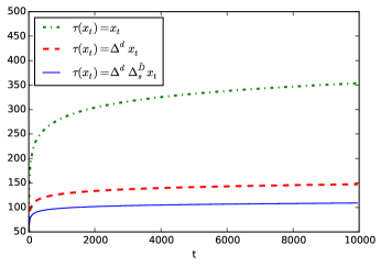
Figure 1: Empirical Regret Bounds

4 Multivariate Methods

Online prediction using multivariate nonstationary models present an additional difficulty due to the notion of cointegration (Section 2). Estimating EC-VARMA models in the static setting is non-trivial in general since the cointegrating rank is unknown and is typically determined by statistical tests (e.g. trace statistic of Johansen [1988]), which again is not realistic in the online setting. We propose a novel online method for cointegrated vector time series that simultaneously updates both the cointegrating matrix (including its rank) and the approximating VAR matrix parameters in order to accurately adapt to the underlying DGP and make predictions.

4.1 Online Prediction for EC-VARMA Models

We generalize the assumptions U1-U4 to the multivariate setting:

• $\mathbf{x}_{t}$ is generated by an EC-VARMA process. The noise sequence $\bm{\varepsilon}_{t}$ of the underlying VARMA process is independent. Also, it satisfies that $\mathbb{E}[\|\bm{\varepsilon}_{t}\|_{2}]<M_{\max}<\infty$.

• We overload notation for the vector case and let $\ell_{t}:\mathbb{R}^{2k}\rightarrow\mathbb{R}$ be a convex loss function with Lipschitz with constant $L>0$.

• We assume the companion matrix $\mathbf{F}$ of the MA lag polynomial is diagonalizable. $\lambda_{\max}$ and $\kappa$ are the same as in assumption U4.

The resulting algorithm is summarized in Algorithm 2, denoted EC-VARMA-OGD. The setup of this algorithm is the same as in Section 3. We overload more notation to generalize Equations 5 and 6. First, we have $\ell_{t}^{M}(\bm{\gamma}):=$

$$\ell_{t}\left(\mathbf{x}_{t},\mathbf{x}_{t-1}+\hat{\Pi}\mathbf{x}_{t-1}+\sum_{{i}=1}^{M}\hat{\Gamma}_{i}\Delta\mathbf{x}_{t-i}\right)$$ (8)

and $f_{t}(\Pi,\Gamma,\bm{\Theta})=$

$$\ell_{t}\left(\mathbf{x}_{t},\mathbf{x}_{t-1}+\Pi\mathbf{x}_{t-1}+\sum_{{i}=1}^{p-1}\Gamma_{i}\Delta\mathbf{x}_{t-i}+\sum_{{i}=1}^{q}\bm{\Theta}_{i}\bm{\varepsilon}_{t-i}\right)$$

where $\bm{\gamma}=\{\hat{\Pi},\hat{\Gamma}_{1},\ldots,\hat{\Gamma}_{M}\}$ are the approximating EC-VAR parameters. The regret as defined in Eq. (7) can be generalized to

$$\text{Regret}=\sum_{{t}=1}^{T}\ell_{t}^{M}(\bm{\gamma}_{t})-\min_{\Pi,\Gamma,\bm{\Theta}\in\mathcal{K}}\sum_{{t}=1}^{T}\mathbb{E}[f_{t}(\Pi,\Gamma,\bm{\Theta})]$$ (9)

where $\mathcal{K}$ is the set of invertible EC-VARMA processes.

To encourage $\hat{\Pi}$ to be low rank, we project it onto $\mathcal{B}(\cdot,\rho)$, which is the nuclear norm ball of radius $\rho$. This involves projecting the singular values of $\hat{\Pi}$ onto an $\ell_{1}$-ball and can be efficiently done [Duchi et al., 2008]. In our framework, this is handled by letting the convex set $\mathcal{E}$ be described as $\{\bm{\gamma}:\|\hat{\Pi}\|_{*}\leq\rho,\|\hat{\Gamma}_{i}\|_{\max}\leq 1,\ i=1,\ldots,M\}$ and plugging it into OGD where projections are made at each iteration. For convenience of notation, let $\mathcal{E}_{\Gamma}=\{\hat{\Gamma}:\|\hat{\Gamma}_{i}\|_{\max}\leq 1,i=1,\ldots M\}$. As in Section 3, $\mathcal{E}$ should be chosen to be large enough to encompass a valid approximation to the true DGP.

Algorithm 2 EC-VARMA-OGD

0:  DGP parameters $p,q$. Horizon $T$. Learning rate $\eta$. Data: $\{\mathbf{x}_{t}\}$.

1:  Set $M=\log_{\lambda_{\max}}\left(\left(2\kappa TLM_{\max}\sqrt{q}\right)^{-1}\right)+p$

2:  Choose $\bm{\gamma}^{(1)}\in\mathcal{E}$ arbitrarily.

3:  for $t=1$ to $T$ do

4:     Predict $\tilde{\mathbf{x}}_{t}=\mathbf{x}_{t-1}+\hat{\Pi}\mathbf{x}_{t-1}+\sum_{{i}=1}^{M}\hat{\Gamma}_{i}\Delta\mathbf{x}_{t-i}$

5:     Observe $\mathbf{x}_{t}$ and receive loss $\ell_{t}^{M}\left(\bm{\gamma}^{(t)}\right)$

6:     $\hat{\Gamma}^{(t+1)}_{i}=\Pi_{\mathcal{E}_{\Gamma}}\left(\hat{\Gamma}^{(t)}_{i}-\eta\nabla_{\Gamma_{i}}\ell_{t}^{M}\left(\bm{\gamma}^{(t)}\right)\right)$

7:     $\hat{\Pi}^{(t+1)}=\Pi_{\mathcal{B}(*,\rho)}\left(\hat{\Pi}^{(t)}-\eta_{t}\nabla_{\Pi}\ell_{t}^{M}\left(\bm{\gamma}^{(t)}\right)\right)$

8:  end for

We present the following regret bound:

Theorem 4.1.

Let $\eta=\frac{D}{G(T)\sqrt{T}}$. Then for any data sequence $\{\mathbf{x}_{t}\}_{t=1}^{T}$ that satisfies assumptions M1-M3, Algorithm 2 generates a sequence $\{\bm{\gamma}_{t}\}$ in which

$$\textrm{Regret}=O\left(DG(T)\sqrt{T}\right)$$

For the remainder of the section, we assume that $\ell_{t}$ is the squared loss and $\|\mathbf{x}_{t}\|_{2}<C(t)=O(\log t)$.

Remark 1: With the above assumptions, the resulting regret bound of EC-VARMA-OGD is $O\left(k^{2}M^{2}\log^{2}(T)\sqrt{T}\right)$.

Remark 2: By setting $\rho=0$ and using $\mathbf{x}_{t}$ in place of $\Delta\mathbf{x}_{t}$ (i.e. not differencing) in Algorithm 2, we effectively use a VARMA process as the DGP and achieve an equivalent regret bound as in the previous remark. Denote this adaptation as VARMA-OGD. However, if the DGP is EC-VARMA, we expect this to empirically perform worse than EC-VARMA-OGD since the latter exploits a valid transformation of the data.

Remark 3: Assume that the DGP is an EC-VARMA process and $\rho=o(1/\log^{2}(T))$. Then the regret bound obtained is $O\left(k^{2}M^{2}\sqrt{T}\right)$. In Section 6, we find that this choice of $\rho$ works well empirically.

5 NonSTOP

Algorithms 1 and 2 assume that the appropriate transformation is known apriori. Typically, statistical tests are used to determine the degree of differencing on a fixed dataset (e.g. Elliot et al. [1996]) and these usually come with assumptions and sample size requirements. In the online setting, these requirements are not realistic and an ideal method must adapt to the incoming data from a possibly time dependent sequence of transformations. We approach this problem by using the online learning with experts (OLE) setup wherein each expert corresponds to a specific transformation (including the identity transform). Specifically, we adapt the (randomized) weighted majority algorithm [Shalev-Shwartz, 2011] as a meta-algorithm to select a transformation at each time step.

More precisely, let $\mathcal{M}$ be the set of experts we consider. The set of experts can either be instantiations of Algorithm 1 or 2. For example, in the univariate setting, we could have $\mathcal{M}=\{\text{ARMA-OGD},\text{ARIMA-OGD},\text{SARIMA-OGD}\}$ with both $d$ and $\tilde{D}$ set to $1$, and in the multivariate setting we can have $\mathcal{M}=\{\text{VARMA-OGD},\text{EC-VARMA-OGD}\}$. We assume that the seasonal period $s$ is known.

Algorithm 3 NonSTOP

0:  DGP parameters $l_{a},l_{m}$. Horizon $T$. Data: $\{x_{t}\}$. Models $\mathcal{M}$. Window size $k$.

1:  Set $\eta=\sqrt{\frac{\log|\mathcal{M}|}{T}}$

2:  Initialize $\bm{w}_{1}=\begin{bmatrix}1&\ldots&1\end{bmatrix}$

3:  for $t=1$ to $T$ do

4:     Set $b_{t}=\max_{\tau\in\{t-k,\ldots.t\},h\in\mathcal{M}}\ell_{\tau}(h),W_{t}=\sum_{h}w_{t}(h)$

5:     Predict using $h_{t}\in\mathcal{M}$, where $h_{t}$ is chosen using probability distribution $\frac{\bm{w}_{t}}{W_{t}}$

6:     For each model in $\mathcal{M}$, run the update according to Algorithm 1.

7:     Update ${w}_{t+1}[h]={w}_{t}[h](1-\eta)^{\frac{\ell_{t}(h)}{b_{t}}}$ for all $h\in\mathcal{M}$

8:  end for

The resulting algorithm refered to as NonSTOP is summarized in Algorithm 3. In each round, the online meta-algorithm randomly selects a prediction from one of its experts. After receiving the loss, it then updates its view about its experts, while the experts themselves are adapting to the data. We scale the loss function with a sliding window maximum such that the losses stay bounded. Since $D,G(T)$, and $\ell_{t}^{M}\left(\bm{\gamma}^{(t)}\right)$ as shown in Algorithm 1 and 2 are now dependent on the specific transformation, we denote this as $D_{h},G_{h}(T),\ell_{t,h}^{M}\left(\bm{\gamma}_{h}^{(t)}\right)$ for a model $h\in\mathcal{M}$. Define Regret = $\sum_{{t}=1}^{T}\mathbb{E}\left[\ell_{t}(h_{t})\right]-\min_{\bm{\alpha},\bm{\beta}\in\mathcal{K}}\sum_{{t}=1}^{T}\mathbb{E}\left[f_{t}(\bm{\alpha},\bm{\beta})\right]$, where $\ell_{t}(h):=\ell_{t,h}^{M}\left(\bm{\gamma}^{(t)}_{h}\right)$. With these definitions in hand, we give the following theorem:

Theorem 5.1.

Define $B_{T}:=\max_{\tau\in\{1,\ldots,t\},h\in\mathcal{M}}\ell_{\tau}(h)$. Then Algorithm 3 plays a sequence of predictions that satisfies

$$\textrm{Regret}=O\left(\max\left\{B_{T},D_{*}G_{*}(T)\right\}\sqrt{T}\right)$$

where $D_{*}=\max_{h}D_{h},\ G_{*}(T)=\max_{h}G_{h}(T)$.

Remark 5.1.1.

When using least squares loss, $B_{T}=O(G_{*}(T))$ and the regret bound defaults to $O\left(D_{*}G_{*}(T)\sqrt{T}\right)$.

6 Empirical Results

In this section, we show empirically the effectiveness of methods described in Sections 3, 4, and 5 on synthetic and real datasets. In each scenario, we use squared loss and plot the log average squared loss vs. iteration. For all experiments, we set $\mathcal{E}=\{\bm{\gamma}:\|\bm{\gamma}\|_{\max}\leq 1\}$, initialize all parameters to 0, and set the sliding window length $k=10$. For all real world datasets, we log transform the time series. Plots of these datasets can be found in the Supplement.

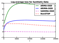
(a) Synthetic data

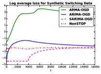
(b) Synthetic switching data

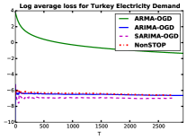
(c) Turkey electricity demand

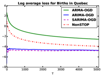
(d) Births in Quebec

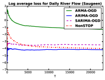
(e) Saugeen River flow

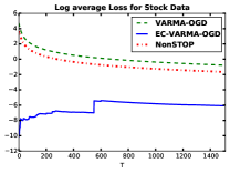
(f) Stock data

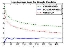
(g) Google flu data

Figure 2: Empirical results for synthetic and real datasets

6.1 Univariate Setting

To illustrate that applying transformations accounting for appropriate nonstationarities results in superior empirical performance, we compare the algorithms given in Table 3. We also include a comparison to NonSTOP to showcase its efficacy in a fully online setting. For each dataset, we assume the seasonal differencing order $\tilde{D}=1$. We set $M=2s$ and $d=1$ for each dataset.

We first simulate 20 synthetic time series with $T=20000$ from the following SARIMA model:

$$\Delta\Delta_{12}x_{t}=(1-0.95L)(1-0.4L^{12})\epsilon_{t}$$ (10)

We run the algorithms on each generated time series and average the log average loss in Figure 2a. As expected, SARIMA-OGD outperforms ARMA-OGD and ARIMA-OGD, converging quickly as it accounts for the appropriate nonstationarities. This behaviour is consistent with our hypothesis that in the absence of an appropriate transformation, existing methods will underperform. NonSTOP gradually adapts and learns to heavily weight the correct transformation (expert) and outperforms ARMA-OGD and ARIMA-OGD.

To showcase the adaptability of NonSTOP, we simulate 20 synthetic time series from Eq. (16) for $4000$ timesteps from a SARIMA model, and then simulate data from an ARIMA model for another $12000$ timesteps. Results are shown in Figure 2b. NonSTOP learns to weight SARIMA-OGD initially, but quickly adapts at $t=4000$ to weight ARIMA-OGD. In fact, at the end of the run, it actually outperforms all experts, showing the power of this online adaptable algorithm.

Next, we consider a dataset that contains daily electricity demand in Turkey. The seasonality in this dataset is biannual. The results of running the algorithms are shown in Figure 2c. Again, SARIMA-OGD accounts for the appropriate nonstationarities and performs the best. ARMA-OGD suffers severely due to not accounting for any nonstationarity. As such, NonSTOP quickly finds that ARMA-OGD is not a reliable expert and performs well in comparison to the other experts. For the daily recorded births in Quebec, there is a weekly seasonality pattern with $s=7$. Figure 2d reveals that the results here are similar to previous datasets. Because NonSTOP starts with an equal weight for each expert, it pays a large penalty for selecting ARMA-OGD in initial iterations. However, it approaches the performance of the other algorithms as it learns to heavily weight the correct transformation.

Lastly, we consider a dataset consisting of daily river flow values from the Saugeen River. This data seems to exhibit a yearly ($s=365$) seasonality pattern (see supplement). The results are plotted in Figure 2e. While accounting for any nonstationarity improves performance, accounting for seasonality actually hurts the performance compared to accounting for only trend. In our experience, ARIMA can sometimes outperform SARIMA even on seemingly seasonal data. Despite this, NonSTOP learns to weight ARIMA-OGD and quickly approaches the best performance. This showcases the efficacy of the NonSTOP algorithm in a fully online setting.

6.2 Multivariate Setting

We collected 7 time series of stock prices from Yahoo Finance of large technology companies, and also included the S&P500 index. By including the S&P500, which is essentially an weighted average of 500 company stock prices, we have partially introduced cointegration into the time series. We set $M=10,\rho=0.5$ and ran all algorithms with the resulting plots in Figure 2f. Accounting for cointegration results in considerably stronger performance. There is a bump in the convergence plot due to a spike in the data (see Supplement). We also evaluated the algorithms on the Google Flu dataset. There are two distinct seasonality patterns: the northern hemisphere countries have flu incidents that peak in one part of the year while the southern hemisphere countries have flu incidents that peak in the other part of the year. Thus, it makes sense to believe that the time series exhibit cointegration. This dataset exhibits yearly seasonality, thus we set $M=60$ to be larger than one seasonal period. We choose $\rho=0.5$ and plot the results are given in Figure 2g. Again, adjusting for the cointegration dramatically increases predictive performance.

On both datasets, NonSTOP pays a penalty for selecting VARMA-OGD in the initial iterations before learning to heavily weight EC-VARMA-OGD. Note that NonSTOP outperforms VARMA-OGD by at least a factor of 3 on the original scale for both datasets.

7 Conclusions and Future Work

We presented general online time series methods that account for nonstationary artifacts in both univariate and multivariate data. If such artifacts are known in advance, we demonstrate that these transformations lead to superior theoretical and empirical performance. Speculating that accounting for nonstationarities reduces correlation in the data, we presented a data dependent regret bound for FTL in the case of squared loss. In the case that the artifacts are unknown, we incorporate a finite set of possible transformations into a OLE framework called NonSTOP that can learn to appropriately weight the correct transformation. We provided empirical results showing the efficacy of our proposed methods. In future work, we plan to explore extensions that hold for more complicated models including long memory models such as ARFIMA.

Appendix A More Background: Companion Matrix

If the MA lag polynomial of a SARIMA process has all of its roots outside of the complex unit circle, then the SARIMA process is defined as invertible. Let $\beta_{i}$ be the scalar coefficients of the MA lag polynomial (recall that this is $\theta(L)\Theta(L^{s})$). Invertibility is equivalent to saying that the companion matrix

$$\mathbf{F}=\begin{bmatrix}-\beta_{1}&-\beta_{2}&\ldots&\ldots&-\beta_{l_{m}}\\ 1&0&\ldots&\ldots&0\\ 0&1&0&\ldots&\vdots\\ \vdots&0&\ddots&\ddots&\vdots\\ 0&\vdots&\vdots&1&0\end{bmatrix}$$

has eigenvalues less than 1 in magnitude. If this is the case, then the underlying ARMA process $\Delta^{d}\Delta^{\tilde{D}}_{s}x_{t}$ can be written as an AR$(\infty)$ process and can be approximated by a finite truncated AR process.

In the multivariate setting, the requirements for invertibility are very similar to the univariate case. For EC-VARMA (and VARMA) processes, we require that $\det\left(\bm{\Theta}(L)\right)$ must have all of its roots outside of the complex unit circle. Again, this is equivalent to saying that the companion matrix has eigenvalues less than 1 in magnitude [Lütkepohl, 2005, Tsay, 2013]. If the process is invertible, then it can be rewritten as a VAR$(\infty)$ process.

Appendix B Proof of Theorem 3.1

We give a proof similar to Anava et al. [2013] and Liu et al. [2016] using our transformation notation, and with the more natural and relaxed assumption of invertibility of the MA process.

Proof.

Step 1: Assume that $\zeta(\tilde{x}_{t})$ is a linear function such as the ones given in Table 2. Then $\{\ell_{t}^{M}\}$ are convex loss functions, and we may invoke [Zinkevich, 2003] with a fixed step size $\eta=\frac{D}{G(T)\sqrt{T}}$:

$$\sum_{{t}=1}^{T}\ell_{t}^{M}(\bm{\gamma}_{t})-\min_{\bm{\gamma}}\sum_{{t}=1}^{T}\ell_{t}^{M}(\bm{\gamma})=O\left(DG(T)\sqrt{T}\right)$$

Note that the proof in [Zinkevich, 2003] uses a constant upper bound $G$ on the gradients. Since we assume $G(T)$ is a monotonically increasing function, the proof in [Zinkevich, 2003] follows through straightforwardly.

Step 2: Let $\bm{\alpha},\bm{\beta}$ denote the parameters of the underlying ARMA$(l_{a},l_{m})$ process. We define a few things:

$$\tau\left(x_{t}^{\infty}(\bm{\alpha},\bm{\beta})\right) =\sum_{{i}=1}^{l_{a}}\alpha_{i}\tau\left(x_{t-i}\right)+\sum_{{i}=1}^{l_{m}}\beta_{i}\left(\tau\left(x_{t-i}\right)-\tau\left(x_{t-i}^{\infty}(\bm{\alpha},\bm{\beta})\right)\right)$$

$$x_{t}^{\infty}(\bm{\alpha},\bm{\beta}) =\zeta\left(\tau\left(x_{t}^{\infty}(\bm{\alpha},\bm{\beta})\right)\right)$$

with initial condition $\tau\left(x_{t}^{\infty}(\bm{\alpha},\bm{\beta})\right)=\tau\left(x_{t}\right)$ for $t<0$. For convenience, assume that we have fixed data $x_{0},\ldots,x_{-h}$ so that $\tau(x_{0}),\ldots,\tau(x_{-l_{a}})$ exists. Denote

$$f_{t}^{\infty}(\bm{\alpha},\bm{\beta})=\ell_{t}\left(x_{t},x_{t}^{\infty}(\bm{\alpha},\bm{\beta})\right)$$

With this definition, we can write $\tau\left(x_{t}^{\infty}(\bm{\alpha},\bm{\beta})\right)=\sum_{{i}=1}^{t+l_{a}}c_{i}(\bm{\alpha},\bm{\beta})\tau\left(x_{t-i}\right)$, i.e. as a growing AR process. Next, we define

$$\tau\left(x_{t}^{m}(\bm{\alpha},\bm{\beta})\right) =\sum_{{i}=1}^{l_{a}}\alpha_{i}\tau\left(x_{t-i}\right)+\sum_{{i}=1}^{l_{m}}\beta_{i}\left(\tau\left(x_{t-i}\right)-\tau\left(x_{t-i}^{m-i}(\bm{\alpha},\bm{\beta})\right)\right)$$

$$x_{t}^{m}(\bm{\alpha},\bm{\beta}) =\zeta\left(\tau\left(x_{t}^{m}(\bm{\alpha},\bm{\beta})\right)\right)$$

with initial condition $\tau\left(x_{t}^{m}(\bm{\alpha},\bm{\beta})\right)=\tau\left(x_{t}\right)$ for $m<0$. We relate $M$ and $m$ with this relation: $M=m+l_{a}$. With this definition, we can write $\tau\left(x_{t}^{m}(\bm{\alpha},\bm{\beta})\right)=\sum_{{i}=1}^{M}\tilde{c}_{i}(\bm{\alpha},\bm{\beta})\tau\left(x_{t-i}\right)$, i.e. as a fixed length AR process. Denote

$$f_{t}^{m}(\bm{\alpha},\bm{\beta})=\ell_{t}\left(x_{t},x_{t}^{m}(\bm{\alpha},\bm{\beta})\right)$$

Let $(\bm{\alpha}^{*},\bm{\beta}^{*})=\operatornamewithlimits{argmin}_{\bm{\alpha},\bm{\beta}\in\mathcal{K}}\sum_{{t}=1}^{T}\mathbb{E}\left[f_{t}(\bm{\alpha},\bm{\beta})\right]$. Recall that the only random part of the expectation is $\varepsilon_{t}$. $x_{t}$ is fixed in this quantity.

Lemma B.1 gives us that

$$\min_{\bm{\gamma}}\sum_{{t}=1}^{T}\ell_{t}^{M}({\bm{\gamma}})\leq\sum_{{t}=1}^{T}f_{t}^{m}(\bm{\alpha}^{*},\bm{\beta}^{*})$$

Lemma B.3 says that choosing $m=\log_{\lambda_{\max}}\left(\left(2\kappa TLM_{\max}\sqrt{l_{m}}\right)^{-1}\right)$ results in

$$\left|\sum_{{t}=1}^{T}\mathbb{E}[f_{t}^{m}(\bm{\alpha}^{*},\bm{\beta}^{*})]-\sum_{{t}=1}^{T}\mathbb{E}[f_{t}^{\infty}(\bm{\alpha}^{*},\bm{\beta}^{*})]\right|=O(1)$$

Lemma B.2 gives us that

$$\left|\sum_{{t}=1}^{T}\mathbb{E}[f_{t}^{\infty}(\bm{\alpha}^{*},\bm{\beta}^{*})]-\sum_{{t}=1}^{T}\mathbb{E}[f_{t}(\bm{\alpha}^{*},\bm{\beta}^{*})]\right|=O(1)$$

Chaining all of these gives us the final result:

$$\sum_{{t}=1}^{T}\ell_{t}^{m}(\bm{\gamma}_{t})-\min_{\bm{\alpha},\bm{\beta}\in\mathcal{K}}\sum_{{t}=1}^{T}\mathbb{E}[f_{t}(\bm{\alpha},\bm{\beta})]=O\left(DG(T)\sqrt{T}\right)$$

∎

Lemma B.1.

For all $m$ and $\{x_{t}\}$ that satisfies the assumptions U1-U4, we have that

$$\min_{\bm{\gamma}}\sum_{{t}=1}^{T}\ell_{t}^{m}({\bm{\gamma}})\leq\sum_{{t}=1}^{T}f_{t}^{m}(\bm{\alpha}^{*},\bm{\beta}^{*})$$

Proof.

We simply set $\gamma_{i}^{*}=\tilde{c}_{i}(\bm{\alpha}^{*},\bm{\beta}^{*})$ and get $\sum_{{t}=1}^{T}\ell_{t}^{m}({\bm{\gamma}}^{*})=\sum_{{t}=1}^{T}f_{t}^{m}(\bm{\alpha}^{*},\bm{\beta}^{*})$. Thus, the minimum holds trivially. Note that we assume ${\bm{\gamma}}^{*}\in\mathcal{E}.$ ∎

Lemma B.2.

For any data sequence $\{x_{t}\}$ that satisfies the assumptions U1-U4, it holds that

$$\left|\sum_{{t}=1}^{T}\mathbb{E}[f_{t}^{\infty}(\bm{\alpha}^{*},\bm{\beta}^{*})]-\sum_{{t}=1}^{T}\mathbb{E}[f_{t}(\bm{\alpha}^{*},\bm{\beta}^{*})]\right|=O(1)$$

Proof.

Let $(\bm{\alpha}^{\prime},\bm{\beta}^{\prime})$ denote the parameters that generated the signal. Thus,

$$f_{t}(\bm{\alpha}^{\prime},\bm{\beta}^{\prime})=\ell_{t}(x_{t},x_{t}-\varepsilon_{t})$$

for all $t$. Since $\varepsilon_{t}$ is independent of $\varepsilon_{1},\ldots,\varepsilon_{t-1}$, the best prediction at time $t$ will cause a loss of at least $\mathbb{E}[\ell_{t}(x_{t},x_{t}-\varepsilon_{t})].$ Since $\mathbb{E}[\varepsilon_{t}]=0$ and $\ell_{t}$ is convex, it follows that $(\bm{\alpha}^{*},\bm{\beta}^{*})=(\bm{\alpha}^{\prime},\bm{\beta}^{\prime})$ and that

$$f_{t}(\bm{\alpha}^{*},\bm{\beta}^{*})=\ell_{t}(x_{t},x_{t}-\varepsilon_{t})$$

We define a few things first. Let

$$y_{t}=\tau\left(x_{t}\right)-\tau\left(x_{t}^{\infty}(\bm{\alpha}^{*},\bm{\beta}^{*})\right)-\varepsilon_{t},\ \ \ \ \mathbf{y}_{t}=\begin{bmatrix}y_{t}\\ y_{t-1}\\ \vdots\\ y_{t-q+1}\end{bmatrix}$$

WLOG (and by assumption), we can assume that $\mathbb{E}\left[\|\mathbf{y}_{0}\|_{2}\right]\leq\rho$, where $\rho$ is some positive constant. Next we show that

$$\mathbb{E}[|y_{t}|]=\mathbb{E}\left[|\tau\left(x_{t}\right)-\tau\left(x_{t}^{\infty}(\bm{\alpha}^{*},\bm{\beta}^{*})\right)-\varepsilon_{t}|\right]\leq\kappa\lambda_{\max}^{t}\rho$$

We have that

$$\tau\left(x_{t}\right)-\tau\left(x_{t}^{\infty}(\bm{\alpha}^{*},\bm{\beta}^{*})\right)-\varepsilon_{t}= \sum_{{i}=1}^{l_{a}}\alpha_{i}^{*}\tau\left(x_{t-i}\right)+\sum_{{i}=1}^{l_{m}}\beta_{i}^{*}\varepsilon_{t-i}+\varepsilon_{t}$$

$$-\sum_{{i}=1}^{l_{a}}\alpha_{i}^{*}\tau\left(x_{t-i}\right)-\sum_{{i}=1}^{l_{m}}\beta_{i}^{*}\left(\tau\left(x_{t-i}\right)-\tau\left(x_{t-i}^{\infty}(\bm{\alpha}^{*},\bm{\beta}^{*})\right)\right)-\varepsilon_{t}$$

$$= -\sum_{{i}=1}^{l_{m}}\beta_{i}^{*}\left(\tau\left(x_{t-i}\right)-\tau\left(x_{t-i}^{\infty}(\bm{\alpha}^{*},\bm{\beta}^{*})\right)-\varepsilon_{t-i}\right)$$

which shows that $y_{t}=-\sum_{{i}=1}^{l_{m}}\beta_{i}^{*}y_{t-i}$. The companion matrix to this difference equation is exactly $\mathbf{F}$ as defined in Eq. A. Thus,

$$\mathbf{y}_{t}=\mathbf{F}\mathbf{y}_{t-1}$$

Next, we note that

$$|y_{t}| \leq\|\mathbf{y}_{t}\|_{2}=\|\mathbf{F}\mathbf{y}_{t-1}\|_{2}$$

$$=\|\mathbf{F}^{2}\mathbf{y}_{t-2}\|_{2}$$

$$=\|\mathbf{F}^{t}\mathbf{y}_{0}\|_{2}$$

$$=\|\mathbf{T}\Lambda^{t}\mathbf{T}^{-1}\mathbf{y}_{0}\|_{2}$$

$$\leq\|\mathbf{T}\|_{2}\|\mathbf{T}^{-1}\|_{2}\|\Lambda^{t}\|_{2}\|\mathbf{y}_{0}\|_{2}$$

$$=\frac{\sigma_{\max}(\mathbf{T})}{\sigma_{\min}(\mathbf{T})}\lambda_{\max}^{t}\|\mathbf{y}_{0}\|_{2}$$

$$\leq\kappa\lambda_{\max}^{t}\|\mathbf{y}_{0}\|_{2}$$

Taking the expectation gives us $\mathbb{E}[|y_{t}|]\leq\kappa\lambda_{\max}^{t}\mathbb{E}\left[\|\mathbf{y}_{0}\|_{2}\right]\leq\kappa\lambda_{\max}^{t}\rho.$

Now we combine this with the Lipschitz continuity of $\ell_{t}$ to get

$$\left|\mathbb{E}\left[f_{t}^{\infty}(\bm{\alpha}^{*},\bm{\beta}^{*})\right]-\mathbb{E}\left[f_{t}(\bm{\alpha}^{*},\bm{\beta}^{*})\right]\right| =\left|\mathbb{E}\left[\ell_{t}(x_{t},x_{t}^{\infty}(\bm{\alpha}^{*},\bm{\beta}^{*}))\right]-\mathbb{E}\left[\ell_{t}(x_{t},x_{t}-\varepsilon_{t})\right]\right|$$

$$\leq\mathbb{E}\left[|\ell_{t}(x_{t},x_{t}^{\infty}(\bm{\alpha}^{*},\bm{\beta}^{*}))-\ell_{t}(x_{t},x_{t}-\varepsilon_{t})|\right]$$

$$\leq L\cdot\mathbb{E}\left[|x_{t}-x_{t}^{\infty}(\bm{\alpha}^{*},\bm{\beta}^{*})-\varepsilon_{t}|\right]$$

$$=L\cdot\mathbb{E}\left[|\tau\left(x_{t}\right)-\tau\left(x_{t}^{\infty}(\bm{\alpha}^{*},\bm{\beta}^{*})\right)-\varepsilon_{t}|\right]$$

$$\leq\kappa L\rho\lambda_{\max}^{t}$$

where we used Jensen’s inequality in the first inequality. Note that we also assume $x_{t}-\tilde{x}_{t}=\zeta(\tau(x_{t}))-\zeta(\tau(\tilde{x}_{t}))=\tau(x_{t})-\tau(\tilde{x}_{t})$. This holds true for the transformations given in Table 2. Summing this from $t=1$ to $T$ gives us the result. ∎

Lemma B.3.

For any data sequence $\{x_{t}\}$ that satisfies the assumptions U1-U4, it holds that

$$\left|\sum_{{t}=1}^{T}\mathbb{E}\left[f_{t}^{m}(\bm{\alpha}^{*},\bm{\beta}^{*})\right]-\sum_{{t}=1}^{T}\mathbb{E}\left[f_{t}^{\infty}(\bm{\alpha}^{*},\bm{\beta}^{*})\right]\right|=O(1)$$

if we choose $m=\log_{\lambda_{\max}}\left((2\kappa TLM_{\max}\sqrt{l_{m}})^{-1}\right).$

Proof.

Fix $t$. Note that for $m<0$,

$$|\tau\left(x_{t}^{m}(\bm{\alpha}^{*},\bm{\beta}^{*})\right)-\tau\left(x_{t}^{\infty}(\bm{\alpha}^{*},\bm{\beta}^{*})\right)| =|\tau\left(x_{t}\right)-\tau\left(x_{t}^{\infty}(\bm{\alpha}^{*},\bm{\beta}^{*})\right)|$$

$$\leq|\tau\left(x_{t}\right)-\tau\left(x_{t}^{\infty}(\bm{\alpha}^{*},\bm{\beta}^{*})\right)-\varepsilon_{t}|+|\varepsilon_{t}|$$

The right hand side of the inequality is simply $|y_{t}|+|\varepsilon_{t}|$, where $y_{t}$ is as defined in Lemma B.2. By assumption, $\mathbb{E}[|\varepsilon_{t}|]<M_{\max}$. Assume that $M_{\max}$ is large enough such that $\mathbb{E}[|y_{t}|]\leq M_{\max}$. This is a valid assumption since it is decaying exponentially as proved in Lemma B.2. It is important to note that $\tau\left(x_{t}^{m}(\bm{\alpha},\bm{\beta})\right)$ and $\tau\left(x_{t}^{\infty}(\bm{\alpha},\bm{\beta})\right)$ have no randomness in them since $\tau$ is deterministic. Thus, for $m<0$,

$$|\tau\left(x_{t}^{m}(\bm{\alpha}^{*},\bm{\beta}^{*})\right)-\tau\left(x_{t}^{\infty}(\bm{\alpha}^{*},\bm{\beta}^{*})\right)| =\mathbb{E}\left[|\tau\left(x_{t}^{m}(\bm{\alpha}^{*},\bm{\beta}^{*})\right)-\tau\left(x_{t}^{\infty}(\bm{\alpha}^{*},\bm{\beta}^{*})\right)|\right]$$

$$=\mathbb{E}\left[|\tau\left(x_{t}\right)-\tau\left(x_{t}^{\infty}(\bm{\alpha}^{*},\bm{\beta}^{*})\right)|\right]$$

$$\leq\mathbb{E}[|y_{t}|+|\varepsilon_{t}|]$$

$$\leq 2M_{\max}$$

Squaring both sides of the inequality results in

$$(\tau\left(x_{t}^{m}(\bm{\alpha}^{*},\bm{\beta}^{*})\right)-\tau\left(x_{t}^{\infty}(\bm{\alpha}^{*},\bm{\beta}^{*})\right))^{2}\leq 4M_{\max}^{2}$$

Next, we define

$$z_{t}^{m}=\tau\left(x_{t}^{m}(\bm{\alpha}^{*},\bm{\beta}^{*})\right)-\tau\left(x_{t}^{\infty}(\bm{\alpha}^{*},\bm{\beta}^{*})\right),\ \ \ \ \mathbf{z}_{t}^{m}=\begin{bmatrix}z_{t}^{m}\\ z_{t-1}^{m-1}\\ \vdots\\ z_{t-q+1}^{m-q+1}\end{bmatrix}$$

We have that

$$\tau\left(x_{t}^{m}(\bm{\alpha}^{*},\bm{\beta}^{*})\right)-\tau\left(x_{t}^{\infty}(\bm{\alpha}^{*},\bm{\beta}^{*})\right)= \sum_{{i}=1}^{l_{a}}\alpha^{*}_{i}\tau\left(x_{t-i}\right)+\sum_{{i}=1}^{l_{m}}\beta_{i}^{*}(\tau\left(x_{t-i}\right)-\tau\left(x_{t-i}^{m-i}(\bm{\alpha}^{*},\bm{\beta}^{*})\right))$$

$$-\sum_{{i}=1}^{l_{a}}\alpha^{*}_{i}\tau\left(x_{t-i}\right)-\sum_{{i}=1}^{l_{m}}\beta^{*}_{i}(\tau\left(x_{t-i}\right)-\tau\left(x_{t-i}^{\infty}(\bm{\alpha}^{*},\bm{\beta}^{*})\right))$$

$$= -\sum_{{i}=1}^{l_{m}}\beta^{*}_{i}\left(\tau\left(x_{t-i}^{m-i}(\bm{\alpha}^{*},\bm{\beta}^{*})\right)-\tau\left(x_{t-i}^{\infty}(\bm{\alpha}^{*},\bm{\beta}^{*})\right)\right)$$

Thus, $z_{t}^{m}=-\sum_{{i}=1}^{l_{m}}\beta^{*}_{i}z_{t-i}^{m-i}$. The companion matrix to this difference equation is exactly $\mathbf{F}$ as defined in Eq. A. Thus,

$$\mathbf{z}_{t}^{m}=\mathbf{F}\mathbf{z}_{t-1}^{m-1}$$

We have that

$$|z_{t}^{m}| \leq\|\mathbf{z}_{t}^{m}\|_{2}=\|\mathbf{F}\mathbf{z}_{t-1}^{m-1}\|_{2}$$

$$=\|\mathbf{F}^{2}\mathbf{z}_{t-2}^{m-2}\|_{2}$$

$$=\|\mathbf{F}^{m}\mathbf{z}_{t-m}^{0}\|_{2}$$

$$=\|\mathbf{T}\Lambda^{m}\mathbf{T}^{-1}\mathbf{z}_{t-m}^{0}\|_{2}$$

$$\leq\|\mathbf{T}\|_{2}\|\mathbf{T}^{-1}\|_{2}\|\Lambda^{m}\|_{2}\|\mathbf{z}_{t-m}^{0}\|_{2}$$

$$=\frac{\sigma_{\max}(\mathbf{T})}{\sigma_{\min}(\mathbf{T})}\lambda_{\max}^{m}\sqrt{\sum_{i=0}^{l_{m}-1}(z_{t-m-i}^{-i})^{2}}$$

$$\leq\kappa\lambda_{\max}^{m}\sqrt{q4M_{\max}^{2}}$$

$$=\kappa\lambda_{\max}^{m}2M_{\max}\sqrt{l_{m}}$$

Now we combine this with the Lipschitz continuity of $\ell_{t}$ to get

$$\left|\mathbb{E}[f_{t}^{m}(\bm{\alpha}^{*},\bm{\beta}^{*})]-\mathbb{E}[f_{t}^{\infty}(\bm{\alpha}^{*},\bm{\beta}^{*})]\right| =\left|\mathbb{E}[\ell_{t}(x_{t},x_{t}^{m}(\bm{\alpha}^{*},\bm{\beta}^{*}))]-\mathbb{E}[\ell_{t}(x_{t},x_{t}^{\infty}(\bm{\alpha}^{*},\bm{\beta}^{*}))]\right|$$

$$\leq\mathbb{E}[\left|\ell_{t}(x_{t},x_{t}^{m}(\bm{\alpha}^{*},\bm{\beta}^{*}))-\ell_{t}(x_{t},x_{t}^{\infty}(\bm{\alpha}^{*},\bm{\beta}^{*}))\right|]$$

$$\leq L\cdot\mathbb{E}[|x_{t}^{m}(\bm{\alpha}^{*},\bm{\beta}^{*})-x_{t}^{\infty}(\bm{\alpha}^{*},\bm{\beta}^{*})|]$$

$$=L\cdot|\tau\left(x_{t}^{m}(\bm{\alpha}^{*},\bm{\beta}^{*})\right)-\tau\left(x_{t}^{\infty}(\bm{\alpha}^{*},\bm{\beta}^{*})\right)|$$

$$\leq 2\kappa LM_{\max}\sqrt{l_{m}}\lambda_{\max}^{m}$$

where in the first inequality we used Jensen’s inequality and we again used the assumption that $x_{t}-\tilde{x}_{t}=\tau(x_{t})-\tau(\tilde{x}_{t})$.

Summing this quantity from $t=1$ to $T$ gives us the result:

$$\left|\sum_{{t}=1}^{T}\mathbb{E}[f_{t}^{\infty}(\bm{\alpha}^{*},\bm{\beta}^{*})]-\sum_{{t}=1}^{T}\mathbb{E}[f_{t}^{m}(\bm{\alpha}^{*},\bm{\beta}^{*})]\right|\leq 2\kappa TLM_{\max}\sqrt{l_{m}}\lambda_{\max}^{m}$$

Choosing $m=\log_{\lambda_{\max}}\left((2\kappa TLM_{max}\sqrt{l_{m}})^{-1}\right)$ gives us the desired $O(1)$ property. ∎

Appendix C Proof of Theorem 4.1

Proof.

We again produce a proof of very similar structure to Anava et al. [2013] and Liu et al. [2016]. We first need to redefine a few things for the vector case. Let $D=\sup_{\bm{\gamma}_{1},\bm{\gamma}_{2}\in\mathcal{K}}\|\bm{\gamma}_{1}-\bm{\gamma}_{2}\|_{F}$, and $\|\nabla_{\bm{\gamma}}\ell_{t}^{m}(\bm{\gamma})\|_{F}\leq G(T)$.

Step 1: Since $\{\ell_{t}^{M}\}$ are convex loss functions, we may invoke [Zinkevich, 2003] with a fixed step size $\eta=\frac{D}{G(T)\sqrt{T}}$:

$$\sum_{{t}=1}^{T}\ell_{t}^{M}(\bm{\gamma}_{t})-\min_{\bm{\gamma}}\sum_{{t}=1}^{T}\ell_{t}^{M}(\bm{\gamma})=O\left(DG(T)\sqrt{T}\right)$$

Again, we note that the proof in [Zinkevich, 2003] uses a constant upper bound $G$ on the gradients. Since we assume $G(T)$ is a monotonically increasing function, the proof in [Zinkevich, 2003] follows through straightforwardly.

Step 2: Next we define a few things in the same vein as in the proof of Theorem 3.1. Let

$$\Delta\mathbf{x}_{t}^{\infty}(\Pi,\Gamma,\bm{\Theta}) =\Pi\mathbf{x}_{t-1}+\sum_{{i}=1}^{p-1}\Gamma_{i}\Delta\mathbf{x}_{t-i}+\sum_{{i}=1}^{q}\bm{\Theta}_{i}\left(\Delta\mathbf{x}_{t-i}-\Delta\mathbf{x}_{t-i}^{\infty}(\Pi,\Gamma,\bm{\Theta})\right)$$

$$\mathbf{x}_{t}^{\infty}(\Pi,\Gamma,\bm{\Theta}) =\Delta\mathbf{x}_{t}^{\infty}(\Pi,\Gamma,\bm{\Theta})+\mathbf{x}_{t-1}$$

$$f_{t}^{\infty}(\Pi,\Gamma,\bm{\Theta}) =\ell_{t}\left(\mathbf{x}_{t},\ \mathbf{x}_{t}^{\infty}\left(\Pi,\Gamma,\bm{\Theta}\right)\right)$$

with initial condition $\Delta\mathbf{x}_{t}^{\infty}(\Pi,\Gamma,\bm{\Theta})=\Delta\mathbf{x}_{t}$ for all $t<0$. Note that we are assuming that we have fixed data $\mathbf{x}_{0},\ldots,\mathbf{x}_{-p}$. With this definition, we can write $\Delta\mathbf{x}_{t}^{\infty}(\Pi,\Gamma,\bm{\Theta})=c_{0}(\Pi,\Gamma,\bm{\Theta})\mathbf{x}_{t-1}+\sum_{{i}=1}^{t+p-1}c_{i}(\Pi,\Gamma,\bm{\Theta})\Delta\mathbf{x}_{t-i}$, i.e. as a growing AR process. This is because we can undo the reparameterization and write $\Delta\mathbf{x}_{t}$ in its original VARMA process form

$$\mathbf{x}_{t}^{\infty}(\Pi,\Gamma,\Theta) =\sum_{{i}=1}^{p}\mathbf{A}_{i}\mathbf{x}_{t-i}+\sum_{{i}=1}^{q}\bm{\Theta}_{i}\left(\mathbf{x}_{t-i}-\mathbf{x}_{t-i}^{\infty}(\Pi,\Gamma,\Theta)\right)$$

$$=\sum_{{i}=1}^{t+p}c_{i}(\mathbf{A},\Theta)\mathbf{x}_{t-i}$$

as shown in the proof of Algorithm 1. Using the error corrected reparameterization here results in

$$\Delta\mathbf{x}_{t}^{\infty}(\Pi,\Gamma,\Theta)=c_{0}(\Pi,\Gamma,\Theta)\mathbf{x}_{t-1}+\sum_{{i}=1}^{t+p-1}c_{i}(\Pi,\Gamma,\Theta)\Delta\mathbf{x}_{t-i}$$

Furthermore, we define

$$\Delta\mathbf{x}_{t}^{m}(\Pi,\Gamma,\bm{\Theta}) =\Pi\mathbf{x}_{t-1}+\sum_{{i}=1}^{p-1}\Gamma_{i}\Delta\mathbf{x}_{t-i}+\sum_{{i}=1}^{q}\bm{\Theta}_{i}\left(\Delta\mathbf{x}_{t-i}-\Delta\mathbf{x}_{t-i}^{m-i}(\Pi,\Gamma,\bm{\Theta})\right)$$

$$\mathbf{x}_{t}^{m}(\Pi,\Gamma,\bm{\Theta}) =\Delta\mathbf{x}_{t}^{m}(\Pi,\Gamma,\bm{\Theta})+\mathbf{x}_{t-1}$$

$$f_{t}^{m}(\Pi,\Gamma,\bm{\Theta}) =\ell_{t}(\mathbf{x}_{t},\ \mathbf{x}_{t}^{m}(\Pi,\Gamma,\bm{\Theta}))$$

with initial condition $\Delta\mathbf{x}_{t}^{m}(\Pi,\Gamma,\bm{\Theta})=\Delta\mathbf{x}_{t}$ for all $m<0$. We relate $M=m+p-1$. With this definition, we can write $\Delta\mathbf{x}_{t}^{m}(\Pi,\Gamma,\bm{\Theta})=\tilde{c}_{0}(\Pi,\Gamma,\bm{\Theta})\mathbf{x}_{t-1}+\sum_{{i}=1}^{M}\tilde{c}_{i}(\Pi,\Gamma,\bm{\Theta})\Delta\mathbf{x}_{t-i}$ by using similar rearrangement arguments as shown above.

Lastly, we define

$$(\Pi^{*},\Gamma^{*},\bm{\Theta}^{*})=\operatornamewithlimits{argmin}_{\Pi,\Gamma,\bm{\Theta}}\sum_{{t}=1}^{T}\mathbb{E}[f_{t}(\Pi,\Gamma,\bm{\Theta})]$$

Recall that $\mathbf{x}_{t}$ is fixed in the expectation.

Lemma C.1 gives us that

$$\min_{\bm{\gamma}}\sum_{{t}=1}^{T}\ell_{t}^{M}(\bm{\gamma})\leq\sum_{{t}=1}^{T}f_{t}^{m}(\Pi^{*},\Gamma^{*},\bm{\Theta}^{*})$$

Lemma C.3 says that choosing $m=\log_{\lambda_{\max}}\left(\left(2\kappa TLM_{\max}\sqrt{q}\right)^{-1}\right)$ results in

$$\left|\sum_{{t}=1}^{T}\mathbb{E}[f_{t}^{m}(\Pi^{*},\Gamma^{*},\bm{\Theta}^{*})]-\sum_{{t}=1}^{T}\mathbb{E}[f_{t}^{\infty}(\Pi^{*},\Gamma^{*},\bm{\Theta}^{*})]\right|=O(1)$$

Lemma C.2 gives us that

$$\left|\sum_{{t}=1}^{T}\mathbb{E}[f_{t}^{\infty}(\Pi^{*},\Gamma^{*},\bm{\Theta}^{*})]-\sum_{{t}=1}^{T}\mathbb{E}[f_{t}(\Pi^{*},\Gamma^{*},\bm{\Theta}^{*})]\right|=O(1)$$

Chaining all of these gives us the final result:

$$\sum_{{t}=1}^{T}\ell_{t}^{M}(\bm{\gamma}_{t})-\min_{\Pi,\Gamma,\bm{\Theta}}\sum_{{t}=1}^{T}\mathbb{E}[f_{t}(\Pi,\Gamma,\bm{\Theta})]=O\left(DG(T)\sqrt{T}\right)$$

∎

Lemma C.1.

For all $m$ and $\{\mathbf{x}_{t}\}$ that satisfies assumptions M1-M3, we have that

$$\min_{\bm{\gamma}}\sum_{{t}=1}^{T}\ell_{t}^{m}(\bm{\gamma})\leq\sum_{{t}=1}^{T}f_{t}^{m}(\Pi^{*},\Gamma^{*},\bm{\Theta}^{*})$$

Proof.

Recall that $\bm{\gamma}=\{\tilde{\Pi},\tilde{\Gamma}_{i},\ i=1,\ldots,M\}$ We simply set $\tilde{\Pi}^{*}=\tilde{c}_{0}(\Pi^{*},\Gamma^{*},\bm{\Theta}^{*}),\ \tilde{\Gamma}_{i}^{*}=\tilde{c}_{i}(\Pi^{*},\Gamma^{*},\bm{\Theta}^{*})$ and let that be denoted by $\bm{\gamma}^{*}$. Thus, we get $\sum_{{t}=1}^{T}\ell_{t}^{M}(\bm{\gamma}^{*})=\sum_{{t}=1}^{T}f_{t}^{m}(\Pi^{*},\Gamma^{*},\bm{\Theta}^{*})$. Thus, the minimum holds trivially. Note that we assume $\bm{\gamma}^{*}\in\mathcal{E}$. ∎

Lemma C.2.

For any data sequence $\{\mathbf{x}_{t}\}_{t=1}^{T}$ that satisfies assumptions M1-M5, it holds that

$$\left|\sum_{{t}=1}^{T}\mathbb{E}[f_{t}^{\infty}(\Pi^{*},\Gamma^{*},\bm{\Theta}^{*})]-\sum_{{t}=1}^{T}\mathbb{E}[f_{t}(\Pi^{*},\Gamma^{*},\bm{\Theta}^{*})]\right|=O(1)$$

Proof.

We start the proof in the same exact way that Anava does. Let $(\Pi^{\prime},\Gamma^{\prime},\bm{\Theta}^{\prime})$ denote the parameters that generated the signal. Thus,

$$f_{t}(\Pi^{\prime},\Gamma^{\prime},\bm{\Theta}^{\prime})=\ell_{t}(\mathbf{x}_{t},\mathbf{x}_{t}-\bm{\varepsilon}_{t})$$

for all $t$. Since $\bm{\varepsilon}_{t}$ is independent of $\bm{\varepsilon}_{1},\ldots,\bm{\varepsilon}_{t-1}$, the best prediction at time $t$ will cause a loss of at least $\mathbb{E}[\ell_{t}(\mathbf{x}_{t},\mathbf{x}_{t}-\bm{\varepsilon}_{t})].$ Since $\mathbb{E}[\bm{\varepsilon}_{t}]=0$ and $\ell_{t}$ is convex, it follows that $(\Pi^{*},\Gamma^{*},\bm{\Theta}^{*})=(\Pi^{\prime},\Gamma^{\prime},\bm{\Theta}^{\prime})$ and that

$$f_{t}(\Pi^{*},\Gamma^{*},\bm{\Theta}^{*})=\ell_{t}(\mathbf{x}_{t},\mathbf{x}_{t}-\bm{\varepsilon}_{t})$$

We define a few things first. Let

$$\mathbf{y}_{t}=\Delta\mathbf{x}_{t}-\Delta\mathbf{x}_{t}^{\infty}(\Pi^{*},\Gamma^{*},\bm{\Theta}^{*})-\bm{\varepsilon}_{t},\ \ \ \ \mathbf{Y}_{t}=\begin{bmatrix}\mathbf{y}_{t}\\ \mathbf{y}_{t-1}\\ \vdots\\ \mathbf{y}_{t-q+1}\end{bmatrix}$$

(note the overloading from previous sections) By assumption, we can assume that $\mathbb{E}\left[\|\mathbf{Y}_{0}\|_{2}\right]\leq\rho$, where $\rho$ is some positive constant. Next we show that

$$\mathbb{E}[\|\mathbf{y}_{t}\|_{2}]=\mathbb{E}\left[\|\Delta\mathbf{x}_{t}-\Delta\mathbf{x}_{t}^{\infty}(\Pi^{*},\Gamma^{*},\bm{\Theta}^{*})-\bm{\varepsilon}_{t}\|_{2}\right]\leq\kappa\lambda_{\max}^{t}\rho$$

We have that

$$\Delta\mathbf{x}_{t}-\Delta\mathbf{x}_{t}^{\infty}(\Pi^{*},\Gamma^{*},\bm{\Theta}^{*})-\bm{\varepsilon}_{t}= \ \ \ \Pi^{*}\mathbf{x}_{t-1}+\sum_{{i}=1}^{p-1}\Gamma_{i}^{*}\Delta\mathbf{x}_{t-i}+\sum_{{i}=1}^{q}\bm{\Theta}_{i}^{*}\bm{\varepsilon}_{t-i}+\bm{\varepsilon}_{t}$$

$$-\Pi^{*}\mathbf{x}_{t-1}-\sum_{{i}=1}^{p-1}\Gamma_{i}^{*}\Delta\mathbf{x}_{t-i}-\sum_{{i}=1}^{q}\bm{\Theta}_{i}^{*}\left(\Delta\mathbf{x}_{t-i}-\Delta\mathbf{x}_{t-i}^{\infty}(\Pi^{*},\Gamma^{*},\bm{\Theta}^{*})\right)-\bm{\varepsilon}_{t}$$

$$= -\sum_{{i}=1}^{q}\bm{\Theta}_{i}^{*}\left(\Delta\mathbf{x}_{t-i}-\Delta\mathbf{x}_{t-i}^{\infty}(\Pi^{*},\Gamma^{*},\bm{\Theta}^{*})-\bm{\varepsilon}_{t-i}\right)$$

which shows that $\mathbf{y}_{t}=-\sum_{{i}=1}^{q}\bm{\Theta}_{i}^{*}\mathbf{y}_{t-i}$. The companion matrix to this difference equation is $\mathbf{F}$. Thus,

$$\mathbf{Y}_{t}=\mathbf{F}\mathbf{Y}_{t-1}$$

Next, we note that

$$\|\mathbf{y}_{t}\|_{2} \leq\|\mathbf{Y}_{t}\|_{2}=\|\mathbf{F}\mathbf{Y}_{t-1}\|_{2}$$

$$=\|\mathbf{F}^{2}\mathbf{Y}_{t-2}\|_{2}$$

$$=\|\mathbf{F}^{t}\mathbf{Y}_{0}\|_{2}$$

$$=\|\mathbf{T}\Lambda^{t}\mathbf{T}^{-1}\mathbf{Y}_{0}\|_{2}$$

$$\leq\|\mathbf{T}\|_{2}\|\mathbf{T}^{-1}\|_{2}\|\Lambda^{t}\|_{2}\|\mathbf{Y}_{0}\|_{2}$$

$$=\frac{\sigma_{\max}(\mathbf{T})}{\sigma_{\min}(\mathbf{T})}\lambda_{\max}^{t}\|\mathbf{Y}_{0}\|_{2}$$

$$\leq\kappa\lambda_{\max}^{t}\|\mathbf{Y}_{0}\|_{2}$$

Taking the expectation gives us $\mathbb{E}[\|\mathbf{y}_{t}\|_{2}]\leq\kappa(1-\varepsilon)^{t}\mathbb{E}\left[\|\mathbf{Y}_{0}\|_{2}\right]\leq\kappa\lambda_{\max}^{t}\rho.$

Now we combine this with the Lipschitz continuity of $\ell_{t}$ to get

$$\left|\mathbb{E}\left[f_{t}^{\infty}(\Pi^{*},\Gamma^{*},\bm{\Theta}^{*})\right]-\mathbb{E}\left[f_{t}(\Pi^{*},\Gamma^{*},\bm{\Theta}^{*})\right]\right| =\left|\mathbb{E}\left[\ell_{t}(\mathbf{x}_{t},\mathbf{x}_{t}^{\infty}(\Pi^{*},\Gamma^{*},\bm{\Theta}^{*}))\right]-\mathbb{E}\left[\ell_{t}(\mathbf{x}_{t},\mathbf{x}_{t}-\bm{\varepsilon}_{t})\right]\right|$$

$$\leq\mathbb{E}\left[|\ell_{t}(\mathbf{x}_{t},\mathbf{x}_{t}^{\infty}(\Pi^{*},\Gamma^{*},\bm{\Theta}^{*}))-\ell_{t}(\mathbf{x}_{t},\mathbf{x}_{t}-\bm{\varepsilon}_{t})|\right]$$

$$\leq L\cdot\mathbb{E}\left[\|\mathbf{x}_{t}-\mathbf{x}_{t}^{\infty}(\Pi^{*},\Gamma^{*},\bm{\Theta}^{*})-\varepsilon_{t}\|_{2}\right]$$

$$=L\cdot\mathbb{E}\left[\|\Delta\mathbf{x}_{t}-\Delta\mathbf{x}_{t}^{\infty}(\Pi^{*},\Gamma^{*},\bm{\Theta}^{*})-\varepsilon_{t}\|_{2}\right]$$

$$\leq\kappa L\rho\lambda_{\max}^{t}$$

where we used Jensen’s inequality in the first inequality. Summing this from $t=1$ to $T$ gives us the result. ∎

Lemma C.3.

For any data sequence $\{x_{t}\}_{t=1}^{T}$ that satisfies assumptions M1-M3, it holds that

$$\left|\sum_{{t}=1}^{T}\mathbb{E}\left[f_{t}^{m}(\Pi^{*},\Gamma^{*},\bm{\Theta}^{*})\right]-\sum_{{t}=1}^{T}\mathbb{E}\left[f_{t}^{\infty}(\Pi^{*},\Gamma^{*},\bm{\Theta}^{*})\right]\right|=O(1)$$

if we choose $m=\log_{\lambda_{\max}}\left((2\kappa TLM_{\max}\sqrt{q})^{-1}\right).$

Proof.

Fix $t$. Note that for $m<0$,

$$|\Delta\mathbf{x}_{t}^{m}(\Pi^{*},\Gamma^{*},\bm{\Theta}^{*})-\Delta\mathbf{x}_{t}^{\infty}(\Pi^{*},\Gamma^{*},\bm{\Theta}^{*})| =|\Delta\mathbf{x}_{t}-\Delta\mathbf{x}_{t}^{\infty}(\Pi^{*},\Gamma^{*},\bm{\Theta}^{*})|$$

$$\leq|\Delta\mathbf{x}_{t}-\Delta\mathbf{x}_{t}^{\infty}(\Pi^{*},\Gamma^{*},\bm{\Theta}^{*})-\bm{\varepsilon}_{t}|+|\bm{\varepsilon}_{t}|$$

The right hand side of the inequality is simply $\|\mathbf{y}_{t}\|_{2}+\|\bm{\varepsilon}_{t}\|_{2}$, where $\mathbf{y}_{t}$ is as defined in Lemma C.2. By assumption, $\mathbb{E}[\|\bm{\varepsilon}_{t}\|_{2}]<M_{\max}$. Assume that $M_{\max}$ is large enough such that $\mathbb{E}[\|\mathbf{y}_{t}\|_{2}]\leq M_{\max}$. This is a valid assumption since it is decaying exponentially as proved in Lemma C.2. It is important to note that $\Delta\mathbf{x}_{t}^{m}(\Pi,\Gamma,\bm{\Theta})$ and $\Delta\mathbf{x}_{t}^{\infty}(\Pi,\Gamma,\bm{\Theta})$ have no randomness in them (recall that they can be written as a linear combination of past values of the realized data sequence $\Delta\mathbf{x}_{t}$). Thus, for $m<0$,

$$\|\Delta\mathbf{x}_{t}^{m}(\Pi^{*},\Gamma^{*},\bm{\Theta}^{*})-\Delta\mathbf{x}_{t}^{\infty}(\Pi^{*},\Gamma^{*},\bm{\Theta}^{*})\|_{2} =\mathbb{E}\left[\|\Delta\mathbf{x}_{t}^{m}(\Pi^{*},\Gamma^{*},\bm{\Theta}^{*})-\Delta\mathbf{x}_{t}^{\infty}(\Pi^{*},\Gamma^{*},\bm{\Theta}^{*})\|_{2}\right]$$

$$=\mathbb{E}\left[\|\Delta\mathbf{x}_{t}-\Delta\mathbf{x}_{t}^{\infty}(\Pi^{*},\Gamma^{*},\bm{\Theta}^{*})\|_{2}\right]$$

$$\leq\mathbb{E}[\|\mathbf{y}_{t}\|_{2}+\|\bm{\varepsilon}_{t}\|_{2}]$$

$$\leq 2M_{\max}$$

Squaring both sides of the inequality results in

$$\|\Delta\mathbf{x}_{t}^{m}(\Pi^{*},\Gamma^{*},\bm{\Theta}^{*})-\Delta\mathbf{x}_{t}^{\infty}(\Pi^{*},\Gamma^{*},\bm{\Theta}^{*})\|_{2}^{2}\leq 4M_{\max}^{2}$$

Next, we define

$$\mathbf{z}_{t}^{m}=\Delta\mathbf{x}_{t}^{m}(\Pi^{*},\Gamma^{*},\bm{\Theta}^{*})-\Delta\mathbf{x}_{t}^{\infty}(\Pi^{*},\Gamma^{*},\bm{\Theta}^{*}),\ \ \ \ \mathbf{Z}_{t}^{m}=\begin{bmatrix}\mathbf{z}_{t}^{m}\\ \mathbf{z}_{t-1}^{m-1}\\ \vdots\\ \mathbf{z}_{t-q+1}^{m-q+1}\end{bmatrix}$$

We have that

$$\Delta\mathbf{x}_{t}^{m}(\Pi^{*},\Gamma^{*},\bm{\Theta}^{*})-\Delta\mathbf{x}_{t}^{\infty}(\Pi^{*},\Gamma^{*},\bm{\Theta}^{*})= \ \ \ \Pi^{*}\mathbf{x}_{t-1}+\sum_{{i}=1}^{k}\Gamma^{*}_{i}\Delta\mathbf{x}_{t-i}+\sum_{{i}=1}^{q}\bm{\Theta}_{i}^{*}(\Delta\mathbf{x}_{t-i}-\Delta\mathbf{x}_{t-i}^{m-i}(\Pi^{*},\Gamma^{*},\bm{\Theta}^{*}))$$

$$-\Pi^{*}\mathbf{x}_{t-1}-\sum_{{i}=1}^{k}\Gamma^{*}_{i}\Delta\mathbf{x}_{t-i}-\sum_{{i}=1}^{q}\bm{\Theta}^{*}_{i}(\Delta\mathbf{x}_{t-i}-\Delta\mathbf{x}_{t-i}^{\infty}(\Pi^{*},\Gamma^{*},\bm{\Theta}^{*}))$$

$$= -\sum_{{i}=1}^{q}\bm{\Theta}^{*}_{i}\left(\Delta\mathbf{x}_{t-i}^{m-i}(\Pi^{*},\Gamma^{*},\bm{\Theta}^{*})-\Delta\mathbf{x}_{t-i}^{\infty}(\Pi^{*},\Gamma^{*},\bm{\Theta}^{*})\right)$$

Thus, $\mathbf{z}_{t}^{m}=-\sum_{{i}=1}^{q}\bm{\Theta}^{*}_{i}\mathbf{z}_{t-i}^{m-i}$. The companion matrix to this difference equation is exactly $\mathbf{F}$ as defined above. Thus,

$$\mathbf{Z}_{t}^{m}=\mathbf{F}\mathbf{Z}_{t-1}^{m-1}$$

We have that

$$\|\mathbf{z}_{t}^{m}\|_{2} \leq\|\mathbf{Z}_{t}^{m}\|_{2}=\|\mathbf{F}\mathbf{Z}_{t-1}^{m-1}\|_{2}$$

$$=\|\mathbf{F}^{2}\mathbf{Z}_{t-2}^{m-2}\|_{2}$$

$$=\|\mathbf{F}^{m}\mathbf{Z}_{t-m}^{0}\|_{2}$$

$$=\|\mathbf{T}\Lambda^{m}\mathbf{T}^{-1}\mathbf{Z}_{t-m}^{0}\|_{2}$$

$$\leq\|\mathbf{T}\|_{2}\|\mathbf{T}^{-1}\|_{2}\|\Lambda^{m}\|_{2}\|\mathbf{Z}_{t-m}^{0}\|_{2}$$

$$=\frac{\sigma_{\max}(\mathbf{T})}{\sigma_{\min}(\mathbf{T})}\lambda_{\max}^{m}\sqrt{\sum_{i=0}^{q-1}\|\mathbf{z}_{t-m-i}^{-i}\|_{2}^{2}}$$

$$\leq\kappa\lambda_{\max}^{m}\sqrt{q4M_{\max}^{2}}$$

$$=\kappa\lambda_{\max}^{m}2M_{\max}\sqrt{q}$$

Now we combine this with the Lipschitz continuity of $\ell_{t}$ to get

$$\left|\mathbb{E}[f_{t}^{m}(\Pi^{*},\Gamma^{*},\bm{\Theta}^{*})]-\mathbb{E}[f_{t}^{\infty}(\Pi^{*},\Gamma^{*},\bm{\Theta}^{*})]\right| =\left|\mathbb{E}[\ell_{t}(\mathbf{x}_{t},\mathbf{x}_{t}^{m}(\Pi^{*},\Gamma^{*},\bm{\Theta}^{*}))]-\mathbb{E}[\ell_{t}(\mathbf{x}_{t},\mathbf{x}_{t}^{\infty}(\Pi^{*},\Gamma^{*},\bm{\Theta}^{*}))]\right|$$

$$\leq\mathbb{E}[\left|\ell_{t}(\mathbf{x}_{t},\mathbf{x}_{t}^{m}(\Pi^{*},\Gamma^{*},\bm{\Theta}^{*}))-\ell_{t}(\mathbf{x}_{t},\mathbf{x}_{t}^{\infty}(\Pi^{*},\Gamma^{*},\bm{\Theta}^{*}))\right|]$$

$$\leq L\cdot\mathbb{E}[\|\mathbf{x}_{t}^{m}(\Pi^{*},\Gamma^{*},\bm{\Theta}^{*})-\mathbf{x}_{t}^{\infty}(\Pi^{*},\Gamma^{*},\bm{\Theta}^{*})\|_{2}]$$

$$=L\cdot\|\Delta\mathbf{x}_{t}^{m}(\Pi^{*},\Gamma^{*},\bm{\Theta}^{*})-\Delta\mathbf{x}_{t}^{\infty}(\Pi^{*},\Gamma^{*},\bm{\Theta}^{*})\|_{2}$$

$$\leq 2\kappa LM_{\max}\sqrt{q}\lambda_{\max}^{m}$$

where in the first inequality we used Jensen’s inequality.

Summing this quantity from $t=1$ to $T$ gives us the result:

$$\left|\sum_{{t}=1}^{T}\mathbb{E}[f_{t}^{m}(\Pi^{*},\Gamma^{*},\bm{\Theta}^{*})]-\sum_{{t}=1}^{T}\mathbb{E}[f_{t}^{\infty}(\Pi^{*},\Gamma^{*},\bm{\Theta}^{*})]\right|\leq 2\kappa TLM_{\max}\sqrt{q}\lambda_{\max}^{m}$$

Choosing $m=\log_{\lambda_{\max}}\left((2\kappa TLM_{max}\sqrt{q})^{-1}\right)$ gives us the desired $O(1)$ property. ∎

Appendix D Proof of Theorem 3.2

Proof.

Recall that for FTL, we have that

$$\bm{\gamma}_{t}\in\operatornamewithlimits{argmin}_{{\bm{\gamma}}}\sum_{{i}=1}^{t-1}\ell_{t}(\bm{\gamma})=\operatornamewithlimits{argmin}_{{\bm{\gamma}}}\frac{1}{2}\sum_{{i}=1}^{t-1}(x_{t}-{\bm{\gamma}}^{\intercal}\bm{\psi}_{t})^{2}=\operatornamewithlimits{argmin}_{\bm{\gamma}}\frac{1}{2}\|X_{t}-\Psi_{t}{\bm{\gamma}}\|_{2}^{2}$$

where $X_{t}=\begin{bmatrix}x_{t}&\ldots&x_{1}\end{bmatrix}^{\intercal},\Psi_{t}=\begin{bmatrix}\bm{\psi}_{t}&\ldots\bm{\psi}_{1}\end{bmatrix}^{\intercal}$. Note that this is simply a recursive least squares procedure. This procedure can be computed in a recursive manner using the update equations:

$${\bm{\gamma}}_{t+1} =\bm{\gamma}_{t}+\frac{x_{t}-\bm{\psi}_{t}^{\intercal}\bm{\gamma}_{t}}{1+\bm{\psi}_{t}^{\intercal}V_{t-1}\bm{\psi}_{t}}V_{t-1}\bm{\psi}_{t}$$

$$V_{t+1} =V_{t}-\frac{V_{t}\bm{\psi}_{t+1}\bm{\psi}_{t+1}^{\intercal}V_{t}}{1+\bm{\psi}_{t+1}^{\intercal}V_{t}\bm{\psi}_{t+1}}$$

where $V_{t}=\left(\sum_{{i}=1}^{t}\bm{\psi}_{i}\bm{\psi}_{i}^{\intercal}\right)^{-1}$. Using the fact that $\ell_{t}$ is Lipschitz, we have that

$$|\ell_{t}(\bm{\gamma}_{t})-\ell_{t}({\bm{\gamma}}_{t+1})| \leq L\|{\bm{\gamma}}_{t+1}-\bm{\gamma}_{t}\|_{2}$$

$$=L\left\|\frac{x_{t}-\bm{\gamma}_{t}^{\intercal}\bm{\psi}_{t}}{1+\bm{\psi}_{t}^{\intercal}V_{t-1}\bm{\psi}_{t}}V_{t-1}\bm{\psi}_{t}\right\|_{2}$$

$$\leq L\left|\frac{x_{t}-\bm{\gamma}_{t}^{\intercal}\bm{\psi}_{t}}{1+\bm{\psi}_{t}^{\intercal}V_{t-1}\bm{\psi}_{t}}\right|\|V_{t-1}\|_{2}\|\bm{\psi}_{t}\|_{2}$$

$$\leq L^{2}\left\|V_{t-1}\right\|_{2}$$

$$=L^{2}\lambda_{\max}\left(V_{t-1}\right)$$

$$=\frac{L^{2}}{(t-1)\lambda_{\min}(t-1)}$$

where we used the fact that $\left\|\nabla_{\bm{\gamma}}\ell_{t}({\bm{\gamma}})\right\|_{2}=|x_{t}-{\bm{\gamma}}^{\intercal}\bm{\psi}_{t}|\|\bm{\psi}_{t}\|_{2}\leq L,\ \frac{1}{1+\bm{\psi}_{t}^{\intercal}V_{t-1}\bm{\psi}_{t}}\leq 1$.

To complete the proof, we sum this quantity up and invoke Lemma D.1. To avoid the divide-by-zero, simply start the indexing at $t=2$.

∎

Lemma D.1.

Let $\ell_{1},\ldots,\ell_{T}$ be a sequence of loss functions. Let ${\bm{\gamma}}_{1},\ldots,\bm{\gamma}_{t}$ be produced by FTL. Then

$$\sum_{{t}=1}^{T}\ell_{t}(\bm{\gamma}_{t})-\min_{\bm{\gamma}}\sum_{{t}=1}^{T}\ell_{t}({\bm{\gamma}})\leq\sum_{{t}=1}^{T}\left[\ell_{t}(\bm{\gamma}_{t})-\ell_{t}({\bm{\gamma}}_{t+1})\right]$$

This is fairly standard material. For reference to a proof, see [Liang, ].

Appendix E Proof of Theorem 5.1

We first give an extension of the (randomized) Weighted Majority Algorithm to handle unbounded loss. We include the proof for completeness.

Lemma E.1.

Assume we run the weighted majority algorithm (see Shalev-Shwartz [2011]) with the modified update rule $w_{t+1}(h)=w_{t}(h)(1-\eta)^{\frac{\ell_{t}(h)}{b_{t}}}$, where $b_{t}=\max_{\tau\in\{t-k,\ldots,t\},h\in\mathcal{M}}\ell_{\tau}(h)$, and $\ell_{t}(h)\geq 0$ for all $t,h$. Define the expected loss of the algorithm to be $\ell_{t}(\text{ALG}):=\mathbb{E}_{w_{t}}[\ell_{t}(h_{t})]=\sum_{h}\frac{w_{t}(h)}{W_{t}}\ell_{t}(h)$, where $W_{t}:=\sum_{h}w_{t}(h)$. Then the resulting regret bound is

$$\text{Regret}_{T}:=\sum_{{t}=1}^{T}\ell_{t}(\text{ALG})-\min_{h\in\mathcal{M}}\sum_{{t}=1}^{T}\ell_{t}(h)\ \leq\ 2B_{T}\sqrt{T\log n}$$

where $B_{T}=\max_{t\in\{1,\ldots T\}}b_{t}=\max_{t\in\{1,\ldots T\},h\in\mathcal{M}}\ell_{t}(h)$.

Proof.

Using the update

$$w_{t+1}(h)=w_{t}(h)(1-\eta)^{\frac{\ell_{t}(h)}{b_{t}}}\implies w_{t+1}(h)=(1-\eta)^{\sum_{{\tau}=1}^{t}\frac{\ell_{\tau}(h)}{b_{\tau}}}$$

Note that ${\frac{\ell_{t}(h)}{b_{t}}}\in[0,1]$ by definition of $b_{t}$. Using this, we have

$$W_{T+1} =\sum_{h\in\mathcal{H}}w_{T+1}(h)=\sum_{h\in\mathcal{H}}w_{T}(h)(1-\eta)^{\frac{\ell_{T}(h)}{b_{T}}}$$

$$\leq\sum_{h\in\mathcal{H}}w_{T}(h)\left(1-\eta\left({\frac{\ell_{T}(h)}{b_{T}}}\right)\right)$$

$$=\sum_{h\in\mathcal{H}}w_{T}(h)-\eta\sum_{h\in\mathcal{H}}w_{T}(h)\left({\frac{\ell_{T}(h)}{b_{T}}}\right)$$

$$=W_{T}-\frac{\eta}{b_{T}}\left(\sum_{h\in\mathcal{H}}w_{T}(h)\ell_{T}(h)\right)$$

$$=W_{T}-\frac{\eta}{b_{T}}W_{T}\ell_{T}(\text{ALG})$$

$$=W_{T}\left(1-\frac{\eta}{b_{T}}\ell_{T}(\text{ALG})\right)$$

$$\leq W_{T}e^{-\eta\frac{\ell_{T}(\text{ALG})}{b_{T}}}$$

$$\leq ne^{-\eta\sum_{{t}=1}^{T}\frac{\ell_{t}(\text{ALG})}{b_{t}}}$$

We also note that

$$W_{T+1}\geq\max_{h\in\mathcal{M}}w_{T+1}(h)=\max_{h\in\mathcal{M}}\ (1-\eta)^{\sum_{{t}=1}^{T}\frac{\ell_{t}(h)}{b_{t}}}=(1-\eta)^{\min\limits_{h\in\mathcal{M}}\sum_{{t}=1}^{T}\frac{\ell_{t}(h)}{b_{t}}}$$

And thus,

$$(1-\eta)^{\frac{1}{B_{T}}\min_{h\in\mathcal{M}}\sum_{{t}=1}^{T}\ell_{t}(h)}\leq(1-\eta)^{\min\limits_{h\in\mathcal{M}}\sum_{{t}=1}^{T}\frac{\ell_{t}(h)}{b_{t}}}\leq ne^{-\eta\sum_{{t}=1}^{T}\frac{\ell_{t}(\text{ALG})}{b_{t}}}\leq ne^{-\frac{\eta}{B_{T}}\sum_{{t}=1}^{T}\ell_{t}(\text{ALG})}$$

The first and third inequalities are due to the fact that $B_{T}\geq b_{t},\ \forall t\in\{1,\ldots,T\}.$ For concise notation, denote $\ell_{1\ldots T}(h):=\sum_{{t}=1}^{T}\ell_{t}(h)$.

Taking logs and using the fact that $x\leq-\log(1-x)\leq x(1+x)$, we have

$$\log(1-\eta)\frac{1}{B_{T}}\left(\min\limits_{h\in\mathcal{M}}(\ell_{1\ldots T}(h))\right) \leq\log n-\frac{\eta}{B_{T}}\ell_{1\ldots T}(\text{ALG})$$

$$\log(1-\eta)\min\limits_{h\in\mathcal{M}}(\ell_{1\ldots T}(h)) \leq B_{T}\log n-\eta\ell_{1\ldots T}(\text{ALG})$$

$$-\eta(1+\eta)\min\limits_{h\in\mathcal{M}}(\ell_{1\ldots T}(h)) \leq B_{T}\log n-\eta\ell_{1\ldots T}(\text{ALG})$$

$$-(1+\eta)\min\limits_{h\in\mathcal{M}}(\ell_{1\ldots T}(h)) \leq\frac{B_{T}}{\eta}\log n-\ell_{1\ldots T}(\text{ALG})$$

$$\text{Regret}_{T} \leq\frac{B_{T}}{\eta}\log n+\eta\min\limits_{h\in\mathcal{M}}(\ell_{1\ldots T}(h))$$

Since $\ell_{1\ldots T}(h)\leq B_{T}T$,

$$\text{Regret}_{T} \leq\frac{B_{T}}{\eta}\log n+\eta B_{T}T$$

Choosing $\eta=\sqrt{\frac{\log n}{T}}$, we get

$$\text{Regret}_{T}\leq 2B_{T}\sqrt{T\log n}$$

∎

Our result from Theorem 3.1 gives us

$$\sum_{{t}=1}^{T}\ell_{t,h}^{M}\left(\bm{\gamma}_{h}^{(t)}\right)-\min_{\bm{\alpha},\bm{\beta}\in\mathcal{K}}\sum_{{t}=1}^{T}\mathbb{E}\left[f_{t}(\bm{\alpha},\bm{\beta})\right]=O\left(D_{h}G_{h}(T)\sqrt{T}\right)$$

for all $h\in\mathcal{M}$. Adding these together gives

$$\sum_{{t}=1}^{T}\mathbb{E}\left[\ell_{t}(h_{t})\right]-\min_{h}\sum_{{t}=1}^{T}\ell_{t}(h)+\sum_{{t}=1}^{T}\ell_{t,h^{*}}^{M}\left(\bm{\gamma}_{h^{*}}^{(t)}\right)-\min_{\bm{\alpha},\bm{\beta}\in\mathcal{K}}\sum_{{t}=1}^{T}\mathbb{E}\left[f_{t}(\bm{\alpha},\bm{\beta})\right] =O\left(B_{T}\sqrt{T\log n}\right)+O\left(D_{h^{*}}G_{h^{*}}(T)\sqrt{T}\right)$$

where we define $h^{*}:=\operatornamewithlimits{argmin}_{h}\sum_{{t}=1}^{T}\ell_{t}(h)$ for brevity of notation. The middle two terms cancel, and since $n$ is typically very small, we can treat it as a small constant and absorb it into the big O notation. Combined with the definitions of $D_{*},G_{*}(T)$, this leaves us with

$$\sum_{{t}=1}^{T}\mathbb{E}\left[\ell_{t}(h_{t})\right]-\min_{\bm{\alpha},\bm{\beta}\in\mathcal{K}}\sum_{{t}=1}^{T}\mathbb{E}\left[f_{t}(\bm{\alpha},\bm{\beta})\right]\leq O\left(\max_{h}\left\{B_{T},D_{*}G_{*}(T)\right\}\sqrt{T}\right)$$

Regarding Remark 5.1.1, we show that $\ell_{t}(h)=\ell_{t,h}^{M}\left(\bm{\gamma}^{(t)}_{h}\right)=O\left(G_{h}(t)\right)$. In the setting of least squares (which is one of the most widely used loss function in time series):

$$\ell_{t}^{M}\left(\bm{\gamma}\right)=\frac{1}{2}\left(x_{t}-\bm{\gamma}^{\intercal}\bm{\psi}_{t}\right)^{2}$$

The norm of the gradient of this loss is

$$\left|x_{t}-\bm{\gamma}^{\intercal}\bm{\psi}_{t}\right|\|\bm{\psi}_{t}\|_{2}\leq G(t)$$

where the bound is by definition of $G(t)$. It’s easy to see that $(x_{t}-\bm{\gamma}^{\intercal}\bm{\psi}_{t})\leq O\left(\|\bm{\psi}_{t}\|_{2}\right)$ when $\mathcal{E}$ is a norm ball. Thus, $\ell_{t}(h)=O\left(G_{h}(t)\right)$. Because $B_{T},G_{h}(T)$ are nondecreasing in $T$, it follows that $B_{T}=O(G_{*}(T))$.

Appendix F Data for Experiments

In this section, we display the data we used in Section 6.

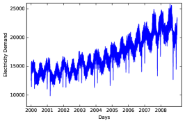
(a) Turkey electricity demand

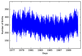
(b) Births in Quebec

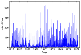
(c) Daily River Flows (Saugeen)

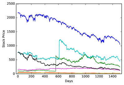
(d) Stock data

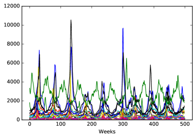
(e) Google flu data

Figure 3: Data plots. The top line has plots for univariate data, and the bottom line has plots for multivariate data.

References

- [1] Ili data set. http://www.cdc.gov/flu/weekly/overview.htm.
- [2] S&p data. https://finance.yahoo.com/quote/%5EGSPC/history/.
- Anava and Mannor [2016] Oren Anava and Shie Mannor. Heteroscedastic sequences: beyond gaussianity. In International Conference on Machine Learning, pages 755–763, 2016.
- Anava et al. [2013] Oren Anava, Elad Hzan, Shie Mannor, and Ohad Shamir. Online learning for time series prediction. In JMLR: Workshop and Conference Proceedings of Conference on Learning Theory, volume 13, 2013.
- Anava et al. [2015] Oren Anava, Elad Hazan, and Assaf Zeevi. Online time series prediction with missing data. In International Conference on Machine Learning, pages 2191–2199, 2015.
- Box et al. [2008] George Box, Gwilym Jenkins, and Gregory Reinsel. Time Series Analysis: Forecasting and Control. Wiley, 2008.
- Brockwell and Davis [2009] Peter Brockwell and Richard Davis. Time Series: Theory and Methods. Springer, 2009.
- Cesa-Bianchi and Lugosi [2006] Nicolo Cesa-Bianchi and Gábor Lugosi. Prediction, learning, and games. Cambridge university press, 2006.
- Duchi et al. [2008] John Duchi, Shai Shalev-Shwartz, Yoram Singer, and Tushar Chandra. Efficient projections onto the l 1-ball for learning in high dimensions. In Proceedings of the 25th international conference on Machine learning, pages 272–279. ACM, 2008.
- Elliot et al. [1996] Graham Elliot, Thomas J. Rothenberg, and James H. Stock. Efficient tests for an autoregressive unit root. Econometrica, 64:813–836, 1996.
- Hamilton [1994] James D Hamilton. Time series analysis princeton university press. Princeton, NJ, 1994.
- Hazan et al. [2007] Elad Hazan, Amit Agarwal, and Satyen Kale. Logarithmic regret algorithms for online convex optimization. Machine Learning, 69(2-3):169–192, 2007.
- Hazan et al. [2017] Elad Hazan, Karan Singh, and Cyril Zhang. Learning linear dynamical systems via spectral filtering. In Advances in Neural Information Processing Systems, pages 6705–6715, 2017.
- Johansen [1988] Soren Johansen. Statistical analysis of cointegration vectors. Journal of Economic Dynamics and Control, 12:1–47, 1988.
- Kuznetsov and Mohri [2016] Vitaly Kuznetsov and Mehryar Mohri. Time series prediction and online learning. In Proceedings of the Conference on Learning Theory, pages 1–24, 2016.
- Lai and Wei [1982] Tze Leung Lai and Ching Zong Wei. Least squares estimates in stochastic regression models with applications to identification and control of dynamic systems. The Annals of Statistics, pages 154–166, 1982.
- [17] Percy Liang. Cs229t/stat231: Statistical learning theory (winter 2014).
- Liu et al. [2016] Chenghao Liu, Steven CH Hoi, Peilin Zhao, and Jianling Sun. Online arima algorithms for time series prediction. In Thirtieth AAAI Conference on Artificial Intelligence, 2016.
- Ljung [1998] Lennart Ljung. System identification. In Signal Analysis and Prediction, pages 163–173. Springer, 1998.
- Lütkepohl [2005] Helmut Lütkepohl. New introduction to multiple time series analysis. Springer Science & Business Media, 2005.
- Lütkepohl [2006] Helmut Lütkepohl. Forecasting with varma models. Handbook of economic forecasting, 1:287–325, 2006.
- Shalev-Shwartz [2011] Shai Shalev-Shwartz. Online learning and online convex optimization. Foundations and Trends in Machine Learning, 4(2):107–194, 2011.
- Tsay [2013] Ruey Tsay. Multivariate Time Series Analysis: With R and Financial Applications. Wiley, 2013.
- Zinkevich [2003] Martin Zinkevich. Online convex programming and generalized infinitesimal gradient ascent. In ICML, 2003.