Symplectic neighborhood of crossing symplectic submanifolds

Abstract.

This paper presents a proof of the existence of standard symplectic coordinates near a set of smooth, orthogonally intersecting symplectic submanifolds. It is a generalization of the standard symplectic neighborhood theorem. Moreover, in the presence of a compact Lie group $G$ acting symplectically, the coordinates can be chosen to be $G$-equivariant.

Introduction

The main result in this paper is a generalization of the symplectic tubular neighborhood theorem (and the existence of Darboux coordinates) to a set of symplectic submanifolds that intersect each other orthogonally. This can help us understand singularities in symplectic submanifolds. Orthogonally intersecting symplectic submanifolds (or, more generally, positively intersecting symplectic submanifolds as described in the appendix) are the symplectic analogue of normal crossing divisors in algebraic geometry. Orthogonal intersecting submanifolds, as explained in this paper, have a standard symplectic neighborhood. Positively intersecting submanifolds, as explained in the appendix and in [TMZ14a], can be deformed to obtain the same type of standard symplectic neighborhood.

The result has at least two applications to current research: it yields some intuition for the construction of generalized symplectic sums (see [TMZ14b]), and it describes the symplectic geometry of degenerating families of Kähler manifolds as needed for mirror symmetry (see [GS08]). The application to toric degenerations is described in detail in the follow-up paper [Gua].

While the proofs are somewhat technical, the result is a natural generalization of Weinstein’s neighborhood theorem. Given a symplectic submanifold $X$ of $(M,\omega)$, there exists a tubular neighborhood embedding $\phi:NX\rightarrow M$ defined on a neighborhood of $X$. Moreover, an appropriate choice of connection $\alpha$ on $NX$ determines a closed 2-form $\omega_{\alpha}$, non-degenerate in a neighborhood of $X$ (see Section 2). Thanks to Weinstein’s symplectic neighborhood theorem [Wei71], the tubular neighborhood embedding can be chosen to be symplectic. The aim of the present work is to prove an analogous statement for a union of symplectic submanifolds $\{X_{i}\}_{i\in\mathcal{I}}$ of $(M,\omega)$. We require the intersection to be orthogonal, that is, $N(X_{i}\cap X_{j})=NX_{i}\oplus^{\perp}NX_{j}$, for all $i,j$, at all intersection points (see Definition 3).

Remark.

The generalization from one to multiple submanifolds is not straightforward, because there is no smooth retraction of a neighborhood of $\bigcup_{i\in\mathcal{I}}X_{i}$ onto $\bigcup_{i\in\mathcal{I}}X_{i}$ when $|\mathcal{I}|>1$. The goal of this paper is to overcome such difficulty.

The result can be summarized as follows (see Corollary 6.1, and see Theorem 7.6 for the equivariance):

Theorem 1.

Let $\{X_{i}\}_{i\in\mathcal{I}}$ be a finite family of orthogonal symplectic submanifolds in $(M,\omega)$. Then there exist connections $\alpha_{i}$ on $NX_{i}$ and symplectic neighborhood embeddings $\phi_{i}:(NX_{i},\omega_{\alpha_{i}})\rightarrow(M,\omega)$ which are pairwise compatible.

In the presence of a group $G$, the embeddings can be chosen to be equivariant with respect to the linearized action.

If we assume that the manifolds are of real codimension $2$ (e.g. algebraic divisors), compatibility can be expressed as follows: for all $i,j$, for $X_{ij}=X_{i}\cap X_{j}$, there is a symplectic neighborhood embedding $\phi_{ij}:(NX_{ij},\omega_{\alpha_{i}+\alpha_{j}})\rightarrow(M,\omega)$, which factors as $\phi_{ij}=\phi_{i}\circ\xi_{ij}^{i}=\phi_{j}\circ\xi_{ij}^{j}$, where $\xi_{ij}^{i}:NX_{ij}\cong(NX_{i}\oplus NX_{j})|_{X_{ij}}\rightarrow NX_{i}$ is a morphism of symplectic vector bundles covering some symplectic neighborhood map $\varphi_{ij}^{i}:N_{X_{i}}X_{ij}\rightarrow X_{i}$ (and similarly for $j$) while $\phi_{i},\phi_{j}$ are symplectic tubular neighborhood maps.

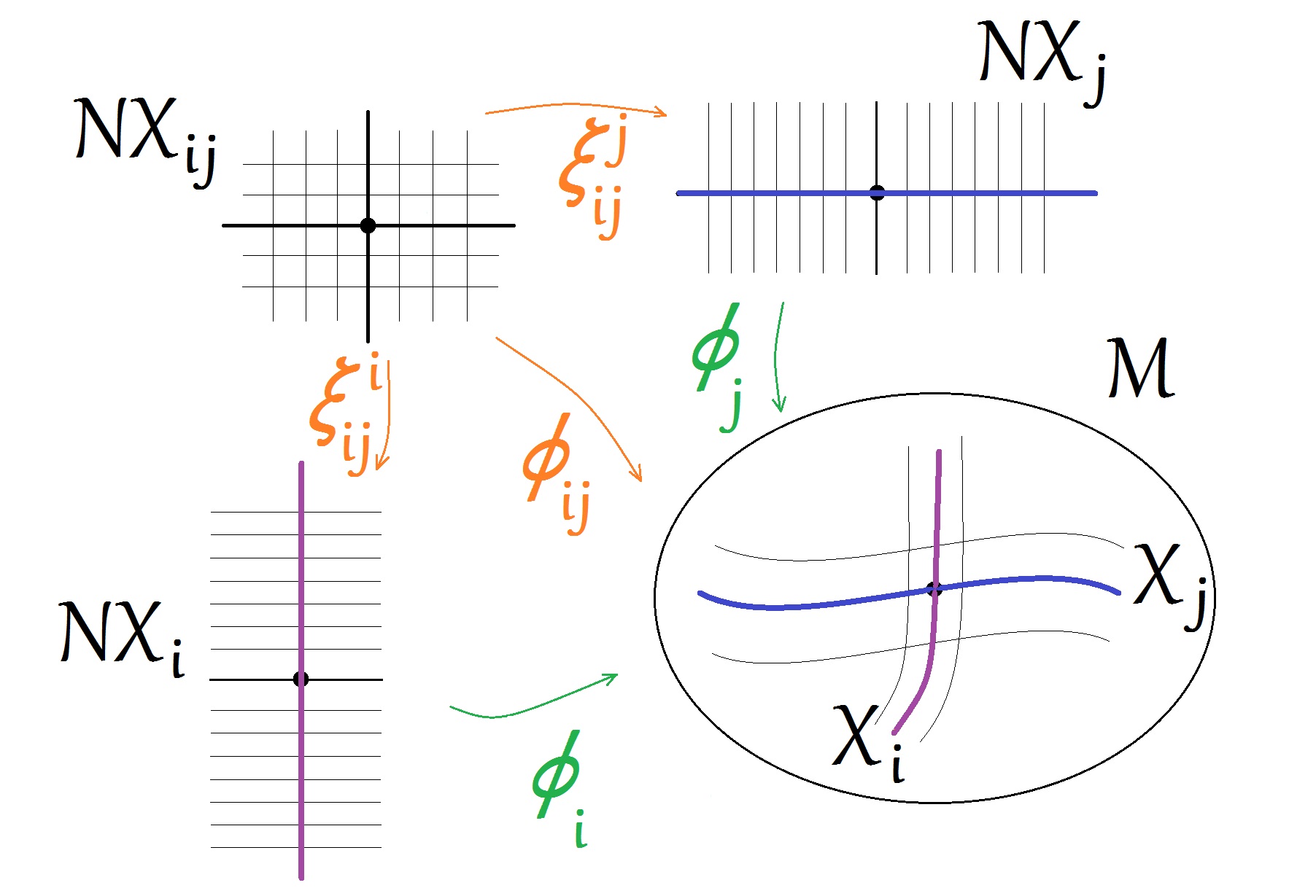
Figure 1. The compatibility of $\phi_{i},\phi_{j}$ is given by the existence of $\phi_{ij},\xi_{ij}^{i},\xi_{ij}^{j}$.

The result (and the more general compatibility conditions) can be expressed in terms of the auxiliary construction of a symplectic plumbing. A plumbing is an appropriate gluing of the normal bundles $NX_{i}$ for all $i$, and if we keep track of some extra data we can make sure it inherits a symplectic form. The content of Theorem 6.2 and Theorem 7.6 can be summarized as follows:

Theorem 2 (reformulation of Theorem 1).

Given a family of orthogonally intersecting submanifolds $\{X_{i}\}_{i\in\mathcal{I}}$ in $(M,\omega)$, there exists a symplectic space given by a union of all the normal bundles, called plumbing. The union $\bigcup_{i}X_{i}$ admits a neighborhood in $M$ which is symplectomorphic to a neighborhood of the zero section in the plumbing.

In the presence of a $G$-action, the plumbing inherits a linearized $G$-action and the symplectomorphism can be chosen to be equivariant.

This implies Theorem 1.

Outline of proof. For symplectic submanifolds $\{X_{i}\}_{i\in\mathcal{I}}$, $X_{i}\subset(M,\omega)$, the symplectic form $\omega$ on a neighborhood of $\bigcup_{i}X_{i}$ only depends on the restriction of $\omega$ to ${TM|_{\bigcup_{i}X_{i}}}$. This is the content of Lemma 1. It is a generalization of the case of one divisor, and it is done by induction.

The rest of the paper gives an explicit construction of a local model for such a symplectic form. This is done in Theorem 6.2. The strategy is to first construct an appropriate space containing $\bigcup_{i}X_{i}$, which is diffeomorphic to a neighborhood of $\bigcup_{i}X_{i}$ in $M$. This can be done by constructing a plumbing, that is, an appropriate glueing of the normal bundles $NX_{i}$ for all $i$. Unfortunately, the construction doesn’t run as smoothly when introducing symplectic structures. Therefore, we give a definition of plumbing which is more rigid than usual and requires some extra data (see Definition 4). This set of rigid data is needed in order to use the result in symplectic settings. The fact that such data always exist is proved in Theorem 5.2. We then show that if a plumbing is built symplectically (as in Definition 8), then it admits a symplectic form, which only depends on the symplectic bundle structure of each $NX_{i}$, together with a choice of compatible connections for each $NX_{i}$. This is the content of Lemma 14. The fact that one can always find connections which have the right compatibility is proved in Lemma 13.

The main theorem (Theorem 6.2) states that a symplectic plumbing can be constructed for any choice of orthogonal symplectic submanifolds, and it can always be symplectically embedded as a neighborhood of such submanifolds in $M$. The proof follows the outline of the proof of the symplectic neighborhood theorem: first, construct a smooth embedding of the plumbing (see Proposition 5.2), whose derivative is the identity along each $X_{i}$; then, apply Lemma 1 to make it a symplectomorphism. The case of multiple submanifolds requires more care than the classical case, due to the compatibility requirements (the main problem is: there isn’t a smooth retraction onto $\bigcup_{i}X_{i}$; so we need to use separate retractions onto $X_{i}$ for each $i$, and insure compatibility at every step).

The last section of the paper extends the results in the presence of a compact Lie group acting symplectically. When such $G$ acts on $(M,\omega)$ and preserves each submanifold $X_{i}$, we construct a $G$-action on the plumbing (given by linearizing the action on each $NX_{i}$). This is done in Lemma 7.4. Finally, in Theorem 7.6, we show that, if $G$ acts symplectically on $M$, the right choice of connections makes the plumbing a symplectic $G$-space, and the symplectic embedding of the plumbing into $M$ can be chosen to be equivariant.

Acknowledgments. Many thanks to Mark McLean and Mohammad Tehrani for helpful conversation, and to Tim Perutz for his advice and patience. This work was partly supported by the NSF through grants DMS-1406418 and CAREER-1455265.

1. Symplectic forms on neighborhoods of crossing symplectic submanifolds

Let $\omega_{1},\omega_{2}$ be symplectic forms on $M$. Let $\{X_{i}\}_{i\in I}$ be a collection of symplectic submanifolds of both $(M,\omega_{1})$ and $(M,\omega_{2})$. Throughout the paper we’ll assume that all intersections are transverse. What follows is a version of Moser’s argument for symplectic forms agreeing on transversal symplectic submanifolds.

Definition 1.

Two forms $\alpha,\beta$ on $M$ are said to agree along a subset $S\subseteq M$ whenever $\alpha_{x}=\beta_{x}$ on $T_{x}M$ for all $x\in S$.

Lemma 1.

Assume that $\omega_{1}$, $\omega_{2}$ are symplectic forms on $M$ that agree along $\bigcup_{i}X_{i}$. Then there exist open neighborhoods $\mathcal{U},\mathcal{V}$ of $\bigcup_{i}X_{i}$ and a diffeomorphism $\phi:\mathcal{U}\rightarrow\mathcal{V}$ such that

$$\phi|_{\bigcup_{i}X_{i}}=id\;\ \ \ \ \ \ \ \phi^{*}\omega_{2}=\omega_{1}.$$

Proof.

We will approach the proof by induction: for all $0\leq k\leq n$ we’ll find:

• a 2-form $\omega^{(k)}$ such that $\omega^{(k)}=\omega_{1}=\omega_{2}$ along all $X_{i}$’s, $\omega^{(k)}=\omega_{1}$ in a neighborhood of $\bigcup_{i=1}^{k}X_{i}$;

• $f_{k}$ such that $f_{k}^{*}(\omega^{(k-1)})=\omega^{(k)}$, $f_{k}=id$ on $X_{i}$ for all $i$, and $f_{k}=id$ on a neighborhood of $\bigcup_{i=1}^{k-1}X_{i}$.

The starting point will be $\omega^{(0)}=\omega_{2}$, and at the end $\phi=f_{1}\circ\ldots\circ f_{n}$ will satisfy $\phi^{*}\omega_{2}=\omega^{(n)}=\omega_{1}$.

Assume, for $k>0$, that $\omega^{(k-1)}$ has been built. To construct $f_{k}$, we’ll find a 1-form $\sigma_{k}$ such that $d\sigma_{k}=\omega^{(k-1)}-\omega_{1}$ on a neighborhood of $X_{k}$, $\sigma_{k}=0$ along all $X_{i}$’s and $\sigma_{k}=0$ on a neighborhood of $\bigcup_{i=1}^{k-1}X_{k}$; Moser’s theorem applied to $\sigma_{k}$ yields $f_{k}:\mathcal{U}_{k}\rightarrow\mathcal{V}_{k}$ and $\omega^{(k)}=f_{k}^{*}(\omega^{(k-1)})$ as desired.

To construct $\sigma_{k}$, consider the exponential map with respect to a metric $g$, and let $exp_{k}:N_{M}X_{k}\cong T_{X_{k}}M^{\perp_{g}}\rightarrow M$ be the restriction of this map to the normal bundle of $X_{k}$ (Really, we are only considering this map for vectors of length at most $\delta$ so that $exp_{k}$ is a diffeomorphism. The slight abuse of notation reflects an effort to keep the notation from getting too heavy). Let $\mathcal{N}_{k}$ be the image of such map, i.e. a tubular neighborhood of $X_{k}$. We make sure to pick $g$ such that $exp_{k}$ restricts to a map $exp_{k}|_{N_{X_{j}}(X_{k}\cap X_{j})}:{N_{X_{j}}(X_{k}\cap X_{j})}\rightarrow X_{j}$ for all $j\neq k$ (we’ll construct such a metric later in this paper; see Corollary 4.1). Now define $\phi_{t}:\mathcal{N}_{k}\rightarrow\mathcal{N}_{k}$, the map sending $exp_{k}(q,v)\mapsto exp_{k}(q,tv)$. In particular, for all $j\neq k$, $\phi_{t}$ restricts to a map from $X_{j}\cap\mathcal{N}_{k}$ to itself.

(Notation reminder: when $(q,v)\in T^{vert}_{q}(M)$, $m\in M$, $exp(q,v)\in M$, then $\omega(m;v,w)$ denotes $\omega$ at the point $m$ evaluated on $v,w\in T_{m}(M)$; similarly for a one form $\sigma(m;v)$ denotes $\sigma$ at the point $m$ evaluated on $v$.)

Now we want to consider the family of one-forms on $M$:

$$\sigma_{t}(m;v)=(\omega^{(k-1)}-\omega_{1})(\phi_{t}(m);\frac{d}{dt}\phi_{t}(m),d\phi_{t}(m)v)$$

and integrate it to get

$$\tilde{\sigma}_{k}(m)=\int_{0}^{1}\sigma_{t}(m)$$

If $m\in X_{j}$, then $\phi_{t}(m)\in X_{j}$ (due to the choice of metric). Because $(\omega^{(k-1)}-\omega_{1})$ vanishes on $X_{j}$, $\sigma_{t}(m;v)=0$ for all $v$. Therefore $\tilde{\sigma}_{k}(m)=\int_{0}^{1}\sigma_{t}(m)=0$. Now we can extend $\tilde{\sigma}_{k}$ to a full neighborhood of $\bigcup_{i}X_{i}$ by letting $B_{\epsilon}(X_{k})\subset\mathcal{N}$ be a smaller neighborhood of $X_{k}$, and define

$$\sigma_{k}=\begin{cases}\hfill\tilde{\sigma}_{k}\hfill&\text{ if }x\in B_{\epsilon}(X_{k})\\ \hfill 0\hfill&\text{ if }x\notin\mathcal{N}\\ \hfill\text{}\hfill&\text{smoothly interpolates on }\mathcal{N}\backslash B_{\epsilon}\\ \end{cases}$$

Such $\sigma_{k}$ is as required and yields a diffeomorphism $f_{k}:\mathcal{U}_{k}\rightarrow\mathcal{V}_{k}$. Also notice that $f_{k}=id$ whenever $\sigma_{k}=0$, in particular on $\bigcup_{i}X_{i}$ and on a neighborhood of $\bigcup_{i=1}^{k-1}X_{i}$. Let then $\omega^{(k)}=f_{k}^{*}\omega^{(k-1)}$: by construction, $\omega^{(k)}=\omega_{1}=\omega_{2}$ along all $X_{i}$’s, $\omega^{(k)}=\omega_{1}$ in a neighborhood of $\bigcup_{i=1}^{k}X_{i}$.

∎

Remark.

1. The transversality condition can be somewhat relaxed and the proof of the lemma still works in some cases, think e.g. two lower dimensional submanifolds that are not tangent at the intersection points. Weaker formulations can be found if needed.

2. This lemma doesn’t need orthogonality for the intersection of the $X_{i}$’s.

3. The lemma can be easily modified to include self-crossing submanifolds.

4. It is tempting to avoid induction and look for a proof by first constructing a retraction of a neighborhood of $\bigcup_{i}X_{i}$ onto $\bigcup_{i}X_{i}$, then using Moser’s argument only once on the resulting vector field; however, this argument wouldn’t work because such a retraction is not smooth; hence the need for induction.

In order to use Lemma 1 to prove the existence of a nice neighborhood of intersecting submanifolds $\{X_{i}\}_{i\in\mathcal{I}}$, we need to find a multifold analogue of the following classical theorem, which is used in the classic result of Weinstein [Wei71] (for a detailed discussion of Weinstein’s result cfr. [MS98]):

Theorem (Tubular neighborhood theorem).

There exists a map from $NX$ to $M$ such that $f|_{X}=id$ and $df|_{X}=id$.

Classically, such a map can be obtained as the exponential map of any metric, applied to $T^{\perp_{\omega}}_{X}M$ (which is naturally isomorphic to $NX$). This can be much harder to prove (or even state) for $X$ not smooth.

2. Normal bundles and connections

This section is a review of some basic facts for complex and symplectic vector bundles.

Remarks on notation. For submanifolds $Z\subset X\subset M$, $N_{M}X$ will indicate the normal bundle to $X$ inside $M$ (sometimes only $NX$ when there is no ambiguity), so that $N_{X}Z$ is the normal bundle to $Z$ inside $X$, while $NX|_{Z}$ indicates the restriction to $Z$ of the normal bundle to $X$ inside $M$.

The normal bundle to a symplectic submanifold is naturally a symplectic bundle. Recall that one can always choose a compatible complex structure on a symplectic bundle: the choice is unique up to isotopy. Moreover, two bundles are isomorphic as symplectic bundles if and only if they are isomorphic as complex bundles (see e.g. [MS98]). Therefore we will chose complex structures and consider the normal bundles as complex bundles.

There will be some abuse of notation with respect to connections on normal bundles: given $Y\subset X$ a symplectic submanifold of real codimension $2$, one can obtain a model for the complex normal bundle by letting $NY=U\times_{U(1)}\mathbb{C}$ where $U$ is a principal $U(1)$-bundle and $\alpha$ is a $U(1)$-connection on $U$. Whenever the paper mentions a connection $\alpha$ on $NX$, it can be interchangeably a connection 1-form on a $U(1)$-bundle (for which $NX$ is the associated bundle) or the corresponding Ehresmann connection on $NX$.

Remark.

Choosing a $U(1)$-connection $\alpha$ gives the same data as a unitary Ehresmann connection on $NX$, whence the abuse of notation.

One can then build a two-form on $U\times\mathbb{C}$:

$$\omega_{\alpha}=\omega_{Y}+d(\rho\alpha)+\omega_{\mathbb{C}}$$

where $\rho$ indicates the hamiltonian function generating the standard circle action on $\mathbb{C}$. Such two-form descends to $U\times_{U(1)}\mathbb{C}$. This is a general fact:

Lemma 2.

Let $(F,\omega_{F})$ be a symplectic manifold, $G\circlearrowright F$ a Hamiltonian action with moment map $\mu$, $P$ a principal $G$-bundle over a symplectic base $(Y,\omega_{Y})$, $X=P\times_{G}F$ the associated bundle, $\alpha$ a principal connection on $P$. Then the 2-form $\omega_{F}+d\langle\alpha,\mu\rangle$ on $P\times F$ descends to a $2-form$ on $X$. Therefore so does $\Omega=\omega_{Y}+d\langle\alpha,\mu\rangle+\omega_{F}$ (here $\omega_{Y}$ is short for $\pi^{*}(\omega_{Y})$).

Proof.

Let $v_{\xi}$ be the vector field on $P\times F$ corresponding to $\xi\in\mathfrak{g}$. Recall that a form $\eta$ on $P\times F$ is the pullback of a form on $X$ if and only if $\iota_{v_{\xi}}\eta=\mathcal{L}_{v_{\xi}}\eta=0$, which by Cartan’s formula is equivalent to $\iota_{v_{\xi}}\eta=\iota_{v_{\xi}}(d\eta)=0$. Since $\omega_{F}+d\langle\alpha,\mu\rangle$ is closed we will just check that, for every $\xi\in\mathfrak{g}$, $\iota_{v_{\xi}}(\omega_{F}+d\langle\alpha,\mu\rangle)=0$.

Since $\mathcal{L}_{v_{\xi}}\alpha=0$, also $\mathcal{L}_{v_{\xi}}(d\langle\alpha,\mu\rangle)=0$ therefore

$$\iota_{v_{\xi}}\circ d\langle\alpha,\mu\rangle=\iota_{v_{\xi}}<d\alpha,\mu>-\iota_{v_{\xi}}(\alpha\wedge d\mu)\text{ by expanding the derivative}$$

$$=-\iota_{v_{\xi}}(\alpha\wedge d\mu)\text{ because the other term is 0 when $\alpha$ is a principal connection}$$

$$=-<\xi,d\mu>=-d<\xi,\mu>=\iota_{\xi_{P}}\omega_{F}$$

so that $\iota_{v_{\xi}}(\omega_{F}+d\langle\alpha,\mu\rangle)=\iota_{\xi_{P}}\omega_{F}-\iota_{\xi_{P}}\omega_{F}=0$. ∎

We can also find a more explicit description of $\Omega$ on $X$. First note that the tangent bundle of $P$ splits as $T^{vert}P\oplus T^{hor}P$. Let $\pi:P\rightarrow Y$ be the projection, then the horizontal component $T^{hor}P:=\ker\alpha$ is identified by $D\pi$ with $\pi^{*}TY$, while the vertical component is $T^{vert}P:=\ker D\pi=\mathfrak{g}$. Thus (omitting notation for pullbacks of projections) we have $T(P\times F)=\mathfrak{g}\oplus\pi^{*}TY\oplus TF$, and $\mathfrak{g}$ acts on $T(P\times F)$ by $\xi\mapsto(-\xi,0,\xi_{F})$, hence

$$TX\cong\pi^{*}TY\oplus TF.$$

In other words, a tangent vector $z\in TX$ may be uniquely rewritten as $z=u^{\natural}+v$, where $u^{\natural}$ is the horizontal lift of $u\in TY$ to $TP$ while $v\in TF$. Moreover, the vector $\tilde{z}=(0,u^{\natural},v)\in\mathfrak{g}\oplus\pi^{*}TY\oplus TF\cong T(P\times F)$ projects to $z$. This means that one can compute $\Omega(z_{1},z_{2})$ by evaluating $\Omega(\tilde{z}_{1},\tilde{z}_{2})$.

Now let’s describe $\Omega$. First recall that the curvature is $F_{\alpha}\in\Omega^{2}(M;P\times_{G}\mathfrak{g})$. It induces a 2-form via pullback on $P$: $\pi^{*}F_{\alpha}=d\alpha+\frac{1}{2}[\alpha\wedge\alpha].$ Notice that $d\langle\alpha,\mu\rangle=\langle d\alpha,\mu\rangle+\langle\alpha\wedge d\mu\rangle$ on $P\times F$; the key observation is that $\alpha(\tilde{z}_{1})=\alpha(\tilde{z}_{2})=0$. Then we can calculate

$$\Omega(z_{1},z_{2})=\Omega(\tilde{z}_{1},\tilde{z}_{2})=$$

$$=\omega_{Y}(u_{1},u_{2})+\langle d\alpha(\tilde{z}_{1},\tilde{z}_{2}),\mu\rangle+\frac{1}{2}(\langle\alpha(\tilde{z}_{1}),d\mu(\tilde{z}_{2})\rangle-\langle\alpha(\tilde{z}_{2}),d\mu(\tilde{z}_{1})\rangle)+\omega_{F}(v_{1},v_{2})$$

$$=\omega_{Y}(u_{1},u_{2})+\langle d\alpha(\tilde{z}_{1},\tilde{z}_{2}),\mu\rangle+\omega_{F}(v_{1},v_{2})$$

$$=\omega_{Y}(u_{1},u_{2})+\langle(\pi^{*}F_{\alpha}-\frac{1}{2}[\alpha\wedge\alpha])(\tilde{z}_{1},\tilde{z}_{2}),\mu\rangle+\omega_{F}(v_{1},v_{2})$$

$$=\omega_{Y}(u_{1},u_{2})+\langle\pi^{*}F_{\alpha}(\tilde{z}_{1},\tilde{z}_{2}),\mu\rangle-\langle\frac{1}{2}[\alpha\wedge\alpha])(\tilde{z}_{1},\tilde{z}_{2}),\mu\rangle+\omega_{F}(v_{1},v_{2})$$

$$=\omega_{Y}(u_{1},u_{2})+\langle F_{\alpha}(u_{1},u_{2}),\mu\rangle+\omega_{F}(v_{1},v_{2}).$$

Example 2.1.

If, for instance, $\alpha$ is the flat connection induced by a trivialization, then the form on $Y\times F$ is given by $\omega_{Y}+\omega_{F}$. In fact this is an if and only if. In slightly different words: $F_{\alpha}$ is the obstruction to $\omega_{F}$ pushing forward to a form on $X$.

Corollary 2.1.

For a complex line bundle $U\times_{U(1)}\mathbb{C}$, with a connection $\alpha$, over a symplectic base $(Y,\omega_{Y})$ the 2-form $\omega_{\alpha}=\omega_{Y}+d(\rho\alpha)+\omega_{\mathbb{C}}$ descends to a closed 2-form on $U\times_{U(1)}\mathbb{C}$. This form can be described as $\omega_{Y}+\rho F_{\alpha}+\omega_{\mathbb{C}}$ with respect to a horizontal/vertical splitting due to $\alpha$.

Similarly, if $Y\subset M$ has codimension $2k$ and $NY=\bigoplus_{s=1}^{k}\mathcal{L}_{s}$ is a sum of line bundles, then $NY=U\times_{U(1)^{k}}\mathbb{C}^{k}$ where $U$ is the sum of unit bundles inside $L_{s}$’s. If $\alpha_{s}$’s are $U(1)$-connections, then $\bigoplus_{s=1}^{k}\alpha_{s}$ is a connection on $U$ and the induced symplectic form on a tubular neighborhood of $Y$ is

$$\omega_{\oplus_{s}\alpha_{s}}=\omega_{Y}+\sum_{s}(\rho_{s}F_{\alpha_{s}})+\omega_{\mathbb{C}^{k}}.$$

Corollary 2.2.

Let’s consider the case of $Y\subset M$ of (real) codimension higher than two. Then $NY$ is a $\mathbb{C}^{k}$-bundle and the structure group is $G=U(k)$. Given a connection form $\alpha$ on the corresponding principal $G$ bundle $P$, we get an induced symplectic form

$$\omega_{\alpha}=\omega_{Y}+\langle F_{\alpha},\mu\rangle+\omega_{\mathbb{C}^{k}}.$$

More in general we can define $\omega_{\oplus_{s}\alpha_{s}}$ on a sum of bundles, where $\alpha_{s}$ is the connection on a complex vector bundle of dimension $k_{s}$ over $Y$:

$$\omega_{\oplus_{s}\alpha_{s}}=\omega_{Y}+\sum_{s}\langle F_{\alpha_{s}},\mu_{s}\rangle+\omega_{\mathbb{C}^{\sum_{s}k_{s}}}.$$

3. A remark on transversality

In the rest of the discussion all collections of submanifolds will be transverse in the following sense:

Definition 2.

Let $\{X_{i}\}_{i\in\mathcal{I}}$ be a finite collection of submanifolds of $M$. Let $X_{I}=\bigcap_{i\in I}X_{i}$ for all subsets $I\subseteq\mathcal{I}$. The collection is called transverse if $NX_{I}=\oplus_{i\in I}NX_{i}|_{X_{I}}$.

This is stronger than just pairwise transversality. On the other hand, once we move to the symplectic world, we assume orthogonality in the following sense:

Definition 3.

The intersection of two symplectic submanifolds $X_{1},X_{2}\subset(M,\omega)$ is orthogonal if there is an orthogonal decomposition $TM=TX_{12}\oplus^{\perp}NX_{1}\oplus^{\perp}NX_{2}$.

Remark.

This definition in particular implies that the two submanifolds are transverse. If you care about other situations (e.g. two Riemann surfaces intersecting in $\mathbb{R}^{6}$ with linearly independent tangent spaces) then you should look for slightly different definitions. The results in this paper can be adapted to other reasonable definitions.

For a family of orthogonal intersection, we can afford to only make pairwise assumptions, because of the following:

Lemma 3.

Let $\{X_{i}\}_{i\in\mathcal{I}}$ be a finite collection of symplectic submanifolds of $(M,\omega)$. Assume that, whenever $i\neq j$, $X_{i},X_{j}$ intersect orthogonally. Then $\{X_{i}\}_{i\in\mathcal{I}}$ is a transverse collection.

Proof.

The key observation is that for orthogonal sums, $NX_{i}\perp NX_{j}$ for all $j\neq i$ implies $NX_{i}\perp\oplus_{j\in J}NX_{j}$ whenever $i\notin J$. This means $\{NX_{i}\}_{i\in I}$ is a linearly independent collection of subspaces in $TM$. Pick a point $x\in X_{I}$. Notice that there is an embedding $N_{x}X_{i}\overset{\iota_{i}}{\hookrightarrow}N_{x}X_{I}$ when $i\in I$ (if a vector is orthogonal to $X_{i}$ then it must also be orthogonal to the subset $X_{I}$). Now let’s consider the map $\oplus_{i}\iota_{i}:\oplus_{i\in I}N_{x}X_{i}\rightarrow NX_{I}$. This map is injective since $NX_{i}\subset NX_{I}$ are linearly independent subspaces. It is then an isomorphism because of dimensions. We can use the formula for the dimension of an intersection of vector subspaces and get $\dim(T_{x}X_{I})=\dim(\bigcap_{i\in I}T_{x}X_{i})\geq\sum_{i}\dim TX_{i}-(k-1)\cdot n=\sum_{i\in I}(n-\dim NX_{i})-(k-1)\cdot n=n-\sum_{i\in I}\dim NX_{i}$ (here $k=\#I$, $n=\dim(TM)$. Then $\dim NX_{I}=n-\dim(T_{x}X_{I})\leq n-(n-\sum_{i\in I}\dim(NX_{i}))=\sum_{i\in I}\dim NX_{i}$. ∎

4. Plumbing for smooth manifolds

This section is devoted to carefully describing smooth plumbings and their embedding. The plumbings that we will consider later are enhanced versions of the smooth ones.

Remark on notation: Throughout the paper, for each $I\subset\mathcal{I}$, $X_{I}:=\bigcap_{i\in I}X_{i}$ will denote the intersection.

4.1. Plumbing data

Let $\{X_{i}\}_{i\in\mathcal{I}}$ be a finite collection of smooth submanifolds in $M$. Let their intersections be transverse (as in Definition 2).

In order to build and embed a plumbing, we need the following:

Definition 4.

A system of tubular neighborhoods for the family $\{X_{i}\}_{i\in\mathcal{I}}$ is a collection of tubular neighborhood maps

$$\psi_{I}^{I^{\prime}}:N_{X_{I^{\prime}}}X_{I}\rightarrow X_{I^{\prime}}\text{\ \ \ \ \ \ \ }\forall I^{\prime}\subset I\subset\mathcal{I}\text{\ \ \ \ \ \ \ \ }I^{\prime}\neq\emptyset$$

where the maps are defined on a neighborhood $\mathcal{V}_{I}^{I^{\prime}}$ of $X_{I}$ in $N_{X_{I^{\prime}}}X_{I}$. We require that the restriction of $\psi_{I}^{I^{\prime}}$ to $X_{I}$ is the identity. Let $\mathcal{U}_{I}^{I^{\prime}}=Im(\mathcal{V}_{I}^{I^{\prime}})$ be the corresponding neighborhood in $X_{I^{\prime}}$. The maps naturally induce smooth retractions $\rho_{I}^{I^{\prime}}=\pi\circ(\psi_{I}^{I^{\prime}})^{-1}:\mathcal{U}_{I}^{I^{\prime}}\rightarrow X_{I}$.

We require that $\rho_{I}^{I^{\prime}}\circ\rho_{I^{\prime}}^{I^{\prime\prime}}=\rho_{I}^{I^{\prime\prime}}:U_{I}^{I^{\prime\prime}}\rightarrow X_{I}$ for all $I^{\prime\prime}\subset I^{\prime}\subset I$.

A system of bundle isomorphisms covering the retractions is a collection of maps $\Phi_{I}^{I^{\prime}}:NX_{I}\rightarrow NX_{I^{\prime}}|_{\mathcal{U}_{I}^{I^{\prime}}}$ given by a choice of isomorphisms $\widetilde{\Phi}_{I}^{I^{\prime}}:(\rho_{I}^{I^{\prime}})^{*}(NX_{I^{\prime}}|_{X_{I}})\rightarrow NX_{I^{\prime}}|_{\mathcal{U}_{I}^{I^{\prime}}}$. The maps are defined as

$$\Phi_{I}^{I^{\prime}}=\widetilde{\Phi}_{I}^{I^{\prime}}\circ(\psi_{I}^{I^{\prime}},id):NX_{I}\cong N_{X_{I^{\prime}}}X_{I}\oplus NX_{I^{\prime}}|_{X_{I}}\rightarrow NX_{I^{\prime}}|_{\mathcal{U}_{I}^{I^{\prime}}}.$$

The data of a system of tubular neighborhoods together with a system of bundle isomorphisms is compatible when, for all $I^{\prime\prime}\subset I^{\prime}\subset I$:

• $\psi_{I}^{I^{\prime\prime}}=\psi_{I^{\prime}}^{I^{\prime\prime}}\circ(\Phi_{I}^{I^{\prime}})|_{X_{I^{\prime\prime}}}:N_{X_{I^{\prime\prime}}}X_{I}\rightarrow N_{X_{I^{\prime\prime}}}X_{I^{\prime}}|_{\mathcal{U}_{I}^{I^{\prime}}}\rightarrow X_{I^{\prime\prime}};$

• $\Phi_{I}^{I^{\prime\prime}}=\Phi_{I^{\prime}}^{I^{\prime\prime}}\circ\Phi_{I}^{I^{\prime}}:NX_{I}\rightarrow NX_{I^{\prime\prime}}.$

We also refer to this set of compatible data as plumbing data.

Given the data above, we can define smooth plumbings:

Definition 5.

Given a finite family of smooth submanifold $\{X_{i}\}_{i\in\mathcal{I}}$ where $|\mathcal{I}|=n$; given a system of tubular neighborhoods and a system of bundle isomorphisms that are compatible, the (n)-plumbing of the family is

$$N(\bigcup_{i}X_{i})=\bigcup_{i}NX_{i}/\sim$$

where $\sim$ is the equivalence relation given by $\Phi_{I}^{i}(x)\sim\Phi_{I}^{j}(x)$ for all $I$, for all $i,j\in I$. The (n)-plumbing will be referred to as plumbing when there is no ambiguity.

Let’s check that this is a good definition (nothing bad happens at higher intersections):

Lemma 4.

The inclusion $NX_{i}\hookrightarrow\bigcup_{i}NX_{i}/\sim$ is injective. Therefore, the plumbing is a smooth manifold.

Proof.

We need to show that each point of $NX_{i}$ in a neighborhood of $X_{ij}$ is identified with exactly one point of $NX_{j}$. The trouble potentially arises at higher intersection points. Consider a neighborhood of $X_{ijk}$. Consider a point $(z,v_{i},v_{j},v_{k})\in NX_{ijk}\cong NX_{i}\oplus NX_{j}\oplus NX_{k}$. When looking at the equivalence relation from $NX_{i}$ to $NX_{j}$ we get

$$N(X_{i})\ni\Phi_{ij}^{i}(\Phi_{ijk}^{ij}(z,v_{k},v_{j},v_{i}))\sim\Phi_{ij}^{j}(\Phi_{ijk}^{ij}(z,v_{k},v_{j},v_{i}))\in N(X_{j}).$$

On the other hand if we consider $NX_{j}$ and $NX_{k}$ we get

$$N(X_{j})\ni\Phi_{jk}^{j}(\Phi_{ijk}^{jk}(z,v_{k},v_{j},v_{i}))\sim\Phi_{jk}^{k}(\Phi_{ijk}^{jk}(z,v_{k},v_{j},v_{i}))\in N(X_{k})$$

while $NX_{i},NX_{k}$ yield

$$N(X_{i})\ni\Phi_{ik}^{i}(\Phi_{ijk}^{ik}(z,v_{k},v_{j},v_{i}))\sim\Phi_{ik}^{k}(\Phi_{ijk}^{ik}(z,v_{k},v_{j},v_{i}))\in N(X_{k})$$

so $NX_{i}$ gets identified with $NX_{k}$ both directly and through $NX_{j}$: do the two identifications agree? We can use the compatibility assumption, $\Phi_{I^{\prime}}^{I^{\prime\prime}}\circ\Phi_{I}^{I^{\prime}}=\Phi_{I}^{I^{\prime\prime}}$. All the above relations then reduce to

$$(\Phi_{ijk}^{i}(z,v_{k},v_{j},v_{i}))\sim(\Phi_{ijk}^{j}(z,v_{k},v_{i},v_{j}))\sim(\Phi_{ijk}^{k}(z,v_{i},v_{j},v_{k})).$$

∎

Remark (Important).

The data used to construct the (n)-plumbing consists of a set of maps which can be thought of as the data of, for each $X_{i}$, the (n-1)-plumbing of its intersection with the other submanifolds, plus an embedding of such (n-1)-plumbing into $X_{i}$.

4.2. Metrics on plumbings

Lemma 5.

Given a smooth submanifold $X\subset M$, one can construct metrics on $NX$ which make $X$ totally geodesic, make the fibres $N_{x}X$ totally geodesic (for all $x\in X$), and are linear on the fibres $N_{x}X$ (when there is no ambiguity, we will call this type of metric a bundle metric on $NX$).

Proof.

We can freely choose the following data:

• A metric $g$ on X;

• A smoothly varying family of linear metrics $g_{x}$ on the fibres, that is, a bundle metric (it can be easily constructed locally, and local patches can be used to construct a global bundle metric through a partition of unity);

• A metric connection on $NX$ (this is equivalent to a choice of principal connection on the bundle of orthonormal frames).

Now let’s define the metric $\lambda$ on $NX$, on a local trivialization of $NX$, as $\lambda=g+g_{x}$ (with respect to the Ehresmann splitting $T_{p}(NX)\cong T_{x}X\oplus N_{x}X$). We can observe that such local definitions agree on chart intersections and form a metric on the whole bundle.

It is clear then that $\lambda$ makes $X$ and $N_{x}X$ totally geodesic, because this property can be checked locally. Locally, the bundle looks like $(\mathcal{U}\times N_{x}X,g+g_{x})$, where $\mathcal{U}$ is an open set in $X$; with respect to the local trivialization, $g_{x}$ is independent of $x$. ∎

The following lemma is the key to constructing well behaved metrics on plumbings.

Lemma 6.

Given a plumbing, assume that there is a metric $g$ on $\bigcup_{i}X_{i}$ (that is, metrics $g_{i}$ defined on each $X_{i}$, agreeing on intersections) such that $\psi_{I}^{J}=exp_{g}:N_{X_{J}}X_{I}\rightarrow X_{J}$ for all non-empty $J\subset I\subseteq\mathcal{I}$. Moreover let’s assume that $(\psi_{ij}^{i})^{*}g_{i}=\lambda_{j}$ on $N_{X_{i}}X_{ij}\cong NX_{j}|_{X_{ij}}$ is a bundle metric as in Lemma 5 (in particular it is linear in the fibres of $N_{X_{i}}X_{ij}$ for all $i,j$). Also, let’s assume that, in a neighborhood of a higher intersection $X_{ijk}$, $\lambda_{j}=(\Phi_{ijk}^{ij})_{*}(\lambda_{j}|_{X_{ijk}})$ is the push-forward of the fibrewise metric on $NX_{j}|_{X_{ijk}}$ by the (local) bundle isomorphism $(\Phi_{ijk}^{ij})|_{N_{X_{i}}{X_{ijk}}}:N_{X_{i}}{X_{ijk}}\cong N_{X_{ij}}X_{ijk}\oplus N_{X_{ik}}X_{ijk}\rightarrow N_{X_{i}}X_{ij}$.

Then there is a metric $\mu$ on $P=N(\bigcup_{i}X_{i})$ such that $exp_{\mu}=id:NX_{i}\rightarrow NX_{i}\subset P$ for all $i$ (and $exp_{\mu}=id:NX_{I}\rightarrow NX_{I}\subset P$). Such $\mu$ is linear in the fibres of $NX_{i}$ for all $i$.

Proof.

For each $i$, let’s construct a metric $\mu_{i}$ on $NX_{i}$ following Lemma 5. We need choices of:

• a metric on $X_{i}$;

• a fibrewise linear metric;

• a metric connection.

Let’s pick the given $g_{i}$ to be the metric on $X_{i}$. To get a fibrewise linear metric, notice that such a metric is already given by $(\psi_{ij}^{j})^{*}g_{j}=\lambda_{i}$ on $N_{X_{j}}X_{ij}\cong NX_{i}|_{X_{ij}}$ at the fibres corresponding to intersections. Let’s extend this to all of $NX_{i}$ by using the bundle isomorphisms. Consider the bundle isomorphism $\Phi_{ij}^{i}:NX_{ij}\rightarrow NX_{i}$. On $NX_{ij}$ we can easily construct a fibrewise metric given by $g$ (by considering on each fibre $N_{x}X_{ij}\cong N_{x}X_{i}\oplus N_{x}X_{j}$ the metric $\lambda_{i}+\lambda_{j}$). This, in particular, yields a fibrewise linear metric on $NX_{ij}$, considered as a bundle over $N_{X_{i}}X_{ij}$. Therefore, the push forward yields a fibrewise metric $\tilde{\lambda}_{i}^{j}$ on $NX_{i}$, in a neighborhood of the intersection with $X_{j}$.

The fact that, when constructing fibrewise metrics in a neighborhood of $X_{j}$ or $X_{k}$ in $X_{i}$, we get the same result (that is, the fact that $\tilde{\lambda}_{i}^{j}=\tilde{\lambda}_{i}^{k}$) is due to the plumbing property $\Phi_{ijk}^{i}=\Phi_{ij}^{i}\circ\Phi_{ijk}^{ij}=\Phi_{ik}^{i}\circ\Phi_{ijk}^{ik}$ together with the fact that $\tilde{\lambda}_{i}^{j}|_{X_{ij}}=(\Phi_{ijk}^{ij})_{*}(g),\tilde{\lambda}_{i}^{k}|_{X_{ik}}=(\Phi_{ijk}^{ik})_{*}(g)$ (therefore $\tilde{\lambda}_{i}^{j}=(\Phi_{ij}^{i}\circ\Phi_{ijk}^{ij})_{*}(g)=\Phi_{ik}^{i}\circ\Phi_{ijk}^{ik}=\tilde{\lambda}_{i}^{k}$). So now we have a fibrewise metric $\tilde{\lambda}_{i}$ on $NX_{i}$, on a neighborhood of $\bigcup_{j\neq i}X_{ij}$. Let’s extend it to a fibrewise metric on all of $X_{i}$ (there isn’t any restriction on the choice of metric away from the intersections: the extension exists by a partition of unity argument).

Now on to finding a connection on $X_{i}$. In a neighborhood of $X_{ij}$ (for all $j$) there is a natural connection on $NX_{i}|_{\mathcal{U}_{ij}^{i}}\cong NX_{ij}\cong NX_{i}|_{X_{ij}}\oplus NX_{j}|_{X_{ij}}$. The latter has a connection $\alpha_{ij}$ given by a direct sum of the metric connections $\alpha_{\lambda_{i}}$ on $NX_{i}|_{X_{ij}}\cong N_{X_{j}}X_{ij}$ and $\alpha_{\lambda_{j}}$ on $NX_{j}|_{X_{ij}}\cong N_{X_{i}}X_{ij}$. This yields a connection $\tilde{\alpha}_{ij}$ on the bundle $NX_{ij}\rightarrow NX_{j}|_{X_{ij}}$. So then the pushforward of $\tilde{\alpha}_{ij}$ via the isomorphism $\Phi_{ij}^{i}:NX_{ij}\rightarrow NX_{i}$ is a connection on $NX_{i}$, close to a neighborhood of $X_{j}$. As before, such connection can be constructed close to any intersection, and it’s easy to check that $(\Phi_{ij}^{i})^{*}\tilde{\alpha}_{ij}=(\Phi_{ik}^{i})^{*}\tilde{\alpha}_{ik}$. We get a metric connection on $(NX_{i},\tilde{\lambda}_{i})$ defined close to a neighborhood of $\bigcup_{j\neq i}X_{ij}$. Again, by using a partition of unity, let’s extend this connection to a metric connection on the whole of $NX_{i}$.

The data of $\tilde{\lambda}_{i}$ on $NX_{i}$ and a corresponding metric connection yields a metric $\mu_{i}$ on $NX_{i}$. Let’s check that $\mu_{i}=\mu_{j}$, whenever they are both defined, on $N(\bigcup_{i}X_{i})$. Just notice that $(\Phi_{ij}^{i})^{(}-1)^{*}\mu_{i}=(\Phi_{ij}^{i})^{(}-1)^{*}\mu_{j}$ by construction of $\mu_{i},\mu_{j}$ for all $i,j$. This means that all the $\mu_{i}$ agree and yield a metric $\mu$ on $N(\bigcup_{i}X_{i})$.

The required property $exp_{\mu}=id:NX_{i}\rightarrow NX_{i}\subset P$ for all $i$ (and $exp_{\mu}=id:NX_{I}\rightarrow NX_{I}\subset P$) is then satisfied because clearly from the construction $exp_{\mu_{i}}=id:NX_{i}\rightarrow NX_{i}\subset P$.

∎

Lemma 7.

Given a plumbing, there is a metric $\lambda$ on it such that, for each $i$, $\lambda|_{NX_{i}}$ has the structure described in Lemma 5. In particular each $X_{i}$ is totally geodesic with respect to $\lambda$, and $exp_{\lambda}=id:NX_{i}\rightarrow NX_{i}\subset P$ for all $i$.

Proof.

This can be proved by induction, by using Lemma 6.

We’ll use (reverse) induction on $k=\#I$ to prove the following statement: there exist metrics $g_{I}$ on each $X_{I}$ satisfying the conditions of Lemma 6, that is:

1. $\psi_{J}^{I}=exp_{g}:N_{X_{I}}X_{J}\rightarrow X_{I}$ for all $I\subset J\subseteq\mathcal{I}$ (for $\#I\geq k$);

2. $(\psi_{J}^{I})^{*}g_{I}=\lambda_{J}^{I}$ on $N_{X_{I}}X_{J}$ is a bundle metric as per Lemma 5.

3. In a neighborhood of a higher intersection $X_{J^{\prime}}$ (where $I\subset J\subset J^{\prime}$), we have that $\lambda_{J}^{I}=(\Phi_{J^{\prime}}^{J})_{*}(\lambda_{J}^{I}|_{X_{J^{\prime}}})$ is the push-forward of the fibrewise metric on $N_{X_{I}}X_{J^{\prime}}$ by the (local) bundle isomorphism $N_{X_{I}}X_{J^{\prime}}\cong N_{X_{I}}X_{J}$.

In particular, once we reach $k=1$, the metrics $g_{i}$ on $X_{i}$ can be used to obtain a metric $\lambda$ (see Lemma 6). The induction starts with $\#I=k=d$ ($d$ is the depth of the intersection). In this case, $g_{I}$ can be any metric on $X_{I}$.

Inductive step: assume that $g_{I}$ has been constructed for all $I$ with $\#I\geq k>1$. Let $I^{\prime}\subset\mathcal{I}$ have cardinality $\#I^{\prime}=k-1$. Consider all the $I$’s such that $I^{\prime}\subset I$, $\#I\geq k$. The plumbing in particular induces plumbing data for the family $\{X_{I}\}_{I^{\prime}\subset I}$ in $X_{I^{\prime}}$. The metrics $g_{I}$ on $X_{I}$ satisfy the requirements of Lemma 6, by inductive hypothesis. Therefore, we can use Lemma 6 to build $\tilde{g}_{I^{\prime}}$ on $N_{X_{I^{\prime}}}(\bigcup_{I}X_{I})$. The plumbing maps $\psi_{I}^{I^{\prime}}$ can be used to push forward $\tilde{g}_{I^{\prime}}$ on $N_{X_{I^{\prime}}}X_{I}$ to $g_{I^{\prime}}$ on (a neighborhood of $X_{I}$ in) $X_{I^{\prime}}$ (the fact that this actually induces a metric coherently on a neighborhood of $\bigcup_{I}X_{I}$ in $X_{I^{\prime}}$ follows from the plumbing properties). Now just extend $g_{I^{\prime}}$ to the whole of $X_{I^{\prime}}$ (there are no requirements away from $\bigcup_{I}X_{I}$). This procedure constructs $g_{I^{\prime}}$ for any given ${I^{\prime}}$ when $\#{I^{\prime}}=k-1$. Such maps satisfy property (1), (2), (3) by construction and so the induction can continue until $k=1$.

∎

4.3. Existence of smooth plumbings

In order to prove that plumbing data always exist, we need one more preliminary lemma:

Lemma 8.

Given a metric $\mu$ on $M$, and given the data of a plumbing of submanifolds $\{X_{i}\}_{i\in\mathcal{I}}$ (with plumbing metric $\lambda$) inside a manifold $M$, assume there exists a map $\nu:N((\bigcup_{\#I=k}X_{I})\cup(\bigcup_{i=1}^{s}X_{J_{i}}))\rightarrow M$ (for some $J_{i}\subseteq\mathcal{I}$, $\#J_{i}=k-1$ for all $i$) such that:

• $\nu(X_{i})=X_{i}$ for all $i$;

• $\nu^{*}(mu)=\lambda$.

Assume that there exists a subset $J_{s+1}\subseteq\mathcal{I}$ not equal to any of the $J_{i}$ for $i\leq s$, such that $\#J_{s+1}=k-1$. Then one can construct a metric $\tilde{\mu}$ on $M$ and a function $\tilde{\nu}:N((\bigcup_{\#I=k}X_{I})\cup(\bigcup_{i=1}^{s+1}X_{J_{i}}))\rightarrow M$ such that:

• $\tilde{\nu}(X_{i})=X_{i}$ for all $i$;

• $\tilde{\nu}^{*}(\tilde{\mu})=\lambda$.

Proof.

Up to permuting the indexes, we can assume that $J_{s+1}=\{1,\ldots,k-1\}$. We will have to proceed by induction and construct, for each $0\leq t\leq k-1$, a metric $\mu_{t}$ on $M$ and a map $\nu_{t}:N((\bigcup_{\#I=k}X_{I})\cup(\bigcup_{i=1}^{s}X_{J_{i}})\cup X_{t})$ such that:

• $\nu_{t}(X_{i})=X_{i}$ for all $i$ in a neighborhood of $(\bigcup_{\#I=k}X_{I})\cup(\bigcup_{i=1}^{s}X_{J_{i}})$;

• $\nu_{t}(X_{i})=X_{i}$ for $0\leq i\leq t$ in a neighborhood of $X_{J_{s+1}}$.

• $\nu_{t}^{*}(\mu_{t})=\lambda$.

The starting point is $\mu_{0}=\mu$, $\nu_{0}=\nu$. The end point is $\tilde{\mu}:=\mu_{k-1}$ and $\tilde{\nu}=\nu_{k-1}$. Given $\mu_{t},\nu_{t}$ we can construct a map $\rho:NX_{t+1}\rightarrow M$ by choosing a bundle map $\ell:NX_{t+1}\rightarrow TM|_{X_{t+1}}$ and considering $exp_{\mu_{t}}^{\ell}:NX_{t+1}\rightarrow M$ (see remark at the end of this proof); we make sure to pick $\ell$ so that it agrees with $(d\nu_{t})|_{\mathcal{N_{t+1}}}$ in a neighborhood of $(\bigcup_{\#I=k}X_{I})$, and $\ell(N_{X_{i}}X_{t+1})\subset TX_{i}$. Let

$$\nu_{t+1}=\begin{cases}\hfill exp_{\mu_{t}}^{\ell}\hfill&\text{ on }NX_{t+1}\\ \hfill\nu_{t}\hfill&\text{ on }N((\bigcup_{\#I=k}X_{I})\cup(\bigcup_{i=1}^{s+1}X_{J_{i}}))\\ \hfill id\hfill&\text{ on }X_{t+1}\\ \end{cases}$$

and consider the metric

$$\nu_{t+1}=\begin{cases}\hfill(\nu_{t+1})^{*}(\lambda)\hfill&\text{ on the image of }\nu_{t}\\ \hfill\text{}\hfill&\text{any metric on the rest of }M\\ \end{cases}$$

We can check that this is well defined: close to $(\bigcup_{\#I=k}X_{I})\cup(\bigcup_{i=1}^{s+1}X_{J_{i}})$, we know that $\mu_{t}=(\nu_{t})_{*}(\lambda)$ and $\ell$ is the orthogonal splitting due to $\mu_{t}$, so $exp_{\mu_{t}}^{\ell}=exp_{\mu_{t}}=\nu_{t}\circ exp_{\lambda}=\nu_{t}$ because $\lambda$ has the property that $exp_{\lambda}=id$. So $\nu_{t+1}$ is well defined. Define $\mu_{t+1}=(\nu_{t+1})_{*}(\lambda)$ Moreover:

• In a neighborhood of $(\bigcup_{\#I=k}X_{I})\cup(\bigcup_{i=1}^{s+1}X_{J_{i}})$, $\nu_{t+1}=\nu_{t}$ so by induction $\nu_{t+1}(X_{i})=X_{i}$ for all $i$;

• in a neighborhood of $X_{J_{s+1}}$, by inductive hypotheses $X_{i}$ are geodesic with respect to $\mu_{t}$ for $0\leq i\leq t$; moreover, $\ell(N_{X_{i}}X_{t+1})\subset TX_{i}$, therefore for $0\leq i\leq t$, $\mu_{t+1}(X_{i})=exp_{\mu_{t}}^{\ell}(X_{i})\subset X_{i}$; also, by construction $\mu_{t+1}(X_{t}+1)=X_{t+1}$;

• $\nu_{t+1}^{*}(\mu_{t+1})=\lambda$ by construction.

∎

Remark.

The map $exp_{\mu}:NX\rightarrow M$ for a submanifold $X$ is defined after identifying $NX$ with a subbundle of $TM|_{X}$; while the usual choice of identification is the one where one identifies $NX$ with the subbundle of $TM$ made of vectors orthogonal to $TX$, any other bundle map $\ell:NX\rightarrow TM|_{X}$ that yields a splitting $TM\cong TX\oplus\ell(NX)$ can also be used to define a map $exp_{\mu}^{\ell}:NX\rightarrow M$.

Proposition 4.1.

Given the data of a plumbing of submanifolds $\{X_{i}\}_{i\in\mathcal{I}}$ inside a manifold $M$, there exists a smooth embedding $F:N(\bigcup_{i}X_{i})\rightarrow M$ such that $F|_{X_{i}}=id$ for all $X_{i}$.

Proof.

By induction, for all $1\leq k\leq\#\mathcal{I}+2$, for all $0\leq s\leq n=\#\{J\subseteq\mathcal{I}\text{ such that }\#J=k-1,X_{J_{i}}\neq\emptyset\}$ we’ll construct the following:

• $\mu_{k,s}$ a metric on $M$;

• $\nu_{k,s}:N((\bigcup_{\#I=k}X_{I})\cup(\bigcup_{i=1}^{s}X_{J_{i}}))\rightarrow M$ (where $\#J_{i}=k-1$);

such that:

• $\nu_{k,s}(X_{i})=X_{i}$ for all $i$ (notice that $N((\bigcup_{\#I=k}X_{I})\cup(\bigcup_{i=1}^{s}X_{J_{i}}))\subset N(\bigcup_{i}X_{i})$, so $N_{X_{j}}X_{I}$ is identified with $X_{j}$ in $N((\bigcup_{\#I=k}X_{I})\cup(\bigcup_{i=1}^{s}X_{J_{i}}))$);

• $\nu_{k,s}^{*}(\mu)=\lambda$.

We’ll proceed by reverse induction on $k$ and for each fixed $k$ we’ll proceed by induction on $s$. The base case is thus $k=\#\mathcal{I}+2$, so that $n=0$ and $(\bigcup_{\#I=k}X_{I})\cup(\bigcup_{i=1}^{s}X_{J_{i}})=\emptyset$. Therefore $\mu_{\#\mathcal{I}+2,0}$ can be any metric on $M$.

Let’s assume by induction that $\mu_{k,s}$ and $\nu_{k,s}$ have been constructed. If $s=n_{k}$, then proceed to define $\mu_{k-1,0}:=\mu_{k,n_{k}}$ and $\nu_{k-1,0}:=\nu_{k,n_{k}}$. Otherwise, we can find $J_{s+1}$ such that $\#J_{s+1}=k-1$ and $J_{s+1}\neq J_{i}$ for $i\leq s$. We can then apply Lemma 8 to build $\mu_{k,s+1}$ and $\nu_{k,s+1}$. This concludes the induction.

The end point of the induction produces the map $\nu_{1,0}:N(\bigcup_{i}X_{i})\rightarrow M$ such that $\nu_{1,0}(X_{i})=X_{i}$ for all $i$ and this concludes the proof.

∎

Remark.

It is tempting to try and write a much simpler proof of the above proposition by interpolating metrics that can be constructed locally; unfortunately this doesn’t work because interpolation of metrics in general doesn’t preserve geodesics. In other words, if $\gamma$ is a geodesic in $M$ with respect to both $\mu_{1},\mu_{2}$, and if $\mu$ is some interpolation of $\mu_{1}$ and $\mu_{2}$, then $\gamma$ need not be a geodesic for $\mu$. Similarly, if $X$ is a totally geodesic submanifold with respect to different metrics, the property may be lost when interpolating with respect to a partition of unity.

Example 4.1.

An easy counterexample is the following: let $M=\mathbb{R}^{2}$, consider the standard metric $\mu_{1}=dx^{2}+dy^{2}$ and a scaled version $\mu_{2}=\frac{1}{10}\mu_{1}$. Consider a partition of unity $t_{1},t_{2}:\mathbb{R}^{2}\rightarrow\mathbb{R}$ with respect to the two open sets: $\mathcal{U}_{1}=\{(x,y)\in\mathbb{R}^{2}|x^{2}+y^{2}<1\}$ and $\mathcal{U}_{2}=\{(x,y)\in\mathbb{R}^{2}|x^{2}+y^{2}>\frac{1}{2}\}$, i.e. $t_{1}+t_{2}=1$ and $t_{i}=0$ outside of $\mathcal{U}_{i}$. Let $\mu=t_{1}\mu_{1}+t_{2}\mu_{2}$.

Consider $\gamma=[-1,1]\times\{0\}\subset\mathbb{R}^{2}$. This is a geodesic for both $\mu_{1},\mu_{2}$ but not for $\mu$.

We can now prove that plumbings exist:

Proposition 4.2.

Given a finite family of smooth submanifolds $\{X_{i}\}_{i\in\mathcal{I}}$ of $M$, there exist plumbing data. Therefore one can build a plumbing, and such plumbing is diffeomorphic to a neighborhood of $\bigcup_{i}X_{i}$ in $M$.

Proof.

We will prove, by induction, that for any $0\leq k\leq n=\#\mathcal{I}$ there exist systems of tubular neighborhoods $\psi_{I}^{I^{\prime}}$ for $I^{\prime}\subset I$ and $\#I^{\prime}\geq k$ and compatible systems of bundle isomorphisms $(\Phi_{I}^{I^{\prime}})_{J}:N_{X_{J}}X_{I}\rightarrow N_{X_{J}}X_{I^{\prime}}$ for $J\subset I^{\prime}\subset I$, $\#J\geq k$. The starting point is when $k$ is the deepest level of intersection. In that case, the system of tubular neighborhoods is given by any choice of tubular neighborhood, and there are no bundle isomorphisms. By induction, let’s assume the existence of a system of tubular neighborhoods and bundle isomorphisms for a fixed $k$. Let $H\subset J$ where $\#J=k,\#H=k-1$. Consider $\rho_{I}^{I^{\prime}}$ for some $I^{\prime}\subset I$, $\#I^{\prime}=k$, $\#I=k+1$ and pick a bundle isomorphism $(\tilde{\Phi}_{I}^{I^{\prime}})_{H}:\rho^{*}(N_{X_{H}}X_{I^{\prime}}|_{I})\rightarrow N_{X_{H}}X_{I^{\prime}}|_{\mathcal{U}_{I}^{I^{\prime}}}$ extending the isomorphisms $(\tilde{\Phi}_{I}^{I^{\prime}})_{J}:\rho^{*}(N_{X_{J}}X_{I^{\prime}}|_{I})\rightarrow N_{X_{J}}X_{I^{\prime}}|_{\mathcal{U}_{I}^{I^{\prime}}}$ defined for all $J\supset H$. This yields bundle isomorphisms $(\Phi_{I}^{I^{\prime}})_{H}:N_{X_{H}}X_{I}\rightarrow N_{X_{H}}X_{I^{\prime}}$, compatible with the rest of the data. This allows us to define the plumbing of the higher intersections inside $X_{H}$, and find an embedding $\phi:N(\bigcup_{J\supset H}X_{J})\rightarrow X_{H}$ (this is possible by Proposition 4.1). Such an embedding yields a system of tubular neighborhoods $\psi_{I}^{H}$ compatible with the previous data. This concludes the induction. When $k=0$, we obtain plumbing data for $X_{i}$’s in $M$. ∎

Corollary 4.1.

Given transverse submanifolds $\{X_{i}\}_{i\in\mathcal{I}}$ in $M$, one can find a metric $\mu$ on $M$ such that each $X_{i}$ is geodesic and, for all $i,j$, the image of ${exp_{\mu}}|_{N_{X_{j}}X_{i}}:N_{X_{j}}X_{i}\rightarrow M$ in a neighborhood of $X_{ij}$ is contained in $X_{j}$.

Remark.

The corollary has no claim of originality. In [Mil65] for instance, a nice proof of this fact is presented for the intersection of two manifolds (the proof is attributed to E. Feldman). Such proof only applies to n=2 submanifolds, but it can easily be extended to general n by induction.

The reason to present this result as corollary, is that the result of Proposition 4.2 is slightly stronger than the corollary, and will be needed in the rest of the discussion.

Proof.

Consider an embedding $\rho$ of the plumbing inside $M$. Then let $\mu=\nu_{*}(\lambda)$ be the pushforward of the plumbing metric. Then $\mu$ can be extended to a metric on all of $M$ which satisfies the requirements. ∎

5. Rigid plumbing: definition and properties

In order to pursue an analogue of Theorem Theorem one needs to:

1. define a standard symplectic model $(N(\bigcup_{i}X_{i}),\omega)$ for a family of crossing submanifolds (an analogue of the symplectic normal bundle for a single submanifold);

2. find an embedding $f:(N(\bigcup_{i}X_{i}),\omega)\rightarrow(M,\omega_{M})$ such that $f^{*}(\omega_{M})=\omega$ along $\bigcup_{i}X_{i}$.

Part i) is achieved in Section 6.

Part ii) requires that the plumbing embeds in a more rigid way, which is what we explore in this section.

In view of trying to embed the normal bundles into $M$ symplectically, we need to keep track of the orthogonal directions in $M$. In terms of differential geometry, this can be done by introducing maps $g_{i}:N_{M}(X_{i})\rightarrow TM|_{X_{i}}$, left inverses of the quotient map $TM|_{X_{i}}\rightarrow TM|_{X_{i}}/TX_{i}$, so that they yield a splitting $TM|_{X_{i}}\cong TM|_{X_{i}}\oplus g_{i}(N_{M}(X_{i}))$. We will then look for embeddings $f_{i}:NX_{i}\rightarrow M$ such that the orthogonal direction in $NX_{i}$ gets mapped to $TM$ via $g_{i}$; this isn’t hard to do. It becomes hard if we require such embeddings $f_{i}$ to also agree on the plumbing. Such $f_{i}$’s can’t be built in general for any choice of plumbing and $g_{i}$’s, unless we make some more compatibility assumptions.

Definition 6.

A splitting on a finite family of transverse submanifolds $\{X_{i}\}_{i\in\mathcal{I}}$ is a collection of maps $\{g_{i}:N_{M}(X_{i})\rightarrow TM|_{X_{i}}\}_{i\in\mathcal{I}}$, each of them yielding a splitting $TM|_{X_{i}}\cong TM|_{X_{i}}\oplus N_{M}(X_{i})$.

A splitting is compatible with the data of a plumbing and an embedding

$\nu:N(\bigcup_{i}X_{i})\rightarrow M$ if:

• $g_{i}|_{N_{X_{i}}X_{ij}}=d_{X_{ij}}\psi_{ij}^{i}:N_{X_{i}}X_{ij}\rightarrow TX_{i}\subset TM|_{X_{i}}$ for all $i$;

• ${d_{X_{j}}d_{X_{i}}\nu}^{-1}\circ d_{N_{X_{j}}X_{ij}}(g_{i}\circ\Phi_{ij}^{i})={d_{X_{i}}d_{X_{j}}\nu}^{-1}\circ d_{N_{X_{i}}X_{ij}}(g_{j}\circ\Phi_{ij}^{j})$:

  $T_{X_{j}}(T_{X_{i}}NX_{ij})\rightarrow T_{X_{j}}(T_{X_{i}}NX_{ij})$    for all $i,j$ (see remark).

  A splitting is compatible with the data of a plumbing if it is compatible with one, and therefore every, embedding of the plumbing (see Lemma 9).

Remark.

The definition above depends on an identification $T_{X_{i}}(T_{X_{j}}NX_{ij})\leftrightarrow T_{X_{j}}(T_{X_{i}}NX_{ij})$ which is natural since $NX_{ij}\cong(NX_{i}\oplus NX_{j})|_{X_{ij}}$.

Lemma 9.

Consider a splitting on $\{X_{i}\}_{i}\in\mathcal{I}$, the data of a plumbing, and two different embeddings $\nu,\mu:N(\bigcup_{i}X_{i})\rightarrow M$. If the splitting is compatible with $\nu$, then it is compatible with $\mu$.

Proof.

Of course the first compatibility condition is independent from $\mu,\nu$. For the second condition, observe that $\mu=\nu\circ\tilde{\mu}$ where $\tilde{\mu}=\nu^{-1}\circ\mu:N(\bigcup_{i}X_{i})\rightarrow N(\bigcup_{i}X_{i})$. We are assuming that ${d_{X_{j}}d_{X_{i}}\nu}^{-1}\circ d_{N_{X_{j}}X_{ij}}(g_{i}\circ\Phi_{ij}^{i})={d_{X_{i}}d_{X_{j}}\nu}^{-1}\circ d_{N_{X_{i}}X_{ij}}(g_{j}\circ\Phi_{ij}^{j})$, then

$${d_{X_{j}}d_{X_{i}}\mu}^{-1}\circ d_{N_{X_{j}}X_{ij}}(g_{i}\circ\Phi_{ij}^{i})={d_{X_{j}}d_{X_{i}}(\nu\circ\tilde{\mu})}^{-1}\circ d_{N_{X_{j}}X_{ij}}(g_{i}\circ\Phi_{ij}^{i})=$$

$${d_{X_{j}}d_{X_{i}}\tilde{\mu}}^{-1}{d_{X_{j}}d_{X_{i}}\nu}^{-1}\circ d_{N_{X_{j}}X_{ij}}(g_{i}\circ\Phi_{ij}^{i})$$

and similarly

$${d_{X_{i}}d_{X_{j}}\mu}^{-1}\circ d_{N_{X_{i}}X_{ij}}(g_{j}\circ\Phi_{ij}^{j})={d_{X_{i}}d_{X_{j}}\tilde{\mu}}^{-1}\circ{d_{X_{i}}d_{X_{j}}\nu}^{-1}\circ d_{N_{X_{i}}X_{ij}}(g_{j}\circ\Phi_{ij}^{j}).$$

Since it is always true that $d_{X_{i}}d_{X_{j}}\tilde{\mu}=d_{X_{j}}d_{X_{i}}\tilde{\mu}$ (because this can be checked locally, which is equivalent to reducing to Euclidean space; in Euclidean space, this is Schwarz’s) then

$${d_{X_{j}}d_{X_{i}}\nu}^{-1}\circ d_{N_{X_{j}}X_{ij}}(g_{i}\circ\Phi_{ij}^{i})={d_{X_{i}}d_{X_{j}}\nu}^{-1}\circ d_{N_{X_{i}}X_{ij}}(g_{j}\circ\Phi_{ij}^{j}).$$

∎

5.1. Rigid plumbing embedding

Proposition 4.1 can be strengthened to a more rigid setup:

Proposition 5.1.

Given the following:

• a family $\{X_{i}\}_{i\in\mathcal{I}}$ of transversely intersecting submanifolds in a smooth manifold $M$;

• the data of a plumbing $N(\cup_{i}X_{i})$ as in Definition 4;

• a splitting for the family: $\{g_{i}:N_{M}(X_{i})\rightarrow TM|_{X_{i}}\}_{i\in\mathcal{I}}$ compatible with the plumbing as in Definition 6.

Then there exist maps

$$F^{i}:NX_{i}\rightarrow M$$

such that:

1. $F^{i}|_{X_{i}}=id$;

2. $d_{X_{i}}F^{i}=g_{i}+id:T(NX_{i})|_{X_{i}}\cong NX_{i}\oplus TX_{i}\rightarrow TM|_{X_{i}}$;

3. such $F^{i}$’s agree with respect to $\sim$.

This last property implies that they descend to a map on the quotient

$$F:N(\cup_{i}X_{i})\rightarrow M.$$

Remark.

Without $(ii)$, that is, the requirement on the derivative of $F^{i}$, this would be the same as Proposition 4.1. Condition $(ii)$ is important in view of the next section: it is needed in order to refine the construction so that the maps $F^{i}$’s become symplectomorphisms. Notice that a symplectic form on $M$ yields a natural choice of $g_{i}:N_{M}(X_{i})\cong TM|_{X_{i}}^{\perp}\rightarrow TM|_{X_{i}}$ given by an orthogonal splitting, for all $i$.

Before proving the statement, let’s establish some lemmas.

Lemma 10.

Given a fibrewise linear bundle isomorphism $d\eta:T_{X}(NX)\rightarrow T_{X}M$, and a map $g:N\rightarrow T_{X}M$ yieding a splitting $T_{X}M\cong\tilde{N}X\oplus TX$, there exists a diffeomorphism $\tilde{\eta}:NX\rightarrow NX$ such that $d\eta\circ d(\tilde{\eta})^{-1}=g\times id:T_{X}(NX)\rightarrow T_{X}M$.

Proof.

Notice that $T_{X}(NX)\cong NX\oplus TX$ canonically, so that we get an isomorphism $g\times id:T_{X}(NX)\rightarrow TM$. So we get an isomorphism $(g\times id)^{-1}\circ d\eta:T_{X}(NX)\rightarrow T_{X}(NX)$. We can integrate this isomorphism to a diffeomorphism $\tilde{\eta}:NX\rightarrow NX$.

Let’s build $\tilde{\eta}$ explicitely as follows: start with a standard metric $\lambda$ on $NX$ (as in Lemma 5); consider the subbundle $NX$ of $T_{X}(NX)$, and its image, the subbundle $\ell=(g\times id)^{-1}\circ d\eta(NX)\subset T_{X}(NX)$. Consider the exponential map $\exp_{\lambda}^{\ell}:N_{NX}X\rightarrow NX$. Since $N_{NX}X\cong NX$ canonically, let $\tilde{\eta}:=\exp_{\lambda}^{\ell}:NX\rightarrow NX$. ∎

Lemma 11.

Let $N(\bigcup_{i}X_{i})$ be a plumbing, with plumbing metric $\lambda$; let $\{g_{i}:NX_{i}\rightarrow T_{X_{i}}M\}_{i\in\mathcal{I}}$ be a splitting compatible with the plumbing, as in Definition 6. Let $\eta:N(\bigcup_{i}X_{i})\rightarrow M$ be an embedding as built in Proposition 4.1.

Assume moreover that, for some $j$, $d_{N_{X_{i}}X_{ij}}(g_{j}\circ\Phi_{ij}^{j})=id:T_{X_{ij}M\rightarrow T_{X_{ij}M}}$ and that $d_{X_{j}}\eta=g_{j}\times id:NX_{j}\times TX_{j}\rightarrow T_{X_{j}}M$. Apply the construction of Lemma 10 to $d_{X_{i}}\eta$. Then the linearization of the map $\tilde{\eta}$ along $X_{j}$ is the identity: $d_{X_{j}}\tilde{\eta}=id$.

Remark.

Notice that we can freely use the notation $d_{X_{j}}\tilde{\eta}$ when $\tilde{\eta}:NX_{i}\rightarrow NX_{i}$, since $X_{j}$ has been identified with $N_{X_{j}}X_{i}\subset NX_{i}$.

Proof.

This is almost a tautology. By compatibility assumptions, $d_{N_{X_{j}}X_{ij}}(g_{i}\circ\Phi_{ij}^{i})=$$d_{N_{X_{i}}X_{ij}}(g_{j}\circ\Phi_{ij}^{j}):T_{X_{ij}}M\rightarrow T_{X_{ij}}M$. Let’s build $\tilde{\eta}$ as in Lemma 10, with respect to the plumbing metric $\lambda$. Then the map $(g_{i}\times id)\circ d_{X_{i}}\eta:NX_{i}\rightarrow NX_{i}$ along $X_{j}$ has derivative

$$d_{X_{j}}(g_{i}\times id)\circ d_{X_{j}}d_{X_{i}}\eta=d_{X_{i}}(g_{j}\times id)\circ d_{X_{i}}d_{X_{j}}\eta=id:N_{X_{j}}NX_{i}\rightarrow N_{X_{j}}NX_{i}$$

since: $d_{X_{j}}(g_{i}\times id)=d_{X_{i}}(g_{j}\times id)$ by assumption on compatibility; $d_{X_{j}}d_{X_{i}}\eta=d_{X_{i}}d_{X_{j}}\eta$ is true for any $\eta$; and $d_{X_{i}}(g_{j}\times id)\circ d_{X_{i}}d_{X_{j}}\eta=id$ is the assumption on $\eta$. ∎

Lemma 12.

The map $\tilde{\eta}$ in Lemma 11 can be extended to a map $\tilde{\tilde{\eta}}:N(\bigcup_{i}X_{i})\rightarrow N(\bigcup_{i}X_{i})$ such that $\tilde{\tilde{\eta}}|_{\bigcup_{i}X_{i}}=id$, $d\eta\circ d_{X_{i}}(\tilde{\tilde{\eta}})^{-1}=g_{i}\times id$ and $d_{X_{j}}\tilde{\tilde{\eta}}=id$ for all $X_{j}$ satisfying the hypotheses of 11.

Proof.

We can do this by explicitly interpolating the map $\tilde{\eta}$ defined on a neighborhood of $X_{i}$ with the identity map. Just consider local coordinates on the plumbing: on $NX_{I}$, $I=\{k_{1},\ldots,k_{m}\}$, we have coordinates $(x,v_{k_{1}},\ldots,v_{k_{m}})$ where $x\in X_{I},v_{k}\in NX_{k}|_{X_{I}}$. Consider the function $\tilde{\eta}:NX_{i}\rightarrow NX_{i}$ defined on a neighborhood $\mathcal{V}$ of $X_{i}$ on the plumbing. Consider a bump function $\beta(|v_{i}|)$ (the norm of $v_{i}$ is relative to the plumbing metric $\lambda$) and neighborhoods $\mathcal{U}_{1}\subset\mathcal{U}_{2}\subset\mathcal{V}$ of $X_{i}$ such that $\beta=0$ on $\mathcal{U}_{1}$ and $\beta=1$ on the complement of $\mathcal{U}_{2}$. Define $\tilde{\tilde{\eta}}:\mathcal{V}\rightarrow\mathcal{V}$ as $\tilde{\tilde{\eta}}=(1-\beta)\tilde{\eta}+\beta\cdot id$. Such function extends to $\tilde{\tilde{\eta}}:N(\bigcup_{i}X_{i})\rightarrow N(\bigcup_{i}X_{i})$. As long as $d_{X_{j}}\tilde{\eta}=id$, also $d_{X_{j}}\tilde{\tilde{\eta}}=id$. ∎

Proof of Proposition 5.1.

To begin, we can use Proposition 4.1 to construct a smooth embedding, i.e. we get maps $f^{i}:NX_{i}\rightarrow M$ satisfying properties (i) and (iii) but not necessarily (ii). From property (iii), this is the same as having an embedding $f:N(\bigcup_{i}X_{i})\rightarrow M$.

Now we’ll construct a map $\eta:N(\bigcup_{i}X_{i})\rightarrow N(\bigcup_{i}X_{i})$ in such a way that the composition $F=f\circ\eta$ will give the required rigid embedding $F:N(\bigcup_{i}X_{i})\rightarrow M$. The idea is to build $\eta$ as a composition of functions $\eta_{1},\ldots,\eta_{n}$ that “straighten” $f$ along each $X_{i}$.

Let’s start by applying Lemma 10 and Lemma 12 to the linear bundle isomorphisms $df_{1}:T(NX_{1})\rightarrow T_{X_{1}}M$ and $g_{1}\times id:NX_{1}\oplus TX_{1}\rightarrow TM$, to build a map $\widetilde{\widetilde{f}_{1}}:N(\bigcup_{i}X_{i})\rightarrow N(\bigcup_{i}X_{i})$ such that $df_{1}\circ d_{X_{1}}\widetilde{\widetilde{f}_{1}}=g_{1}\times id$. Let $\eta_{1}:=\widetilde{\widetilde{f}_{1}}$.

We can proceed by induction: let $\eta_{k}:N(\bigcup_{i}X_{i})\rightarrow N(\bigcup_{i}X_{i})$ be the function obtained by applying Lemma 10 and Lemma 12 to $d_{X_{k}}(f\circ\eta_{1}\ldots\circ\eta_{k-1})$. Such $\eta_{k}$ has the property that $d_{X_{k}}(f\circ\eta_{1}\ldots\circ\eta_{k-1})\circ d_{X_{k}}\eta_{k}=g_{k}\times id$. Moreover, since $d_{X_{k-1}}(f\circ\eta_{1}\ldots\circ\eta_{k-1})=d_{X_{k-1}}(f\circ\eta_{1}\ldots\circ\eta_{k-2})\circ d_{X_{k-1}}\eta_{k-1}=g_{k-1}\circ id$, by Lemma 11 we have that $d_{X_{k-1}}\eta_{k}=id$ and similarly $d_{X_{i}}\eta_{k}=id$ for all $i\leq k-1$.

Now consider $F:N(\bigcup_{i}X_{i})\rightarrow M$ given by $F=f\circ\eta_{1}\circ\ldots\circ\eta_{n}$. This function on the plumbing restricts to functions $F_{i}:NX_{i}\rightarrow M$ satisfying (i) and (iii). Let’s check that they also satisfy (ii). By definition, $d_{X_{k}}F_{k}=d_{X_{k}}f_{k}\circ d_{X_{k}}\eta_{1}\circ\ldots\circ d_{X_{k}}\eta_{n}$. By construction, $d_{X_{k}}\eta_{i}=id$ for all $i\geq k+1$. Therefore, $d_{X_{k}}F_{k}=d_{X_{k}}f_{k}\circ d_{X_{k}}\eta_{1}\circ\ldots\circ d_{X_{k}}\eta_{k}=g_{k}\times id$ by construction of $\eta_{k}$. ∎

Theorem 5.2.

Let $\{X_{i}\}_{i\in\mathcal{I}}$ be a finite set of transverse submanifolds. Given a splitting $g_{i}:NX_{i}\rightarrow TM$ as in Definition 6, assume that $g_{i}|_{N_{X_{j}}X_{i}\subset NX_{i}}:N_{X_{j}}X_{i}\rightarrow TX_{j}\subset TM$ for all $i,j$. One can find:

• plumbing data to build a plumbing $N(\bigcup_{i}X_{i})$ compatible with the splitting;

• an embedding $F:N(\bigcup_{i}X_{i})\rightarrow M$ such that $d_{X_{i}}F=(g_{i},id):T(NX_{i})\rightarrow TM$.

Proof.

This is done by induction in the following way: for any $1\leq k\leq n$, for all $I$ such that $\#I=n-k$, we build a $k$-plumbing of $\{X_{I\cup\{i\}}\}_{i\notin I}$ in $X_{I}$ compatible with the induced splittings $g_{i}|_{X_{I}}:NX_{i}|_{X_{I}}\rightarrow T_{X_{I}}M$. For $k=1$, let’s start by constructing a smooth plumbing of $\bigcup_{i}X_{i}$ and embedding it in $M$. This induces a metric $\lambda$ on $M$. Let $\psi_{\mathcal{I}}^{\mathcal{I}\backslash\{i\}}=exp_{\lambda}N_{X_{\mathcal{I}\backslash\{i\}}X_{\mathcal{I}}}$ for all $i$. These maps are then automatically compatible with the splitting.

For the inductive step, let’s assume that all $\{\psi_{I}^{I^{\prime}}\}_{I^{\prime}\subset I\subset\mathcal{I},\#I^{\prime}\geq n-k}$ have been constructed such that they are compatible with the restrictions of $g_{i}$ to $N_{X_{I^{\prime}}}X_{I}$ for all $I^{\prime}\subset I\subset\mathcal{I},\#I^{\prime}\geq n-k$. Pick $J$ such that $\#J=n-k-1$, let’s construct plumbing data for $\bigcup_{\#I=n-k,I\supset J}X_{I}$ in $X_{J}$ and an embedding $\nu_{J}$ of such plumbing. A priori this data is not compatible with the maps $g_{i}$, so we will use the map $\nu_{J}$ to construct maps $\Phi_{I}^{J}$ for $\#I=n-k,I\supset J$ such that the new plumbing is compatible with the maps $g_{i}$. On a neighborhood of $X_{J\cup\{i,j\}}$, the condition

$${d_{X_{J\cup\{j\}}}d_{X_{J\cup\{i\}}}\nu_{J}}^{-1}\circ d_{N_{X_{J\cup\{j\}}}X_{J\cup\{i,j\}}}(g_{i}\circ\Phi_{J\cup\{i,j\}}^{J\cup\{i\}})=$$

$${d_{X_{J\cup\{i\}}}d_{X_{J\cup\{j\}}}\nu_{J}}^{-1}\circ d_{N_{X_{J\cup\{i\}}}X_{J\cup\{i,j\}}}(g_{j}\circ\Phi_{J\cup\{i,j\}}^{J\cup\{j\}})$$

can be seen as a condition on $d_{N_{X_{J\cup\{i\}}}X_{J\cup\{i,j\}}}\Phi_{J\cup\{i,j\}}^{J\cup\{j\}}$, given $\nu_{J},g_{i},g_{j},\Phi_{J\cup\{i,j\}}^{J\cup\{j\}}$. Therefore we can fix any $\Phi_{J\cup\{i,j\}}^{J\cup\{i\}}$ and then construct $\Phi_{J\cup\{i,j\}}^{J\cup\{j\}}$ which satisfies the requirement.

At this point we invoke Proposition 5.1 to build embeddings $\{\psi_{I}^{J}\}_{J\subset I\subset\mathcal{I}}$ such that $d_{X_{J\cup\{i\}}}\psi_{J\cup\{i\}}^{J}=g_{i}|_{N_{X_{J}}{X_{J\cup\{i\}}}}$; this concludes the induction.

For $k=n$, this yields the $n$-plumbing; Proposition 5.1 then yields an embedding $F:N(\bigcup_{i}X_{i})\rightarrow M$ such that $d_{X_{i}}F=(g_{i},id):T(NX_{i})\rightarrow TM$. ∎

6. Symplectic form on plumbing

In a symplectic setting, we want a model of plumbing that carries a symplectic form and can be symplectically embedded in $M$. As discussed before, a choice of connection on a symplectic vector bundle yields a symplectic form in a neighborhood of the zero section. Therefore, the natural way to induce a symplectic form on $N(\bigcup_{i}X_{i})$ is to pick connections $\{\alpha_{i}\}$ on each $NX_{i}$, then show that the induced symplectic forms $\omega_{\alpha_{i}}$ on $NX_{i}$ naturally agree inside $N(\bigcup_{i}X_{i})$. This is not true for any arbitrary choice of connections.

This section shows how to pick the right connections $\{\alpha_{i}\}$ on each $NX_{i}$, in such a way that the forms $\omega_{\alpha_{i}}$ agree when gluing the normal bundles together.

Definition 7.

A connection $\alpha_{i}$ on $NX_{i}$ is compatible with the plumbing data when, for any $I$ such that $i\in I$, $\alpha_{i}$ is the pushforward, by $\Phi_{I}^{i}$, of a connection on $NX_{i}|_{X_{I}}$, that is,

$$\alpha_{i}=(\Phi_{I}^{i})_{*}(\alpha_{i}|_{{X_{I}}}).$$

In particular this implies that the curvature of $\alpha_{i}$ vanishes in certain directions close to $X_{I}$.

To have full compatibility with the symplectic structure, we need one more definition:

Definition 8.

If $M$ is symplectic and $X_{i}$ are symplectic submanifolds, a system of bundle isomorphisms is symplectic when the isomorphisms $\Phi_{I}^{J}$ are all isomorphisms of symplectic bundles.

A system of tubular neighborhoods is symplectic when, for all $I$ such that $\#I\geq 2$, there exist connections $\alpha_{I}=\oplus_{i\in I}\alpha_{i}|_{X_{I}}$ such that $\psi_{I}^{I^{\prime}}:(N_{X_{I^{\prime}}}X_{I},\omega_{\alpha_{I}})\rightarrow(X_{I^{\prime}},\omega_{I^{\prime}})$ is a symplectomorphism.

A connection $\alpha_{i}$ on $NX_{i}$ is compatible with the symplectic plumbing data when $\alpha_{i}$ is a symplectic connection and $\alpha_{i}=(\Phi_{I}^{i})_{*}(\alpha_{i}|_{X_{I}})$ for all $I$ containing $i$.

Lemma 13.

Let $\{X_{i}\}_{i\in\mathcal{I}},\{\psi_{I}^{I^{\prime}}\},\{\Phi_{I}^{I^{\prime}}\}$ be the data of a plumbing as in Definition 4. Then there exist connections $\{\alpha_{i}\}$ on each $NX_{i}$ which are compatible with the plumbing. If the plumbing data is symplectic as in Definition 8, then the connections can be chosen to be compatible with the symplectic data.

Proof.

Let’s first prove this for the non-symplectic plumbing. Let $\#\mathcal{I}=n$. The result is best proved by induction on $k$, by building connections $\alpha_{I}=\oplus_{i\in I}\alpha_{i}|_{X_{I}}$ on $NX_{I}$ for $\#I=n-k$, such that, for all $J\supset I$, $\alpha_{I}=(\Phi_{J}^{I})_{*}(\alpha_{I}|_{X_{J}})$. For $k=n-1$ this yields the result. For $k=0$, there is no compatibility restriction so any choice of $\alpha_{I}$ is good.

For the inductive step, assume $\alpha_{J}$ have been built for all $J$ with $\#J>n-k$. Let $\#I=n-k$ and let $\alpha_{I}=(\Phi_{J}^{I})_{*}(\alpha_{J})$ on a neighborhood of $X_{J}$ for $\#J=n-k+1$. This way we have a well defined connection on a neighborhood of $\bigcup_{\#J=n-k+1}X_{J}\subset X_{I}$. We can use a partition of unity to extend $\alpha_{I}$ to all of $X_{I}$.

If the plumbing is symplectic, the conditions coming from Definitions 4 and 8 imply that the connections have already been built up to the level $\#J=2$. We can use the same procedure described above to extend $\alpha_{i}=(\Phi_{J}^{i})_{*}(\alpha_{J})$ to a symplectic connection on all of $NX_{i}$. ∎

Once we have symplectic plumbing data and compatible connections, we can decorate the plumbing with a symplectic form, thanks to the next lemma.

Lemma 14.

Let $\psi_{X}:(N_{X}(X\cap Y),\omega_{\alpha_{Y}|_{X\cap Y}})\rightarrow(X,\omega_{X})$, $\psi_{Y}:(N_{Y}(X\cap Y),\omega_{\alpha_{X}|_{X\cap Y}})\rightarrow(Y,\omega_{Y})$ be symplectic embeddings. If $X\perp^{\omega}Y$, and if $\alpha_{X}$, $\alpha_{Y}$ are symplectic connections which are compatible with the data as in Definition 7, the plumbing $N_{M}(X\cup Y)$ inherits a natural symplectic structure descending from $(NX,\omega_{\alpha_{X}})$, $(NY,\omega_{\alpha_{Y}})$, $(N(X\cap Y),\omega_{\alpha_{Y}|_{X\cap Y}\oplus\alpha_{X}|_{X\cap Y}})$.

Proof.

We need to check that $\omega_{\alpha_{X}}$ and $\omega_{\alpha_{Y}}$ agree with respect to $\sim$, therefore inducing a symplectic form on the quotient. Let’s consider the embedding $\xi_{X}:N_{M}(X\cap Y)\rightarrow NX$ where $N_{M}(X\cap Y)=N_{X}(X\cap Y)\oplus N_{Y}(X\cap Y)$ comes with the connection ${\hat{\alpha}_{X}\oplus\hat{\alpha}_{Y}}$ and the induced symplectic form. Then showing that $\xi_{X}^{*}(\omega_{\alpha_{X}})=\omega_{\hat{\alpha}_{X}\oplus\hat{\alpha}_{Y}}$ is enough to prove the statement. Recall that $\rho_{X},\rho_{Y}$ indicate the fiberwise hamiltonian action on $NX,NY$ respectively (and the corresponding induced action on $N(X\cap Y)$).

We are looking for $\xi_{X}^{*}(\omega_{\alpha_{X}})=\xi_{X}^{*}(\pi^{*}(\omega_{X})+\rho_{X}F_{\alpha_{X}}+\omega_{\mathbb{C}^{k}})$, to compare it to

$$\omega_{\hat{\alpha}_{X}\oplus\hat{\alpha}_{Y}}=\pi^{*}(\omega_{X\cap Y})+\rho_{Y}F_{\hat{\alpha}_{X}}+\rho_{X}F_{\hat{\alpha}_{Y}}+\omega_{F}$$

(here $\omega_{F}$ is the symplectic structure on a fibre of $N(X\cap Y)$).

We already know that $\psi_{X}^{*}(\omega_{X})=\pi^{*}(\omega_{X\cap Y})+\rho_{Y}F_{\hat{\alpha}_{X}}+\omega_{\mathbb{C}}^{h}$

from which we get $\xi_{X}^{*}(\pi_{X}^{*}(\omega_{X}))=\psi_{X}^{*}(\omega_{X})=\pi^{*}(\omega_{X\cap Y})+\rho_{Y}F_{\hat{\alpha}_{X}}+\omega_{\mathbb{C}^{h},X}$ (here $\omega_{\mathbb{C}^{h},X}$ is the symplectic form on the fibres of $N(X\cap Y)$ in the direction of $X$).

Also it is easy to see that $\xi_{X}^{*}(\omega_{\mathbb{C}})=\omega_{\mathbb{C}^{k},Y}$ (respectively the symplectic form on the vertical fibres of $NX$ and the symplectic form on the fibres of $N(X\cap Y)$ in the direction orthogonal to $X$).

As for $\xi_{X}^{*}(\rho_{X}F_{\alpha_{X}})$, recall that it vanishes over $N_{X,z}(X\cap Y)$ by assumption, therefore

$\rho_{X}F_{\alpha_{X}}=\rho_{X}F_{\alpha_{X}}|_{\pi^{-1}(X\cap Y)}\circ\pi_{\text{vert}}$ which also implies

$\xi_{X}^{*}(\rho_{X}F_{\alpha_{X}})=\rho_{X}F_{\hat{\alpha}_{Y}}$.

Therefore

$$\xi_{X}^{*}(\omega_{\alpha_{X}})=\xi_{X}^{*}(\pi^{*}(\omega_{X})+\rho_{X}F_{\alpha_{X}}+\omega_{\mathbb{C}^{k}})=$$

$$\pi^{*}(\omega_{X\cap Y})+\rho_{Y}F_{\hat{\alpha}_{X}}+\omega_{\mathbb{C}^{k},X}+\rho_{X}F_{\hat{\alpha}_{Y}}+\omega_{\mathbb{C}^{h},Y}=\omega_{\hat{\alpha}_{X}\oplus\hat{\alpha}_{Y}}.$$

Where the very last equality uses the fact that $X\perp^{\omega}Y$, therefore the symplectic structure on a fibre of $N(X\cap Y)$ is $\omega_{F}=\omega_{\mathbb{C}^{k},X}+\omega_{\mathbb{C}^{h},Y}$. ∎

Proposition 6.1.

Let $\{\Phi_{I}^{I^{\prime}},\psi_{I}^{I^{\prime}}\}$ be a set of symplectic plumbing data for $\{X_{i}\}_{i\in\mathcal{I}}$ as in Definitions 4, 8. Let $\alpha_{i}$ be a compatible connection on $NX_{i}$ for each $i$, as in Definition 7. Then, the plumbing inherits a symplectic form $\omega_{\mathcal{I}}$.

Proof.

Let’s construct the symplectic forms $\omega_{\alpha_{i}}$ on each $NX_{i}$. Following Lemma 14, $\omega_{\alpha_{i}}=\omega_{\alpha_{j}}$ on the plumbing (wherever they are defined). This means that all of the $\omega_{\alpha_{i}}$ glue onto a symplectic form $\omega_{\mathcal{I}}$ defined on the total space of the plumbing. ∎

At this point we have enough information to state the following theorem.

Theorem 6.2 (Neighborhood theorem for orthogonal submanifolds).

Let $\{X_{i}\}_{i\in\mathcal{I}}$ be a finite set of symplectic submanifolds of $(M,\omega)$ with orthogonal intersections. Then there exist:

• symplectic plumbing data yielding a plumbing $N(\bigcup_{i}X_{i})$;

• compatible symplectic connections which induce a symplectic form $\omega_{\mathcal{I}}$ on $N(\bigcup_{i}X_{i})$;

• a neighborhood of $\bigcup_{i}X_{i}$ in $(M,\omega)$ symplectomorphic to a neighborhood of $\bigcup_{i}X_{i}$ inside of $(N(\bigcup_{i}X_{i}),\omega_{\mathcal{I}})$ (such symplectomorphism is relative to $\bigcup_{i}X_{i}$).

Just like we did for Propositions 4.2 and Theorem 5.2, we wish to prove this theorem by induction. The main step in the induction is provided by the following proposition, a symplectic analog of Lemma 4.1.

Proposition 6.3.

Let $\{X_{i}\}_{i\in\mathcal{I}}$ be a finite set of symplectic submanifolds of $(M,\omega)$ with orthogonal intersections. Let $\{\psi_{I}^{I^{\prime}}\}_{I^{\prime}\subset I\subseteq\mathcal{I}},\{\Phi_{I}^{I^{\prime}}\}_{I^{\prime}\subset I\subseteq\mathcal{I},\#I^{\prime}\geq 2}$ be (partial) symplectic plumbing data for $\{X_{i}\}_{i}$. Then there exist:

• maps $\Phi_{I}^{i}:NX_{I}\rightarrow NX_{i}$ completing the data to that of a symplectic plumbing;

• compatible symplectic connections which induce a symplectic form $\omega_{\mathcal{I}}$ on the symplectic plumbing;

• a symplectic embedding $f:(N(\bigcup_{i}X_{i}),\omega_{\mathcal{I}})\rightarrow(M,\omega)$, defined in a neighborhood of $\bigcup_{i}X_{i}$, such that $F|_{X_{i}}=id$.

Proof.

Notice that the symplectic form $\omega$ induces orthogonal splittings of the tangent bundle along any $X_{i}$, i.e. we get standard maps $g_{i}:NX_{i}\rightarrow TM|_{X_{i}}$ (defined as $g_{i}(v)=w$ where $\pi(w)=v$ and $w\perp^{\omega}TX_{i}$). Since the plumbing data is symplectic, it follows that the splitting obtained through the symplectic form must be compatible (as described in Definition 6) with the partial plumbing data. There are many ways to extend the data by choosing bundle isomorphisms $\{\Phi_{I}^{i}\}_{i,I}$ extending the given ones. We want to extend in such a way that the full plumbing data is compatible with the splitting $\{g_{i}\}_{i\in\mathcal{I}}$. Because the splitting is itself symplectic, the compatible bundle isomorphisms can be chosen to be symplectic.

Now that the plumbing data is complete, we can choose compatible symplectic connections $\{\alpha_{i}\}_{i\in\mathcal{I}}$ (as constructed in Lemma 13). The plumbing then inherits a symplectic form $\omega_{\mathcal{I}}$ (see Proposition 6). We can invoke Proposition 5.1 to embed the plumbing in a rigid way, i.e. we obtain a map $F:N(\bigcup_{i}X_{i})\rightarrow M$ such that $F|_{X_{i}}=id$ and $d_{X_{i}}F=g_{i}\times id$. This equality on the derivatives insures that $F^{*}(\omega)=\omega_{\mathcal{I}}$ along $\bigcup_{i}X_{i}$ (see Definition 1). We can apply Lemma 1 to $F^{*}(\omega)$ and $\omega_{\mathcal{I}}$ on $N(\bigcup_{i}X_{i})$ to get a map $\phi:N(\bigcup_{i}X_{i})\rightarrow N(\bigcup_{i}X_{i})$ such that $\phi|_{\bigcup_{i}X_{i}}=id$ and $\phi^{*}(F^{*}(\omega))=\omega_{\mathcal{I}}$.

Let $f=F\circ\phi:N(\bigcup_{i}X_{i})\rightarrow M$.

∎

Proof of Theorem 6.2.

As in Proposition 6.3, we’ll use the splitting maps $g_{i}:NX_{i}\rightarrow T_{X_{i}}M$ given by the orthogonal splitting on $T_{X_{i}}M\cong TX_{i}\oplus TX_{i}^{\perp_{\omega}}$.

We proceed by induction: for any $1\leq k\leq n$ one can build, for all $I$ such that $\#I=n-k$, a symplectic $k$-plumbing of $\{X_{I\cup\{i\}}\}_{i\notin I}$ in $X_{I}$, and then embed such plumbing symplectically into $X_{I}$. For $k=1$, this is the usual symplectic neighborhood theorem, applied to $X_{\mathcal{I}}\subset X_{\mathcal{I}\backslash i}$. For $k=n$, this yields the symplectic $n$-plumbing; Proposition 6.3 then yields a symplectic embedding $F:N(\bigcup_{i}X_{i})\rightarrow M$.

For the inductive step, assume that all $\{\psi_{I}^{I^{\prime}}\}_{I^{\prime}\subset I\subset\mathcal{I},\#I^{\prime}\geq n-k}$ have been constructed as symplectomorphisms with respect to $\alpha_{I^{\prime}}=\oplus_{i\in I^{\prime}}\alpha_{i}$. Similarly, assume that all bundle isomorphisms $\{\Phi_{I}^{I^{\prime}}\}_{I^{\prime}\subset I\subset\mathcal{I},\#I^{\prime}\geq n-k}$ have been built compatibly. We can then use Proposition 6.3 to extend the system of bundle isomorphisms to $\{\Phi_{I}^{I^{\prime}}\}_{I^{\prime}\subset I\subset\mathcal{I},\#I^{\prime}\geq n-k-1}$ (compatible with $\{g_{i}\}_{i}$). Proposition 6.3 also yields extensions of the connections, and corresponding symplectic embeddings $\{\psi_{I}^{I^{\prime}}\}_{I^{\prime}\subset I\subset\mathcal{I},\#I^{\prime}\geq n-k-1}$.

This concludes the induction.

∎

Corollary 6.1 (of Theorem 6.2).

Let $\{X_{i}\}_{i\in\mathcal{I}}$ be a finite family of orthogonal symplectic submanifolds in $(M,\omega)$. Then there exist connections $\alpha_{i}$ on $NX_{i}$ and symplectic neighborhood embeddings

$$\phi_{i}:(NX_{i},\omega_{\alpha_{i}})\rightarrow(M,\omega)$$

which are pairwise compatible. This means that there are symplectic neighborhood embeddings

$$\phi_{ij}:(NX_{ij},\omega_{\alpha_{i}+\alpha_{j}})\rightarrow(M,\omega)$$

which factor as $\phi_{ij}=\phi_{i}\circ\xi_{ij}^{i}=\phi_{j}\circ\xi_{ij}^{j}$, where $\xi_{ij}^{i}:NX_{ij}\cong NX_{i}\oplus NX_{j}\rightarrow NX_{i}$ and $\xi_{ij}^{j}:NX_{ij}\cong NX_{i}\oplus NX_{j}\rightarrow NX_{j}$ are bundle isomorphisms.

Proof.

This is just a rephrasing of Theorem 6.2: the functions $\phi_{i}$ are the restriction of $\varphi:(N_{M}(\bigcup_{i}X_{i}),\omega_{\mathcal{I}})\rightarrow(M,\omega)$ to each $NX_{i}\subset N_{M}(\bigcup_{i}X_{i})$. The compatibility follows from the fact that such $\phi_{i}$ glue to a function on the plumbing. In particular one can construct $\phi_{ij}:=\phi_{i}\circ(\psi_{ij}^{i})_{*}$ where $(\psi_{ij}^{i})_{*}$ is defined in the previous discussion as a bundle isomorphism. So just let $\xi_{ij}^{i}:=(\psi_{ij}^{i})_{*},\xi_{ij}^{j}:=(\psi_{ij}^{j})_{*}$. ∎

7. G-equivariant formulation

In this section we assume that a compact Lie group $G$ acts on $M$; we will show that the plumbing construction can be carried out equivariantly. Moreover, if $(M,\omega)$ is symplectic and $G$ acts by symplectomorphisms (not necessarily hamiltonian), we will show that the symplectic construction can also be carried out equivariantly.

7.1. The case of one submanifold

First of all let’s review what happens in the standard case of one submanifold $X\subset M$.

Theorem 7.1 (G-equivariant tubular neighborhood).

Let $X\subset M$ be a submanifold preserved by the $G$-action. Consider the linearized action $G\circlearrowright NX$. There is a $G$-equivariant diffeomorphism $\phi:NX\rightarrow M$, defined close to the $0$-section.

Proof.

Follow the proof of Lemma 1. Usually, one would consider any metric $\lambda$ and construct the corresponding exponential map. For the exponential map to be $G$-equivariant we need a $G$-invariant metric. To construct one, take any metric $\lambda$ and consider $\tilde{\lambda}(v,w)=\int_{G}\lambda(g\cdot v,g\cdot w)dg$ where $dg$ is given by any measure on the group $G$, invariant by left translation (e.g. it can be the Haar measure). Let’s check that $\tilde{\lambda}$ is $G$-invariant: $\tilde{\lambda}(h\cdot v),h\cdot w)=\int_{G}\lambda(h\cdot g\cdot v),h\cdot g\cdot w)d\nu=\int_{G}\lambda(g\cdot v,g\cdot w)dg=\tilde{\lambda}(v,w)$. Let’s check that the correspondent exponential map is then $G$-equivariant: the key is that if $\tilde{\lambda}$ is $G$-invariant, then $G$ maps geodesics to geodesics. For $x\in X$, $v\in N_{x}X$, the point $exp(g\cdot x,g\cdot v)$ is given by flowing along a geodesic starting from $g\cdot x$ in the direction of $g\cdot v$ for time $|g\cdot v|=|v|$, which is the same as taking the geodesic at $x$ in the direction of $v$, then traslating it by the element $g$. Therefore, $exp(g\cdot x,g\cdot v)=g\cdot exp(x,v)$. ∎

Let’s also consider the symplectic case:

Theorem 7.2 (G-equivariant symplectic tubular neighborhood).

Let $X\subset(M,\omega)$ be a symplectic submanifold preserved by a symplectic $G$-action. Consider the linearized action $G\circlearrowright NX$. There is a $G$-equivariant symplectomorphism $\phi:NX\rightarrow M$, defined close to the $0$-section. The derivative of $\phi$ along $X$ is the identity.

For which we need the following theorem.

Theorem 7.3 (G-equivariant symplectic neighborhood theorem).

Given a compact Lie group $G$ acting hamiltonially on the symplectic manifolds $Y,X_{1},X_{2}$, and given equivariant symplectic embeddings $\iota_{1}:Y\rightarrow X_{1}$, $\iota_{2}:Y\rightarrow X_{2}$ plus a $G$-equivariant isomorphism $\phi:N_{X_{1}}Y\rightarrow N_{X_{2}}Y$ of symplectic normal bundles, there exists a $G$-equivariant symplectomorphism $\varphi:X_{1}\rightarrow X_{2}$ close to $Y$ such that

$$\varphi\circ\iota_{1}=\iota_{2}\text{ and }d_{\iota_{1}(Y)}\varphi=\phi.$$

The proof of Theorem 7.3 is mostly based on Moser’s argument:

Lemma 15 (Equivariant Moser’s argument).

Let $\omega_{0},\omega_{1}$ be symplectic forms on $X$, connected by a path of symplectic forms of fixed deRham class. Let there be an action $G\circlearrowright X$, hamiltonian with respect to both symplectic forms (and all along the path). Assume that there exists a smooth family $\{\sigma_{t}\}_{t\in[0,1]}$ of 1-forms such that $\frac{\partial}{\partial t}\omega_{t}=\sigma_{t}$, and each $\sigma_{t}$ is $G$-equivariant. Then there exists a $G$-equivariant $\psi:X\rightarrow X$ such that $\psi^{*}(\omega_{1})=\omega_{0}$.

Proof.

Follow the standard proof of Moser’s argument (for the non-equivariant case) and notice that since all $\omega_{t}$,$\sigma_{t}$ are $G$-equivariant then so is the vector field $X_{t}$ generating $\omega_{t}$, and similarly so is the flow of $X_{t}$ and so is $\psi$. ∎

Proof of Theorem 7.3.

Recall that if $G\circlearrowright X_{1}$ and $Y$ is a $G$-invariant embedding, then there is an induced action

$$G\circlearrowright NY\text{ s.t. }g(y,v)=(g\cdot y,D_{y}g(v)).$$

Find a $G$-invariant metric on $X_{1}$, by averaging just like in the proof of Theorem 7.1. The corresponding exponential map $exp_{1}:NY\rightarrow X_{1}$ is then $G$-equivariant.

Now assume that $\phi:N_{X_{1}}Y\rightarrow N_{X_{2}}Y$ is equivariant, i.e. it satisfies

$$g(y,\phi_{y}(v))=(y,D_{y}g_{2}(\phi_{y}(v)))=(y,D_{y}g_{1}(v))\forall g\in G,(y,v)\in N_{X_{1}}Y$$

where $g_{1},g_{2}$ indicate the action of $g$ on $X_{1},X_{2}$.

Consider $\tilde{\varphi}=exp_{2}\circ\phi\circ exp_{1}^{-1}:X_{1}\rightarrow X_{2}$ which is an equivariant diffeomorphism and a symplectomorphism because all three maps are. Then $\omega_{1}$ and $\tilde{\varphi}^{*}(\omega_{2})$ are two symplectic forms agreeing along $Y$. We can thus construct a 1-form $\sigma$ such that $d\sigma=\omega_{1}-\tilde{\varphi}^{*}(\omega_{2})$ as in 1. Observe that such $\sigma$ is $G$-equivariant, therefore we can apply Lemma 15 to find $\psi:X_{1}\rightarrow X_{1}$ such that $\psi^{*}\tilde{\varphi}^{*}(\omega_{2})=\omega_{1}$ so $\varphi=\tilde{\varphi}\circ\psi$ is the map we need. ∎

Now we can prove Theorem 7.2.

Proof of Theorem 7.2.

First of all we need a $G$-invariant metric $\tilde{\lambda}$ which is compatible with $\omega$ at all points of $X$. As before (see Theorem 7.1), we can construct $\tilde{\lambda}$ by first considering any metric $\lambda$ compatible with $\omega$, then averaging: $\tilde{\lambda}(v,w)=\int_{G}\lambda(g\cdot v,g\cdot w)dg$. Because $G$ acts symplectically, $\tilde{\lambda}$ is still compatible with $\omega$. Then the exponential map $exp:NX\rightarrow M$ is equivariant and $exp^{*}(\omega)=\omega$ along $X$. Consider any connection $\alpha$ on $NX$ and the induced symplectic form $\omega_{\alpha}$. Since $exp^{*}(\omega)=\omega_{\alpha}$ along $X$, we are in the setup of Theorem 7.3 and we can find a $G$-equivariant symplectomorphism $\phi:NX\rightarrow NX$ such that $\phi^{*}(exp^{*}(\omega))=\omega_{\alpha}$. Then $exp\circ\phi:NX\rightarrow M$ is as desired. ∎

7.2. Equivariant plumbing

In the presence of a $G$ action on $M$ preserving the $X_{i}$, we can construct the plumbing in such a way that it inherits a $G$ action.

Proposition 7.4 (Equivariant plumbing).

Let $G$ be a compact Lie group acting on $M$. Let $\{X_{i}\}_{i\in\mathcal{I}}$ be a finite collection of transverse, $G$-invariant submanifolds. Then there exist:

• a system of equivariant tubular neighborhoods $\psi_{I}^{I^{\prime}}:N_{X_{I^{\prime}}}X_{I}\rightarrow X_{I^{\prime}}$ for $I\subset I^{\prime}$;

• a system of equivariant bundle isomorphisms $\Phi_{I}^{I^{\prime}}:N_{X_{I^{\prime}}}X_{I}\rightarrow X_{I^{\prime}}$ for $I\subset I^{\prime}$;

• a natural $G$-action on the corresponding plumbing;

• a $G$-equivariant embedding $\phi:N(\bigcup_{i}X_{i})\rightarrow M$.

Let’s first prove a lemma.

Lemma 16.

Assume the data of equivariant tubular neighborhoods $\psi_{I}^{I^{\prime}}:N_{X_{I^{\prime}}}X_{I}\rightarrow X_{I^{\prime}}$ for $I^{\prime}\subset I$ (as in Definition 4). Then there exist equivariant bundle isomorphisms $\Phi_{I}^{I^{\prime}}:N_{X_{I^{\prime}}}X_{I}\rightarrow X_{I^{\prime}}$ for $I\subset I^{\prime}$ such that the corresponding plumbing naturally inherits a $G$-action.

Proof.

Consider the $G$-action on $NX_{ij}$ obtained by linearizing the one on $M$: $g\cdot(x,v,w)=(gx,D_{x}g(v),D_{x}g(w))$. Then when we construct bundle isomorphisms $\Phi_{I}^{I^{\prime}}:N_{X_{I^{\prime}}}X_{I}\rightarrow X_{I^{\prime}}$ for $I\subset I^{\prime}$ we can ask that they are isomorphisms of $G$-bundles.

Consider the plumbing of $\bigcup_{i}X_{i}$ given by such $G_{i}$-invariant plumbing data. We can check that the $G$-actions on $NX_{i}$ for all $i$ now descend to a $G$-action on the plumbing. The bundle map $\Phi_{ij}^{i}:NX_{ij}\rightarrow NX_{i}$ is fiberwise equivariant. In fact, it is an equivariant map of $G$-spaces, since: $\Phi_{ij}^{i}(z,v_{j},v_{i})=(\psi_{ij}^{i}(z,v_{j}),\tilde{v}_{i})$ and we are assuming that $\psi_{ij}^{i}$ is equivariant. The fact that $\Phi_{ij}^{i}$ is equivariant means that the $G$ action on $NX_{i}$ and $NX_{j}$ agree on the plumbing. This is true for all $i,j$, therefore the plumbing itself inherits a $G$ action. ∎

Proof of Proposition 7.4.

All we need to do is go through the proof of Theorem 4.2 and check that the arguments can be used in the $G$-equivariant case. Given equivariant data, we can build the equivariant plumbing as explained in the previous lemma.

Now let’s go through the steps of Proposition 4.1 to see what happens. Recall that we need a choice of metric on the plumbing. In the equivariant setting, such metric has to be invariant. This isn’t a problem since one can check that averaging $\lambda$ along $G$ doesn’t change the required properties (in particular, if all $X_{i}$’s are geodesic and orthogonal with respect to $\lambda$, they still are with respect to $\tilde{\lambda}$ because $G$ preserves all the strata).

In the rest of the proof of Proposition 4.1, we can ask that the bundle map $g:NX_{k+1}\hookrightarrow TM$ be $G$-equivariant. This is enough to ensure everything is equivariant, therefore the map $F:N(\bigcup_{i}X_{i})\rightarrow M$ is also equivariant. ∎

An analog of Theorem 5.2 is the following.

Proposition 7.5.

Let $\{X_{i}\}_{i\in\mathcal{I}}$ be a finite set of transverse submanifolds of $M$. Let $G$ act on $M$ and assume each $X_{i}$ to be invariant under $G$. Given an equivariant splitting $g_{i}:NX_{i}\rightarrow TM$ as in Definition 6, assume that $g_{i}|_{N_{X_{j}}X_{i}\subset NX_{i}}:N_{X_{j}}X_{i}\rightarrow TX_{j}\subset TM$ for all $i,j$. One can find:

• plumbing data to build an equivariant plumbing $N(\bigcup_{i}X_{i})$ compatible with the splitting;

• an equivariant embedding $F:N(\bigcup_{i}X_{i})\rightarrow M$ such that $d_{X_{i}}F=(g_{i},id):T(NX_{i})\rightarrow TM$.

Proof.

We just need to check that each step of the proof of Theorem 5.2 can be done equivariantly. Notice that, when constructing a plumbing compatible with the $g_{i}$’s, since each $g_{i}$ is equivariant we can easily impose that $\Phi_{I}^{I^{\prime}}$ also is.

At this point, we need to show that the function $F$ produced by Proposition 5.1 is equivariant whenever all the input data (embedding and splitting and choice of smooth embedding) is. It’s easy to see that both the map $\tilde{\eta}$ from Lemma 10 and $\tilde{\tilde{\eta}}$ from Lemma 12 are equivariant in this setup. Therefore $F$ is a composition of equivariant maps, hence it is equivariant. ∎

7.3. Equivariant symplectic neighborhood of multiple submanifolds

We finally get to the equivariant version of Theorem 6.2.

First we need the equivariant version of Lemma 1.

Lemma 17.

Let $\omega_{1},\omega_{2}$ be symplectic forms on $M$ that agree along a collection of transversely intersecting symplectic submanifolds $X_{i}$. Let there be an action $G\circlearrowright M$ preserving each $X_{i}$. Then there exist open neighborhoods $\mathcal{U},\mathcal{V}$ of $\bigcup_{i}X_{i}$ and a $G$-equivariant symplectomorphism $\phi:\mathcal{U}\rightarrow\mathcal{V}$ such that

$$\phi|_{\bigcup_{i}X_{i}}=id\text{ and }\phi^{*}(\omega_{2})=\omega_{1}$$

Proof.

Follow the proof of the non-equivariant case (Lemma 1), but observe that at each step of the induction the construction of $\sigma_{k}$ is based on a choice of exponential map. As in the proof of Theorem 7.3, we construct (by averaging) a $G$-equivariant metric $g$. Therefore the corresponding map $exp_{k}$ is $g$-equivariant, therefore so is the map $\phi_{t}$ for any $t$, therefore so is $\sigma_{t}$ for any $t$, therefore so is $\sigma_{k}$. This means all the $\omega^{(k)}$ are $G$-equivariant (meaning that $G$ acts symplectically with respect to each $\omega^{(k)}$), and all functions $f_{k}$ are also $G$-equivariant. So in the end, $\phi$ is equivariant. ∎

Finally we are able to construct an equivariant symplectic plumbing, and equivariantly embed it into $(M,\omega)$.

Theorem 7.6 (Equivariant symplectic plumbing).

Let $G$ be a compact Lie group acting on $(M,\omega)$ via symplectomorphisms. Let $\{X_{i}\}_{i\in\mathcal{I}}$ be a finite collection of orthogonal, $G$-invariant submanifolds. Then there exist:

• equivariant symplectic plumbing data $\{\psi_{I}^{I^{\prime}},\Phi_{I}^{I^{\prime}}\}_{I^{\prime}\subset I\subset\mathcal{I}}$;

• a natural symplectic $G$-action on the plumbing;

• a $G$-equivariant symplectic embedding $\phi:N(\bigcup_{i}X_{i})\rightarrow M$.

Proof.

We need to merge Proposition 7.4 and Theorem 6.2.

Consider the splitting $g_{i}:NX_{i}\rightarrow T_{X_{i}}M$ given by $\omega$. Since $G$ acts by symplectomorphisms, each $g_{i}$ must be equivariant. This means we can use Proposition 7.5 instead of Proposition 5.2 in the proof of Theorem 6.2. Similarly, we can substitute Lemma 1 with Lemma 17. When the data is equivariant, Lemma 6.1 can produce a symplectic form $\omega_{\mathcal{I}}$ on the plumbing which is $G$-invariant: just choose each connection $\alpha_{i}$ to be $G$-equivariant on the $G$-bundle $NX_{i}$. After these modifications, the proof of Theorem 6.2 will hold in the equivariant case! ∎

Appendix A A few words on positive intersection

What happens if the $X_{i}$ that we consider are transverse symplectic submanifolds of $(M,\omega)$, but the intersection is not orthogonal?

A nice formulation as in Corollary 6.1 is not possible, as it implies the orthogonality of the collection. Lemma 1 still holds, therefore the symplectic form on a neighborhood of $\bigcup_{i}X_{i}$ in $M$ is fully determined by the restriction of the symplectic form to $\bigcup_{i}X_{i}$. On the other hand, there isn’t a clear model for the form close to $\bigcup_{i}X_{i}$.

We could try to create a plumbing $N(\bigcup_{i}X_{i})$ and build an ad hoc symplectic form $\omega_{\mathcal{I}}$ such that $\omega_{\mathcal{I}}(v,w)=\omega(v,w)$ for $v,w\in\bigcup_{i}T(X_{i})$. A sketch of how to do it would be as follows:

• Construct the plumbing; produce a symplectic form on the plumbing as in Proposition 6.1, so that the intersection of the submanifolds is orthogonal;

• Close to the intersection of $X_{i},X_{j}$, define a new form such that the angle between $X_{i},X_{j}$ is as wanted;

• Interpolate the forms to obtain a symplectic form on the whole plumbing.

As it turns out, the interpolation is not a very easy task (as usual, when interpolating two symplectic forms, we need to worry about nondegeneracy). In particular, the suggested strategy fails unless one makes some assumptions.

The following definition of positivity is borrowed from [McL12], and it is a generalization of the definition for the intersection at a point:

Definition 9.

Let $I=I_{1}\bigsqcup I_{2}\subseteq\mathcal{I}$ (where $\bigsqcup$ indicates a disjoint union); then $TM|_{X_{I}}\cong TX_{I}\oplus N_{1}\oplus N_{2}$, where $N_{i}$ represents the symplectic normal bundle of $X_{I}$ in $X_{I_{i}}$. Each bundle $TX_{I}$, $N_{1}$, $N_{2}$, $TM$ has an orientation induced by $\omega$.

The intersection of $\{X_{i}\}_{i\in\mathcal{I}}$ is positive if, for all $I,I_{1},I_{2}$ as above, the orientation induced by $\omega$ on $TM$ agrees with the induced orientation on $TX_{I}\oplus N_{1}\oplus N_{2}$.

Under this condition, one could try to define a symplectic plumbing to get an analog of Theorem 6.2 for positive intersection. This doesn’t seem interesting to pursue, since the most desirable local model is the one that only exists for orthogonal submanifolds.

The following result is attainable through interpolation of symplectic forms on a plumbing. It has been proved in [TMZ14a]. Alsternatively, Lemma 5.3 of [McL12] also can be used to show the following.

Proposition A.1.

If a collection of symplectic submanifolds intersect positively, then there is a symplectic isotopy, supported close to the intersection, deforming the symplectic submanifolds into orthogonally intersecting submanifolds. In particular, the isotopy preserves positivity of intersections at all times.

The original paper [TMZ14b] also proves the following Theorem, which we can now interpret as a consequence of Theorem 6.2 and Proposition A.1:

Theorem A.2.

Given a family $\{X_{i}\}_{i\in\mathcal{I}}$ of symplectic submanifolds with positive intersection, $\omega$ can be deformed in a neighborhood of $\bigcup_{i}X_{i}$ in such a way that a neighborhood of $\bigcup_{i}X_{i}$ becomes symplectomorphic to $N_{M}(\bigcup_{i}X_{i})$.

Remark.

The result discussed in this Appendix is not a result connected to the flexibility of symplectic forms: a metric could also be deformed close to an intersection to assume a standard model. On the other hand, Theorem 6.2 is a result of the flexibility of symplectic forms.

References

- [GS08] M. Gross and B. Siebert. An invitation to toric degenerations. arXiv:0808.2749v2, 2008.
- [Gua] R. Guadagni. Lagrangian torus fibrations and toric degenerations. In preparation.
- [McL12] M. McLean. The growth rate of symplectic homology and affine varieties. 2012. Geom. Funct. Anal. 22.
- [Mil65] J. Milnor. Lectures on the h-cobordism theorem. Princeton University Press, 1965.
- [MS98] D. McDuff and D. Salamon. Introduction to Symplectic Topology. Oxford mathematical monographs. Clarendon Press, 1998.
- [TMZ14a] M. Tehrani, M. McLean, and A. Zinger. Normal crossings singularities for symplectic topology. 2014. https://arxiv.org/abs/1410.0609.
- [TMZ14b] M. Tehrani, M. McLean, and A. Zinger. The smoothability of normal crossings symplectic varieties. 2014. https://arxiv.org/abs/1410.2573v2.
- [Wei71] A. Weinstein. Symplectic manifolds and their lagrangian submanifolds. Advances in Mathematics, 6, 1971. doi:10.1016/0001-8708(71)90020-X.