Transport signatures in topological systems coupled to AC fields

Abstract

We study the transport properties of a topological system coupled to an AC electric field by means of Floquet-Keldysh formalism. We consider a semi-infinite chain of dimers coupled to a semi-infinite metallic lead, and obtain the density of states and current when the system is out of equilibrium. Our formalism is non-perturbative and allows us to explore, in the thermodynamic limit, a wide range of regimes for the AC field, arbitrary values of the coupling strength to the metallic contact and corrections to the wide-band limit (WBL). We find that hybridization with the contact can change the dimerization phase, and that the current dependence on the field amplitude can be used to discriminate between them. We also show the appearance of side-bands and non-equilibrium zero-energy modes, characteristic of Floquet systems. Our results directly apply to the stability of non-equilibrium topological phases, when transport measurements are used for their detection.

Introduction:

Systems with topological properties are of great interest due to their unusual bulk/edge physics. In materials realizing these states of matter, the bulk usually corresponds to an insulator while the edge contains localized modes with interesting transport propertiesBernevig2006a ; TI-Zhang1 ; Hasan2010 . While the study of topological systems with weak interactions has led to a very complete understanding of their bulk physics during the last yearsClassificationTI-Schnyder2008 , their external control and detection is still a very active field of research, with many paradigms still to be understoodMajorana-Detection-Cirac ; Rokhinson2012 ; Nature-Majorana-2014 ; Eisert2015 . A very interesting proposal is to induce a topological phase in an initially trivial system by means of an external driving. Several approaches have been discussed in the literature, such as shaken optical latticesShakenOpLatt1 or photo-induced statesLindner2010 ; Kitagawa2011 ; AlviDimers ; Alvi-Anomalous ; Bello2015-DimersAc ; Gedik2013 ; Delplace2013 ; Grushin2014 , but most of them rely on the same principle. In this work we study the transport signatures of an AC driven semi-infinite chain of dimers, when it is connected to a metallic reservoir (see Fig.1). The dimers chain is a very interesting system due to its simple mathematical description, its non-trivial topological propertiesHatsugai ; AlviDimers and its connection with graphene ribbonsDelplace2011-Graphene and soliton physicsSSH-1979 ; SSH-1980 ; SSH-Review1988 . Furthermore, their application in molecular electronics has been previously studied in the absence of AC fieldsSolitonSwitch ; MolecularSwitch . In this work we study the edge and bulk properties of the non-equilibrium topological phase of a dimers chain. We obtain the surface Green’s functions for the case of a semi-infinite chain in Keldysh formalismBrandes1997-Keldysh ; Wu2008-Keldysh-Dot ; Aoki2014-DMFT ; Boltzmann-Keldysh ; Pollito and study the current through the system as a function of the parameters of the external field and coupling strength to the metallic contact. The combination of surface Green’s functionsBook-MolecularTransport2009 ; Velev2004 with the Floquet-Keldysh formalism allows us to obtain expressions for the transport in very interesting regimes, which do not rely on perturbative expansions or master equations, which can fail in some casesViolationOnsager-Seja2016 and exclude memory effects/backscattering. As the dimer chain is semi-infinite, we obtain the Green’s functions for the edge modes in the thermodynamic limit. Our results discuss the fate of the topological properties once the system is coupled to a measurement apparatus, and finite frequency corrections to the well known Magnus expansion in the high frequency regimeBlanes2009-Magnus ; Eckardt2015 ; Alessio2015 .

Figure 1: Schematic figure of a dimers chain with sites A/B(blue/red) coupled to a metallic contact (green). The hopping $t_{1,2}$ characterize the hop of electrons in the chain, and $t_{3}$ the hop in the metallic contact. Finally, the two systems are coupled by $\lambda$, which allows for the electrons to hop between the last A site of the dimers chain and the metallic contact.

Model:

We consider the following Hamiltonian for the time dependent system:

$$H\left(t\right)=H_{D}+H_{C}+H_{T}+H_{AC}\left(t\right)$$ (1)

where the different terms correspond to the dimers chain, metallic contact, tunneling and coupling to the AC field, respectively. Concretely, each term is given by:

$$H_{D} = -\sum_{\alpha,\beta}\sum_{\langle i,j\rangle}t_{i,j}^{\alpha,\beta}d_{i,\alpha}^{\dagger}d_{j,\beta}$$ (2)

$$H_{C} = \mu_{L}\sum_{i}c_{i}^{\dagger}c_{i}-t_{3}\sum_{\langle i,j\rangle}c_{i}^{\dagger}c_{j}$$ (3)

$$H_{T} = \sum_{j}\sum_{i,\sigma}\left(\lambda_{j;i,\sigma}^{\ast}c_{j}^{\dagger}d_{i,\sigma}+\lambda_{j;i,\sigma}d_{i,\sigma}^{\dagger}c_{j}\right)$$ (4)

$$H_{AC}\left(t\right) = qV_{0}\left(t\right)\sum_{i}x_{i,\alpha}d_{i,\alpha}^{\dagger}d_{i,\alpha}$$ (5)

where $c_{i}^{\dagger}$ creates a spinless fermion at site $i$ of the contact, $d_{i,\sigma}^{\dagger}$ creates a spinless fermion at site $i$ and sub-lattice $\sigma$ of the dimers chain, $\mu_{L}$ is the chemical potential in the contact, $t_{i,j}^{\alpha,\beta}$ is the nearest neighbors hopping in the dimers chain, $t_{3}$ the nearest neighbors hopping in the metallic contact and $\lambda_{j;i,\sigma}$ is the tunneling connecting the two systems (we choose the relevant case of nearest neighbors tunneling, although more general situations are possible). As the system under consideration corresponds to a bipartite lattice, it will simplify some expressions to rename the $\alpha=A,B$ index to $\alpha=+,-$; then both conventions are considered indistinguishable. The coupling to the AC field can be written in different ways, and here we have considered the dipolar coupling of the electric field to the local charge density of the system, being $V_{0}\left(t\right)$ the voltage, $q$ the electric charge and $x_{i,\alpha}$ the position of site $i$ in sub-lattice $\alpha$Benito-AC-Dimers ; Monica1 . Another standard method to introduce the driving field is to consider the temporal gauge, where the scalar potential $\phi$ vanishes and the vector potential $A\left(t\right)$ is time dependentAoki2014-DMFT . Then, by means of the minimal coupling $k\rightarrow k+qA\left(t\right)$, one obtains the time dependent Hamiltonian. Importantly, $H\left(t\right)$ can be transformed into the Hamiltonian in the temporal gauge by going to the interaction picture $\tilde{H}\left(t\right)=U\left(t\right)H\left(t\right)U\left(t\right)^{\dagger}-iU\left(t\right)\dot{U}\left(t\right)^{\dagger}$, where $U\left(t\right)=\exp\left\{i\int H_{AC}\left(t\right)dt\right\}$Alessio2015 . Therefore, both cases are equivalent and we can choose any of them without loss of generality -each case corresponds to a different gauge choice. Note that these different couplings to the driving field cover a wide range of physical realizations, e.g., light irradiation to the dimers chain, a time dependent gate voltage, or the shake of an optical lattice. Although the effect of electron-electron interactions is out of the scope of this work, they can be included in the self-energies. In the presence of interactions, novel topological features could be obtained when they are strong enoughGomez-Leon2016 , and their interplay with the AC field and their detection by transport measurements would be interesting for future works.

We first investigate the undriven bulk and surface Green’s functions in the dimers chain. The advantage of the surface Green’s functions for the case of semi-infinite systems is double fold, on the one hand one can obtain exact analytical expressions for the edge modes when the system is infinitely large in one direction, but has a boundary in the other one (thermodynamic limit in which the domain walls are infinitely far, and do not interact); on the other hand, surface Green’s functions are essential for the calculation of the current. In order to obtain the surface Green’s functions one just needs to make use of Dyson’s equation:

$$\hat{G}=\hat{g}+\hat{g}\cdot\hat{\Sigma}\cdot\hat{G}$$ (6)

where $\hat{g}$ corresponds to the matrix Green’s function of a semi-infinite chain and a single site initially decoupled, $\hat{\Sigma}$ to the self-energy representing the coupling via tunneling of the single site to the semi-infinite chain, and $\hat{G}$ to the total Green’s function to be determined (details in the Appendix). Noticing that for a semi-infinite system, the unperturbed Green’s function of the chain and the perturbed one for the single site must be the same, one obtains a quadratic equation, whose solution provides the surface Green’s function. From this expression one can obtain the surface-density of states(S-DOS) using $\rho_{0}^{S}\left(\omega\right)=\pm\frac{1}{\pi}\underset{\epsilon\rightarrow 0^{\pm}}{\lim}\Im\left\{G_{0}\left(\omega\mp i\eta\right)\right\}$, where $G_{0}\left(\omega\right)$ corresponds to the perturbed surface Green’s function obtained from Eq.6. The calculation for both, the case of the linear and the dimers chain is equivalent, and the only difference is the increase in the matrix size due to the sub-lattice degree of freedom. The previous result provides the surface Green’s function for the isolated, semi-infinite dimers chain; in order to include the effect of hybridization with the metallic contact we need to solve Dyson’s equation again, with the self-energy produced by the hopping to the linear chain (in this second case it corresponds to a simple matrix inversion). In Fig.2 we plot the S-DOS at site $A$ (red) and $B$ (blue) of the dimers chain, and a comparison with the bulk DOS (black) $\rho^{B}\left(\omega\right)$. The bulk DOS is obtained form the Green’s function of a dimers chain with periodic boundary conditions.

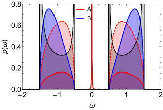
Figure 2: Bulk (black) and surface (red and blue) DOS for the isolated dimers chain. The solid lines correspond to the topological phase ($t_{1}/t_{2}=0.5$) and the dashed lines to the trivial one ($t_{1}/t_{2}=2$); for the B site the S-DOS overlap, as the only difference between the trivial and the topological is in the zero energy mode at A. The bulk DOS shows the gap between the conduction and valence band, as well as the Van Hove singularities expected from the flat dispersion at the top/bottom of the bands.

As expected for $t_{1}/t_{2}<1$, the S-DOS at site $A$ shows a zero-energy mode due to the topological nature of the system and the open boundary conditions. This effect is well known and was first predicted in polyacetylene chainsSSH-1979 , where the phonon field exhibits a degenerate ground state (two dimerization states) with solitonic excitations, and the coupling of the electrons to the solitons induces pairs of domain walls with localized electronic modes. In our model, the domain walls are created by a change in the hopping parameter, which is equivalent to a spatial modulation of the mass of the fermionic field. The topological properties of this system in equilibrium have been widely discussed in the literatureHatsugai , and its non-equilibrium counterpart is well understood for the case of an isolated chainAlviDimers ; Delplace-QuantumWalk . In equilibrium and for nearest neighbors hopping the two different topological phases can be characterized by a winding number $\nu_{1}=\left\{0,1\right\}$ depending on the ratio $t_{1}/t_{2}$. When $\nu_{1}=1$ the system is said to be topological and displays localized edge modes as the one seen in Fig.2. Out of equilibrium the classification is more complicated, and the appearance of two unequivalent gaps in the Floquet quasi-energy spectrum leads to a topological index $\mathbb{Z}\times\mathbb{Z}$Chiral-QWalks ; Delplace-QuantumWalk . In this work we will not calculate the topological invariants, but rather we will focus on their experimental signatures in the DOS, and on the differences in the transport properties between the topological and the non-topological phases.

We now discuss the effect of hybridization with the metallic contact for the case of nearest neighbors hopping $\lambda_{j;i,\sigma}=\lambda\delta_{i,j}\delta_{\sigma,A}$ (we choose this specific form for all calculations, but the generalization to a larger number of neighbors is straightforward). Intuitively, one would guess that if we start with our system in the topological phase ($t_{1}/t_{2}<1$), as the isolated edge state directly couples to the contact, it would be the one mostly affected. This is precisely what happens, especially for $\lambda\ll t_{3}$, where we find that the main effect in the S-DOS is the widening of the zero energy mode, although it remains well defined up to $\lambda\sim 0.1t_{3}$ (see Fig.3). Larger values of $\lambda$ smear out the zero energy mode until $\lambda\sim t_{3}$, where it merges with the continuum and any signature of the zero energy mode disappears. More counter-intuitive is the fact that the opposite process can also happen, where the A atom of the trivial phase hybridizes with the contact and B becomes the effective last site of the chain. This is equivalent to changing the dimerization ground state, and transforms the system into its topological phase, with the appearance of a zero energy mode at site B.

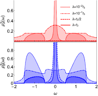
Figure 3: S-DOS at the A(B) site for $t_{1}/t_{2}=0.5\left(2\right)$ (up/down, respectively) and different values of $\lambda$. The initially topological phase becomes trivial when the A atom hybridizes with the contact. In opposition, for the trivial phase a zero energy mode emerges as $\lambda$ increases; this is because the hybridization exchanges the dimerized phase ($t_{1}\leftrightarrow t_{2}$).

Now that we have characterized our system properties in equilibrium we discuss the effect of the AC field. The reason why we do not initially consider the temporal gauge in Eq.1 is based on the absence of translational symmetry for a semi-infinite chain, however, the transformation to the interaction picture will still help us to encode the effect of the AC field in the hopping, and simplify the calculations. The transformation leads to the following time dependent Hamiltonian:

$$\tilde{H}\left(t\right) = \tilde{H}_{D}\left(t\right)+H_{C}+\tilde{H}_{T}\left(t\right)$$ (7)

$$\tilde{H}_{D}\left(t\right) = -\sum_{i,j,\alpha,\beta}\tilde{t}_{i,j}^{\alpha,\beta}\left(t\right)d_{i,\alpha}^{\dagger}d_{j,\beta}$$ (8)

$$\tilde{H}_{T}\left(t\right) = \sum_{j,i,\sigma}\left[\tilde{\lambda}_{j;i,\sigma}^{\ast}\left(t\right)c_{j}^{\dagger}d_{i,\sigma}+\tilde{\lambda}_{j;i,\sigma}\left(t\right)d_{i,\sigma}^{\dagger}c_{j}\right]$$ (9)

where the time dependent terms are $\tilde{t}_{i,j}^{\alpha,\beta}\left(t\right)=t_{i,j}^{\alpha,\beta}e^{iq\left(x_{i,\alpha}-x_{j,\beta}\right)\int V_{0}\left(t\right)dt}$ and $\tilde{\lambda}_{j;i,\sigma}\left(t\right)=\lambda_{j;i,\sigma}e^{iqx_{i,\sigma}\int V_{0}\left(t\right)dt}$. In the presence of a time dependent field, the Green’s functions now depend on $t$ and $t^{\prime}$ independently (do not confuse the time coordinate with the hopping parameters $t_{1,2,3}$); however the time periodicity of the Hamiltonain ensures that $\hat{G}\left(t+T,t^{\prime}+T\right)=\hat{G}\left(t,t^{\prime}\right)$. This symmetry can be used in our advantage if we consider Wigner coordinates $t_{+}=\left(t+t^{\prime}\right)/2$ and $t_{-}=t-t^{\prime}$, which imply that $\hat{G}\left(t_{-},t_{+}+T\right)=\hat{G}\left(t_{-},t_{+}\right)$. We define the Floquet-Green’s function asAoki2014-DMFT :

$$\hat{G}_{mn}\left(\omega\right)\equiv\frac{1}{T}\int_{0}^{T}dt_{+}e^{i\left(m-n\right)\Omega t_{+}}\hat{G}\left(\omega+\frac{m+n}{2}\Omega,t_{+}\right)$$ (10)

with $\hat{G}\left(\omega,t_{+}\right)=\int_{-\infty}^{\infty}e^{i\omega t_{-}}\hat{G}\left(t_{+},t_{-}\right)dt_{-}$. The advantage of this representation is two fold: it separates long time and short time dynamics, which allows for a simple physical interpretation, and transforms time convolutions into matrix products. Then one has the following simple form for the Dyson’s equation:

$$\hat{G}_{mn}\left(\omega\right)=\hat{g}_{mn}\left(\omega\right)+\sum_{m^{\prime}n^{\prime}}\hat{g}_{mm^{\prime}}\left(\omega\right)\hat{\Sigma}_{m^{\prime}n^{\prime}}\left(\omega\right)\hat{G}_{n^{\prime}n}\left(\omega\right)$$ (11)

which highly simplifies the calculations of the time dependent surface Green’s functions. We now study the effect of the AC field on both, the bulk and the surface Floquet-Green’s functions of the dimers chain. For the explicit calculations we fix $V_{0}\left(t\right)=V_{0}\cos\left(\Omega t\right)$, although the formalism allows for more general AC fields. The calculation of the bulk Green’s functions is done using the equation of motion technique (details in the Appendix), while for the case of the surface Green’s functions we consider Eq.11 to find the unperturbed surface Green’s function of the dimers chain, and then we add the effect of the metallic contact via the self-energy. For the bulk Green’s function $G_{k}^{\alpha,\beta}\left(t,t^{\prime}\right)=-i\theta\left(t-t^{\prime}\right)\langle\left\{d_{k,\alpha}\left(t\right),d_{k,\beta}^{\dagger}\left(t^{\prime}\right)\right\}\rangle$, where $k$ is a good quantum number due to the periodic boundary condition, we find the next hierarchy of equations in Wigner coordinates (remember that $\alpha,\beta=\pm$ refers to the sublattice degree of freedom):

$$\left(n\frac{\Omega}{2}+\omega\right)G_{k;n}^{\alpha,\beta}\left(\omega\right)=\delta_{n,0}\delta_{\alpha,\beta}-t_{1}G_{k;n}^{-\alpha,\beta}\left(\omega\right)\\ -t_{2}\sum_{l}\mathcal{J}_{\alpha l}\left(\xi\right)e^{i\alpha k}G_{k;n+l}^{-\alpha,\beta}\left(\omega+l\frac{\Omega}{2}\right)$$ (12)

where $\mathcal{J}_{n}\left(\xi\right)$ is the $n$-th Bessel function of the first kind and $\xi=qV_{0}/\Omega$. Note that the terms with $l\neq 0$ correspond to photon assisted tunneling, and lead to the appearance of side-bands. Importantly, the coupling to different side-bands rapidly decreases if $\Omega$ is the dominant energy scale, as contributions to the DOS from processes absorbing/emitting a photon with $n\Omega$ energy are proportional to $\mathcal{J}_{n}^{2}\left(\xi\right)/\Omega^{2}$. In this work we focus on high/intermediate frequency regimes $\Omega\apprge t_{1,2}$, as this configuration shows interesting propertiesAlviDimers ; however our calculation includes arbitrary photon transitions until we find numerical convergence, and can be used to study lower frequency regimes. If to lowest approximation, we neglect transitions to different side-bands, we find the usual result, viz. a renormalization of the hopping $t_{2}$ by $\mathcal{J}_{0}\left(\xi\right)$. This means that the DOS gets squeezed as the field amplitude increases, and for a zero of the Bessel function, the system displays flat bands. When we include higher order photon processes the renormalization is accompanied by the appearance of side-bands at multiples $\omega=n\Omega$, which can be observed in the time averaged DOS (Fig.4 shows the appearance of the first side-bands around $\omega=\pm 2.5$), and create extra transport channels which result in the Floquet sum rule for the conductivityFloquetSumRule .

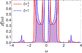
Figure 4: Bulk time averaged DOS for different values of the AC field amplitude $\xi$. The AC induces side-bands at $\omega=n\Omega$ and the field amplitude $\xi$ controls their width. Note that as we increase $\xi$, the gap size decreases, and for $t_{2}\mathcal{J}_{0}\left(\xi\right)=t_{1}$ we obtain the DOS of a linear chain. An increase of $\xi$ increases the spectral weight of the other side-bands. We have chosen $\Omega=4$ and $t_{1}=0.5$, in units of $t_{2}$.

We now discuss the surface Green’s functions in the presence of driving. As we previously discussed, they are calculated using Eq.11 and the Floquet form of the time-dependent self energy $\Sigma\left(t,t^{\prime}\right)$, which couples the $B$ site of an isolated dimer to the $A$ atom of the semi-infinite chain. Then, one can include the effect of the metallic contact by direct matrix inversion of the corresponding Dyson’s equation. In Fig.5 we show the presence of a zero-energy mode when $t_{1}/t_{2}\mathcal{J}_{0}\left(\xi\right)<1$, meaning that the coupling to the AC field does not destroy the initial topological phase due to the interaction between side-bands. Furthermore, we also find “zero-energy modes” at multiples of $\omega=n\Omega$, not only for the $A$ site, but for the $B$ site as well (only at $n\neq 0$, see Fig.5). This feature indicates that the edge states and topological phases of non-equilibrium systems are, in general, different to those in undriven systemsChiral-QWalks ; Benito2014 ; Delplace-QuantumWalk . The fact that the zero-energy modes at the $B$ site do not appear in the $n=0$ side-band indicates that they occur dynamically, and therefore possess an intrinsic time dependence. However, the oscillations between the $A$ and $B$ site of the last dimer still correspond to a localized zero-energy mode in the last dimer of the chain. The occupation of both sub-lattices in the presence of driving can be understood in terms of the extra symmetries present in periodically driven systemsChiral-QWalks . Importantly in our calculation, the domain walls are infinitely far and there is no hybridization between them; the effect corresponds to a purely dynamical one that persists in the thermodynamic limit.

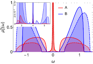
Figure 5: Time averaged S-DOS for the AC driven dimers chain and field strength $\xi=\left\{0.5,1\right\}$(dashed and solid, respectively). Note that the driving induces side-bands centered at frequency multiples $\omega=n\Omega$ which display localized modes as well (inset), but in contrast with the undriven case, the $B$ site also has a finite spectral weight. For this plot we have chosen $t_{1}=0.5$, $\lambda=0.01$ and $\Omega=4$ (in units of $t_{2}$).

The previous results show that the AC field produces several effects: 1) the bandwidth is renormalized by the field intensity, and this can produce metal-insulator transitions due to the appearance/disappearance of gaps; 2) the side-band structure implies the appearance of new transport channels; and 3) it can drive topological phase transitions with properties different to those of systems in thermal equilibrium. For the characterization of these changes, we calculate the current when the system is coupled to a metallic contact. We also describe how hybridization between the two systems $\lambda$ influences the current, and how the presence of zero-energy modes is captured in the current profile. For this, we calculate the current operatorJauho1993 :

$$J\left(t\right)=2q\sum_{i,j,\sigma}\Re\left\{\lambda_{j;\sigma,i}\left(t\right)G_{j;i,\sigma}^{<}\left(t,t\right)\right\}$$ (13)

being $G_{j;i,\sigma}^{<}\left(t,t^{\prime}\right)=i\langle d_{i,\sigma}^{\dagger}\left(t^{\prime}\right)c_{j}\left(t\right)\rangle$ the mixed lesser Green’s function, and $\lambda_{j;\sigma,i}\left(t\right)$ the tunneling between the contact and the dimers chain. We can separate the mixed Green’s function using the Langreth rules:

$$J\left(t\right) = 2q\int_{-\infty}^{\infty}\Re\left\{G_{0,A}^{r}\left(t,t_{1}\right)\Sigma_{0,A}^{<}\left(t_{1},t\right)\right.$$ (14)

$$\left.+G_{0,A}^{<}\left(t,t_{1}\right)\Sigma_{0,A}^{a}\left(t_{1},t\right)\right\}dt_{1}$$

where we have fixed $\lambda_{j;i,\sigma}=\lambda\delta_{i,j}\delta_{\sigma,A}$, $\Sigma_{0,A}^{a}\left(t_{1},t\right)=\left|\lambda\right|^{2}\mathfrak{g}_{0}^{a}\left(t_{1},t\right)$, $\Sigma_{0,A}^{<}\left(t_{1},t\right)=\left|\lambda\right|^{2}\mathfrak{g}_{0}^{<}\left(t_{1},t\right)$, $\mathfrak{g}_{0}\left(t_{1},t\right)$ is the unperturbed surface Green’s function of the linear chain, and $G_{0,A}\left(t,t_{1}\right)$ is the full surface Green’s function of the dimers chain. Due to the time periodicity, the expression for the current can be reduced to matrix products in Floquet representation:

$$J_{mn} = 2q\int_{-\infty}^{\infty}\sum_{k}\Re\left\{G_{mk}^{r}\left(\omega\right)\Sigma_{kn}^{<}\left(\omega\right)\right.$$ (15)

$$+\left.G_{mk}^{<}\left(\omega\right)\Sigma_{kn}^{a}\left(\omega\right)\right\}d\omega$$

where for simplicity we have included just the Floquet indices. In this work we assume that the dimers chain is driven out of equilibrium by the AC field, while the contact is in equilibrium at some chemical potential $\mu_{L}$. In this case, all time independent terms become diagonal in Floquet indices.

We first describe the I-V curves in the static case and the influence of hybridization with the metallic contact. In Fig.6 we plot the large bias current as a function of $\lambda$, for the topological and the trivial phase. It shows that the presence of the edge state lowers the average current, but it is still finite due to a finite DOS at finite energy. We observe that the difference between the two is especially large near the weak coupling limit $\lambda\ll t_{1},t_{2}$, as they scale very differently around $\lambda=0$Benito-AC-Dimers . The main reason for this decrease is the strong localization of the edge state, and the fact that it is the one that directly couples the dimers chain to the metallic contact. The inset shows the I-V curves for different values of $\lambda$, which show that all curves collapse to a single one in the strong coupling limit. It is also important that the contribution of the edge state to the current is infinitesimally small, as the domain wall provides just one electron to the current. Therefore, its presence contributes with an infinitesimal change in the current at $\mu_{L}=0$. Furthermore, the broadening of the mode due to hybridization does not seem to be captured in the I-V plot, which makes its detection more difficult. Finally, we have previously seen that the topological phase could be driven from the trivial one by hybridization with the contact. Unfortunately, this process is accompanied by a decrease in the S-DOS at the A site (now highly hybridized with the contact), decreasing the current and making more difficult the detection of the transition. Nevertheless we will show below that the dependence of the current on the field amplitude $\xi$, can help us to discriminate between the different phases.

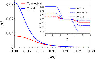
Figure 6: Average current vs coupling strength to the contact, for the topological($t_{1}=0.5t_{2}$) and trivial($t_{1}=2t_{2}$) phase (red and blue, respectively). For weak coupling we find a strong suppression of the current in the topological phase, related with the presence of a localized mode and a small S-DOS at site A (see Fig.2). Increasing $\lambda$ supresses the current in both cases, consequence of a decrease in the total S-DOS. We have chosen $t_{3}=100$ in units of $t_{2}$. The inset shows the I-V curve for different $\lambda$.

We now focus on the non-equilibrium case and discuss the average current and the I-V curve, as a function of the AC field parameters and for different coupling strengths to the metallic contact. In Fig.7 we plot the time average current as a function of the field amplitude $\xi$ for large bias and large $\Omega$. The top figure corresponds to the weak coupling limit ($\lambda=10^{-3}t_{3}$), where the dimers chain is slightly hybridized with the contact. It can be seen that, in the trivial phase, increasing the field amplitude does not affect the average current(blue solid line, for $t_{1}/t_{2}=2$), and it remains constant until the first zero of $\mathcal{J}_{0}\left(\xi\right)$, where the current suddenly drops to zero. This is equivalent to the well known coherent destruction of tunneling mechanismCDT1 ; CDT4 ; CDT5 ; CDT2 ; CDT3 , where the dimers decouple. On the other hand, the topological phase (red dashed line, for $t_{1}/t_{2}=0.5$) shows a continuous variation of the current as a function of $\xi$ due to the presence of the edge state. In this case, an increase of $\xi$ continuously reduces the gap between the conduction and the valence band, and it is easier for an electron localized in the edge state to jump to one of the bulk bands, increasing the current. At $\xi\simeq 1.5$ the two bands close the gap, the phase becomes trivial, and then insensitive to changes of $\xi$. The bottom figure plots the case of large hybridization with the contact ($\lambda=t_{3}$), where as we previously discussed, the role of the topological and trivial phase has been inverted, but the current in the absence of the AC field could not distinguish between the two of them. It turns out that as the AC field amplitude increases, both cases show the same behavior as in the weak coupling case, ie. the current in the presence of a localized state continuously changes with $\xi$, while the current for the phase without an edge state is locked until the bands close the gap again. This shows that the $\xi$ dependence of the time averaged current can be used as a tool to detect the presence of localized modes in the chain.

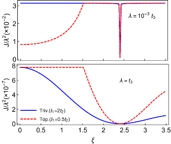
Figure 7: Large bias current vs $\xi$, for weak and strong (top and bottom, respectively) coupling to the metallic contact. The current responds continuously to variations of the field amplitude if the dimers chain has a localized energy mode, while the trivial phase is insensitive. We have chosen $\Omega$ twice as large as the undriven bandwidth and $t_{3}=100$, in units of $t_{2}$.

Finally, we analyze the I-V curves for different parameters of the AC field; they are shown in Fig.8. The comparison between the equilibrium and out-of-equilibrium case (solid and dashed, respectively) shows how the large bias current is unaffected within the trivial phase (blue), while for the topological phase increases to almost twice its original value; also, the renormalization of the bands can be observed as an increase in the slope of the curves. The inset shows that the current can capture the side-band structure previously discussed, as the AC field induces new transport channels at multiples of the driving frequency. In the high frequency regime, which is discussed in this work, their contribution to the current is small; however, their presence will increase as the system approaches resonance. It is also important to notice that, as for the undriven case, the edge states at $\omega=n\Omega$ are absent from the I-V curves due to their small spectral weight.

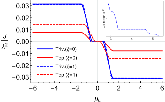
Figure 8: Time average current as a function of the chemical potential $\mu_{L}$. The solid lines correspond to the current in absence of driving, and the dashed lines correspond to the average current for $\xi=1$ and $\Omega=4$. The inset shows a zoom of the current when $\mu_{L}$ is measuring the contribution from the photo-induced side-bands. We have chosen $\lambda=10^{-2}$ and $t_{3}=100$, in units of $t_{2}$.

Conclusions:

We have studied the non-equilibrium properties of a semi-infinite dimers chain coupled to both, an AC electric field and to a metallic contact at a different chemical potential. Combining Keldysh formalism with the surface Green’s functions method for semi-infinite systems we have studied the thermodynamic limit, where finite size effects do not affect the edge states or transport properties. Furthermore, the formalism allows us to obtain results in the case of large hybridization between the dimers chain and the metallic contact (strong coupling limit). We find that with this method we can calculate to arbitrary accuracy the surface Green’s functions of the system, and therefore analyze the fate of the edge states in a non-equilibrium topological phase, and their contribution to the current. For the equilibrium case we find that the strong coupling limit can alter the topological properties of the dimers chain, as the hybridization with the metallic contact can change the dimerization ground state of the system. We find the characteristic current suppression and edge-state blockade of a system with edge states for the case of small hybridization with the contactBenito-AC-Dimers ; however, we have shown that as the hybridization increases, this effect gets reduced, making more difficult the distinction between the trivial and the topological phase. In the presence of the high frequency AC field we have found that the equilibrium edge states, which are initially localized in one sub-lattice, gain spectral weight in the opposite one, and show the appearance of side-bands, which contribute as extra transport channels. Importantly, we have found that the average current shows a different behavior, as a function of the AC field amplitude, when the dimers chain has an edge state; in the trivial phase the current is slightly affected by a change in the field amplitude, while the topological phase shows a continuous variation of the average current due to the hybridization between the edge state and the bulk bands. Furthermore, this property seems to hold for large hybridization with the metallic contact, which could be very helpful in a realistic situation.

The study of intermediate frequencies would be interesting for future works, as the topological properties change once different side-bands cross. The adiabatic regime is also of interest, with the inclusion of multi-frequency fields to simulate higher dimensional propertiesMultiFreq . Extensions of this work including domain wall dynamics would also be interesting for applications in molecular electronics, where the dynamics of solitons has been proposed to build molecular switches, transistors and memoriesSolitonSwitch . In this case, one could take advantage of the external control provided by the AC field, and combine the soliton dynamics with the external control of the coupling to the electrons. Finally, although we have not discussed the effect of dissipation and heating in the system, it can be important in periodically driven systems and would require an analysis including a dissipative bosonic and fermionic bath; however, this discussion is out of the scope of the present manuscript and would require a more detailed description of a concrete setup in order to include all the relevant decoherence mechanismsMitra1 ; PhysRevX.5.041050 ; Chamon1 ; Dissipation1 .

We would like to acknowledge P.C.E. Stamp, G. Platero, and M. Benito for the critical reading of the manuscript. This work was supported by NSER of Canada and MAT2014.

Appendix A Surface Green’s functions for semi-infinite chains

In this section we calculate the surface Green’s functions for the linear and the dimers chain. We mention that the surface Green’s functions are interesting because they can be calculated exactly, and they provide information about boundary states in systems with hardwall conditions. For the calculation of the surface Green’s functions we just need to consider Dyson’s equation and the recurrence relation obtained in a semi-infinite system. Let us begin with the metallic contact, modeled by a tight binding Hamiltonian:

$$H_{C}=\mu_{L}\sum_{i=0}^{\infty}n_{i}-t_{3}\sum_{\langle i,j\rangle}c_{i}^{\dagger}c_{j}+h.c.$$ (16)

If we consider the case of the $x_{0}$ site initially decoupled from the chain (i.e., $c_{0}^{\dagger}c_{1}$ and $c_{1}^{\dagger}c_{0}$ are removed from the Hamiltonian), and we re-attach it, the process can be described with the Dyson’s equation $\hat{\mathfrak{g}}=\hat{\mathfrak{g}}^{\left(0\right)}+\hat{\mathfrak{g}}^{\left(0\right)}\cdot\hat{V}\cdot\hat{\mathfrak{g}}$, where $\hat{\mathfrak{g}}^{\left(0\right)}$ is the Green’s function for the two systems initially decoupled, $\hat{\mathfrak{g}}$ is the Green’s function for the system when they are coupled, and $\hat{V}$ is the hopping between the sites $0$ and $1$. In matrix form, the Dyson’s equation reads:

$$\left(\begin{array}[]{cc}\mathfrak{g}_{0}&\mathfrak{g}_{01}\\ \mathfrak{g}_{10}&\mathfrak{g}_{1}\end{array}\right)=\left(\begin{array}[]{cc}\mathfrak{g}_{0}^{\left(0\right)}&0\\ 0&\mathfrak{g}_{1}^{\left(0\right)}\end{array}\right)+\left(\begin{array}[]{cc}\mathfrak{g}_{0}^{\left(0\right)}&0\\ 0&\mathfrak{g}_{1}^{\left(0\right)}\end{array}\right)\left(\begin{array}[]{cc}0&-t_{3}\\ -t_{3}&0\end{array}\right)\left(\begin{array}[]{cc}\mathfrak{g}_{0}&\mathfrak{g}_{01}\\ \mathfrak{g}_{10}&\mathfrak{g}_{1}\end{array}\right)$$ (17)

where $\mathfrak{g}_{1}^{\left(0\right)}$ corresponds to the unperturbed surface Green’s function at site $1$ of the semi-infinite chain. The equation for $\mathfrak{g}_{0}$ results in:

$$\mathfrak{g}_{0}= \mathfrak{g}_{0}^{\left(0\right)}-\mathfrak{g}_{1}^{\left(0\right)}t_{3}\mathfrak{g}_{10}=\mathfrak{g}_{0}^{\left(0\right)}+t_{3}^{2}\mathfrak{g}_{0}^{\left(0\right)}\mathfrak{g}_{1}^{\left(0\right)}\mathfrak{g}_{0}$$ (18)

where we have used $\mathfrak{g}_{10}=-t_{3}\mathfrak{g}_{1}^{\left(0\right)}\mathfrak{g}_{0}$. Finally, noticing that after attaching the site $0$ to the semi-infinite chain, $\mathfrak{g}_{1}^{\left(0\right)}=\mathfrak{g}_{0}$ we obtain a second order equation with solution:

$$\mathfrak{g}_{0}\left(\omega\right)=\frac{1\pm\sqrt{1-4t_{3}^{2}\left[\mathfrak{g}_{0}^{\left(0\right)}\left(\omega\right)\right]^{2}}}{2t_{3}^{2}\mathfrak{g}_{0}^{\left(0\right)}\left(\omega\right)}$$ (19)

Finally, we use the single site Green’s function $\mathfrak{g}_{0}^{\left(0\right)}=\left(\omega-\mu_{L}\right)^{-1}$ and find:

$$\mathfrak{g}_{0}\left(\omega\right)=\frac{\omega-\mu_{L}}{2t_{3}^{2}}\left[1\pm\sqrt{1-\left(\frac{2t_{3}}{\omega-\mu_{L}}\right)^{2}}\right]$$ (20)

where we can fix the minus sign in order to obtain the right density of states:

$$\rho\left(\omega\right)=-\frac{1}{\pi}\lim_{\epsilon\rightarrow 0^{+}}\Im\left\{\mathfrak{g}_{0}\left(\omega+i\epsilon\right)\right\}$$ (21)

which is non-vanishing when $\left|\omega-\mu_{L}\right|<2t_{3}$. For the case of a dimers chain one can proceed in a similar way, this time including a sub-lattice degree of freedom.

Appendix B Floquet Green’s functions

Here we calculate the Floquet-Green’s function for the dimers chain coupled to an AC field. We define the dimers chain Green’s function and its Wigner form as ($t_{+}=\left(t+t^{\prime}\right)/2$ and $t_{-}=t-t^{\prime}$):

$$G_{k}^{\mu,\nu}\left(t,t^{\prime}\right) =-i\theta\left(t-t^{\prime}\right)\langle\left\{d_{k,\mu}\left(t\right),d_{k,\nu}^{\dagger}\left(t^{\prime}\right)\right\}\rangle$$ (22)

$$G\left(t_{+},t_{-}\right) =\frac{1}{2\pi}\int d\omega e^{-i\omega t_{-}}\sum_{n}e^{-in\Omega t_{+}}G_{n}\left(\omega\right)$$ (23)

$$G_{n}\left(\omega\right) =\int e^{i\omega t_{-}}dt_{-}\frac{1}{T}\int_{0}^{T}e^{in\Omega t_{+}}G\left(t_{+},t_{-}\right)dt_{+}$$ (24)

which corresponds to the propagation of a fermion with momentum $k$ under the Hamiltonian:

$$\tilde{H}_{D}\left(t\right) = \mu_{D}\sum_{\alpha,i}d_{i,\alpha}^{\dagger}d_{i,\alpha}-\sum_{i,j,\alpha,\beta}\tilde{t}_{i,j}^{\alpha,\beta}\left(t\right)d_{i,\alpha}^{\dagger}d_{j,\beta}=\mu_{D}\sum_{\alpha,\mathbf{k}}n_{\mathbf{k},\alpha}-\sum_{k,\alpha,\beta}\hat{t}_{k}^{\alpha,\beta}\left(t\right)d_{k,\alpha}^{\dagger}d_{k,\beta}$$ (25)

where the time dependent hoppings are $\tilde{t}_{i,j}^{\alpha,\beta}\left(t\right)=t_{i,j}^{\alpha,\beta}e^{i\xi\left(x_{i,\alpha}-x_{j,\beta}\right)\sin\left(\Omega t\right)}$ and $\xi=\frac{qV_{0}}{\Omega}$, and concretely in our case:

$$\hat{t}_{k}^{\alpha,\beta}\left(t\right)=\left(\begin{array}[]{cc}0&t_{1}+t_{2}e^{i\left(k+\xi\sin\left(\Omega t\right)\right)}\\ t_{1}+t_{2}e^{-i\left(k+\xi\sin\left(\Omega t\right)\right)}&0\end{array}\right)=\left(\begin{array}[]{cc}0&t_{1}+t_{2}e^{ik}\sum_{l}J_{l}\left(\xi\right)e^{il\Omega t}\\ t_{1}+t_{2}e^{-ik}\sum_{l}J_{-l}\left(\xi\right)e^{il\Omega t}&0\end{array}\right)$$ (26)

The equation of motion for the Green’s function is given by:

$$\left(\frac{i}{2}\partial_{t_{+}}+i\partial_{t_{-}}-\mu_{D}\right)G_{k}^{\mu,\nu}\left(t_{+},t_{-}\right) = \delta_{\mu,\nu}\delta\left(t_{-}\right)-\hat{t}_{k}^{\mu,-\mu}\left(t\right)G_{k}^{-\mu,\nu}\left(t_{+},t_{-}\right)$$ (27)

and Fourier transforming to frequency space we finally get ($\mu,\nu=A,B$):

$$\left(n\frac{\Omega}{2}+\omega-\mu_{D}\right)G_{k;n}^{\mu,\nu}\left(\omega\right) = \delta_{n,0}\delta_{\mu,\nu}-t_{1}G_{k;n}^{-\mu,\nu}\left(\omega\right)-t_{2}\sum_{l}\mathcal{J}_{\mu l}\left(\xi\right)e^{i\mu k}G_{k;n+l}^{-\mu,\nu}\left(\omega+l\frac{\Omega}{2}\right)$$ (28)

Therefore, the equation for the $n=0$ Green’s function is:

$$\left(\omega-\mu_{D}\right)G_{k;0}^{\mu,\nu}\left(\omega\right) = \delta_{\mu,\nu}-t_{1}G_{k;0}^{-\mu,\nu}\left(\omega\right)-t_{2}\sum_{l}\mathcal{J}_{\mu l}\left(\xi\right)e^{i\mu k}G_{k;l}^{-\mu,\nu}\left(\omega+l\frac{\Omega}{2}\right)$$ (29)

and the general equation of motion, for all the Green’s functions included in the calculation, is:

$$\left(\omega+l\Omega-\mu_{D}\right)G_{k;l}^{\mu,\nu}\left(\omega+l\frac{\Omega}{2}\right) = \delta_{l,0}\delta_{\mu,\nu}-t_{1}G_{k;l}^{-\mu,\nu}\left(\omega+l\frac{\Omega}{2}\right)-t_{2}\sum_{r}\mathcal{J}_{\mu r}\left(\xi\right)e^{i\mu k}G_{k;l+r}^{-\mu,\nu}\left(\omega+\left(l+r\right)\frac{\Omega}{2}\right)$$ (30)

This system of equations can be solved to arbitrary accuracy and mapped into the Floquet representation. The calculation of the AC driven surface Green’s functions is similar, but we need to consider the Dyson’s equation to represent the process of coupling the single site to the semi-infinite chain, and this time, a self-energy which is time dependent. The Dyson’s equation is given by:

$$\hat{G}\left(t,t^{\prime}\right)=\hat{g}\left(t,t^{\prime}\right)+\int dt_{1}\int dt_{2}\hat{g}\left(t,t_{1}\right)\hat{\Sigma}\left(t_{1},t_{2}\right)\hat{G}\left(t_{2},t^{\prime}\right)$$ (31)

where:

$$\hat{G}\left(t,t^{\prime}\right) = \left(\begin{array}[]{cc}\hat{G}_{0}\left(t,t^{\prime}\right)&\hat{G}_{0C}\left(t,t^{\prime}\right)\\ \hat{G}_{C0}\left(t,t^{\prime}\right)&\hat{G}_{C}\left(t,t^{\prime}\right)\end{array}\right)$$ (34)

$$\hat{g}\left(t,t^{\prime}\right) = \left(\begin{array}[]{cc}\hat{g}_{0}\left(t,t^{\prime}\right)&0\\ 0&\hat{G}_{0}\left(t,t^{\prime}\right)\end{array}\right)$$ (37)

$$\hat{\Sigma}\left(t,t^{\prime}\right) = \left(\begin{array}[]{cc}0&\tilde{t}\left(t\right)\\ \tilde{t}\left(t\right)^{\ast}&0\end{array}\right)\delta\left(t-t^{\prime}\right)$$ (40)

and we have defined $\tilde{t}\left(t\right)=\tilde{t}e^{i\xi\sin\left(\Omega t\right)}$ and $\tilde{t}$ is a matrix in the sub-lattice indices for the case of a dimers chain. In order to deal with this integral equation it is useful to go to the Floquet representation:

$$\hat{G}_{mn}\left(\omega\right) \equiv\hat{G}_{m-n}\left(\omega+\frac{m+n}{2}\Omega\right)$$ (41)

$$\hat{g}_{mn}\left(\omega\right) \equiv\hat{g}_{m-n}\left(\omega+\frac{m+n}{2}\Omega\right)$$ (42)

$$\hat{\Sigma}_{mn}\left(\omega\right) \equiv\hat{\Sigma}_{m-n}\left(\omega+\frac{m+n}{2}\Omega\right)$$ (43)

where the Dyson’s equation transforms into a matrix multiplication:

$$\hat{G}_{mn}\left(\omega\right)=\hat{g}_{mn}\left(\omega\right)+\sum_{m^{\prime}n^{\prime}}\hat{g}_{mm^{\prime}}\left(\omega\right)\hat{\Sigma}_{m^{\prime}n^{\prime}}\left(\omega\right)\hat{G}_{n^{\prime}n}\left(\omega\right)$$ (44)

For the explicit calculation of the dimers chain we need to calculate the Wigner transform of the self-energy, which leads to the next Floquet representation:

$$\hat{\Sigma}_{mn} =-t_{2}\left(\begin{array}[]{cccc}0&0&0&0\\ 0&0&\mathcal{J}_{n-m}\left(\xi\right)&0\\ 0&\mathcal{J}_{m-n}\left(\xi\right)&0&0\\ 0&0&0&0\end{array}\right)$$ (49)

With these expressions one can solve the Dyson’s equation for the surface Green’s function in presence of driving.

Appendix C Current calculation

In this Appendix we write the explicit expressions for the time dependent current through the hybrid system. For that we make use of the Keldysh formalism, which allows to treat the problem in a very simple and systematic way. We start by separating the total Hamiltonian into its central system, reservoir and tunneling parts:

$$H=H_{D}+H_{C}+H_{T}$$ (50)

For the current calculation we just need to focus in the tunneling Hamiltonian:

$$H_{T}=\sum_{i,j,\sigma}\left(\lambda_{j;\sigma,i}^{\ast}\left(t\right)c_{j}^{\dagger}d_{\sigma,i}+\lambda_{j;\sigma,i}\left(t\right)d_{\sigma,i}^{\dagger}c_{j}\right)$$ (51)

as the metallic contact and dimers chain Hamiltonians can be kept quite general for this discussion. To determine the current operator we begin by calculating the time variation of the number of particles in the reservoir $\hat{Q}=q\sum_{i}c_{i}^{\dagger}c_{i}$ ($\hbar=1$):

$$\hat{J}\left(t\right) =\partial_{t}\hat{Q}=iq\sum_{j\in R}\sum_{\sigma,i\in S}\left\{\lambda_{j;\sigma,i}\left(t\right)d_{i,\sigma}^{\dagger}c_{j}-\lambda_{j;\sigma,i}^{\ast}\left(t\right)c_{j}^{\dagger}d_{i,\sigma}\right\}$$ (52)

Therefore, the average current is related with the lesser Green’s functions:

$$G_{j,\alpha;l,\sigma}^{<}\left(t,t^{\prime}\right) =i\langle d_{l,\sigma}^{\dagger}\left(t^{\prime}\right)c_{j,\alpha}\left(t\right)\rangle$$ (53)

$$G_{l,\sigma;j,\alpha}^{<}\left(t,t^{\prime}\right) =i\langle c_{j,\alpha}^{\dagger}\left(t^{\prime}\right)d_{l,\sigma}^{\dagger}\left(t\right)\rangle$$ (54)

and can be rewritten as:

$$J\left(t\right)=2q\sum_{i,j,\sigma}\Re\left\{\lambda_{j;\sigma,i}\left(t\right)G_{j;i,\sigma}^{<}\left(t,t\right)\right\}$$ (55)

In conclusion, the time dependent current requires to calculate the equal time, lesser Green’s function $G_{j;i,\sigma}^{<}\left(t,t\right)$ only. Furthermore, as we will assume that the tunnel Hamiltonian connects the two sites at the end of each chain, the expression will only depend on the surface Green’s functions. Using the equation of motion technique and the Langreth rules for the contour ordered Green’s function, one can write the expression for the lesser Green’s function as:

$$G_{j;i,\sigma}^{<}\left(t,t\right)=\sum_{i^{\prime},\sigma^{\prime}}\int dt_{1}\lambda_{j;i^{\prime},\sigma^{\prime}}^{\ast}\left(t_{1}\right)\left[G_{i,\sigma;i^{\prime},\sigma^{\prime}}^{r}\left(t,t_{1}\right)\mathfrak{g}_{j}^{<}\left(t_{1},t\right)+G_{i,\sigma;i^{\prime},\sigma^{\prime}}^{<}\left(t,t_{1}\right)\mathfrak{g}_{j}^{a}\left(t_{1},t\right)\right]$$ (56)

were we have separated the mixed Green’s function into a product of surface Green’s functions, and $\mathfrak{g}$ corresponds to the unperturbed surface Green’s function of the metallic contact. The expression for the current becomes:

$$J\left(t\right)=2q\sum_{i,j,\sigma}\sum_{i^{\prime},\sigma^{\prime}}\int_{-\infty}^{\infty}dt_{1}\Re\left\{\lambda_{j;\sigma,i}\left(t\right)\lambda_{j;i^{\prime},\sigma^{\prime}}^{\ast}\left(t_{1}\right)\left[G_{i,\sigma;i^{\prime},\sigma^{\prime}}^{r}\left(t,t_{1}\right)\mathfrak{g}_{j}^{<}\left(t_{1},t\right)+G_{i,\sigma;i^{\prime},\sigma^{\prime}}^{<}\left(t,t_{1}\right)\mathfrak{g}_{j}^{a}\left(t_{1},t\right)\right]\right\}$$ (57)

and identifying the self-energies:

$$\Sigma_{i,\sigma;i^{\prime},\sigma^{\prime}}^{a}\left(t_{1},t\right) =\sum_{j}\lambda_{j;\sigma,i}\left(t\right)\lambda_{j;i^{\prime},\sigma^{\prime}}^{\ast}\left(t_{1}\right)\mathfrak{g}_{j}^{a}\left(t_{1},t\right)$$ (58)

$$\Sigma_{i,\sigma;i^{\prime},\sigma^{\prime}}^{<}\left(t_{1},t\right) =\sum_{j}\lambda_{j;\sigma,i}\left(t\right)\lambda_{j;i^{\prime},\sigma^{\prime}}^{\ast}\left(t_{1}\right)\mathfrak{g}_{j}^{<}\left(t_{1},t\right)$$ (59)

we obtain:

$$J\left(t\right)=2q\sum_{j,i,\sigma}\sum_{i^{\prime},\sigma^{\prime}}\int_{-\infty}^{\infty}\Re\left\{G_{i,\sigma;i^{\prime},\sigma^{\prime}}^{r}\left(t,t_{1}\right)\Sigma_{i,\sigma;i^{\prime},\sigma^{\prime}}^{<}\left(t_{1},t\right)+G_{i,\sigma;i^{\prime},\sigma^{\prime}}^{<}\left(t,t_{1}\right)\Sigma_{i,\sigma;i^{\prime},\sigma^{\prime}}^{a}\left(t_{1},t\right)\right\}dt_{1}$$ (60)

The problem of calculating the current for a time dependent system has been reduced to the calculation of the self-energies and Green’s functions for the dimers chain. The form of the previous expression allows for one further simplification when dealing with AC fields. We can consider the Floquet-Keldysh formalism and reduce the time integrals to matrix multiplications. For that purpose let us generalize the current operator to a two-2 time function:

$$J\left(t,t^{\prime}\right)=2q\sum_{i,j,\sigma}\sum_{i^{\prime},\sigma^{\prime}}\int_{-\infty}^{\infty}\Re\left\{G_{i,\sigma;i^{\prime},\sigma^{\prime}}^{r}\left(t,t_{1}\right)\Sigma_{i,\sigma;i^{\prime},\sigma^{\prime}}^{<}\left(t_{1},t^{\prime}\right)+G_{i,\sigma;i^{\prime},\sigma^{\prime}}^{<}\left(t,t_{1}\right)\Sigma_{i,\sigma;i^{\prime},\sigma^{\prime}}^{a}\left(t_{1},t^{\prime}\right)\right\}dt_{1}$$ (61)

which can be rewritten in Wigner coordinates as:

$$J\left(t_{+},t_{-}\right) = \sum_{l}\int_{-\infty}^{\infty}J_{l}\left(\omega\right)e^{-il\Omega t_{+}-i\omega t_{-}}\frac{d\omega}{2\pi}$$ (62)

$$J_{l}\left(\omega\right) = \frac{1}{T}\int_{0}^{T}dt_{+}\int_{-\infty}^{\infty}J\left(t_{+},t_{-}\right)e^{il\Omega t_{+}+i\omega t_{-}}dt_{-}$$ (63)

Therefore, the equal time current is given by:

$$J\left(t\right) = \sum_{l}e^{-il\Omega t}\int_{-\infty}^{\infty}J_{l}\left(\omega\right)\frac{d\omega}{2\pi}=\sum_{l}e^{-il\Omega t}J_{l}$$ (64)

obtained by the inverse Fourier transformed of $J_{l}\left(\omega\right)$ integrated over all frequencies $\omega$. Therefore, we just need to calculate the Floquet matrix (in the next expression we omit the site and sub-lattice indices for simplicity):

$$J_{mn}\left(\omega\right)=2q\sum_{k}\Re\left\{G_{mk}^{r}\left(\omega\right)\Sigma_{kn}^{<}\left(\omega\right)+G_{mk}^{<}\left(\omega\right)\Sigma_{kn}^{a}\left(\omega\right)\right\}$$ (65)

and integrate over all $\omega$ in order to obtain the different Fourier components of the current. Concretely for the constant contribution we just need to obtain the diagonal terms $m=n$.

As in our model we assume that the contact is in equilibrium, and that the tunneling $\lambda$ is time independent, the expressions for the self energies and the surface Green’s functions for the linear chain highly simplify:

$$\mathfrak{g}_{0}^{<}\left(\omega\right) = if\left(\omega\right)A_{0}\left(\omega\right)$$ (66)

$$\Sigma_{0,A}^{a}\left(\omega\right) = \left|\lambda\right|^{2}\mathfrak{g}_{0}^{a}\left(\omega\right)$$ (67)

$$\Sigma_{0,A}^{<}\left(\omega\right) = \left|\lambda\right|^{2}\mathfrak{g}_{0}^{<}\left(\omega\right)$$ (68)

where $f\left(\omega\right)=\left(e^{\beta\omega}+1\right)^{-1}$ is the Fermi function. Their representation in Floquet form is trivial, as it corresponds to a diagonal form. Therefore, for the calculation one just needs to include the full surface Green’s functions in Floquet form, obtained in the main text.

References

- (1) B. A. Bernevig, T. L. Hughes, and S. C. Zhang, Science (New York, N.Y.) 314, 1757 (2006).
- (2) X.-L. Qi and S.-C. Zhang, Phys. Today 63, 33 (2010).
- (3) M. Hasan and C. Kane, Reviews of Modern Physics 82, 3045 (2010).
- (4) A. Schnyder, S. Ryu, A. Furusaki, and A. Ludwig, Physical Review B 78, 195125 (2008).
- (5) L. Jiang et al., Phys. Rev. Lett. 106, 220402 (2011).
- (6) L. P. Rokhinson, X. Liu, and J. K. Furdyna, Nature Physics 8, 795 (2012).
- (7) S. Nadj-Perge, I. Drozdov, J. Li, and H. Chen, Science (New York, N.Y.) 10, 1 (2014).
- (8) J. Eisert, M. Friesdorf, and C. Gogolin, Nature Physics 11, 124 (2015).
- (9) P. Hauke et al., Phys. Rev. Lett. 109, 145301 (2012).
- (10) N. H. Lindner, G. Refael, and V. Galitski, Nature Physics 7, 490 (2011).
- (11) T. Kitagawa, T. Oka, A. Brataas, L. Fu, and E. Demler, Physical Review B 84, 235108 (2011).
- (12) Á. Gómez-León and G. Platero, Physical Review Letters 110, 200403 (2013).
- (13) Á. Gómez-León, P. Delplace, and G. Platero, Physical Review B 89, 205408 (2014).
- (14) M. Bello, C. E. Creffield, and G. Platero, Nature Publishing Group , 1 (2015).
- (15) Y. H. Wang, H. Steinberg, P. Jarillo-Herrero, and N. Gedik, Science 342, 453 (2013).
- (16) P. Delplace, Á. Gómez-León, and G. Platero, Phys. Rev. B 88, 245422 (2013).
- (17) A. G. Grushin, Á. Gómez-León, and T. Neupert, Physical Review Letters 112, 156801 (2014).
- (18) S. Ryu and Y. Hatsugai, Phys. Rev. Lett. 89, 077002 (2002).
- (19) P. Delplace, D. Ullmo, and G. Montambaux, Physical Review B 84, 195452 (2011).
- (20) W. P. Su, R. Schrieffer, and J. A. Heeger, Phys. Rev. Lett. 42, 1698 (1979).
- (21) W. P. Su, J. R. Schrieffer, and J. A. Heeger, Phys. Rev. B 22, 2099 (1980).
- (22) J. A. Heeger, S. Kivelson, J. R. Schrieffer, and W. P. Su, Reviews of Modern Physics 60, 781 (1988).
- (23) M. P. Groves, C. F. Carvalho, and R. H. Prager, Materials Science and Engineering: C 3, 181 (1995).
- (24) G. M. e Silva and P. H. Acioli, Synthetic Metals 87, 249 (1997).
- (25) T. Brandes, Physical Review B 56, 1213 (1997).
- (26) B. H. Wu and J. C. Cao, Journal of Physics: Condensed Matter 20, 085224 (2008).
- (27) H. Aoki et al., Reviews of Modern Physics 86 (2014).
- (28) M. Genske and A. Rosch, Phys. Rev. A 92, 062108 (2015).
- (29) F. Dolcini, Phys. Rev. B 85, 033306 (2012).
- (30) D. A. Ryndyk, R. Gutiérrez, B. Song, and G. Cuniberti, Green Function Techniques in the Treatment of Quantum Transport at the Molecular Scale, pages 213–335, Springer Berlin Heidelberg, Berlin, Heidelberg, 2009.
- (31) J. Velev and W. Butler, Journal of Physics: Condensed Matter 16, R637 (2004).
- (32) K. M. Seja, G. Kiršanskas, C. Timm, and A. Wacker, (2016).
- (33) S. Blanes, F. Casas, J. Oteo, and J. Ros, Physics Reports 470, 151 (2009).
- (34) A. Eckardt and E. Anisimovas, New Journal of Physics 17, 93039 (2015).
- (35) M. Bukov, L. D’Alessio, and A. Polkovnikov, Advances in Physics 64, 139 (2015).
- (36) M. Niklas, M. Benito, S. Kohler, and G. Platero, Nanotechnology 27, 454002 (2016).
- (37) M. Benito, M. Niklas, G. Platero, and S. Kohler, Phys. Rev. B 93, 115432 (2016).
- (38) Á. Gómez-León, Phys. Rev. B 94, 035144 (2016).
- (39) J. K. Asbóth, B. Tarasinski, and P. Delplace, Phys. Rev. B 90, 125143 (2014).
- (40) J. K. Asbóth and H. Obuse, Phys. Rev. B 88, 121406 (2013).
- (41) A. Kundu and B. Seradjeh, Phys. Rev. Lett. 111, 136402 (2013).
- (42) M. Benito, Á. Gómez-León, V. M. Bastidas, T. Brandes, and G. Platero, Physical Review B 90, 205127 (2014).
- (43) N. Wingreen, A. Jauho, and Y. Meir, Physical Review B 48, 8487 (1993).
- (44) F. Grossmann, T. Dittrich, P. Jung, and P. Hänggi, Phys. Rev. Lett. 67, 516 (1991).
- (45) M. Grifoni and P. Hanggi, Physics Reports 304, 229 (1998).
- (46) S. Kohler, J. Lehmann, and P. Hanggi, Physics Reports 406, 379 (2005).
- (47) A. Gómez-León and G. Platero, Phys. Rev. B 84, 121310 (2011).
- (48) A. Gómez-León and G. Platero, Phys. Rev. B 85, 245319 (2012).
- (49) J.-Y. Zou and B.-G. Liu, Arxiv Arxiv, 1611.01126 (2016).
- (50) H. Dehghani, T. Oka, and A. Mitra, Phys. Rev. B 90, 195429 (2014).
- (51) K. I. Seetharam, C.-E. Bardyn, N. H. Lindner, M. S. Rudner, and G. Refael, Phys. Rev. X 5, 041050 (2015).
- (52) T. Iadecola, T. Neupert, and C. Chamon, Phys. Rev. B 91, 235133 (2015).
- (53) D. E. Liu, A. Levchenko, and R. M. Lutchyn, Arxiv Arxiv, 1610.09105 (2016).