Optimal Dynamic Point Selection for Power Minimization in Multiuser Downlink CoMP

Abstract

This paper examines a CoMP system where multiple base-stations (BS) employ coordinated beamforming to serve multiple mobile-stations (MS). Under the dynamic point selection mode, each MS can be assigned to only one BS at any time. This work then presents a solution framework to optimize the BS associations and coordinated beamformers for all MSs. With target signal-to-interference-plus-noise ratios at the MSs, the design objective is to minimize either the weighted sum transmit power or the per-BS transmit power margin. Since the original optimization problems contain binary variables indicating the BS associations, finding their optimal solutions is a challenging task. To circumvent this difficulty, we first relax the original problems into new optimization problems by expanding their constraint sets. Based on the nonconvex quadratic constrained quadratic programming framework, we show that these relaxed problems can be solved optimally. Interestingly, with the first design objective, the obtained solution from the relaxed problem is also optimal to the original problem. With the second design objective, a suboptimal solution to the original problem is then proposed, based on the obtained solution from the relaxed problem. Simulation results show that the resulting jointly optimal BS association and beamforming design significantly outperforms fixed BS association schemes.

I Introduction

To improve the spectral efficiency, current designs of wireless networks adopt universal frequency reuse where all the cells can share the same radio spectrum resources. However, universal frequency reuse comes at the cost of severe intercell interference (ICI), especially at cell-edge mobile stations (MS). In the 3GPP LTE-Advanced standard, coordinated multi-point transmission/reception (CoMP) is considered as an enabling technique to actively deal with the ICI [2]. In CoMP, the coverage, throughput and efficiency of the multicell system can be significantly improved by fully coordinating and optimizing the concurrent transmissions from multiple base-stations (BS) to the MSs [2, 3]. Depending on the level of coordination among the coordinated cells, a CoMP system can operate under different modes, namely joint processing/joint transmission (JP/JT), dynamic point selection (DPS), and coordinated scheduling/coordinated beamforming (CS/CB) [2, 4], as illustrated in Fig. 1.

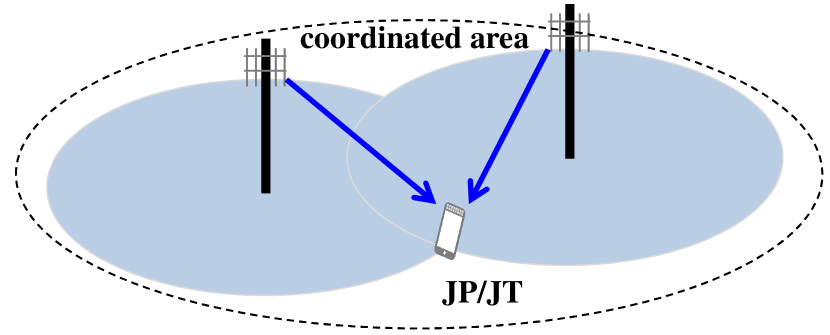
(a) Joint Processing/Joint Transmission (JP/JT): a MS is served simultaneously by two BSs.

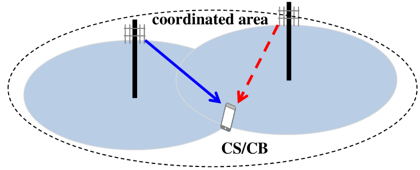
(b) Coordinated Scheduling/Coordinated Beamforming (CS/CB): a MS’s signal (solid blue arrow) is transmitted by one BS and the interference (red dashed arrow) coming from the other BS is coordinated.

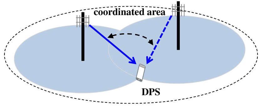
(c) Dynamic Point Selection (DPS): a MS is served by one single BS at any time and MS-BS association can be changed accordingly to the channel conditions.

Figure 1: Example operations of different CoMP modes.

In the JP/JT mode (Fig. 1(a)), the antennas of a cluster of coordinated BSs form a large single antenna array [5, 6]. The signals intended for a particular MS are simultaneously transmitted from multiple BSs across cell sites. Thus, JP/JT offers the benefit of large-scale BS cooperation [7, 8]. Asymptotic performance of JP/JT has been analyzed in recent works through the large system analysis of coordinated multicell systems [7, 8, 9]. Although JP/JT can exploit the best performance from the CoMP system, it is the most complex mode in terms of signaling and synchronization among the BSs [2]. Per the 3GPP LTE-Advanced Release 11, the JP/JT mode is normally assumed to be “coherent”, meaning that co-phasing of the signs from different coordinated transmission points is performed by means of precoding at the transmitter [2]. Thus, implementing JP/JT will need a high-resolution adjustable analog delay to each coordinated BS to cope with the delay variations. For this reason, it is difficult to fully realize the potential performance gains of coherent JP/JT, which may limit their applicability only to BSs connected by a fast backhaul [10, 11]. In addition, coherent JP/JT requires inter-point phase information as part of the channel state information (CSI) feedback from multiple points [12].

The CS/CB mode accounts for the least complex CoMP mode. In CS/CB (Fig. 1(b)), the signal to a single MS is transmitted from the serving cell only [2]. However, the beamforming functionality is dynamically coordinated between the BSs to control/reduce the ICI [2, 4, 13]. Optimal beamforming design for CoMP system under CS/CB mode can be obtained from joint optimization [13, 7, 8, 14, 15, 16, 17] or game theory [18]. To effectively coordinate the inter-cell interference, CS/CB requires CSI feedback from multiple points [12]. However, by exploiting channel reciprocality [12], optimal downlink CS/CB can be implemented if a BS knows the CSI only to its connected MSs [13].

In DPS mode (Fig. 1(c)), the MS, at any one time, is being associated to a single BS. However, this single associated BS can dynamically change from time-frame to time-frame within a set of possible BSs inside the cluster [2, 4, 19]. CoMP DPS provides a good trade-off between the transmission algorithm complexity, system performance and backhaul overhead, in comparison to JP/JT and CS/CB [20]. In fact, the synchronization issue and the requirement of fast backhaul communications can be alleviated in the DPS mode, compared to the JP/JT mode. In DPS, each MS’s data has to be available at all the possible BSs ready for selection. In addition, the beamforming functionality is still needed to coordinate the transmission across the BSs for interference control [2]. To facilitate the interference control, DPS demands similar CSI feedback as CS/CB such that no inter-point phase information is required [12]. In fact, when the user-BS association is determined, the DPS mode becomes the CS/CB mode. Compared to CS/CB, DPS offers the advantage of site selection diversity, since DPS can provide a “soft-handoff” solution to among the coordinated BSs to quickly switch the best BS for association for each MS. However, it is not clear how a joint BS association strategy and beamforming design in the DPS mode can be optimally determined to maximize the performance of the CoMP system. In this paper, we are interested in jointly optimizing the BS association strategy and linear beamforming design for a CoMP downlink system under the DPS mode. With a set of target signal-to-interference-plus-noise ratios (SINR) at the MSs, our design objective is to minimize either: i.) the weighted sum transmit power across the BSs or ii.) the per-BS transmit power margin.

I-A Related Works

Designing multicell beamformers under the CS/CB mode has attracted a lot of research attention, such as [13, 17, 7, 8, 14, 15, 16, 18]. Uplink-downlink duality and iterative fixed-point iteration have been successfully exploited in [13, 14, 15, 16, 17] to obtain optimal beamformers to either minimize the sum transmit power at the BSs or maximize the minimum SINR at the MSs. Different to these previous studies, part of this work examines the application of uplink-downlink duality to optimize the multicell beamformers under the DPS mode.

While the problem of joint BS association and beamforming design/power control in uplink transmission has been intensively studied [21, 22, 23], the counterpart problem in downlink transmission is not well understood. There are few prior studies in literature which deal with this downlink transmission problem. In [24], the problem for downlink transmission has been investigated for the case of power control (not including beamforming design). It is stated in [24] that there is no Pareto-optimal solution for the problem of joint BS association and beamforming design in the downlink. The work in [25] tackled the problem of joint downlink beamforming, power control, and access point allocation in a congested system. In [26], the joint optimization of BS association and beamforming design was examined and a relaxing-and-rounding technique was proposed as a suboptimal solution to the binary variables indicating the BS association. Recent works in [27, 28, 29] proposed joint BS association and power allocation/beamforming design strategies to maximize the multicell system throughput. In another work [30], the problem of joint BS assignment and power allocation for maximizing the minimum rate in a single-input single-output (SISO) interference channel was investigated. A two-stage algorithm was proposed to iteratively find the BS assignment and power allocation for the users [30]. In contrast to these works, our formulation and solution framework are to attain Pareto-optimal joint BS association and beamforming design strategies with guaranteed SINRs at the MSs.

In the context of finding the optimal beamforming design for power minimization, the optimization can be formulated as a nonconvex quadratic constrained quadratic programming (QCQP) problem [31]. The nonconvex QCQP is then solved indirectly via convex semi-definite programming (SDP) relaxation [31] or a transformation into a convex second-order conic programming (SOCP) problem [32, 33, 13]. It will be shown later in this paper that it is not possible to transform the problems under consideration into a SOCP. Thus, we rely on recent developments in nonconvex QCQP [34] in joinly devising the optimal BS association strategy and beamforming design.

I-B Contributions of This Paper

In this work, we formulate the joint BS association and beamforming design problems as mixed integer programs, which contain the binary variables indicating the BS associations. To circumvent the difficulty in dealing with the binary variables and devise optimal joint BS association and beamforming designs, our proposed solution approaches, which also account for the main contributions of this paper, are as follows:

• We propose a relaxation method to solve these original mixed integer programs by relaxing all the binary variables to $1$ and focusing on optimizing the beamformers. These relaxed optimization problems are shown to be nonconvex QCQP. Our analysis based the QCQP solution framework then shows that the relaxed problems can be solved optimally.

• Under the design objective of minimizing the weighted sum transmit power, the obtained solution from the relaxed problem is also optimal to the original problem. Specifically, this solution indicates both the optimal BS association strategy and the optimal beamforming design for all MSs. Our proposed framework also indicates that any Pareto-optimal solution can be obtained by properly adjusting the weight factors in the objective function of sum transmit power.

• We propose two solution approaches based on the Lagrangian duality and the dual uplink problem to find the optimal solution. Via the dual uplink problem, we propose a distributed algorithm to obtain the optimal joint BS association and beamforming design. We show that the DPS can be optimally implemented when a BS knows the CSI only to users within its serving user set.

• Under the design objective of minimizing the per-BS transmit power margin, the optimality of the relaxed problem’s solution to the original problem is not always observed. Nevertheless, based on the obtained solution from the relaxed problem, a suboptimal solution to the original problem is then proposed. We observe that the performance gap between the suboptimal solution to the optimal one is negligible in simulations. Simulation results also show that the resulting optimal joint BS association and beamforming design can significantly improve the performance of the CoMP system.

Notations: Superscripts $(\cdot)^{T}$, $(\cdot)^{*}$, $(\cdot)^{H}$ stand for transpose, complex conjugate, and complex conjugate transpose operations, respectively; upper-case bold face letters are used to denote matrices whereas lower-case bold face letters are used to denote column vectors; $\mathrm{diag}(d_{1},d_{2},\ldots,d_{M})$ denotes an $M\times M$ diagonal matrix with diagonal elements $d_{1},d_{2},\ldots,d_{M}$; $[\cdot]_{i,j}$ denotes the $(i,j)$ element of the matrix argument; $x^{\star}$ indicates the optimal value of the variable $x$; $\mathbf{A}\succeq\mathbf{B}$ (and $\mathbf{A}\succ\mathbf{B}$) is to indicate the matrix inequality (and strict matrix inequality) defined on the cone of nonnegative definite matrices; $\mathbf{A}\nsucc\mathbf{B}$ is to denote that $\mathbf{A}-\mathbf{B}$ is a semi-definite and singular matrix; $|x|$ denotes the absolute value of the scalar number $x$ whereas $|\mathcal{X}|$ denotes the cardinality of the set $\mathcal{X}$; $\mathbb{C}$ and $\mathbb{R}$ denote the sets of complex and real numbers, respectively.

II System Model and Problem Formulation

II-A System Model

We consider the multiuser downlink transmission in a multicell network consisting of $Q$ BSs and $K$ MSs operating on a same frequency band. Denote $\mathcal{Q}$ and $\mathcal{K}$ as the set of BSs and MSs, respectively. It is assumed that each BS is equipped with $M$ transmit antennas and each MS is equipped with a single receive antenna. In each cell, the BS multiplexes and concurrently sends multiple data streams to multiple MSs. However, each MS can be only associated with one BS at any time. In the downlink transmission to a particular MS, say MS-$i$, its received signal $y_{i}$ can be modeled as

$$y_{i}=\sum_{q=1}^{Q}\mathbf{h}_{iq}^{H}\mathbf{x}_{q}+z_{i},$$ (1)

where $\mathbf{x}_{q}\in\mathbb{C}^{M\times 1}$ is the transmitted signal at BS-$q$, $\mathbf{h}^{*}_{iq}\in\mathbb{C}^{M\times 1}$ represents the channel from BS-$q$ to MS-$i$, and $z_{i}$ is the AWGN with a power spectral density $\sigma^{2}$.

Let $\mathcal{Q}_{i}\subset\mathcal{Q}$ be the cluster of coordinated BSs serving user-$i$, and let $\mathcal{K}_{q}$ be the serving user set by BS-$q$. Let us define binary variables $a_{iq},i\in\mathcal{K},q\in\mathcal{Q}_{i}$ to represent the association between MS-$i$ and BS-$q$. More specifically, the binary variable $a_{iq}=1$ if and only if BS-$q\in\mathcal{Q}_{i}$ is assigned to serve MS-$i$. By means of linear beamforming, the transmitted signal at BS-$q$ can be formulated as

$$\mathbf{x}_{q}=\sum_{i\in\mathcal{K}_{q}}\mathbf{w}_{iq}u_{i},$$ (2)

where $\mathbf{w}_{iq}\in\mathbb{C}^{M\times 1}$ is the beamforming vector and $u_{i}$ is a complex scalar representing the signal intended for MS-$i$. Without loss of generality, let $\mathbb{E}[|u_{i}|]=1$. Clearly, if $a_{iq}=0$, $\mathbf{w}_{iq}$ needs to be set at all-$0$ vector. If BS-$q$ with $q\in\mathcal{Q}_{i}$ is selected to serve MS-$i$, the SINR at MS-$i$ is then given by

$$\mathrm{SINR}_{iq}=\frac{\big{|}\mathbf{h}_{iq}^{H}\mathbf{w}_{iq}\big{|}^{2}}{\sum\limits_{j\neq i}^{K}\sum\limits_{r\in\mathcal{Q}_{j}}\left|\mathbf{h}_{ir}^{H}\mathbf{w}_{jr}\right|^{2}+\sigma^{2}}.$$ (3)

II-B Problem Formulation

We first consider the joint BS association and beamforming design with the design objective of minimizing the weighted sum transmit power across the BSs with a set of target SINRs at the MSs. Let $w_{q}$ be the positive weight for the transmit power at BS-$q$. The optimization problem is then stated as

$$\mathcal{P}_{1}\,:\quad \underset{\{a_{iq}\},\{\mathbf{w}_{iq}\}}{\operatorname*{minimize}} \;\sum_{q=1}^{Q}w_{q}\sum_{i\in\mathcal{K}_{q}}\left\|\mathbf{w}_{iq}\right\|^{2}$$

$$\operatorname*{subject\;to} \;\sum_{q\in\mathcal{Q}_{i}}a_{iq}\mathrm{SINR}_{iq}\geq\gamma_{i},\forall i$$

$$\;a_{iq}=\{0,1\},\forall q\in\mathcal{Q}_{i},\forall i$$

$$\;\sum_{q\in\mathcal{Q}_{i}}a_{iq}=1,\forall i,$$

where the last constraint is to ensure that only one BS in $\mathcal{Q}_{i}$ will be associated with MS-$i$.

Remark 1: With a predetermined BS association strategy (known $a_{iq}$’s), problem $\mathcal{P}_{1}$ becomes the CS/CB design problem, whose optimal solution is readily obtainable [13]. In this case, the SINR constraints can be cast as convex second-order conic (SOC) constraints, which effectively transforms the optimization problem into a convex one. However, with the dynamic BS association strategy, the presence of binary variables $a_{iq}$, problem $\mathcal{P}_{1}$ is a nonconvex mixed integer program, which is NP-hard [35]. In fact, an exhaustive search for the optimal BS association has exponential complexity and is impractical for implementation.

One common method to solve a mixed integer program is relaxing the discrete variables into continuous ones [36]. In this work, we take a completely different approach by setting the binary variables $a_{iq}$’s to 1s. More precisely, we consider the following optimization problem:

$$\mathcal{P}^{\prime}_{1}\,:\quad \underset{\{\mathbf{w}_{iq}\}}{\operatorname*{minimize}} \;\sum_{q=1}^{Q}w_{q}\sum_{i\in\mathcal{K}_{q}}\left\|\mathbf{w}_{iq}\right\|^{2}$$

$$\operatorname*{subject\;to} \;\sum_{q\in\mathcal{Q}_{i}}\frac{\big{|}\mathbf{h}_{iq}^{H}\mathbf{w}_{iq}\big{|}^{2}}{\sum\limits_{j\neq i}^{K}\sum\limits_{r\in\mathcal{Q}_{j}}\left|\mathbf{h}_{ir}^{H}\mathbf{w}_{jr}\right|^{2}+\sigma^{2}}\geq\gamma_{i},\forall i.$$

Theorem 1.

The minimum weighted sum transmit power obtained from solving problem $\mathcal{P}^{\prime}_{1}$ is a lower-bound to that obtained from solving problem $\mathcal{P}_{1}$.

Proof:

Suppose that $(\{a_{iq}^{\star}\},\{\mathbf{w}_{iq}^{\star}\})$ is the optimal solution to the original joint BS and beamforming problem $\mathcal{P}_{1}$. From the solution $(a_{iq}^{\star},\mathbf{w}_{iq}^{\star})$, we denote $q_{i}\in\mathcal{Q}_{i}$ as the BS associated with MS-$i$. Since a MS can only be assigned to one BS, we have $a_{iq_{i}}^{\star}=1$, $a_{iq}^{\star}=0,\forall q\neq q_{i}$, and $\mathbf{w}_{iq_{i}}^{\star}\neq\mathbf{0}$ and $\mathbf{w}_{iq}^{\star}=\mathbf{0},\forall q\in\mathcal{Q}_{i},q\neq q_{i}$. In addition, $\{\mathbf{w}_{iq_{i}}^{\star}\}$ must be an optimal solution to the following problem

$$\bar{\mathcal{P}}_{1}\,:\quad \underset{\{\mathbf{w}_{iq_{i}}\}}{\operatorname*{minimize}} \;\sum_{i=1}^{K}w_{q_{i}}\left\|\mathbf{w}_{iq_{i}}\right\|^{2}$$

$$\operatorname*{subject\;to} \;\frac{\big{|}\mathbf{h}_{iq_{i}}^{H}\mathbf{w}_{iq_{i}}\big{|}^{2}}{\sum\limits_{j\neq i}^{K}\big{|}\mathbf{h}_{iq_{j}}^{H}\mathbf{w}_{jq_{j}}\big{|}^{2}+\sigma^{2}}\geq\gamma_{i},\forall i,$$

where $\big{|}\mathbf{h}_{iq_{j}}^{H}\mathbf{w}_{jq_{j}}\big{|}^{2}$ is the interference induced by the BS connected to MS-$j$, i.e., $q_{j}$, to MS-$i$. If additional constraints $\mathbf{w}_{iq}=\mathbf{0},\forall q\in\mathcal{Q}_{i},q\neq q_{i},\forall i$ are introduced to problem $\bar{\mathcal{P}}_{1}$, we will have the following optimization problem

$$\hat{\mathcal{P}}_{1}\,:\quad \underset{\{\mathbf{w}_{iq}\}}{\operatorname*{minimize}} \;\sum_{q=1}^{Q}w_{q}\sum_{i\in\mathcal{K}_{q}}\left\|\mathbf{w}_{iq}\right\|^{2}$$

$$\operatorname*{subject\;to} \;\frac{\sum_{q\in\mathcal{Q}_{i}}\big{|}\mathbf{h}_{iq}^{H}\mathbf{w}_{iq}\big{|}^{2}}{\sum\limits_{j\neq i}^{K}\sum\limits_{r\in\mathcal{Q}_{j}}\left|\mathbf{h}_{ir}^{H}\mathbf{w}_{jr}\right|^{2}+\sigma^{2}}\geq\gamma_{i},\forall i$$

$$\;\mathbf{w}_{iq}=\mathbf{0},\forall q\in\mathcal{Q}_{i},q\neq q_{i},\forall i.$$

Due to the additional constraints $\mathbf{w}_{iq}=\mathbf{0},\forall q\in\mathcal{Q}_{i},q\neq q_{i},\forall i$, the objective functions of problems $\bar{\mathcal{P}}_{1}$ and $\hat{\mathcal{P}}_{1}$ are the same. In addition, the numerators in the SINR constraints in the two problems are the same, so are the denominators. Thus, problem $\hat{\mathcal{P}}_{1}$ must yield the same solution as problem $\bar{\mathcal{P}}_{1}$, i.e., same optimal point. If the additional constraints $\mathbf{w}_{iq}=\mathbf{0},\forall q\in\mathcal{Q}_{i},q\neq q_{i},\forall i$ are now removed from problem $\hat{\mathcal{P}}_{1}$, we will have problem $\mathcal{P}_{1}^{\prime}$. Since problem $\mathcal{P}^{\prime}_{1}$ has a larger feasibility region than problem $\hat{\mathcal{P}}_{1}$, the minimum point of problem $\mathcal{P}^{\prime}_{1}$ must not exceed that of problem $\hat{\mathcal{P}}_{1}$. As a result, the optimal point of problem $\mathcal{P}^{\prime}_{1}$ is a lower bound to the optimal point of the original problem $\mathcal{P}_{1}$. ∎

Corollary 1.

If problem $\mathcal{P}_{1}$ is feasible, problem $\mathcal{P}^{\prime}_{1}$ is also feasible. Conversely, the infeasibility of problem $\mathcal{P}^{\prime}_{1}$ also indicates the infeasibility of problem $\mathcal{P}_{1}$.

Corollary 2.

Given that $\{\mathbf{w}_{iq}^{\star}\}$ with $i\in\mathcal{K},q\in\mathcal{Q}_{i}$ is the set of optimal beamformers obtained from solving problem $\mathcal{P}^{\prime}_{1}$, if there exists $q_{i}\in\mathcal{Q}_{i}$ such that $\mathbf{w}^{\star}_{iq_{i}}\neq\mathbf{0}$ and $\mathbf{w}^{\star}_{iq}=\mathbf{0},\forall q\neq q_{i}$, then $\{\mathbf{w}_{iq}^{\star}\}$ is also the optimal solution to problem $\mathcal{P}_{1}$.

Proof:

This corollary comes directly from Theorem 1 and its proof. The optimal BS association for MS-$i$ is then given by the BS index $q_{i}\in\mathcal{Q}_{i}$ corresponding to $\mathbf{w}^{\star}_{iq_{i}}\neq\mathbf{0}$. Moreover, $\mathbf{w}^{\star}_{iq_{i}}$ is also the optimal beamforming vector for MS-$i$. ∎

In the following sections, we focus on solving problem $\mathcal{P}^{\prime}_{1}$. It is noted the SINR constraint in problem $\mathcal{P}_{1}^{\prime}$ can be restated as

$$\sum_{q\in\mathcal{Q}_{i}}\big{|}\mathbf{h}_{iq}^{H}\mathbf{w}_{iq}\big{|}^{2}\geq\gamma_{i}\sum\limits_{j\neq i}^{K}\sum\limits_{r\in\mathcal{Q}_{j}}\big{|}\mathbf{h}_{ir}^{H}\mathbf{w}_{jr}\big{|}^{2}+\gamma_{i}\sigma^{2}.$$ (8)

If there is only one term on the left hand side of the above inequality constraint, say $\big{|}\mathbf{h}_{i{q}_{i}}^{H}\mathbf{w}_{i{q}_{i}}\big{|}^{2}$, one can assume $\mathbf{h}_{i{q}_{i}}^{H}\mathbf{w}_{i{q}_{i}}$ to be real. The constraint then can be transformed into a SOC form [32], which is convex. However, since we now have the summation of multiple terms $\sum_{q\in\mathcal{Q}_{i}}\big{|}\mathbf{h}_{iq}^{H}\mathbf{w}_{iq}\big{|}^{2}$, with $|\mathcal{Q}_{i}|>1$, there is no known method to transform the nonconvex quadratic constraint (8) into a convex form, e.g., SOC constraint. Thus, in order to devise an optimal solution to problem $\mathcal{P}_{1}^{\prime}$, we rely on the nonconvex QCQP framework presented in Section III. Interestingly, it will be shown the optimal solution to problem $\mathcal{P}^{\prime}_{1}$ indeed meets the conditions given in Corollary 2.

III Nonconvex Quadratic Constrained Quadratic Programming

This section presents a brief background on nonconvex QCQP and exposes relevant properties on strong duality of nonconvex QCQP. We consider a generic nonconvex QCQP as follows:

$$\mathcal{QCQP}\,:\quad \underset{\mathbf{x}\in\mathbb{C}^{N}}{\operatorname*{minimize}} \;f_{0}(\mathbf{x})$$

$$\operatorname*{subject\;to} \;f_{i}(\mathbf{x})\leq 0,\;i=1,\ldots,L,$$

where $f_{i}(\mathbf{x}),i=0,\ldots,L$ are quadratic, but not necessarily convex, functions on $\mathbf{x}\in\mathbb{C}^{N}$. The Lagrangian of problem (III) is given as

$$\mathcal{L}(\mathbf{x},\boldsymbol{\lambda})=f_{0}(\mathbf{x})+\sum_{i=1}^{L}\lambda_{i}f_{i}(\mathbf{x}),$$ (10)

where $\boldsymbol{\lambda}\triangleq[\lambda_{1},\ldots,\lambda_{L}]^{T}$ and $\lambda_{i}\geq 0$ is the Lagrangian multiplier associated with constraint $f_{i}(\mathbf{x})\leq 0,i=1,\ldots,L$. The dual function is then given by

$$g(\boldsymbol{\lambda})=\inf_{\mathbf{x}}\mathcal{L}(\mathbf{x},\boldsymbol{\lambda}).$$ (11)

By nature, the dual function $g(\boldsymbol{\lambda})$ is concave on $\boldsymbol{\lambda}\in\mathbb{R}^{L}_{+}$ [37]. Let $p^{\star}$ be the optimal value of problem $\mathcal{QCQP}$ and $d^{\star}$ be the optimal value of the dual problem $\operatorname*{maximize}_{\boldsymbol{\lambda}\geq 0}g(\boldsymbol{\lambda})$. By definition [37], one has

$$p^{\star}=\min_{\mathbf{x}}\;\sup_{\boldsymbol{\lambda}\geq\mathbf{0}}\mathcal{L}(\mathbf{x},\boldsymbol{\lambda}),$$ (12)

and $$d^{\star}=\max_{\boldsymbol{\lambda}\geq\mathbf{0}}\;\inf_{\mathbf{x}}\mathcal{L}(\mathbf{x},\boldsymbol{\lambda}).$$ (13)

Weak duality dictates that $d^{\star}\leq p^{\star}$ and the difference $p^{\star}-d^{\star}$ is called the duality gap (cf. Section 5 in [37]). If strong duality holds, i.e., zero duality gap with $d^{\star}=p^{\star}$, the optimal solution of the primal problem can be found through the dual problem as in (13). While strong duality holds for any convex optimization problem with Slater’s condition qualification, strong duality also obtains for nonconvex problems on rare occasions [37]. In any case of having strong duality, a saddle point $({\mathbf{x}}^{\star},{\boldsymbol{\lambda}}^{\star})$ for function $\mathcal{L}(\mathbf{x},\boldsymbol{\lambda})$, defined as

$$\mathcal{L}({\mathbf{x}}^{\star},\boldsymbol{\lambda})\!\leq\!\mathcal{L}({\mathbf{x}}^{\star},{\boldsymbol{\lambda}}^{\star})\!\leq\!\mathcal{L}(\mathbf{x},{\boldsymbol{\lambda}}^{\star}),\forall\mathbf{x}\in\mathbb{C}^{N},\forall\boldsymbol{\lambda}\in\mathbb{R}^{L}_{+},\;\;$$ (14)

must exist. The following property, presented in Section 5.4 of [37], underlines the connection between the existence of a saddle point for $\mathcal{L}(\mathbf{x},\boldsymbol{\lambda})$ and strong duality.

Property 1.

If the function $\mathcal{L}(\mathbf{x},\boldsymbol{\lambda})$ possesses a saddle point $({\mathbf{x}}^{\star},{\boldsymbol{\lambda}}^{\star})$ on $\mathbb{C}^{N}\times\mathbb{R}_{+}^{L}$, then strong duality $d^{\star}=p^{\star}$ holds. Conversely, if $d^{\star}$ is finite with ${\boldsymbol{\lambda}}^{\star}=\arg\max_{\boldsymbol{\lambda}\geq\mathbf{0}}g(\boldsymbol{\lambda})$, and the original problem has an optimal solution at ${\mathbf{x}}^{\star}$, then $({\mathbf{x}}^{\star},{\boldsymbol{\lambda}}^{\star})$ is a saddle point of $\mathcal{L}(\mathbf{x},\boldsymbol{\lambda})$.

The following property concerning the conditions on the existence of a saddle point has been presented in [34] and its proof was partially sketched in Page 1063 of the work.

Property 2.

The existence of a saddle point of $\mathcal{L}(\mathbf{x},\boldsymbol{\lambda})$ on $\mathbb{C}^{N}\times\mathbb{R}_{+}^{L}$ is equivalent to the following condition: there exists ${\boldsymbol{\lambda}}^{\star}$ such that the function $\mathcal{L}(\mathbf{x},{\boldsymbol{\lambda}}^{\star})$ is convex on $\mathbb{C}^{N}$ and has a minimizer ${\mathbf{x}}^{\star}$ on $\mathbb{C}^{N}$ satisfying ${\lambda}_{i}^{\star}f_{i}(\mathbf{x}^{\star})=0,f_{i}(\mathbf{x}^{\star})\leq 0,i=1,\ldots,L$.

Thus, in order to prove strong duality in a nonconvex QCQP problem and obtain its optimal solution via its Lagrangian dual problem, it suffices to show that the condition given in Property 2 is fulfilled [34]. Strong duality in nonconvex QCQP is also guaranteed under the following property, which is presented as Theorem 6 in [34].

Property 3.

Assume that the concave dual function $g(\boldsymbol{\lambda})=\inf_{\mathbf{x}}\mathcal{L}(\mathbf{x},\boldsymbol{\lambda})$ attains its maximum at a point $\boldsymbol{\lambda}^{\star}\in\mathbb{R}^{L}_{+}$. If $\mathcal{L}(\mathbf{x},\boldsymbol{\lambda}^{\star})$ is strictly convex on $\mathbb{C}^{N}$, then strong duality holds.

IV QCQP Solution Approach to Problem $\mathcal{P}^{\prime}_{1}$

This section presents an analytical approach to obtain an optimal solution to problem $\mathcal{P}^{\prime}_{1}$. It is noted that problem $\mathcal{P}^{\prime}_{1}$ is a nonconvex QCQP, which is NP-hard in general [34]. Our approach is to prove strong duality of this particular problem $\mathcal{P}^{\prime}_{1}$. First, the Lagrangian of problem $\mathcal{P}^{\prime}_{1}$ can be stated as

$$\mathcal{L}_{1}(\{\mathbf{w}_{iq}\},\boldsymbol{\lambda})$$

$$=\sum_{q=1}^{Q}w_{q}\sum_{i\in\mathcal{K}_{q}}\|\mathbf{w}_{iq}\|^{2}$$

$$\;\;-\sum_{i=1}^{K}\!\lambda_{i}\bigg{(}\frac{1}{\gamma_{i}}\!\!\sum_{q\in\mathcal{Q}_{i}}\!\big{|}\mathbf{h}_{iq}^{H}\mathbf{w}_{iq}\big{|}^{2}-\sum\limits_{j\neq i}^{K}\sum\limits_{r\in\mathcal{Q}_{j}}\left|\mathbf{h}_{ir}^{H}\mathbf{w}_{jr}\right|^{2}-\sigma^{2}\bigg{)}$$

$$=\sum_{i=1}^{K}\lambda_{i}\sigma^{2}$$

$$\;\;+\sum_{i=1}^{K}\!\sum_{q\in\mathcal{Q}_{i}}\!\mathbf{w}_{iq}^{H}\bigg{(}w_{q}\mathbf{I}\!-\!\frac{\lambda_{i}}{\gamma_{i}}\mathbf{h}_{iq}\mathbf{h}_{iq}^{H}\!+\!\sum_{j\neq i}^{K}\!\lambda_{j}\mathbf{h}_{jq}\mathbf{h}_{jq}^{H}\bigg{)}\mathbf{w}_{iq}.$$ (15)

The dual function is then given by $g_{1}(\boldsymbol{\lambda})=\min_{\{\mathbf{w}_{iq}\}}\mathcal{L}_{1}(\{\mathbf{w}_{iq}\},\boldsymbol{\lambda})$. Clearly, if any matrix $w_{q}\mathbf{I}-\frac{\lambda_{i}}{\gamma_{i}}\mathbf{h}_{iq}\mathbf{h}_{iq}^{H}\!+\!\sum_{j\neq i}^{K}\lambda_{j}\mathbf{h}_{jq}\mathbf{h}_{jq}^{H}$ is not positive semi-definite, it is possible to find $\mathbf{w}_{iq}$ to make $g_{1}(\boldsymbol{\lambda})$ unbounded below. Thus, the dual problem is given by

$$\underset{\boldsymbol{\lambda}\geq\mathbf{0}}{\operatorname*{maximize}} \;\sum_{i=1}^{K}\lambda_{i}\sigma^{2}$$

$$\operatorname*{subject\;to} \;w_{q}\mathbf{I}+\sum_{j\neq i}^{K}\lambda_{j}\mathbf{h}_{jq}\mathbf{h}_{jq}^{H}\succeq\frac{\lambda_{i}}{\gamma_{i}}\mathbf{h}_{iq}\mathbf{h}_{iq}^{H},\forall q\in\mathcal{Q}_{i},\forall i.$$

Remark 2: The dual problem is an SDP and a convex problem by nature. Its optimal solution can be easily obtained by the interior point method or standard SDP solvers, such as cvx [38]. However, a closer look on the dual problem (IV) can analytically establish an optimal solution to problem $\mathcal{P}^{\prime}_{1}$ as well as its feasibility. Note that the dual problem (IV) is always feasible (for instance, $\lambda_{i}=0,\forall i$ satisfies all the constraints). However, its feasibility does not necessarily indicate the feasibility of the primal problem $\mathcal{P}^{\prime}_{1}$. It may happen that $\lambda_{i}\rightarrow\infty$ at optimality and all constraints in (IV) are still satisfied, i.e., the dual problem is unbounded above. In this case, the primal problem $\mathcal{P}^{\prime}_{1}$ is infeasible thanks to the weak duality properties [37].

We now focus on the case where the optimal value of the dual problem (IV) is finite, i.e., the primal problem $\mathcal{P}^{\prime}_{1}$ is feasible.

Theorem 2.

If the nonconvex QCQP $\mathcal{P}^{\prime}_{1}$ is feasible, then strong duality holds.

Proof:

Denote $\boldsymbol{\lambda}^{\star}$ as the optimal solution of the dual problem. At $\boldsymbol{\lambda}^{\star}$, the function $\mathcal{L}_{1}(\{\mathbf{w}_{iq}\},\boldsymbol{\lambda}^{\star})$ is convex in $\{\mathbf{w}_{iq}\}$. Thus, in order to satisfy the conditions in Property 2 as presented in Section III, it is left to find $\{\mathbf{w}_{iq}^{\star}\}\in\arg\min_{\{\mathbf{w}_{iq}\}}\mathcal{L}(\{\mathbf{w}_{iq}\},\boldsymbol{\lambda}^{\star})$ such that $\{\mathbf{w}_{iq}^{\star}\}$ is feasible to problem $\mathcal{P}^{\prime}_{1}$ and moreover

$$\lambda_{i}^{\star}\!\!\left(\!\frac{1}{\gamma_{i}}\!\!\sum_{q\in\mathcal{Q}_{i}}\!\!\big{|}\mathbf{h}_{iq}^{H}\mathbf{w}_{iq}^{\star}\big{|}^{2}\ \!-\!\sum\limits_{j\neq i}^{K}\!\sum\limits_{r\in\mathcal{Q}_{j}}\!\!\left|\mathbf{h}_{ir}^{H}\mathbf{w}_{jr}^{\star}\right|^{2}\!-\!\sigma^{2}\!\right)\!\!=0,\forall i.$$ (17)

Consider the set of constraints related to MS-$i$ with optimal $\boldsymbol{\lambda}^{\star}$ in the dual problem (IV). Suppose that

$$w_{q}\mathbf{I}+\sum_{j\neq i}^{K}\lambda^{\star}_{j}\mathbf{h}_{jq}\mathbf{h}_{jq}^{H}\succ\frac{\lambda^{\star}_{i}}{\gamma_{i}}\mathbf{h}_{iq}\mathbf{h}_{iq}^{H},\forall q\in\mathcal{Q}_{i}.$$ (18)

We can increase $\lambda_{i}^{\star}$ to some value $\hat{\lambda}_{i}$ such that

$$w_{q}\mathbf{I}+\sum_{j\neq i}^{K}\lambda^{\star}_{j}\mathbf{h}_{jq}\mathbf{h}_{jq}^{H}\succeq\frac{\hat{\lambda}_{i}}{\gamma_{i}}\mathbf{h}_{iq}\mathbf{h}_{iq}^{H},\forall q\in\mathcal{Q}_{i}.$$ (19)

By setting $\hat{\lambda}_{j}=\lambda_{j}^{\star},\forall j\neq i$, one yields a feasible solution $\hat{\boldsymbol{\lambda}}=[\hat{\lambda}_{1},\ldots,\hat{\lambda}_{K}]^{T}$ that improves the objective function of problem (IV), i.e., $\sum_{i=1}^{K}\hat{\lambda}_{i}\sigma^{2}>\sum_{i=1}^{K}{\lambda}_{i}^{\star}\sigma^{2}$. Thus, $\boldsymbol{\lambda}^{\star}$ cannot be an optimal solution of problem $\eqref{dual-prob-2}$ by contradiction. As a result, there must exist a non-empty subset $\hat{\mathcal{Q}}_{i}\subset\mathcal{Q}_{i}$, such that

$$w_{q}\mathbf{I}+\sum_{j\neq i}^{K}\lambda_{j}^{\star}\mathbf{h}_{jq}\mathbf{h}_{jq}^{H}\nsucc\frac{\lambda_{i}^{\star}}{\gamma_{i}}\mathbf{h}_{iq}\mathbf{h}_{iq}^{H},\forall q\in\hat{\mathcal{Q}}_{i}.$$ (20)

Otherwise, $\lambda_{i}^{\star}$ can be further increased. Due to the above set of inequalities (with $\nsucc$), $\lambda_{i}^{\star},\forall i$ must be positive. For $q\in\mathcal{Q}_{i}\backslash\hat{\mathcal{Q}}_{i}$, strict inequality applies, i.e.,

$$w_{q}\mathbf{I}+\sum_{j\neq i}^{K}\lambda^{\star}_{j}\mathbf{h}_{jq}\mathbf{h}_{jq}^{H}\succ\frac{\lambda^{\star}_{i}}{\gamma_{i}}\mathbf{h}_{iq}\mathbf{h}_{iq}^{H},\forall q\in\mathcal{Q}_{i}\backslash\hat{\mathcal{Q}}_{i}.$$ (21)

Since strict inequality (21) is enforced $\forall q\in\mathcal{Q}_{i}\backslash\hat{\mathcal{Q}}_{i}$, the corresponding beamforming vector $\mathbf{w}^{\star}_{iq}$ must be set to all-$0$ vector in order to have the Lagrangian function (IV) minimized. On the other hand, since inequality (20) happens for $q\in\hat{\mathcal{Q}}_{i}$, there exists an eigenvector $\hat{\mathbf{w}}_{iq}\in\mathbb{C}^{M},\|\hat{\mathbf{w}}_{iq}\|=1$ corresponding to the $0$ eigenvalue, such that

$$\hat{\mathbf{w}}_{iq}^{H}\Bigg{(}\!w_{q}\mathbf{I}+\!\sum_{j\neq i}^{K}\lambda_{j}^{\star}\mathbf{h}_{jq}\mathbf{h}_{jq}^{H}\!-\frac{\lambda_{i}^{\star}}{\gamma_{i}}\mathbf{h}_{iq}\mathbf{h}_{iq}^{H}\Bigg{)}\hat{\mathbf{w}}_{iq}\!=0,\forall i,\forall q\in\hat{\mathcal{Q}}_{i}.$$ (22)

To minimize the Lagrangian $\mathcal{L}_{1}(\{\mathbf{w}_{iq}\},\boldsymbol{\lambda}^{\star})$, $\mathbf{w}_{iq}^{\star}$ can be chosen as a scaled version of $\hat{\mathbf{w}}_{iq}$. For each MS, say MS-$i$, a BS indexed as $q_{i}\in\hat{\mathcal{Q}}_{i}$ is randomly chosen and the corresponding beamforming vector $\mathbf{w}^{\star}_{iq_{i}}$ is set as $\sqrt{\delta_{i}}\hat{\mathbf{w}}_{iq_{i}}$, where the scaling coefficient $\delta_{i}>0$ will be determined shortly. For all BSs, $q\in\hat{\mathcal{Q}}_{i}$, $q\neq q_{i}$, $\mathbf{w}^{\star}_{iq}$ is purposely set at $\mathbf{0}$. Thus, we obtain a set of beamforming vector $\{\mathbf{w}_{iq}^{\star}\}_{\forall q\in\mathcal{Q}_{i}}\in\arg\min_{\{\mathbf{w}_{iq}\}}\mathcal{L}(\{\mathbf{w}_{iq}\},\boldsymbol{\lambda}^{\star})$. The next step is to determine $\delta_{i}$’s such that $\mathbf{w}^{\star}_{iq_{i}}$’s satisfies condition (17).

Note that $\lambda_{i}^{\star}>0,\forall i$ and $\mathbf{w}^{\star}_{iq}=\mathbf{0},\forall q\neq q_{i}$. By substituting $\mathbf{w}^{\star}_{iq_{i}}=\sqrt{\delta_{i}}\hat{\mathbf{w}}_{iq_{i}}$ into (17), we obtain a set of equations

$$\!\!\!\!\!\frac{\delta_{i}}{\gamma_{i}}\big{|}\mathbf{h}_{iq_{i}}^{H}\hat{\mathbf{w}}_{iq_{i}}\big{|}^{2}-\delta_{j}\sum\limits_{j\neq i}^{K}\big{|}\mathbf{h}_{iq_{j}}^{H}\hat{\mathbf{w}}_{jq_{j}}\big{|}^{2}=\sigma^{2},i=1,\ldots,K,$$ (23)

Equivalently, $\mathbf{G}\boldsymbol{\delta}=\mathbf{1}\sigma^{2}$, where $\boldsymbol{\delta}=[\delta_{1},\ldots,\delta_{K}]^{T}$ and $\mathbf{G}\in\mathbb{R}^{K\times K}$ is defined as $[\mathbf{G}]_{i,i}=(1/\gamma_{i})\big{|}\mathbf{h}_{iq_{i}}^{H}\hat{\mathbf{w}}_{iq_{i}}\big{|}^{2}$ and $[\mathbf{G}]_{i,j}=-\big{|}\mathbf{h}_{iq_{j}}^{H}\hat{\mathbf{w}}_{jq_{j}}\big{|}^{2}$.

It is noted that the set of equations in (22) can be cast as

$$\mathbf{G}^{T}\boldsymbol{\lambda}^{\star}=[w_{q_{1}},\ldots,w_{q_{K}}]^{T}>\mathbf{0}.$$ (24)

Since $\mathbf{G}^{T}$ is a $\mathbf{Z}$-matrix and there exists $\boldsymbol{\lambda}^{\star}>0$ such that $\mathbf{G}^{T}\boldsymbol{\lambda}^{\star}>\mathbf{0}$, $\mathbf{G}^{T}$ is an $\mathbf{M}$-matrix by its characterization (Condition I₂₈, Theorem 6.2.3 in [39]). Thus, $\mathbf{G}$, also an $\mathbf{M}$-matrix, is invertible and its inverse is a positive matrix [39]. As a result, $\boldsymbol{\delta}>\mathbf{0}$ can be determined by

$$\boldsymbol{\delta}=\mathbf{G}^{-1}\mathbf{1}\sigma^{2}.$$ (25)

Since $\{\mathbf{w}_{iq_{i}}^{\star}=\sqrt{\delta_{i}}\hat{\mathbf{w}}_{iq_{i}}\}_{\forall i}$ now satisfies the set of equations (22), we yield a feasible solution to the problem $\mathcal{P}_{1}^{\prime}$ where each constraint is met with equality. The qualification of condition (17) by $\{\mathbf{w}_{iq_{i}}^{\star}\}$ then guarantees the satisfaction of all conditions in Property 2. Strong duality for problem $\mathcal{P}_{1}^{\prime}$ then follows. Furthermore, $\{\mathbf{w}_{iq_{i}}^{\star}\}$ must be a globally optimal solution of the nonconvex problem $\mathcal{P}^{\prime}_{1}$. ∎

We now relate the optimal solution $\{\mathbf{w}_{iq_{i}}^{\star}\}$ of problem $\mathcal{P}_{1}^{\prime}$ to the original mixed-integer problem $\mathcal{P}_{1}$ as follows.

Proposition 1.

The obtained optimal solution $\{\mathbf{w}_{iq_{i}}^{\star}\}$ of problem $\mathcal{P}_{1}^{\prime}$ is also optimal to the original mixed-integer problem $\mathcal{P}_{1}$. Furthermore, $q_{i}$ indicates an optimal BS association for MS-$i$.

Proof:

In solving problem $\mathcal{P}_{1}^{\prime}$, we derived an optimal solution where $\mathbf{w}_{iq_{i}}^{\star}\neq\mathbf{0}$ and $\mathbf{w}_{iq}^{\star}=\mathbf{0},\forall q\neq q_{i}$. Thus, Corollary 2 is applicable. The optimality of $\{\mathbf{w}_{iq_{i}}^{\star}\}$ to problem $\mathcal{P}_{1}$ and the association of MS-$i$ to BS-$q_{i}$ follow. ∎

Through numerous numerical simulations, we observe that inequality (20) is met at only one BS in the set $\mathcal{Q}_{i}$, i.e., $|\hat{\mathcal{Q}}_{i}|=1$, except for the extremely rare cases where the channels from two BSs are exactly symmetric or two BSs are co-located. We address the cases when $|\hat{\mathcal{Q}}_{i}|>1$ in the following proposition.

Proposition 2.

If $|\hat{\mathcal{Q}}_{i}|>1$, MS-$i$ can be associated to either one of the BSs in the set $\mathcal{\hat{Q}}_{i}$ without affecting minimum weighted sum transmit power across the BSs.

Proof:

If $|\hat{\mathcal{Q}}_{i}|>1$, we can first select any BS, say $q_{i}\in\hat{\mathcal{Q}}_{i}$, such that the corresponding beamformer $\mathbf{w}_{q_{i}}^{\star}$ is set to be non-zero and $\mathbf{w}_{q}^{\star}=\mathbf{0},\forall q\neq q_{i}$. The derivation steps (22)–(25) can be sequentially applied to determine the scaling factor and the beamformers $\{\mathbf{w}_{iq}^{\star}\}$ for all the users. Interestingly, different association schemes (with $q_{i}\in\mathcal{\hat{Q}}_{i}$ and their corresponding beamforming designs) might yield different globally optimal solutions to problem $\mathcal{P}_{1}^{\prime}$ with the same optimal value. The reason for this result is because the obtained solutions $(\mathbf{w}_{iq}^{\star},\boldsymbol{\lambda}^{\star})$ will satisfy the set of equations (17) and other conditions in Property 2 to be globally optimal. In addition, different BS assignments for MS-$i$ in $\hat{\mathcal{Q}}_{i}$ will also yield the same minimum weighted sum power across the BSs, which must equal to the optimal value of the dual problem (IV), $\sum_{i=1}^{K}\lambda_{i}^{\star}\sigma^{2}$. In spite of that, individual transmit powers at the BSs might not be the same with different BS assignments for MS-$i$. ∎

Since the $\mathcal{P}_{1}$ can be optimally solved, any Pareto-optimal solution of the problem can be obtained by properly adjusting the weight factor $w_{q}$’s in the objective function.

V Interpretation via Uplink-Downlink Duality

In the previous section, we have presented an analytical approach to solve problem $\mathcal{P}^{\prime}_{1}$ via its Lagrangian dual problem. In this section, we provide an alternative approach for solving problem $\mathcal{P}^{\prime}_{1}$ via the well-known uplink-downlink duality. It will be shown shortly that the Lagrangian dual problem (IV) is indeed the power minimization problem with SINR constraints in the uplink. We note that uplink-downlink duality is a powerful tool which has been studied in different contexts of multicell beamforming designs [13, 14, 15, 16, 17]. Fixed-point iterative algorithms were proposed to find the corresponding optimal beamforming solutions [13, 14, 15, 16]. Herein, we show that uplink-downlink duality is also applicable to the joint BS association and beamforming design problem under consideration. We then propose an iterative fixed-point algorithm to effectively solve the problem.

V-A Dual Uplink System Model

We consider the dual uplink system with the same setting as in Section II. Specifically, the dual uplink system is derived from the downlink system by transposing the channel matrices and by interchanging the input and the output vectors. In addition, the noise at each BS, say BS-$q$, is assumed to be zero mean AWGN with the covariance matrix $\sigma^{2}w_{q}\mathbf{I}$. Herein, the single-antenna MS-$q$ is transmitting at power $\hat{p}_{i}$ and $\mathbf{h}_{iq}$ is the uplink channel from MS-$i$ to BS-$q$. If MS-$i$ is associated with BS-$q$ where $q\in\mathcal{Q}_{i}$, the BS then applies the receive beamforming vector $\hat{\mathbf{w}}_{iq}$ to decode MS-$i$’s signal. In the considered uplink system, the BS association is performed by selecting a BS in $\mathcal{Q}_{i}$ such that MS-$i$ needs to transmit at minimum power to obtain the SINR target $\gamma_{i}$ at the very BS. Thus, the design objective now is to jointly optimize the power allocation $\hat{p}_{i}$’s, the receive beamforming vector $\hat{\mathbf{w}}_{iq},q\in\mathcal{Q}_{i},\forall i$, and the BS association to satisfy the set of SINR constraints $\gamma_{i}$’s. The joint uplink optimization can be stated as

$$\underset{\hat{p}_{1},\ldots,\hat{p}_{K},\{\hat{\mathbf{w}}_{iq}\}}{\operatorname*{minimize}} \!\sum_{i=1}^{K}\hat{p}_{i}$$

$$\operatorname*{subject\;to} \!\max_{q\in\mathcal{Q}_{i}}\frac{\hat{p}_{i}\big{|}\hat{\mathbf{w}}_{iq}^{H}\mathbf{h}_{iq}\big{|}^{2}}{\sum\limits_{j\neq i}^{K}\hat{p}_{j}\big{|}\hat{\mathbf{w}}_{iq}^{H}\mathbf{h}_{jq}\big{|}^{2}+\sigma^{2}w_{q}\hat{\mathbf{w}}_{iq}^{H}\hat{\mathbf{w}}_{iq}}\geq\gamma_{i},\forall i.$$

We now underline the connection between the downlink problem $\mathcal{P}^{\prime}_{1}$ and the dual uplink problem (V-A).

Proposition 3.

The optimal downlink beamforming problem $\mathcal{P}^{\prime}_{1}$ can be solved via a dual uplink problem in which the SINR constraints remain the same. Specifically, the Lagrangian dual problem (IV) of problem $\mathcal{P}^{\prime}_{1}$ is the following problem

$$\underset{\lambda_{1},\ldots,\lambda_{K},\{\hat{\mathbf{w}}_{iq}\}}{\operatorname*{minimize}} \!\sum_{i=1}^{K}\lambda_{i}\sigma^{2}$$

$$\operatorname*{subject\;to} \!\max_{q\in\mathcal{Q}_{i}}\frac{\lambda_{i}\sigma^{2}\big{|}\hat{\mathbf{w}}_{iq}^{H}\mathbf{h}_{iq}\big{|}^{2}}{\sum\limits_{j\neq i}^{K}\!\lambda_{j}\sigma^{2}\big{|}\hat{\mathbf{w}}_{iq}^{H}\mathbf{h}_{jq}\big{|}^{2}\!+\sigma^{2}w_{q}\hat{\mathbf{w}}_{iq}^{H}\hat{\mathbf{w}}_{iq}}\!\geq\!\gamma_{i},\forall i,$$

where $\hat{p}_{i}=\lambda_{i}\sigma^{2}$ is dual uplink power of MS-$i$. If the dual uplink problem (3) is feasible, its optimal solution is also optimal to the Lagrangian dual problem (IV). Otherwise, the Lagrangian dual problem (IV) is unbounded above.

Proof:

For given uplink power allocation $\hat{p}_{i}=\lambda_{i}\sigma^{2}$, the optimal receive beamforming vector at BS-$q,q\in\mathcal{Q}_{i}$ is the minimum mean-squared error (MMSE) receiver

$$\hat{\mathbf{w}}_{iq}=\Bigg{(}\sum_{j=1}^{K}\lambda_{j}\mathbf{h}_{jq}\mathbf{h}_{jq}^{H}+w_{q}\mathbf{I}\Bigg{)}^{-1}\mathbf{h}_{iq}.$$ (28)

By substituting the above MMSE receiver $\hat{\mathbf{w}}_{iq}$, the SINR constraint for MS-$i$ in (3) becomes

$$\!\!\lambda_{i}\!\left(\!1+\frac{1}{\gamma_{i}}\right)\!\cdot\max_{q\in\mathcal{Q}_{i}}\mathbf{h}_{iq}^{H}\Bigg{(}\sum_{j=1}^{K}\lambda_{j}\mathbf{h}_{jq}\mathbf{h}_{jq}^{H}+w_{q}\mathbf{I}\!\Bigg{)}^{-1}\!\!\mathbf{h}_{iq}\geq 1.\!\!$$ (29)

Note that the above set of constraints for $i=1,\ldots,K$ may constitute an empty set, which then renders the dual uplink problem infeasible. However, if the dual uplink problem (3) is feasible, at optimality the set of inequality constraints (29) must meet at equality, i.e.,

$$\!\!\lambda_{i}\!\left(\!1\!+\frac{1}{\gamma_{i}}\right)\!\cdot\max_{q\in\mathcal{Q}_{i}}\mathbf{h}_{iq}^{H}\Bigg{(}\sum_{j=1}^{K}\lambda_{j}\mathbf{h}_{jq}\mathbf{h}_{jq}^{H}+w_{q}\mathbf{I}\!\Bigg{)}^{-1}\!\!\mathbf{h}_{iq}=1,\forall i.$$ (30)

Thanks to Lemma 1 in [33] as provided following this proof, the constraint in the Lagrangian dual problem (IV) can be recast as

$$\!\lambda_{i}\left(\!1\!+\!\frac{1}{\gamma_{i}}\right)\mathbf{h}_{iq}^{H}\Bigg{(}\!\sum_{j=1}^{K}\lambda_{j}\mathbf{h}_{jq}\mathbf{h}_{jq}^{H}+w_{q}\mathbf{I}\!\Bigg{)}^{-1}\!\!\mathbf{h}_{iq}\leq 1,\forall q\in\mathcal{Q}_{i},$$

or equivalently,

$$\lambda_{i}\!\left(\!1+\frac{1}{\gamma_{i}}\right)\!\cdot\max_{q\in\mathcal{Q}_{i}}\mathbf{h}_{iq}^{H}\Bigg{(}\sum_{j=1}^{K}\lambda_{j}\mathbf{h}_{jq}\mathbf{h}_{jq}^{H}+w_{q}\mathbf{I}\!\Bigg{)}^{-1}\!\!\mathbf{h}_{iq}\leq 1.$$ (31)

Unlike the dual uplink problem (3), the Lagrangian dual problem (IV) is always feasible, thanks to its nonempty constraint set. In case of having a finite optimal value, it is clear that at optimality the set of inequality constraints (31) must be met at equality, as given in (30). Thus, the power minimization problem (3) of $\sum_{i=1}^{K}\lambda_{i}\sigma^{2}$ with minimum SINR constraints (29) and the power maximization problem (IV) of $\sum_{i=1}^{K}\lambda_{i}\sigma^{2}$ with maximum SINR constraints in (31) are equivalent since $\lambda_{i}$’s in both problems are the fixed point of the equations (30). It will be shown shortly that this fixed point is unique if it exists. In that case, the fixed point is the optimal solution for both problems. If a fixed point does not exist, the dual uplink problem (3) is not feasible and equivalently the Lagrangian dual problem (IV) is unbounded above. ∎

For completeness, Lemma 1 in [33] is presented as follows: “Let $\mathbf{A}$ be an $n\times n$ symmetric positive semidefinite matrix and $\mathbf{b}$ be an $n\times 1$ vector. Then, $\mathbf{A}\succeq\mathbf{b}\mathbf{b}^{H}$ if and only if $\mathbf{b}^{H}\mathbf{A}^{-1}\mathbf{b}\leq 1$.”

V-B An Iterative Algorithm for Solving Problem $\mathcal{P}^{\prime}_{1}$

Having established the equivalence between the Lagrangian dual problem (IV) and the dual uplink problem (3), this section focuses on obtaining the solution to both problems by finding the fixed point to the set of equations (30). By rearranging (30) into a fixed point iteration, one has

$$\lambda_{i}^{(n+1)} = \min_{q\in\mathcal{Q}_{i}}f_{iq}\big{(}\boldsymbol{\lambda}^{(n)}\big{)},$$ (32)

where $f_{iq}(\boldsymbol{\lambda})$ is defined as

$$f_{iq}(\boldsymbol{\lambda})=\frac{\gamma_{i}}{1+\gamma_{i}}\cdot\frac{1}{\mathbf{h}_{iq}^{H}\mathbf{\Sigma}_{q}^{-1}\!\mathbf{h}_{iq}}.$$ (33)

and $\mathbf{\Sigma}_{q}=\!\sum_{j=1}^{K}\lambda_{j}\mathbf{h}_{jq}\mathbf{h}_{jq}^{H}+w_{q}\mathbf{I}$.

Proposition 4.

If a fixed point of (30) exists, it is unique and the iterative function evaluation (32) converges geometrically fast to the fixed point.

Proof:

It is proven in [32, 33] that $f_{iq}(\boldsymbol{\lambda})$ satisfies the three properties (positivity, monotonicity, and scalability) to be a standard function. Moreover, the point-wise minimum of a set of standard function, i.e., $\min_{q\in\mathcal{Q}_{i}}f_{iq}(\boldsymbol{\lambda})$, is also a standard function [41]. Thus, the iteration (32) converges geometrically fast to the fixed point, if it exists. ∎

The iteration (32) accounts for the first step of the iterative algorithm to solve problem $\mathcal{P}_{1}^{\prime}$. The second step is to find the optimal receive beamformer $\hat{\mathbf{w}}_{iq_{i}}$, where $q_{i}$ is the BS association with MS-$i$. Then, the final step is to obtain the optimal transmit beamformer ${\mathbf{w}}_{iq_{i}}$. We summarize these three steps in the following Algorithm 1.

1Initialize $\lambda_{i}>0$, $\forall i$;

2 repeat

3      Update $\lambda_{i}$ as given in equation (32),

4      until convergence to $\boldsymbol{\lambda}^{\star}$;

5     Set $q_{i}=\arg\min_{q\in\mathcal{Q}_{i}}f_{iq}(\boldsymbol{\lambda}^{\star}),\forall i$;

6      Find the receive beamformer $\hat{\mathbf{w}}_{q_{i}}$ as given in equation (28);

7      Find the transmit beamformer $\mathbf{w}_{iq_{i}}^{\star}=\sqrt{\delta_{i}}\hat{\mathbf{w}}_{q_{i}}$, where $\delta_{i}$ is given by (25);

Algorithm 1 Iterative Algorithm for Minimizing The Weighted Sum Transmit Power

V-C Distributed Implementation

An interesting development from the above uplink-downlink duality interpretation is that all the three steps in the iterative algorithm proposed in the previous section can be implemented distributively. Herein, it is assumed that the system is operating in the time division duplex (TDD) mode where the uplink and downlink channels are reciprocal. It is also assumed that the weight $w_{q}$ is known at BS-$q$.

In the first step, the iteration (32) on the uplink power $\lambda_{i}$ involves only its channel vectors $\mathbf{h}_{iq}$’s and the matrices $\mathbf{\Sigma}_{q}$’s obtained from the BSs in $\mathcal{Q}_{i}$. With known $w_{q}$, BS-$q$ can compensate the background noise to $w_{q}\sigma^{2}$. Then $\mathbf{\Sigma}_{q}$, as the covariance matrix of the total received signal at BS-$q$ in the uplink, can be estimated locally by the BS. Thus, the transmit powers $\lambda_{i}$’s can be updated as in (32) on a per-user basis without inter-BS or inter-user coordination. Should the acquisition of the channel $\mathbf{h}_{iq}$’s or the matrices $\mathbf{\Sigma}_{q}$’s be challenging at the MSs, BS-$q$ can simply calculate $f_{iq}=\frac{\gamma_{i}}{1+\gamma_{i}}\cdot\frac{1}{\mathbf{h}_{iq}^{H}\mathbf{\Sigma}_{q}^{-1}\!\mathbf{h}_{iq}}$ for $i\in\mathcal{K}_{q}$ as the required transmit power at MS-$i$ to obtain its target SINR $\gamma_{i}$ at the very BS. Subsequently, $f_{iq}$’s are passed to MS-$i$, who will choose the lowest uplink power $\lambda_{i}=\min_{q\in\mathcal{Q}_{i}}f_{iq}$. The BS that can achieve the SINR $\gamma_{i}$ with the uplink power $\lambda_{i}$ is then the one associated with MS-$i$. Thanks to Proposition 4, these iterative steps always converge to a fixed point if it exists.

While the second step to determine the MMSE receivers (28) is straightforward at the BSs, the final step to calculate the scaling factors $\delta_{i}$’s is more involved. In particular, although $\delta_{i}$’s are found as in (25), this matrix inversion process requires centralized implementation. On the other hand, finding $\delta_{i}$’s is equivalent to the downlink power control problem for achieving a set target SINRs $\gamma_{i}$’s. One solution approach is the Foschini-Miljanic’s algorithm where the optimal downlink powers can be found iteratively in a fully distributed manner using per-user power updates [42].

Remark 3: In downlink CS/CB, it is shown in [13] that the optimal downlink beamforming can be obtained even if each BS only knows the CSI to its connected MSs by exploiting channel reciprocality. Via the distributed implementation presented in this section, we show that the optimal BS association and beamforming design in the DPS mode can be devised if each BS only knows the CSI to the MSs in its serving user set, i.e., BS-$q$ needs the CSI $\mathbf{h}_{iq}$ to the MSs in $\mathcal{K}_{q}$. By exploiting channel reciprocality, BS-$q$ can listen to the training signal from MS-$i$ in the uplink transmission for estimating $\mathbf{h}_{iq}$. The only signaling or feedback involved is passing of the required transmit power $f_{iq}$ for MS-$i$ to connect to BS-$q$ in the uplink. MS-$i$ is then required to make the recommendation of its selected BS $q_{i}$, i.e., $q_{i}=\arg\min_{q\in\mathcal{Q}_{i}}f_{iq}$. This selection recommendation by the MSs is consistent with the CoMP implementation in the LTE Release 11 [12].

VI Semidefinite Programming Relaxation

In this section, we present the SDP relaxation approach to find an optimal solution to problem $\mathcal{P}^{\prime}_{1}$. It is well known that SDP relaxation can be successfully exploited to find the optimal multiuser beamforming design for single-cell systems [31, 32, 43]. To apply the SDP relaxation to the multicell system model under consideration, we first replace $\mathbf{w}_{iq}\mathbf{w}_{iq}^{H}$ by $\mathbf{X}_{iq}$ and $\mathbf{h}_{iq}\mathbf{h}_{iq}^{H}$ by $\mathbf{H}_{iq}$ and recast problem $\mathcal{P}^{\prime}_{1}$ into an SDP

$$\underset{\{\mathbf{X}_{iq}\}}{\operatorname*{minimize}} \!\sum_{q=1}^{Q}w_{q}\sum_{i\in\mathcal{K}_{q}}\mathrm{Tr}\{\mathbf{X}_{iq}\}$$

$$\operatorname*{subject\;to} \!\frac{1}{\gamma_{i}}\!\!\sum_{q\in\mathcal{Q}_{i}}\!\!\mathrm{Tr}\{\mathbf{H}_{iq}\mathbf{X}_{iq}\}\!-\!\sum\limits_{j\neq i}^{K}\!\sum\limits_{r\in\mathcal{Q}_{j}}\!\!\mathrm{Tr}\{\mathbf{H}_{ir}\mathbf{X}_{jr}\!\}\!\geq\!\sigma^{2},\forall i$$

$$\mathbf{X}_{iq}\succeq\mathbf{0},\;\mathrm{rank}\{\mathbf{X}_{iq}\}=1.$$

Since the rank constraint is nonconvex, we remove it and relax problem (VI) into a convex SDP. Once we have a convex SDP, the interior-point method can be applied to find its optimal solution. Through numerous numerical simulations, we found a similar result reported [31, 43] that a rank-$1$ solution of the SDP relaxation problem can always be found. Thus, it is possible to retrieve $\mathbf{w}_{iq}$ from the obtained solution in $\mathbf{X}_{iq}$. In addition, it is even more interesting that among the optimal solution set related to a particular MS, e.g., $\{\mathbf{X}_{iq}\},q\in\mathcal{Q}_{i}$, there is only one non-zero (and rank-$1$) matrix. As a result, solving the SDP relaxation version of problem (VI) provides the optimal solution not only to the beamforming problem $\mathcal{P}^{\prime}_{1}$, but also to the original joint BS association and beamforming design problem $\mathcal{P}_{1}$.

It is noted that the obtained optimal result from the SDP relaxation approach can be proved analytically. First, it can be shown that the Lagrangian dual of the SDP relaxation version of problem (VI) is the same as problem (IV). Second, problem (IV) is the dual problem of the QCQP $\mathcal{P}_{1}^{\prime}$ and strong duality holds. Thus, our proposed framework via nonconvex QCQP in Section IV provides a rigorous analytical confirmation to the numerical results obtained here by the SDP relaxation approach. Nonetheless, the drawback of the SDP relaxation approach is the complexity in solving the relaxed version of problem (VI) due to the expanded set of variables. Certainly, solving the convex SDP in the Lagrangian dual problem (IV) is much simpler.

VII Minimization of The Per-Base-Station Transmit Power Margin

In the optimization problem $\mathcal{P}_{1}$, the adjustment of the weight factors $w_{q}$’s provides a trade-off among the power consumptions at different BSs. In this section, we consider a practical scenario of minimizing the transmit power margin across the BSs, in which the weights are implicitly determined. To jointly optimize the BS association and the beamforming design, the optimization problem can be formulated as follows:

$$\mathcal{P}_{2}\,:\quad \underset{\{a_{iq}\},\{\mathbf{w}_{iq}\},\alpha}{\operatorname*{minimize}} \;\alpha\sum_{q=1}^{Q}P_{q}$$

$$\operatorname*{subject\;to} \;\sum_{q\in\mathcal{Q}_{i}}a_{iq}\mathrm{SINR}_{iq}\geq\gamma_{i},\forall i$$

$$\;a_{iq}=\{0,1\},\forall q\in\mathcal{Q}_{i},\forall i$$

$$\;\sum_{q\in\mathcal{Q}_{i}}a_{iq}=1,\forall i,$$

$$\;\sum_{i\in\mathcal{K}_{q}}\left\|\mathbf{w}_{iq}\right\|^{2}\leq\alpha P_{q}.$$

Herein, $\alpha$ represents the margin between the transmit power of a BS, say BS-$q$, and its maximum power value $P_{q}$. By minimizing $\alpha$, the multicell system tries to balance the power consumptions across the BSs and does not overuse any of them. This formulation is especially beneficial to heterogeneous multicell systems where $P_{q}$’s can be different by one or two orders of magnitude. The resulting optimal $\alpha^{\star}$ from problem $\mathcal{P}_{2}$ is also important to verify the compliance of individual power constraints at the BSs. Specifically, if $\alpha^{\star}\leq 1$, then it is feasible to find an optimal BS association and beamforming design to meet all the SINR constraints and the per-BS power constraint $\sum_{i\in\mathcal{{K}}_{q}}\|\mathbf{w}_{iq}\|^{2}\leq P_{q},\forall q$.

Similar to problem $\mathcal{P}_{1}$, problem $\mathcal{P}_{2}$ is a difficult nonconvex mixed integer program. Thus, we take a similar approach in solving problem $\mathcal{P}_{1}$ by relaxing problem $\mathcal{P}_{2}$ into the following optimization problem:

$$\mathcal{P}_{2}^{\prime}\,:\quad \underset{\{\mathbf{w}_{iq}\},\alpha}{\operatorname*{minimize}} \;\alpha\sum_{q=1}^{Q}P_{q}$$

$$\operatorname*{subject\;to} \;\sum_{q\in\mathcal{Q}_{i}}\frac{\big{|}\mathbf{h}_{iq}^{H}\mathbf{w}_{iq}\big{|}^{2}}{\sum\limits_{j\neq i}^{K}\sum\limits_{r\in\mathcal{Q}_{j}}\left|\mathbf{h}_{ir}^{H}\mathbf{w}_{jr}\right|^{2}+\sigma^{2}}\geq\gamma_{i},\forall i$$

$$\;\sum_{i\in\mathcal{K}_{q}}\left\|\mathbf{w}_{iq}\right\|^{2}\leq\alpha P_{q}.$$

In other words, we let all the binary variables $a_{iq}$ to be $1$. Let us denote $\alpha^{\star}$ and $\alpha^{-}$ as the optimal solutions in problems $\mathcal{P}_{2}$ and $\mathcal{P}_{2}^{\prime}$, respectively.

Remark 4: Theorem 1 is also applicable to the relaxation of problem $\mathcal{P}_{2}$ into problem $\mathcal{P}_{2}^{\prime}$. Corollary 2 is also applicable to the optimal solution of problem $\mathcal{P}_{2}^{\prime}$. Unfortunately, solving problem $\mathcal{P}_{2}^{\prime}$ does not always provide us a solution that meets the conditions in Corollary 2. To illustrate this observation, let us consider a simple system setting with $K=1$ and $Q=2$. In solving problem $\mathcal{P}_{1}^{\prime}$, the MS will be assigned to the BS that requires the lowest transmit power. However, under the problem formulation $\mathcal{P}_{2}^{\prime}$, the obtained solution will result in non-zero transmit powers at both BSs to have $\alpha$ minimized, i.e., the transmit powers are split and balanced at the both BSs. Nevertheless, in solving problem $\mathcal{P}_{2}^{\prime}$, one can obtain the lower bound on the optimal value of problem $\mathcal{P}_{2}$.

Remark 5: Suppose that one has obtained $\{\mathbf{w}_{iq}^{-}\}$ as the optimal solution to problem $\mathcal{P}_{2}^{\prime}$. Let $q_{i}^{+}=\arg\max_{q\in\mathcal{Q}_{i}}\\ \mathrm{SINR}_{iq}=\arg\max_{q\in\mathcal{Q}_{i}}\big{|}\mathbf{h}_{iq}^{H}\mathbf{w}_{iq}^{-}\big{|}^{2}$ be the BS association with MS-$i$. Then, for a known BS association profile $\{q_{i}^{+}\},i=1,\ldots,K$, an optimal beamforming design for minimizing the transmit power margin across the BSs can be easily found [44] by solving the following optimization

$$\underset{\{\mathbf{w}_{iq_{i}}\},\alpha}{\operatorname*{minimize}} \;\alpha\sum_{q=1}^{Q}P_{q}$$

$$\operatorname*{subject\;to} \;\frac{\big{|}\mathbf{h}_{iq_{i}}^{H}\mathbf{w}_{iq_{i}}\big{|}^{2}}{\sum_{j\neq i}^{K}\big{|}\mathbf{h}_{iq_{j}}^{H}\mathbf{w}_{jq_{j}}\big{|}^{2}+\sigma^{2}}\geq\gamma_{i},\forall i$$

$$\;\sum_{i\in\mathcal{K}_{q},q_{i}=q}\left\|\mathbf{w}_{iq_{i}}\right\|^{2}\leq\alpha P_{q}.$$

We denote the obtained per-BS transmit power margin as $\alpha^{+}$. Certainly, $\alpha^{-}$ and $\alpha^{+}$ serve as a lower bound and an upper bound on $\alpha^{\star}$, i.e.,

$$\alpha^{-}\leq\alpha^{\star}\leq\alpha^{+}.$$ (38)

We observe through numerous simulations that the gap between $\alpha^{-}$ and $\alpha^{+}$ is nonexistent for most of the simulations (with $K>1$). For these cases, solving problem $\mathcal{P}_{2}^{\prime}$ does provide the optimal solution of problem $\mathcal{P}_{2}$ too. For other cases, the BS association profile $\{q_{i}\},i=1,\ldots,K$ and its corresponding beamforming design can be employed as a suboptimal solution to problem $\mathcal{P}_{2}$.

VII-A QCQP Solution Approach to Problem $\mathcal{P}_{2}^{\prime}$

In this section, we apply the QCQP solution approach presented in Section IV to devise the globally optimal solution to problem $\mathcal{P}_{2}^{\prime}$. The Lagrangian of problem $\mathcal{P}_{2}^{\prime}$ can be stated as

$$\mathcal{L}_{2}(\{\mathbf{w}_{iq}\},\alpha,\boldsymbol{\lambda},\boldsymbol{\mu})$$

$$=\alpha\sum_{q=1}^{Q}P_{q}+\sum_{q=1}^{Q}\mu_{q}\bigg{(}\sum_{i\in\mathcal{K}_{q}}\left\|\mathbf{w}_{iq}\right\|^{2}-\alpha P_{q}\bigg{)}$$

$$\;\;-\sum_{i=1}^{K}\!\lambda_{i}\bigg{(}\frac{1}{\gamma_{i}}\!\!\sum_{q\in\mathcal{Q}_{i}}\!\big{|}\mathbf{h}_{iq}^{H}\mathbf{w}_{iq}\big{|}^{2}-\sum\limits_{j\neq i}^{K}\sum\limits_{r\in\mathcal{Q}_{j}}\left|\mathbf{h}_{ir}^{H}\mathbf{w}_{jr}\right|^{2}-\sigma^{2}\bigg{)}$$

$$=\sum_{i=1}^{K}\lambda_{i}\sigma^{2}+\alpha\bigg{(}\sum_{q=1}^{Q}P_{q}-\sum_{q=1}^{Q}\mu_{q}P_{q}\bigg{)}$$

$$\;\;+\sum_{i=1}^{K}\!\sum_{q\in\mathcal{Q}_{i}}\mathbf{w}_{iq}^{H}\bigg{(}\mu_{q}\mathbf{I}-\frac{\lambda_{i}}{\gamma_{i}}\mathbf{h}_{iq}\mathbf{h}_{iq}^{H}\!+\!\sum_{j\neq i}^{K}\!\lambda_{j}\mathbf{h}_{jq}\mathbf{h}_{jq}^{H}\bigg{)}\mathbf{w}_{iq},$$ (39)

where $\lambda_{i}$’s and $\mu_{q}$’s are the Lagrangian multipliers associated with the SINR and the power constraints and $\boldsymbol{\lambda}\triangleq[\lambda_{1},\ldots,\lambda_{K}]^{T}$ and $\boldsymbol{\mu}\triangleq[\mu_{1},\ldots,\mu_{Q}]^{T}$. The dual function is then given by $g_{2}(\boldsymbol{\lambda},\boldsymbol{\mu})=\min_{\{\mathbf{w}_{iq}\},\alpha}\mathcal{L}_{2}(\{\mathbf{w}_{iq}\},\alpha,\boldsymbol{\lambda},\boldsymbol{\mu})$. If any matrix $\mu_{q}\mathbf{I}-\frac{\lambda_{i}}{\gamma_{i}}\mathbf{h}_{iq}\mathbf{h}_{iq}^{H}\!+\!\sum_{j\neq i}^{K}\!\lambda_{j}\mathbf{h}_{jq}\mathbf{h}_{jq}^{H}$ is not positive semi-definite or $\sum_{q=1}^{Q}P_{q}<\sum_{q=}^{Q}\mu_{q}P_{q}$, it is possible to find $\mathbf{w}_{iq}$ or $\alpha>0$ to make $g_{2}(\boldsymbol{\lambda},\boldsymbol{\mu})$ unbounded below. Thus, the dual problem is defined as

$$\underset{\boldsymbol{\lambda}\geq\mathbf{0},\boldsymbol{\mu}\geq\mathbf{0}}{\operatorname*{maximize}} \;\sum_{i=1}^{K}\lambda_{i}\sigma^{2}$$

$$\operatorname*{subject\;to} \;\mu_{q}\mathbf{I}+\sum_{j\neq i}^{K}\lambda_{j}\mathbf{h}_{jq}\mathbf{h}_{jq}^{H}\succeq\frac{\lambda_{i}}{\gamma_{i}}\mathbf{h}_{iq}\mathbf{h}_{iq}^{H},\forall q\in\mathcal{Q}_{i},\forall i$$

$$\;\sum_{q=1}^{Q}\mu_{q}P_{q}\leq\sum_{q=1}^{Q}P_{q}.$$

Compared to problem (IV) with pre-determined weight factors $w_{q}$’s, the variable $\mu_{q}$, functioning as the weight for the transmit power at BS-$q$, have to be optimized in problem (VII-A). Since the dual problem (VII-A) is convex, its optimal solution can be efficiently obtained by standard convex optimization techniques.

Let $\boldsymbol{\lambda}^{\star}$ and $\boldsymbol{\mu}^{\star}$ be the optimal solution of problem (VII-A). Except an extremely rare case where the channels from the BSs to the MSs are exactly symmetric, it is not possible to have $\mu_{q}^{\star}\mathbf{I}+\sum_{j\neq_{i}}^{K}\lambda_{j}^{\star}\mathbf{h}_{jq}\mathbf{h}_{jq}^{H}\nsucc\frac{\lambda_{i}^{\star}}{\gamma_{i}}\mathbf{h}_{iq}\mathbf{h}_{iq}^{H},\;\forall q\in\mathcal{Q}_{i},\forall i$. Thus, $\mathcal{L}_{2}(\{\mathbf{w}_{iq}\},\alpha,\boldsymbol{\lambda}^{\star},\boldsymbol{\mu}^{\star})$ is a strictly convex function. According to Property 3 in Section III, strong duality holds, i.e., the optimal solution of problem $\mathcal{P}_{2}^{\prime}$, can be found through the dual problem (VII-A). It is noted that $\mathbf{w}_{iq}^{-}$ must be set to $\mathbf{0}$ to have the Lagrangian function (VII-A) minimized should $\mu_{q}^{\star}\mathbf{I}+\sum_{j\neq_{i}}^{K}\lambda_{j}^{\star}\mathbf{h}_{jq}\mathbf{h}_{jq}^{H}\succ\frac{\lambda_{i}^{\star}}{\gamma_{i}}\mathbf{h}_{iq}\mathbf{h}_{iq}^{H}$. By applying the same argument as in the proof of Theorem 2, the optimal solution $\{\mathbf{w}_{iq}^{-}\}$ to problem $\mathcal{P}_{2}^{\prime}$ typically has a sparse structure.

In one special case, among the set of constraints related to a MS, say MS-$i$, if there exists only one $q_{i}\in\mathcal{Q}_{i}$ such that

$$\mu_{q_{i}}^{\star}\mathbf{I}+\sum_{j\neq_{i}}^{K}\lambda_{j}^{\star}\mathbf{h}_{jq_{i}}\mathbf{h}_{jq_{i}}^{H}\nsucc\frac{\lambda_{i}^{\star}}{\gamma_{i}}\mathbf{h}_{iq_{i}}\mathbf{h}_{iq_{i}}^{H},$$ (41)

and

$$\mu_{q}^{\star}\mathbf{I}+\sum_{j\neq}^{K}\lambda_{j}^{\star}\mathbf{h}_{jq}\mathbf{h}_{jq}^{H}\succ\frac{\lambda_{i}^{\star}}{\gamma_{i}}\mathbf{h}_{iq}\mathbf{h}_{iq}^{H},\;\forall q\in\mathcal{Q}_{i},q\neq q_{i},$$ (42)

then one has $\mathbf{w}_{iq_{i}}^{-}\neq\mathbf{0}$ and $\mathbf{w}_{iq}^{-}=\mathbf{0},\forall q\neq q_{i},\forall i$ as the optimal solution to problem $\mathcal{P}_{2}^{\prime}$. Since the requirements in Corollary 2 are now satisfied, the optimal solution of problem $\mathcal{P}_{2}$ is also found. In other cases, the steps given in Remark 5 can be applied to generate a suboptimal BS association and beamforming design solution of problem $\mathcal{P}_{2}$. We summarize the steps to obtain lower and upper bounds on the optimal per-BS transmit power margin $\alpha^{\star}$ and a suboptimal solution of problem $\mathcal{P}_{2}$ in Algorithm 2.

1Solve the dual problem (VII-A) to obtain the optimal dual solutions $\boldsymbol{\lambda}^{\star}$ and $\boldsymbol{\mu}^{\star}$;

2 Obtain the optimal primal solution $\{\mathbf{w}_{iq_{i}}^{-}\}$, $\alpha^{-}$ of problem $\mathcal{P}_{2}^{\prime}$;

3 Set $\alpha^{-}$ as the lower bound on $\alpha^{\star}$;

4 Verify if conditions (41)–(42) are satisfied;

5 if yes;

6  then $\{\mathbf{w}_{iq_{i}}^{-}\}$ is optimal to problem $\mathcal{P}_{2}$;

7 otherwise set $q_{i}=\arg\max_{q\in\mathcal{Q}_{i}}\big{|}\mathbf{h}_{iq}^{H}\mathbf{w}_{iq_{i}}^{-}\big{|}^{2}$;

8 Set $\{q_{i}\}$ as a suboptimal BS association strategy;

9 Solve problem (VII) to obtain the upper bound $\alpha^{+}$ on $\alpha^{\star}$ and the corresponding beamforming design;

Algorithm 2 Iterative Algorithm for Minimizing The Per-BS Transmit Power Margin

VII-B A Comparison to the Relaxation-and-Rounding Techniques in [26]

In a prior work [26], we proposed two relaxation-and-rounding techniques to solve the joint BS association and beamforming design problem $\mathcal{P}_{2}$. Of the two techniques, the better performing ‘relaxation-based-2’ approach first relaxes all BS association variables $\{a_{iq}\}$ to $1$ and finds the beamforming design through the optimization

$$\tilde{\mathcal{P}}_{2}:\quad \underset{\{\mathbf{w}_{iq}\},\alpha}{\operatorname*{minimize}} \;\alpha\sum_{q=1}^{Q}P_{q}$$

$$\operatorname*{subject\;to} \;\frac{\bigg{|}\sum\limits_{q\in\mathcal{Q}_{i}}\mathbf{h}_{iq}^{H}\mathbf{w}_{iq}\bigg{|}^{2}}{\sum\limits_{j\neq i}^{K}\bigg{|}\sum\limits_{r\in\mathcal{Q}_{j}}\mathbf{h}_{ir}^{H}\mathbf{w}_{jr}\bigg{|}^{2}+\sigma^{2}}\geq\gamma_{i},\forall i$$

$$\;\sum_{i\in\mathcal{K}_{q}}\left\|\mathbf{w}_{iq}\right\|^{2}\leq\alpha P_{q}.$$

The obtained solution, denoted as $\{\tilde{\mathbf{w}}_{iq}\}$, is then utilized for generating a BS association profile in a similar fashion as given in Remark 5. Subsequently, the beamforming design can be found accordingly to the generated BS association profile [26].

It is noted that there is a subtle difference between problems $\mathcal{P}_{2}^{\prime}$ and $\tilde{\mathcal{P}}_{2}$ in expressing the SINR constraints. In fact, with the SINR constraint expression in (VII-B), problem $\tilde{\mathcal{P}}_{2}$ mimics the optimization of the beamformers in a single-cell system with power constraints per groups of antennas. It is noted that problem $\tilde{\mathcal{P}}_{2}$ can be recast into a convex second-order conic program (SOCP) [26]. A quick verification on the dual problem of the optimization $\tilde{\mathcal{P}}_{2}$ would indicate that the obtained optimal solution $\{\tilde{\mathbf{w}}_{iq}\}$ does not have a sparse structure, i.e., $\tilde{\mathbf{w}}_{iq}\neq\mathbf{0},\,\forall i,\forall q$. Hence, $\{\tilde{\mathbf{w}}_{iq}\}$ cannot be an optimal solution of the original problem $\mathcal{P}_{2}$, unlike the solution $\{\mathbf{w}_{iq}^{-}\}$ obtained from solving problem $\mathcal{P}_{2}^{\prime}$. In addition, the obtained optimal value from solving problem (VII-B), denoted as $\tilde{\alpha}$, is typically much smaller than the one from solving problem $\mathcal{P}_{2}^{\prime}$, i.e., $\alpha^{-}$. Thus, the relaxation-and-rounding approach in [26] usually generates a large gap between the lower bound and upper bound on $\alpha^{\star}$, unlike the proposed QCQP solution approach proposed in this work. A numerical comparison between the two approaches will be presented in the simulation to verify this observation.

VII-C SDP Relaxation

In order to obtain a globally optimal solution to the optimization problem $\mathcal{P}_{2}^{\prime}$, we can also apply the SDP approach. Let $\mathbf{X}_{iq}=\mathbf{w}_{iq}\mathbf{w}_{iq}^{H}$ and $\mathbf{H}_{iq}=\mathbf{h}_{iq}\mathbf{h}_{iq}^{H}$, the QCQP $\mathcal{P}_{2}^{\prime}$ can be recast as an SDP

$$\underset{\{\mathbf{X}_{iq}\},\alpha}{\operatorname*{minimize}} \alpha\sum_{q=1}^{Q}P_{q}$$

$$\operatorname*{subject\;to} \frac{1}{\gamma_{i}}\!\!\sum_{q\in\mathcal{Q}_{i}}\!\!\mathrm{Tr}\{\mathbf{H}_{iq}\mathbf{X}_{iq}\}\!-\!\sum\limits_{j\neq i}^{K}\!\sum\limits_{r\in\mathcal{Q}_{j}}\!\!\mathrm{Tr}\{\mathbf{H}_{ir}\mathbf{X}_{jr}\!\}\!\geq\!\sigma^{2},\forall i$$

$$\sum_{i\in\mathcal{K}_{q}}\mathrm{Tr}\{\mathbf{X}_{iq}\}\leq\alpha P_{q}$$

$$\mathbf{X}_{iq}\succeq\mathbf{0}.$$

Herein, the rank constraint $\mathrm{rank}\{\mathbf{X}_{iq}\}=1$ is dropped to render problem (VII-C) as a convex SDP. This convex relaxation SDP then can be optimally solved by the interior-point method and a convex SDP solver like cvx [38].

Since strong duality holds for the QCQP $\mathcal{P}_{2}^{\prime}$ and the dual problem of the SDP (VII-C) is also (VII-A), a rank-$1$ solution of $\{\mathbf{X}_{iq}\},\forall q,\forall i$ can always be found. Should the obtained solution of problem (VII-C) meet all the requirements in Corollary 2, it is also the optimal solution to the joint optimization of BS association and beamforming design problem $\mathcal{P}_{2}$. Otherwise, the approximation steps in Remark 5 can be applied to generate a suboptimal solution of problem $\mathcal{P}_{2}$.

VIII Numerical Results

This section presents the numerical evaluations on the power consumption of a multiuser multicell system employing dynamic BS association. In all simulations, we assume that the locations of the BSs are fixed and the distance between any two nearby BSs is normalized to $1$, whereas the MSs are randomly located. Each BS is equipped with $M=4$ transmit antennas. The channel from a BS to a MS is generated from i.i.d. Gaussian random variables (Rayleigh fading) using the path loss model with the path loss exponent of $4$ and the reference distance of $1$. The transmit power at each BS is limited at $1$ W ($0$ dB). The AWGN power spectral density $\sigma^{2}$ is assumed to be $0.01$ W while the target SINRs at the MSs are set the same $\gamma$.

In the first simulation setting, we consider a two-cell system with $4$ randomly located MSs between the two BSs. The target SINR $\gamma$ is set at $16$ dB. For a randomly generated channel realization, we plot in Fig. 2 the Pareto-optimal tradeoff curve in the transmit powers at the two BSs employing dynamic BS association. To obtain each tradeoff point, we vary $w_{1}$ in the interval $[0,1]$ and set $w_{2}=1-w_{1}$. Depending on the weights, our proposed framework can obtain the corresponding Pareto-optimal joint BS association and beamforming design. In fact, it is impossible to find a joint BS association and beamforming design that results in a power allocation profile below the plotted Pareto-optimal tradeoff curve. Note that at the extreme points of the tradeoff curves, the MSs are all assigned to either one of the two BSs.

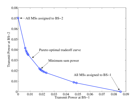
Figure 2: The Pareto-optimal tradeoff curve in power consumption between the two BSs with optimal joint BS association and beamforming design.

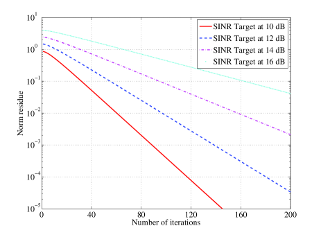
Figure 3: Convergence of the proposed iterative algorithm to solve Problem $\mathcal{P}_{1}^{\prime}$ with different SINR targets. The speed of convergence is slower with higher SINR targets.

Fig. 3 illustrates the convergence of the iterative algorithm in Section V-B, which allows us to obtain the optimal solution to problem $\mathcal{P}_{1}^{\prime}$. In the figure, we plot the norm residue $\|\boldsymbol{\lambda}^{(n)}-\boldsymbol{\lambda}^{\star}\|$ (where $\boldsymbol{\lambda}^{\star}$ is the optimal uplink power vector) versus the number of iterations with different SINR targets. It is observed that the fixed-point iteration (32) converges very fast. Interestingly, the speed of convergence becomes slower with increasing SINR targets.

In the second simulation setting, we compare the results obtained from the optimal BS association (with different clustering sizes) to that obtained from fixed BS association schemes. Examples of fixed BS association schemes for a MS are the channel-based scheme (assigned to the BS with the strongest downlink channel) and the location-based scheme (assigned to the closest BS). With fixed BS association, the beamforming vectors for the MSs and the transmit power at the BSs are optimally obtained by means of coordinated beamforming [13]. We consider a multicell system with $7$ BSs (each equipped with four antennas) and $10$ MSs, as illustrated in Fig. 4. Of the $7$ cells, we consider two clustering scenarios: i.) universal clustering with all $7$ cells and ii.) $3$-cell clustering with cluster #1 (cell #1, #2, and #3), cluster #2 (cell #1, #4, and #5), and cluster #3 (cell #1, #6, and #7). In the $3$-cell clustering scenario, a MS, say MS-$i$, is first assigned to a cluster based on its relative distance to the center of the cluster. MS-$i$ then can only be associated to one of the $3$ BSs within its assigned cluster.

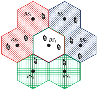
Figure 4: A seven-cell network grouped into three clusters with ten randomly located MSs. A MS can only be associated to one of the BSs in its assigned cluster.

Fig. 5 displays the percentage of finding a feasible beamforming strategy to meet the target SINR at the MSs with different BS association schemes. As the target SINR varies, $10,000$ channel realizations at each SINR value are used to obtain the ratios in Fig. 6. Unlike the first simulation setting with $M=K=4$, it is not always possible to find a feasible beamforming strategy in the second simulation setting where $M=4$ and $K=10$. It is observed from the figure that the chance of finding a feasible beamformer design can be doubled by the proposed DPS strategy, thanks to the optimal and dynamic association of the MSs to the BSs. In contrast, by pre-determining the associations, an optimal CS/CB strategy using [13] may not be found at high probability. Interestingly, by grouping the cells into clusters of $3$ cells, one can obtain nearly the same optimal performance achieved by the larger cluster of $7$ cells.

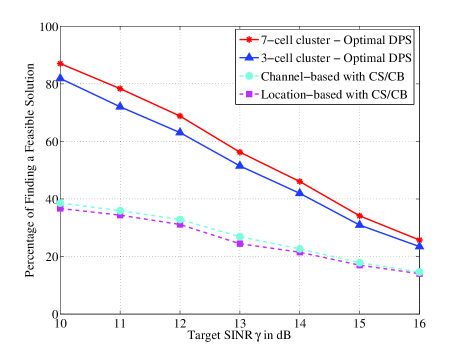
Figure 5: Percentage of finding a beamforming design to meet the target SINR with different BS association schemes. The optimal DPS can double the chance of finding a feasible solution, compared to the fixed BS association schemes with optimal CS/CB [13].

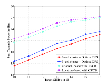
Figure 6: Average sum transmit power versus target SINR with different BS association schemes. The optimal DPS can save more than $5$ dB in the sum transmit power, compared to the fixed BS association schemes with optimal CS/CB [13].

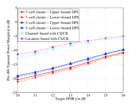
Figure 7: Per-BS transmit power margin versus target SINR with different BS association schemes. The optimal DPS can provide a much better balance in transmit powers across the BSs and reduce the peak transmit power as much as $7$ dB, compared to the fixed BS association schemes with optimal CS/CB [13].

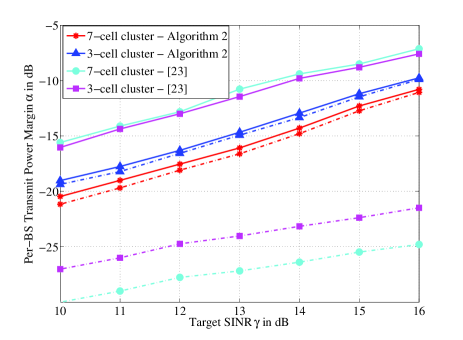
Figure 8: Comparing the per-BS transmit power margins obtained from Algorithm 2 and the approach in [26]: solid lines are for the upper bounds and dashed-dotted lines are for the lower bounds. The proposed DPS scheme in Algorithm 2 provides a much smaller gap between its upper bound and lower bound, compared to the approach in [26].

Fig. 6 illustrates the average sum transmit power across the $7$ BSs (with equal weights) versus the target SINR at the MSs (each MS is set at the same SINR target). As observed from the figure, more transmit power is required to meet the higher target SINR. Out of the considered BS association schemes, it is clearly shown that the optimal joint BS association and beamforming design significantly outperforms the fixed BS association schemes (location-based and channel-based). In particular, the optimal joint schemes can save the transmit power at each BS up to $5$ dB over the fixed BS association schemes with optimal CS/CB [13]. It is also observed that the optimal joint scheme with 3-cell clustering only imposes a penalty of $0.5$ dB in power usage, compared to the full 7-cell clustering. Clearly, a small cluster size is much more beneficial for practical implementation.

Fig. 7 shows the performance of the joint BS association and beamforming design for minimizing per-BS transmit power margin. As observed from the figure, the per-BS transmit power margin is reduced by at least $5$ dB to $10$ dB by the dynamic BS association schemes proposed in Algorithm 2, compared to the fixed BS association schemes with optimal CS/CB in [13]. Herein, the lower bound was generated by solving problem $\mathcal{P}_{2}^{\prime}$, whereas the upper bound was generated by the BS association profile $\{q_{i}^{+}\}$ accordingly to the solution of problem $\mathcal{P}_{2}^{\prime}$. It is also observed from the figure that the gap between the two bounds on the transmit power margin as given in (38) is very tight for both $3$-cell and $7$-cell clustering schemes. Hence, the proposed joint BS association and beamforming design in Algorithm 2 can generate an exceptionally well-performed and near-optimal solution to the original problem $\mathcal{P}_{2}$.

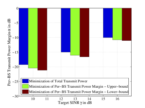
Figure 9: Comparing the per-BS transmit power margin with $3$-cell clustering for the sum power minimization and the per-BS transmit power margin minimization. The latter design criterion can reduce the peak transmit power by $1$-$2$ dB, compared to the former one.

In Fig. 8, we compare the performance between the proposed Algorithm 2 in this work and the prior work in [26]. As observed from the figure, by relying on the solution of problem $\tilde{\mathcal{P}}_{2}$, the approach in [26] generates a very large gap between the lower bound and upper bound on the optimal value of problem $\mathcal{P}_{2}$. In contrast, the tight gap generated by Algorithm 2 allows us to determine the minimum per-BS transmit power margin more properly. In addition, coupled with a closer upper bound, Algorithm 2 also generates a better suboptimal BS association and beamforming design than the approach in [26].

Finally, Fig. 9 compares the per-BS transmit power margins with $3$-cell clustering obtained from the two design objectives: sum power minimization and per-BS power margin minimization. It is observed from the figure that the per-BS power margin can be reduced around $1$-$2$ dB by the latter design criterion.

IX Conclusion

This paper has presented a solution framework to obtain an optimal joint BS association and beamforming design for downlink transmission. The design objective was to minimize either the weighted transmit power across the BSs or the per-BS transmit power margin with a set of target SINRs at the MSs. By properly relaxing the nonconvex joint BS association and beamforming design problems, we have shown that their optimal solutions can be obtained via the relaxed problems. Under the first design objective, such optimality is always guaranteed. Two solution approaches based on the Lagrangian duality and the dual uplink problem have been then proposed to find an optimal solution. Under the second design objective, based on the obtained solution from the relaxed problem, a near-optimal solution to the original problem is then proposed. Simulation results have shown the superior performance of the optimal joint BS association and beamforming design over fixed BS association schemes. In addition, simulation shows that $3$-cell clustering is sufficient to obtain a very close performance to the universal clustering.

References

- [1] D. H. N. Nguyen, L. B. Le, and T. Le-Ngoc, “Optimal joint base station association and beamforming design for downlink transmission,” in Proc. IEEE Int. Conf. Commun., London, UK, Jun. 2015, pp. 4966–4971.
- [2] 4G Americas, 4G Mobile Broadband Evolution: 3GPP Release 11 & Release 12 and Beyond, Feb. 2014.
- [3] D. H. N. Nguyen and T. Le-Ngoc, Wireless Coordinated Multicell Systems: Architectures and Precoding Designs, ser. SpringerBriefs in Computer Science. Springer, 2014.
- [4] H.-L. Määttänen, K. Hämäläinen, J. Venäläinen, K. Schober, M. Enescu, and M. Valkama, “System-level performance of LTE-advanced with joint transmission and dynamic point selection schemes,” EURASIP J. Adv. Signal Process., vol. 2012, no. 1, pp. 1–18, 2012.
- [5] M. Karakayali, G. Foschini, and R. Valenzuela, “Network coordination for spectrally efficient communications in cellular systems,” IEEE Wireless Commun., vol. 13, no. 4, pp. 56–61, Aug. 2006.
- [6] D. Gesbert, S. Hanly, H. Huang, S. S. Shitz, O. Simeone, and W. Yu, “Multi-cell MIMO cooperative networks: a new look at interference,” IEEE J. Select. Areas in Commun., vol. 28, no. 9, pp. 1380–1408, Dec. 2010.
- [7] R. Zakhour and S. V. Hanly, “Base station cooperation on the downlink: Large system analysis,” IEEE Trans. Inform. Theory, vol. 58, no. 4, pp. 2079–2106, Apr. 2012.
- [8] L. Sanguinetti, R. Couillet, and M. Debbah, “Large system analysis of base station cooperation for power minimization,” IEEE Trans. Wireless Commun., vol. 15, no. 8, pp. 5480–5496, Aug. 2016.
- [9] J. Zhang, C. K. Wen, S. Jin, X. Gao, and K. K. Wong, “Large system analysis of cooperative multi-cell downlink transmission via regularized channel inversion with imperfect CSIT,” IEEE Trans. Wireless Commun., vol. 12, no. 10, pp. 4801–4813, Oct. 2013.
- [10] D. Lee, H. Seo, B. Clerckx, E. Hardouin, D. Mazzarese, S. Nagata, and K. Sayana, “Coordinated multipoint transmission and reception in LTE-advanced: deployment scenarios and operational challenges,” IEEE Commun. Mag., vol. 50, no. 2, pp. 148–155, Feb. 2012.
- [11] J. Lee, Y. Kim, H. Lee, B. L. Ng, D. Mazzarese, J. Liu, W. Xiao, and Y. Zhou, “Coordinated multipoint transmission and reception in LTE-Advanced systems,” IEEE Commun. Mag., vol. 50, no. 11, pp. 44–50, Nov. 2012.
- [12] 3GPP Technical Report TR36.819, Coordinated multi-point operation for LTE physical layer aspects. 3rd Generation Partnership Project, 2012.
- [13] H. Dahrouj and W. Yu, “Coordinated beamforming for the multicell multi-antenna wireless system,” IEEE Trans. Wireless Commun., vol. 9, no. 5, pp. 1748–1759, May 2010.
- [14] Y. Huang, G. Zheng, M. Bengtsson, K. K. Wong, L. Yang, and B. Ottersten, “Distributed multicell beamforming with limited intercell coordination,” IEEE Trans. Signal Process., vol. 59, no. 2, pp. 728–738, Feb. 2011.
- [15] S. He, Y. Huang, L. Yang, A. Nallanathan, and P. Liu, “A multi-cell beamforming design by uplink-downlink max-min SINR duality,” IEEE Trans. Wireless Commun., vol. 11, no. 8, pp. 2858–2867, 2012.
- [16] Y. Huang, G. Zheng, M. Bengtsson, K. K. Wong, L. Yang, and B. Ottersten, “Distributed multicell beamforming design approaching pareto boundary with max-min fairness,” IEEE Trans. Wireless Commun., vol. 11, no. 8, pp. 2921–2933, Aug. 2012.
- [17] Y. Huang, C. W. Tan, and B. D. Rao, “Joint beamforming and power control in coordinated multicell: Max-min duality, effective network and large system transition,” IEEE Trans. Wireless Commun., vol. 12, no. 6, pp. 2730–2742, Jun. 2013.
- [18] D. H. N. Nguyen and T. Le-Ngoc, “Multiuser downlink beamforming in multicell wireless systems: A game theoretical approach,” IEEE Trans. Signal Process., vol. 59, no. 7, pp. 3326–3338, Jul. 2011.
- [19] R. Agrawal, A. Bedekar, R. Gupta, S. Kalyanasundaram, H. Kroener, and B. Natarajan, “Dynamic point selection for lte-advanced: Algorithms and performance,” in Proc. IEEE Wireless Commun. and Networking Conf., Apr. 2014, pp. 1392–1397.
- [20] M. Feng, X. She, L. Chen, and Y. Kishiyama, “Enhanced dynamic cell selection with muting scheme for dl comp in lte-a,” in Proc. IEEE Veh. Technol. Conf., May 2010, pp. 1–5.
- [21] S. Hanly, “An algorithm for combined cell-site selection and power control to maximize cellular spread spectrum capacity,” IEEE J. Select. Areas in Commun., vol. 13, no. 7, pp. 1332–1340, Sep. 1995.
- [22] F. Rashid-Farrokhi, L. Tassiulas, and K. Liu, “Joint optimal power control and beamforming in wireless networks using antenna arrays,” IEEE Trans. Commun., vol. 46, no. 10, pp. 1313–1324, Oct. 1998.
- [23] R. Yates and C.-Y. Huang, “Integrated power control and base station assignment,” IEEE Trans. Veh. Technol., vol. 44, no. 3, pp. 638–644, Aug. 1995.
- [24] F. Rashid-Farrokhi, K. Liu, and L. Tassiulas, “Downlink power control and base station assignment,” IEEE Commun. Letters, vol. 1, no. 4, pp. 102–104, Jul. 1997.
- [25] R. Stridh, M. Bengtsson, and B. Ottersten, “System evaluation of optimal downlink beamforming with congestion control in wireless communication,” IEEE Trans. Wireless Commun., vol. 5, no. 4, pp. 743–751, Apr. 2006.
- [26] D. H. N. Nguyen and T. Le-Ngoc, “Joint beamforming design and base-station assignment in a coordinated multicell system,” IET Communications, vol. 7, no. 10, pp. 942–949, Jul. 2013.
- [27] M. Fallgren, H. Oddsdottir, and G. Fodor, “An optimization approach to joint cell and power allocation in multicell networks,” in Proc. IEEE Int. Conf. Commun., Kyoto, Japan, Jun. 2011, pp. 1–6.
- [28] M. Hong, R. Sun, H. Baligh, and Z.-Q. Luo, “Joint base station clustering and beamformer design for partial coordinated transmission in heterogeneous networks,” IEEE J. Select. Areas in Commun., vol. 31, no. 2, pp. 226–240, Feb. 2013.
- [29] M. Sanjabi, M. Razaviyayn, and Z.-Q. Luo, “Optimal joint base station assignment and beamforming for heterogeneous networks,” IEEE Trans. Signal Process., vol. 62, no. 8, pp. 1950–1961, Apr. 2014.
- [30] R. Sun, M. Hong, and Z.-Q. Luo, “Optimal joint base station assignment and power allocation in a cellular network,” in Proc. IEEE Int. Work. on Signal Process. Advances for Wireless Commun., Jun. 2012, pp. 234–238.
- [31] M. Bengtsson and B. Ottersten, Optimal and suboptimal transmit beamforming. L. C. Godara, ed., CRC Press, 2001.
- [32] A. Wiesel, Y. C. Eldar, and S. Shamai, “Linear precoding via conic optimization for fixed MIMO receivers,” IEEE Trans. Signal Process., vol. 54, no. 1, pp. 161–176, Jan. 2006.
- [33] W. Yu and T. Lan, “Transmitter optimization for the multi-antenna downlink with per-antenna power constraints,” IEEE Trans. Signal Process., vol. 55, no. 6, pp. 2646–2660, Jun. 2007.
- [34] H. Tuy and H. D. Tuan, “Generalized S-lemma and strong duality in nonconvex quadratic programming,” Journal of Global Optimization, vol. 56, no. 3, pp. 1045–1072, 2013. [Online]. Available: http://dx.doi.org/10.1007/s10898-012-9917-0
- [35] K. Aardal, R. Weismantel, and L. A. Wolsey, “Non-standard approaches to integer programming,” in Discrete Applied Mathematics, 2002, pp. 5–74.
- [36] S. Joshi and S. Boyd, “Sensor selection via convex optimization,” IEEE Trans. Signal Process., vol. 57, no. 2, pp. 451–462, Feb. 2009.
- [37] S. Boyd and L. Vandenberghe, Convex Optimization. United Kingdom: Cambridge University Press, 2004.
- [38] M. Grant and S. Boyd, “CVX: Matlab software for disciplined convex programming (web page and software). http://stanford.edu/~boyd/cvx,” Jun. 2009.
- [39] A. Berman and R. J. Plemmons, Nonnegative matrices in the mathematical sciences. New York: Academic, 1979.
- [40] R. W. Cottle, J.-S. Pang, and R. E. Stone, The linear complementarity problem. Cambridge, UK: Academic, 1992.
- [41] R. D. Yates, “A framework for uplink power control in cellular radio systems,” IEEE J. Select. Areas in Commun., vol. 13, no. 7, pp. 1341–1347, Sep. 1995.
- [42] G. J. Foschini and Z. Miljanic, “A simple distributed autonomous power control algorithm and its convergence,” IEEE Trans. Veh. Technol., vol. 42, no. 4, pp. 641–646, Nov. 1993.
- [43] A. Wiesel, Y. C. Eldar, and S. Shamai (Shitz), “Zero-forcing precoding and generalized inverses,” IEEE Trans. Signal Process., vol. 56, no. 9, pp. 4409–4418, Sep. 2008.
- [44] D. H. N. Nguyen and T. Le-Ngoc, “Efficient coordinated multicell beamforming with per-base-station power constraints,” in Proc. IEEE Global Commun. Conf., Houston, TX, USA, Dec. 2011, pp. 1–5.