Efficient polar convolution based on the discrete Fourier-Bessel transform for application in computational biophotonics

Abstract

We discuss efficient algorithms for the accurate forward and reverse evaluation of the discrete Fourier-Bessel transform (dFBT) as numerical tools to assist in the $2$D polar convolution of two radially symmetric functions, relevant, e.g., to applications in computational biophotonics. In our survey of the numerical procedure we account for the circumstance that the objective function might result from a more complex measurement process and is, in the worst case, known on a finite sequence of coordinate values, only. We contrast the performance of the resulting algorithms with a procedure based on a straight forward numerical quadrature of the underlying integral transform and asses its efficienty for two benchmark Fourier-Bessel pairs. An application to the problem of finite-size beam-shape convolution in polar coordinates, relevant in the context of tissue optics and optoacoustics, is used to illustrate the versatility and computational efficiency of the numerical procedure.

Keywords: Discrete Fourier-Bessel transform; Fourier-Bessel expansion; Polar convolution; Computational biophotonics

1 Introduction

The Fourier-Bessel transform (FBT; also referred to as “$0$th order Hankel transform”) represents a mathematical tool that appears in numerous computational approaches in science and engineering. Among those are, e.g., applications in atomic scattering [1], electron microscopy [2], and beam propagation through axially symmetric systems [3]. The underlying theory and the operational rules for use with the FBT and, more generally, the $n$th order Hankel transform are thoroughly discussed in Ref. [4] where also an extensive review of the scientific literature can be found.

In addition to the above applications, the FBT allows for the convolution of two radially symmetric functions in polar coordinates [5], a computational tool in its own right. This is viable since the general $2$D convolution of two functions can be expressed in terms of their respective Fourier series expansion, exhibiting a nontrivial relation to the $n$th order (reverse) Hankel transform. However, if both functions are restricted to be radially symmetric, their respective Fourier series expansions are nonzero for the term $n=0$ only, and, consequently, their convolution can be shown to relate to a FBT, see, e.g., Ref. [5] which elaborates on the minutiae of this issue.

In the presented article, we aim to draw some more attention to an efficient algorithm for the accurate evaluation of the discrete Fourier-Bessel transform (dFBT) due to Fisk-Johnson [2]. Albeit the latter reference introduced the dFBT algorithm, an in-depth discussion of the discretization scheme for the forward and reverse transformation are provided by Ref. [4]. Our motivation to study the Fisk-Johnson dFBT procedure is based on its efficiency for the purpose of polar convolution. As discussed in the seminal article [2], the algorithmic procedure might lead to a significant reduction in computation time, if, subsequent to a dFBT a follow up back transformation is required. Here, we present a particular application in computational biophotonics where this comes in handy. More precisely, we consider a problem in tissue optics where the task is to convolve the Green’s function response of a (possibly) multilayered tissue with a custom irradiation source profile to yield the response to a laser-beam of finite diameter. Therein, the Green’s function response is obtained from computer simulations involving an infinitely thin “pencil” laser-beam [6], thus resulting from a complex measurement process that yields the obective function on a finite sequence of equidistant sample points.

The article is organized as follows: in section 2 we resume the forward and reverse dFBT procedures, paving the way for an efficient polar convolution algorithm, followed by an assessment of their accuracy and perfomance for two benchmark Fourier-Bessel transform pairs in section 3. In section 4 we then elaborate on the problem of postprocessing a Green’s function material response to conform to a spatially extended photon beam in computational biophotonics. Finally, in section 5 we summarize and conclude on the presented study.

2 Polar convolution in terms of discrete Fourier-Bessel transforms (dFBTs)

Here we consider a discrete approximation to the Fourier-Bessel transform $F_{0}(\rho)$ of a function $f(x)$ of a real variable $x\geq 0$, for which $\int_{0}^{\infty}f(x)x^{1/2}~{}{\rm d}x$ is required to be absolutely convergent, defined by [5, 4]

$$F_{0}(\rho)=\int_{0}^{\infty}f(x)J_{0}(x\rho)x~{}{\rm{d}}x.$$ (1)

Due to self-reciprocality, its reverse transform reads

$$f(x)=\int_{0}^{\infty}F_{0}(\rho)J_{0}(x\rho)\rho~{}{\rm{d}}\rho.$$ (2)

Therein $J_{0}(\cdot)$ signifies the $0$th order Bessel function and, together, $f$ and $F_{0}$ comprise a Fourier-Bessel transform pair. Following Ref. [2], the dFBT is based on two reasonable assumptions: (A1) one can give a truncation threshold $T$ above which the objective function vanishes, and, (A2) the Fourier-Bessel series of the objective function might be truncated after $N$ terms. From an applied point of view and so as to yield a finite computational procedure, both assumptions are inevitable and might be satisfied by reasonably large values of $T$ and $N$. Subsequently, we distinguish the forward transform for continuous objective functions as well as for objective functions known at a finite sequence sample points and allude to their universal backward transformation.

Forward transform for continuous objective functions -

For given values of $T$ and $N$, let $\{j_{m}\}_{m=1}^{N}$ denote the sequence of the first $N$ zeros of $J_{0}$ in ascending order. Then, the forward dFBT for a continuous objective function, involving the zeros of the Bessel function, derived in Ref. [2], reads

$$F_{0}(j_{m}/T)=\frac{2T^{2}}{j_{N}^{2}}\sum_{k=1}^{N-1}\frac{J_{0}(j_{k}j_{m}/j_{N})}{J_{1}^{2}(j_{k})}f(j_{k}T/j_{N}),$$ (3)

where $J_{1}(\cdot)$ refers to the first order Bessel function. The above approximation to Eq. (1) is feasible, since, given a continuous objective function, the function values at $\{x_{k}T\}_{k=1}^{N-1}$ with $x_{k}=j_{k}/j_{N}$ can be computed in a straight forward manner. As a result one obtains the Fourier-Bessel transform of $f(x)$ at the discrete sequence $\{j_{m}/T\}_{m=1}^{N}$ of scaled Bessel zeros. Note that the above algorithm terminates in time $O(N^{2})$.

Forward transform for discrete objective functions -

If the objective function is known for a finite sequence $\{x_{k}T\}_{k=1}^{M}$ of sample points that do not meet the requirement of $x_{k}=j_{k}/j_{N}$ in Eq. (3) above, we might nevertheless proceed by computing its Fourier-Bessel expansion coefficients to obtain its transform at the same set $\{j_{m}/T\}_{m=1}^{N}$ of sample points as

$$F_{0}(j_{m}/T)=T^{2}\int_{0}^{1}xf(xT)J_{0}(j_{m}x)~{}{\rm{d}}x$$ (4)

provided that the number of sample points $M$ is large enough. In our numerical experiments we used a trapezoidal rule to approximate the integral in Eq. (4). Note that under the reasonable assumption $M\gg N$, the above algorithm terminates in time $O(NM)$.

Universal backward transform -

If, subsequent to one of the transforms given by Eqs. (3) and (4), an immediate back-transformation is required, arbitrary function values $f(xT)$ for the parameters $T$ and $N$ can be computed by using the sequence $\{F_{0}(j_{m}/T)\}_{m=1}^{N}$ of dFBT samples according to [2]

$$f(xT)=\frac{2}{T^{2}}\sum_{m=1}^{N-1}\frac{F_{0}(j_{m}/T)}{J_{1}^{2}(j_{m})}J_{0}(j_{m}x),\qquad{0\leq x\leq 1}.$$ (5)

Note that due to (A1) one has $f(xT)=0$ for $x>1$. Further, note that the above reverse algorithm terminates in time $O(N)$ for a given value of $x$.

Polar convolution using the dFBT -

As pointed out earlier, from a point of view of computational complexity, the Fisk-Johnson procedure is particularly efficient if a dFBT, resulting in the sequence of transform estimates $\{F_{0}(j_{m}/T)\}_{m=1}^{N}$, is followed by a reverse transform based on the summation of $F_{0}$ at the exact same sequence of sample points along the transformed domain. Now, considering two radially symmetric functions it is possible to take advantage of the above procedure in order to derive an efficient algorithm for their polar convolution. Let $f(r)$ and $g(r)$ be two such radially symmetric functions. Then, their $2$D (polar) convolution $h(r)$, again a function with radial symmetry, can be computed via [5]

$$h(r)={\mathsf{polConv}}[f,g](r)=2\pi\int_{0}^{\infty}F_{0}(\rho)G_{0}(\rho)J_{0}(\rho r)\rho~{}{\rm{d}}\rho,$$ (6)

wherein $F_{0}(\rho)$ and $G_{0}(\rho)$ signify the Fourier-Bessel transforms of $f(r)$ and $g(r)$, respectively [7]. A Fisk-Johnson approximation ${\mathsf{polConv}}[f,g](r;T,N)$ of the polar convolution can thus be formulated as a three step procedure: (i) set the threshold parameters $T$ and $N$ of the Fisk-Johnson procedure, (ii) compute both dFBTs $F_{0}(\rho_{m})$ and $G_{0}(\rho_{m})$ at the same sequence $\{\rho_{m}=j_{m}/T\}_{m=1}^{N}$ of samples along the transformed domain using either Eq. (3) or (4), and, (iii) compute the pointwise products $H_{0}(\rho_{m})=2\pi F_{0}(\rho_{m})G_{0}(\rho_{m})$ followed by a reverse transformation via Eq. (5) to yield $h(xT)$ for $0\leq x\leq 1$. The resulting Fisk-Johnson polar convolution is thus no more expensive than $O(NM)$ if the number of grid points $x_{i}$ at which $h(x_{i}T)$ is sampled is of order $O(M)$.

3 Benchmarking via known Fourier-Bessel pairs

So as to compare the Fisk-Johnson dFBT of an objective function, represented by the sequence of $N-1$ values $\{F_{0}(j_{m}/T)\}_{m=1}^{N-1}$, to the exact transform, we need to agree upon a representative sequence of coordinate values of the transformed grid at which to evaluate both. Here we proceed as follows: we consider a further “benchmark” method wich was previously assessed, and, albeit being computationally rather inefficient, reported to be quite precise [8]. We refer to this reference method as the “Cree-Bones” (CB) algorithm, implemented as a numerical integration of the integral transform Eq. (1) using a trapezoidal rule and grid partitioning as reported in Ref. [8]. For comparison, if the objective function is available at $M$ grid points, the CB algorithm terminates in time $O(M^{2})$. Subsequently, considering a Fourier-Bessel transform pair, we compute the dFBT using the Fisk-Johnson and Cree-Bones procedures. The latter yields a sequence of coordinates $\{\rho_{i}\}_{i=0}^{M-1}$ at which we evaluate the exact transform and for which we extrapolate the Fisk-Johnson dFBT using [2]

$$F_{0}(\rho_{i})=2\sum_{m=1}^{N-1}\frac{j_{m}J_{0}(\rho_{i}T)}{J_{1}(j_{m})(j_{m}^{2}-\rho_{i}^{2}T^{2})}F_{0}(j_{m}/T).$$ (7)

As illustrated in Fig. 1, this not only allows to visually assess the performance of the Fisk-Johnson dFBT procedure for different choices of the truncation parameters $T$ and $N$, but also allows to quantify the deviation from the exact transform in tems of the relative root-mean-squared error

$$\epsilon_{\rm RMS}=\left(\frac{\sum_{i}[F_{0}^{\rm{exact}}(\rho_{i})-F_{0}^{\rm dFBT}(\rho_{i})]^{2}}{\sum_{i}[F_{0}^{\rm dFBT}(\rho_{i})]^{2}}\right)^{-1/2}.$$ (8)

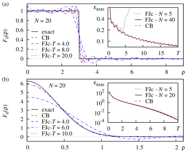
Figure 1: (Color online) Discrete Fourier-Bessel transform (dFBT) for two benchmark transform pairs and different transform parameters $T$ and $N$, following the method of Fisk-Johnson for a continuous objective function discussed in section 3. (a) Transform of the jinc-function discussed in the text. The main plot shows a sequence of extrapolated function values of the transform for differenct choices ot the truncation parameter $T$ at $N=20$ (blue dash-dotted curves; labeled FJc). The result obtained by a straight forward numerical integration of the integral transform is shown as red dashed curve (labeled CB). The inset illustrates the root-mean squared error $\epsilon_{\rm RMS}(T)$ for two choices of $N$. (b) Transform of the Gaussian function discussed in the text. The main plot shows the extrapolated function values for different choices of $T$ at $N=20$ and the inset illustrates $\epsilon_{\rm RMS}$ for two values of $N$.

dFBT of a jinc function -

First we considered the Fourier-Bessel pair

$$f(r)=a_{0}^{2}\,{\rm jinc}(a_{0}r)\quad\Longleftrightarrow\quad F_{0}(\rho)=\theta(\rho-a_{0}),$$ (9)

for $a_{0}=3$, wherein ${\rm jinc}(x)=J_{1}(x)/x$ and $\theta(\cdot)$ signifies the Heavyside step function. While here, the Fisk-Johnson algorithm exploits the possibility to compute $f(r)$ at precisely those sample points required by Eq. (3), the Cree-Bones algorithm used an equispaced grid $\{r_{i}\}_{i=0}^{M-1}$ with, $r_{i}=r_{0}+i\Delta$ and $\Delta=(r_{M-1}-r_{0})/(M-1)$ where $r_{0}=0.01$, $r_{M-1}=20$, $M=1000$. As usual in Fourier-type function approximation, due to the discontinuous nature of $\theta$, we expect this kind of benchmark transform pair to represent a difficult test for any kind of dFBT. Bearing this in mind, the considered transform pair might be regarded as a worst-case use case that might arise in computational biophotonics since a commonly employed irradiation source profile (ISP), referred to as “top-hat” ISP, exhibits the shape of $\theta$ [9, 10]. Consequently, any convolution using such an ISP involves a revese dFBT of the above form.

In Fig. 1(a) we show the result of applying the dFBT to the above jinc-function. In the main plot of Fig. 1(a) we explore the effect a finite truncation threshold $T$ has on the transformed function for the summation threshold $N=20$. Note that for small values of $T$ the Fisk-Johnson dFBT deviates significantly from the exact transform (solid black line). This is due to the assumption that above $T$ the objective function vanishes and, hence, structural details of the jinc-function bejond that threshold are ignored in the transformation process. As the value of $T$ grows larger, the dFBT approximation at sufficiently large $N$ gets increasingly better as shown by the overall decrease of the RMS error in the inset. While, at given $T$, a too small value of $N$ leads to a huge RMS error, reflecting that the truncated Fourier-Bessel series has not converged as in the case of $N=5$, the accuracy of the Fisk-Johnson transform at $N=40$ is similar to that of the (computationally more expensive) Cree-Bones transform. To support intuition, further computer experiments indicate that, e.g., at $T=10$ there exists a narrow threshold range $N=6-12$ within which the RMS error decreases by one order of magnitude (not shown; see discussion below), and where $\epsilon_{\rm RMS}(N>12)\approx 0.12$ (cf. inset of Fig. 1(a)). For completeness, note that for $T=20$ and $N=20$, the Fisk-Johnson and Cree-Bones dFBT agree well as illustrated in the main plot of Fig. 1(a). Both feature Gibbs ringing artifacts that might be expected for this kind of transform pair.

dFBT of a Gaussian function -

Next, we consider the dFBT transform of a Gaussian function

$$f(r)=\exp\{-r^{2}/(4\pi)\}\quad\Longleftrightarrow\quad F_{0}(\rho)=2\pi\exp\{-\pi r^{2}\}.$$ (10)

For the numerical experiments using the Cree-Bones algorithm we again used an equispaced grid $\{r_{i}\}_{i=0}^{M-1}$ with, $r_{i}=r_{0}+i\Delta$ and $\Delta=(r_{M-1}-r_{0})/(M-1)$ where $r_{0}=0.01$, $r_{M-1}=10$, $M=1000$. For this kind of smooth benchmark transform pair we expect the accuracy of the tranform to be even better than in the previous case. This type of objective function might be regarded as a best-case use case that might arise in computational biophotonics since another commonly employed ISP has the shape of a simple Gaussian function [9, 10].

As evident from Fig. 1(b), similar to the previous example, if the truncation threshold $T$ is chosen too small, the transfrom deviates from the exact result since vital parts of the objective function beyond $T$ are ignored. To support intuition, note that $f(r)$ drops to its $1/e$-height at $T=2\pi^{1/2}\approx 3.5$, explaining the deviation of the $T=4$ dFBT approximation to the exact result. However, a visual inspection of the approximation at $T=10$, where one finds $f(0)/f(10)\approx 2.8\cdot 10^{3}$, indicates that it fits the asymptotic result quite well. This “chi-by-eye” result is supported by the relative RMS error illustrated in the inset. Even at small values of the summation trunction parameter $N$, the accuracy of the Fisk-Johnson dFBT improves noticably as $T\to 10$ and approaches the approximation error of the CB transform at a given value of $T$ rapidly as $N$ is adjusted to higher values.

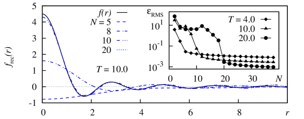
Figure 2: (Color online) Reconstruction $f_{\rm rec}$ of the initial function under a reverse dFBT. The main plot shows the original objective function (solid black curve) and the reconstructed functions at $T=10.0$ for different values of $N$. The inset illustrates the relative RMS error (see Eq. 8) for three choices of the truncation threshold $T$ for $N=2$ through $40$.

Reconstruction of the objective function -

Next, we assess the accuracy of a reconstruction of the objective function under a reverse dFBT implemented according to Eq. (5). Therefore, we first compute the dFBT approximation to the jinc-objective function using the sequence of grid samples required by Eq. (3), where we considered the truncation threshold $T=10.0$ and different values of $N$. The results of a subsequent reverse transformation, computed for a sufficiently sampling density of $x$ via the Fisk-Johnson procedure are summarized in Fig. 2. As evident from the main plot of the figure, the reconstruction of the objective function seems to be quite accurate once the summation truncation parameter exceeds $N=20$. This finding can be put on a more quantitative basis by means of the relative RMS error, reported in the inset of Fig. 2. We find that at $T=10.0$ there exists a narrow threshold range $N=6-12$ within which the RMS error decreases by almost three orders of magnitude from $\epsilon_{\rm RMS}(N=6)\approx 7.7$ to $\epsilon_{\rm RMS}(N=12)\approx 0.007$. For higher (smaller) values of $T$, this threshold range can be seen to shift towards higher (smaller) values of $N$. This is intuitive since at larger values of $T$ more sample points of the transformed domain are necessary to capture the structural details of the underlying function appropriately, thus affecting the convergence of the truncated sums used to approximate the Fourier-Bessel integral transform.

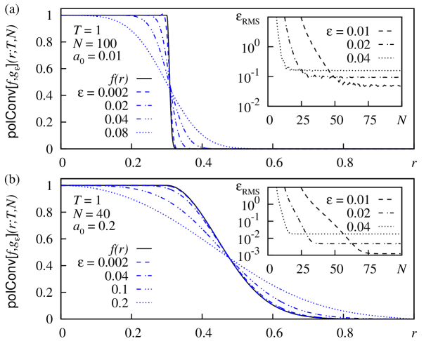
Figure 3: (Color online) Exemplary $2$D polar convolution using the Fisk-Johnson procedure detailed in section 2. The figure illustrates the convolution $h(r)={\mathsf{polConf}}[f,g](r;T,N)$ of a flat-top profile $f(r)$ with a Gaussian approximation $g_{\epsilon}(r)$ to the delta-distribution, see section 3. In the limit $\epsilon\to 0$ we expect to find $h(r)\to f(r)$. (a) Convolution using the “steep” flat-top parameters $r_{0}=0.3$, $a_{0}=0.01$ and truncation thresholds $T=1$, $N=100$ for different values of $\epsilon$. The inset shows the relative RMS errors for the approximation of $f(r)$ by $h(r)$ as function of the summation truncation parameter $N$. (b) same as (a) for “smooth” flat top parameters $r_{0}=0.3$, $a_{0}=0.2$ and summation truncation parameter $N=40$.

Exemplary polar convolution -

Finally, we test the performance of the dFBT for the purpose of $2$D polar convolution. Therefore, we consider the two functions

$$f(r)=\cases{1&for $r\leq r_{0}$\\ \exp\{-(r-r_{0})^{2}/a_{0}^{2}\}&for $r>r_{0}$\\ },$$ (11a)

$$g_{\epsilon}(r)=(2\pi\epsilon^{2})^{-1}\exp\{-r^{2}/(2\epsilon^{2}))\}.$$ (11b)

and follow the procedural description detailed in section 2 to compute ${\mathsf{polConv}}[f,g_{\epsilon}]$. Note that Eq. (11a) represents a “flat-top” ISP, i.e. a top-hat function with a smooth roll-off, consistent with actual beam profiles observed in laboratory experiments, see Refs. [11, 12, 9, 13, 14] that report on flat-top ISPs with parameter ratio in the range $r_{0}/a_{0}=1-10$. Further, Eq. (11b) signifies a Gaussian approximation to a $2$D delta-function, attained in the limit $\epsilon\to 0$. Hence, we expect to find $\lim_{\epsilon\to 0}{\mathsf{polConv}}[f,g_{\epsilon}](r)=f(r)$. In this question, Fig. 3 illustrates the accuracy of the Fisk-Johnson convolution procedure for a “steep” example with $r_{0}/a_{0}=300$ and a “smooth” example with $r_{0}/a_{0}=1.5$, see Figs. 3(a) and (b), respectively. As evident from the scaling behavior of the associated RMS error between $f(r)$ and $h(r)$ (shown in the inset of the subfigures), the accuracy of the approximation at fixed $T=1.0$ and given $\epsilon$ increases as the summation truncation parameter $N$ increases, saturating at a characteristic limiting value $N_{\epsilon}$. As $\epsilon$ decreases, i.e. the closer $g_{\epsilon}(r)$ approximates a delta-function, the approximation error of $h(r)$ also decreases. Bearing in mind the above results for the forward and reverse dFBT it does not come as a surprise that the polar convolution of a “smooth” objective function with a delta-function is more accurate than that of a “steep” objective function.

4 Application to beam-shape convolution in polar coordinates

An application of the efficient Fisk-Johnson polar convolution algorithm to a particular problem in computational biophotonics is illustrated in the remainder. It provides a solution to the issue of computing the material response to custom radially symmetric laser beams of finite extend for layered homogeneous media, given the corresponding Green’s function response of the medium. To illustrate the computational procedure we considered the simple but paradigmatic case of a semi-infinite medium with a refractive-index-mismatched boundary. For the optical parameters we used the relative refractive indices $n=1.0$ (for the ambient medium) and $n=1.37$ as well as the absorption coefficient $\mu_{\rm a}=0.1\,{\rm cm^{-1}}$, scattering coefficient $\mu_{\rm s}=10.0\,{\rm cm^{-1}}$ and values of the anisotropy parameter $g\in[0.1,0.95]$.

Table 1: Characteristic lengthscales [15] for light transport in the considered tissue setup and homogeneous grid parameter for discretization of the source volume using MCML [6]. From left to right: anisotropy parameter $g$, mean free path (mfp) length $\ell_{\rm mfp}$, transport mfp $\tilde{\ell}_{\rm mfp}$, penetration depth $d_{\rm p}$ and grid parameters for the cylindrical sampling lattice.

				$z$-axis			$r$-axis
$g$	$\ell_{\rm mfp}$	$\tilde{\ell}_{\rm mfp}$	$d_{\rm p}$	$N_{z}$	$\Delta_{z}$	$z_{\rm max}$	$N_{r}$	$\Delta_{r}$	$r_{\rm max}$
	(cm)	(cm)	(cm)	(bins)	(cm)	(cm)	(bins)	(cm)	(cm)
0.10	0.099	0.110	0.605	363	0.005	1.815	1000	0.002	2.0
0.70	0.099	0.323	1.037	622	0.005	3.11	1000	0.0033	3.3
0.90	0.099	0.909	1.741	1044	0.005	5.22	1000	0.0053	5.4
0.95	0.099	1.667	2.357	1414	0.005	7.07	1000	0.0073	7.3

Monte Carlo modelling of the Greens function response -

For our numerical experiments we computed the Green’s function $G$ of the absorbed energy density for the above setup as the material response to an infinitely thin “pencil” beam using the publicly available C code MCML [6]. It solves the problem of steady-state light transport in terms of a Monte Carlo approach to photon migration in layered media and provides the accumulated observables on a homogeneous polar grid, i.e. $G\equiv G(r,z)$. For our numerical experiments we used the simulation parameters listed in Tab. 1. In setting up the discretized source volume we made sure the maximal $z$-depth $z_{\rm max}$ and $r$-range $r_{\rm max}$ exceed the penetration depth $d_{\rm p}$ of photons within the medium by a factor of three at least. Note that for extended beam profiles and not too close to the material surface, $d_{\rm p}$ refers to the intrinsic length-scale after which the fluence-rate along the beam-axis reduces to its $1/e$-value [6, 15]. For completeness, one might perform the numerical experiments as well by one of MCMLs descendants designed for layered homogeneous media, as, e.g., GPU-MCML [16].

Material response to laser beams with finite extend -

In order to obtain the desired material response $W(r,z)$ to an extended radially symmetric laser beam, the Green’s function $G(r,z)$ needs to be convolved using an appropriate transverse ISP $f(r)$. In principle this can be done using the publicly available C code CONV [10], that implements a top-hat and a Gaussian ISP. However, note that since CONV features only these two ISPs it is of rather limited use. Albeit allowing for a highly efficient direct convolution involving the solution of $1$D integrals only, both beam profiles are not consistent with actual profiles observed in laboratory experiments, see Refs. [11, 12, 9, 13, 14]. Further, on a more general basis, a computationally efficient and more versatile solution procedure that allows for convolution with custom ISPs seems to be of value.

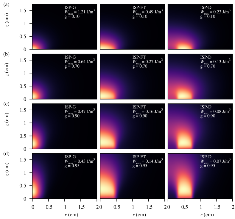
Figure 4: (Color online) Illustration of the beam shape convolution procedure for a Gaussian ISP (G; a special case of Eq. (11m) with $r_{0}=0$ and $r_{1}=0$) with parameter $a_{1}=0.25$, flat-Top ISP (FT; a special case of Eq. (11m) with $r_{0}=0$) with parameters $r_{1}=0.4$ and $a_{1}=0.1$, and donut (D) ISP with parameters $r_{0}=0.25$, $r_{1}=0.6$ and $a_{0}=a_{1}=0.05$ considering four different values of the anisotropy parameter $g$. (a) from left to right (ltr): G, FT and D ISP for $g=0.10$, (b) ltr: G, FT and D ISP for $g=0.70$, (c) ltr: G, FT and D ISP for $g=0.90$, (d) ltr: G, FT and D ISP for $g=0.95$. The maximal value of absorbed laser energy $W_{\rm max}~{}({\rm J/m^{3}})$ for each configuration, indicated by the brightest color, is listed within the individual subfigures.

In this regard we follow a different approach by solving the 2D convolution problem in terms of the Fourier-Bessel transform in polar coordinates [10, 5]

$$W(r,z)=\mathsf{polConv}[f,G](r,z)=2\pi f_{0}\int_{0}^{\infty}G_{0}(\rho,z)F_{0}(\rho)J_{0}(\rho r)\rho~{}{\rm d}\rho,$$ (11l)

following the Fisk-Johnson discretization procedure detailed in section 2. Therein, $f(r)$ signifies a custom “donut” ISP

$$f(r)=\cases{\exp\{-(r-r_{0})^{2}/a_{0}^{2}\}&for $r<r_{0}$\\ 1&for $r_{0}\leq r\leq r_{1}$\\ \exp\{-(r-r_{1})^{2}/a_{1}^{2}\}&for $r>r_{1}$\\ },$$ (11m)

and $G$ stands for the laser absorption Green’s function computed for an infinitely narrow laser beam, incident upon the material surface. The respective dFBTs are given by $F_{0}$ and $G_{0}$. In the above equation, $f_{0}$ allows to scale the beam intensity to achieve a total beam power $P$ via

$$f_{0}=P~{}\big{[}2\pi\int_{0}^{\infty}\,r~{}f(r)~{}{\rm d}r\big{]}^{-1}.$$ (11n)

Note that this yields a general purpose routine that allows for quite arbitrary beam profiles, only required to obey the integrability conditions of a Fourier-Bessel transform. As a technicality, note that the dFBT $F_{0}$ of the continuous ISP $f$, computed using the $O(M^{2})$ algorithm Eq. (3), can be reused at each value of $z$. In contrast to the later function, since $G(r,z)$ is known at a finite number of sample points only, its dFBT $G_{0}$ is obtained via the $O(NM)$ algorithm Eq. (4).

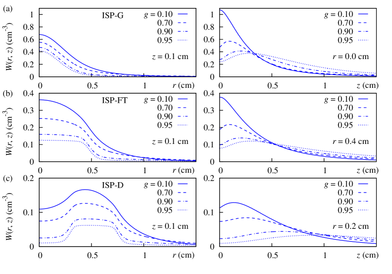
Figure 5: (Color online) Absorbed energy density $W(r,z)$ at fixed $z$- and $r$-slices for the three ISPs used in section 4. (a) Gaussian ISP at $z=0.1\,{\rm{cm}}$ (left) and $r=0.0\,{\rm{cm}}$ (right) considering different values of the anisotropy $g$, (b) Flat-top ISP at $z=0.1\,{\rm{cm}}$ (left) and $r=0.4\,{\rm{cm}}$ (right), (c) Donut ISP at $z=0.1\,{\rm{cm}}$ (left) and $r=0.2\,{\rm{cm}}$ (right).

In Fig. 4 we illustrate the Fisk-Johnson convolution procedure for various anisotropy parameters and three beam shapes: (i) a Gaussian ISP (G), i.e. a special case of Eq. (11m) with $r_{0}=0$, $r_{1}=0$ and $a_{1}=0.25$ where we used the dFBT parameters $T=4.0$ and $N=40$, (ii) a flat-Top ISP (FT), a special case of Eq. (11m) with $r_{0}=0$, $r_{1}=0.4$ and $a_{1}=0.1$ using $T=4.0$ and $N=80$, and, (iii) a donut (D) ISP with parameters $r_{0}=0.25$, $r_{1}=0.6$ and $a_{0}=a_{1}=0.05$ using $T=4.0$ and $N=150$. Based on the parameter studies for the forward and reverse dFBT reported in section 3, and by monitoring the rms error for the forward and immediate backtransformation of the beam profile, yielding $\epsilon_{\rm rms}<10^{-6}$ (ISP-G), $\epsilon_{\rm rms}=0.003$ (ISP-FT), and, $\epsilon_{\rm rms}=0.008$ (ISP-D), we opted for the truncation threshold $T$ and summation truncation parameters $N$ listed above. To clarify the behavior of $W(r,z)$ and to illustrate the decrease of $W_{\rm max}$ as function of $g$, samples of the absorbed energy density at fixed $z$- and $r$-slices are shown in Fig. 5. As one might intuitively expect, Figs. 4 and 5 reveal two tendencies: (i) for increasing anisotropy $g$, the smoothing of $W(r,z)$ due to scattering reduces and its absolute values decreases since backscattering is suppressed, and, (ii) for increasing $g$, the maximum $W_{\rm max}$ shifts towards deeper values of $z$ since scattering is focused on the forward direction. A thorough discussion of the characteristics of extended beam profiles and their use in tissue optics and optoacoustic signal prediction for multilayered tissues will be presented elsewhere [17].

5 Summary and conclusions

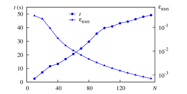
Figure 6: (Color online) Accuracy and computational efficiency of the Fisk-Johnson polar convolution as function of the summation truncation parameter $N$ at fixed $T=4.0$ for the flat-top ISP. The reconstruction RMS error of the ISP decreases below $10^{-2}$ at approximately $N=50$. At this point, the convolution procedure terminates after $t(50)\approx 17\,{\rm{s}}$. For comparison: the Cree-Bones procedure used for benchmarking terminates after time $t_{\rm{CB}}\approx 326\,{\rm{s}}$, highlighting the performance of the Fisk-Johnson algorithm.

In the presented article we discussed the Fisk-Johnson procedure for computing a $2$D polar convolution of two radially symmetric functions, based on efficient discrete approximations to the forward and reverse Fourier-Bessel integral transform. We assessed the efficiency and accuracy of the forward transform, reverse transform and polar convolution on a set of test functions and applied the method to a problem from computational biophotonics. Therein, the aim was to convolve the Green’s function material response to an infinitely thin laser beam to an extended beam profile. From a point of view of computational efficiency, the presented procedure resides between the highly efficient but ISP-restricted direct convolution (implemented in terms of the CONV code [10]) and the inefficient but accurate straight forward numerical quadrature used for benchmarking in section 3. Bear in mind that (time) efficiency is an issue: so as to complete the convolution procedure for, say, the sampled source volume at $g=0.95$, an individual convolution has to be carried out for a sequence of $N_{z}=1414$ consecutive values of $z$, each involving a number of $N_{r}=1000$ sample points $r$, see Tab. 1. For the exemplary case of the previous flat-top beam profile, Fig. 6 reveals that the completion time of the Fisk-Johnson convolution procedure is linear in $M$ with $t(N)\approx 0.34(1)N\,{\rm{s}}$. In particular, the reconstruction error of the ISP decreases below $10^{-2}$ at approximately $N=50$. At this value of $N$, the Fisk-Johnson procedure terminates after $\approx 17\,{\rm{s}}$. In contrast, note that the Cree-Bones procedure used for benchmarking in section 3 terminates after $\approx 326\,{\rm{s}}$, highlighting the efficiency of the Fisk-Johnson polar convolution for the considered application.

Albeit the scientific literature frequently features new algorithms to compute the above (and further related) transforms for particular scientific applications, their thorough exploration and implementation in terms of, say, symbolic computer algebra is rather recent [18]. Since the discrete Fourier-Bessel transform and the polar convolution are valuable computational tools for the solution of many physical problems with axial symmetry, and so as to follow the ideal of guaranteeing reproducible results in scientific publications [19, 20], we considered it useful to make the research-code for the presented study, along with all scripts needed to reproduce all figures, publicly available on one of the authors gitHub profile [21].

References

References

- [1] James D Talman. Numerical fourier and bessel transforms in logarithmic variables. Journal of Computational Physics, 29:35, 1978.
- [2] H. Fisk Johnson. An improved method for computing a discrete Hankel transform. Computer Physics Communications, 43:181, 1987.
- [3] M. Guizar-Sicairos and J. C. Gutiérrez-Vega. Computation of quasi-discrete hankel transforms of integer order for propagating optical wave fields. J. Opt. Soc. Am. A, 21(1):53, 2004.
- [4] N. Baddour and U. Chouinard. Theory and operational rules for the discrete Hankel transform. J. Opt. Soc. Am. A, 32:611, 2015.
- [5] N. Baddour. Operational and convolution properties of two-dimensional Fourier transforms in polar coordinates. J. Opt. Soc. Am. A, 26:1767, 2009.
- [6] L. Wang, S. L. Jacques, and L. Q. Zheng. MCML - Monte Carlo modeling of photon transport in multi-layered tissues. Computer Methods and Programs in Biomedicine, 47:131, 1995.
- [7] Note that in Ref. [5], Eq. 6 is formulated in terms of the D Fourier transform of , which, in case of a radially symmetric functions is related to the Fourier-Bessel transform via .
- [8] M. J. Cree and P. J. Bones. Algorithms to numerically evaluate the Hankel transform. Computers Math. Applic., 26(1):1, 1993.
- [9] G. Paltauf and H. Schmidt-Kloiber. Pulsed optoacoustic characterization of layered media. Journal of Applied Physics, 88:1624–1631, 2000.
- [10] L. Wang, S. L. Jacques, and L. Q. Zheng. CONV - convolution for responses to a finite diameter photon beam incident on multi-layered tissues. Computer Methods and Programs in Biomedicine, 54:141, 1997. For source code, see: http://omlc.org/software/mc/.
- [11] G. Paltauf and H. Schmidt-Kloiber. Measurement of laser-induced acoustic waves with a calibrated optical transducer. Journal of Applied Physics, 82:1525, 1997.
- [12] G. Paltauf, H. Schmidt-Kloiber, and M. Frenz. Photoacoustic waves excited in liquids by fiber-transmitted laser pulses. J. Acoust. Soc. Am., 104:890–897, 1998.
- [13] B. D’Alessandro and A. P. Dhawan. 3-D Volume Reconstruction of Skin Lesions for Melanin and Blood Volume Estimation and Lesion Severity Analysis. IEEE Transactions on Medical Imaging, 31:2083, 2012.
- [14] E. Blumenröther, O. Melchert, M. Wollweber, and B. Roth. Detection, numerical simulation and approximate inversion of optoacoustic signals generated in multi-layered PVA hydrogel based tissue phantoms. Photoacoustics, 4:125–132, 2016.
- [15] B. C. Wilson and S. L. Jacques. Optical reflectance and transmittance of tissues: principles and applications. IEEE Journal of Quantum Electronics, 26:2186, 1990.
- [16] E. Alerstam, W. C. Y. Lo, T. D. Han, J. Rose, S. Andersson-Engels, and L. Lilge. Next-generation acceleration and code optimization for light transport in turbid media using gpus. Biomed. Opt. Express, 1:658–675, 2010.
- [17] O. Melchert, M. Wollweber, and B. Roth. (in preparation).
- [18] E. Dovlo and N. Baddour. Toolbox for the Computation of 2D Fourier Transforms in Polar Coordinates via Maple. Journal of Open Research Software, 3:e3, 2015.
- [19] G. K. Sandve, A. Nekrutenko, J. Taylor, E. Hovig, and P. E. Bourne. Ten simple rules for reproducible computational research. PLoS Computational Biology, 9:e1003285, 2013.
- [20] N. Barnes. Publish your computer code: it is good enough. Nature, 467:753, 2010.
- [21] A Python implementation of our research code that might be used to reproduce this paper’s results can be found at at https://github.com/omelchert/dFBT-FJ.git.