An epidemic model for cholera
with optimal control treatment

Abstract

We propose a mathematical model for cholera with treatment through quarantine. The model is shown to be both epidemiologically and mathematically well posed. In particular, we prove that all solutions of the model are positive and bounded; and that every solution with initial conditions in a certain meaningful set remains in that set for all time. The existence of unique disease-free and endemic equilibrium points is proved and the basic reproduction number is computed. Then, we study the local asymptotic stability of these equilibrium points. An optimal control problem is proposed and analyzed, whose goal is to obtain a successful treatment through quarantine. We provide the optimal quarantine strategy for the minimization of the number of infectious individuals and bacteria concentration, as well as the costs associated with the quarantine. Finally, a numerical simulation of the cholera outbreak in the Department of Artibonite (Haiti), in 2010, is carried out, illustrating the usefulness of the model and its analysis.

Keywords: SIQRB cholera model, basic reproduction number, disease-free and endemic equilibria, local asymptotic stability, optimal control, numerical case study of Haiti.

Mathematics Subject Classification 2010: 34C60, 49K15, 92D30.

1 Introduction

Cholera is an acute diarrhoeal illness caused by infection of the intestine with the bacterium Vibrio cholerae, which lives in an aquatic organism. The ingestion of contaminated water can cause cholera outbreaks, as John Snow proved, in 1854 [27]. This is a way of transmission of the disease, but others exist. For example, susceptible individuals can become infected if they contact with infected individuals. If individuals are at an increased risk of infection, then they can transmit the disease to other persons that live with them by reflecting food preparation or using water storage containers [27]. An individual can be infected with or without symptoms. Some symptoms are watery diarrhoea, vomiting and leg cramps. If an infected individual does not have treatment, then he becomes dehydrated, suffering of acidosis and circulatory collapse. This situation can lead to death within 12 to 24 hours [21, 27]. Some studies and experiments suggest that a recovered individual can be immune to the disease during a period of 3 to 10 years. Recent researches suggest that immunity can be lost after a period of weeks to months [22, 27].

Since 1979, several mathematical models for the transmission of cholera have been proposed: see, e.g., [1, 2, 7, 10, 12, 15, 20, 21, 22, 24, 27] and references cited therein. In [22], the authors propose a SIR (Susceptible–Infectious–Recovered) type model and consider two classes of bacterial concentrations (hyperinfectious and less-infectious) and two classes of infectious individuals (asymptomatic and symptomatic). In [27], another SIR-type model is proposed that incorporates, using distributed delays, hyperinfectivity (where infectivity varies with the time since the pathogen was shed) and temporary immunity. The authors of [21] incorporate in a SIR-type model public health educational campaigns, vaccination, quarantine and treatment, as control strategies in order to curtail the disease.

The use of quarantine for controlling epidemic diseases has always been controversial, because such strategy raises political, ethical and socioeconomic issues and requires a careful balance between public interest and individual rights [30]. Quarantine was adopted as a mean of separating persons, animals and goods that may have been exposed to a contagious disease. Since the fourteenth century, quarantine has been the cornerstone of a coordinated disease-control strategy, including isolation, sanitary cordons, bills of health issued to ships, fumigation, disinfection and regulation of groups of persons who were believed to be responsible for spreading of the infection [19, 30]. The World Health Organization (WHO) does not recommend quarantine measures and embargoes on the movement of people and goods for cholera. However, cholera is still on the list of quarantinable diseases of the EUA National Archives and Records Administration [5]. In this paper, we propose a SIQR (Susceptible–Infectious–Quarantined–Recovered) type model, where it is assumed that infectious individuals are subject to quarantine during the treatment period.

Optimal control is a branch of mathematics developed to find optimal ways to control a dynamic system [6, 9, 25]. There are few papers that apply optimal control to cholera models [22]. Here we propose and analyze one such optimal control problem, where the control function represents the fraction of infected individuals $I$ that will be submitted to treatment in quarantine until complete recovery. The objective is to find the optimal treatment strategy through quarantine that minimizes the number of infected individuals and the bacterial concentration, as well as the cost of interventions associated with quarantine.

Between 2007 and 2011, several cholera outbreaks occurred, namely in Angola, Haiti and Zimbabwe [27]. In Haiti, the first cases of cholera happened in Artibonite Department on 14th October 2010. The disease propagated along the Artibonite river and reached several departments. Only within one month, all departments had reported cases in rural areas and places without good conditions of public health [33]. In this paper, we provide numerical simulations for the cholera outbreak in the Department of Artibonite, from $1$st November 2010 until $1$st May 2011 [33]. Our work is of great significance, because it provides an approach to cholera with big positive impact on the number of infected individuals and on the bacterial concentration. This is well illustrated with the real data of the cholera outbreak in Haiti that occurred in 2010. More precisely, we show that the number of infectious individuals decreases significantly and that the bacterial concentration is a strictly decreasing function, when our control strategy is applied.

The paper is organized as follows. In Section 2, we formulate our model for cholera transmission dynamics. We analyze the positivity and boundedness of the solutions, as well as the existence and local stability of the disease-free and endemic equilibria, and we compute the basic reproduction number in Section 3. In Section 4, we propose and analyze an optimal control problem. Section 5 is devoted to numerical simulations. We end with Section 6, by deriving some conclusions about the inclusion of quarantine in treatment.

2 Model formulation

We propose a SIQR (Susceptible–Infectious–Quarantined–Recovered) type model and consider a class of bacterial concentration for the dynamics of cholera. The total population $N(t)$ is divided into four classes: susceptible $S(t)$, infectious with symptoms $I(t)$, in treatment through quarantine $Q(t)$ and recovered $R(t)$ at time $t$, for $t\geq 0$. Furthermore, we consider a class $B(t)$ that reflects the bacterial concentration at time $t$. We assume that there is a positive recruitment rate $\Lambda$ into the susceptible class $S(t)$ and a positive natural death rate $\mu$, for all time $t$ under study. Susceptible individuals can become infected with cholera at rate $\frac{\beta B(t)}{\kappa+B(t)}$ that is dependent on time $t$. Note that $\beta>0$ is the ingestion rate of the bacteria through contaminated sources, $\kappa$ is the half saturation constant of the bacteria population and $\frac{B(t)}{\kappa+B(t)}$ is the possibility of an infected individual to have the disease with symptoms, given a contact with contaminated sources [21]. Any recovered individual can lose the immunity at rate $\omega$ and therefore becomes susceptible again. The infected individuals can accept to be in quarantine during a period of time. During this time they are isolated and subject to a proper medication, at rate $\delta$. The quarantined individuals can recover at rate $\varepsilon$. The disease-related death rates associated with the individuals that are infected and in quarantine are $\alpha_{1}$ and $\alpha_{2}$, respectively. Each infected individual contributes to the increase of the bacterial concentration at rate $\eta$. On the other hand, the bacterial concentration can decrease at mortality rate $d$. These assumptions are translated in the following mathematical model:

$$\begin{cases}S^{\prime}(t)=\Lambda-\displaystyle\frac{\beta B(t)}{\kappa+B(t)}S(t)+\omega R(t)-\mu S(t),\\ I^{\prime}(t)=\displaystyle\frac{\beta B(t)}{\kappa+B(t)}S(t)-(\delta+\alpha_{1}+\mu)I(t),\\ Q^{\prime}(t)=\delta I(t)-(\varepsilon+\alpha_{2}+\mu)Q(t),\\ R^{\prime}(t)=\varepsilon Q(t)-(\omega+\mu)R(t),\\ B^{\prime}(t)=\eta I(t)-dB(t).\end{cases}$$ (1)

3 Model analysis

Throughout the paper, we assume that the initial conditions of system (1) are nonnegative:

$$S(0)=S_{0}\geq 0\,,\quad I(0)=I_{0}\geq 0\,,\quad Q(0)=Q_{0}\geq 0\,,\quad R(0)=R_{0}\geq 0\,,\quad B(0)=B_{0}\geq 0\,.$$ (2)

3.1 Positivity and boundedness of solutions

Our first lemma shows that the considered model (1)–(2) is biologically meaningful.

Lemma 1.

The solutions $(S(t),I(t),Q(t),R(t),B(t))$ of system (1) are nonnegative for all $t\geq 0$ with nonnegative initial conditions (2) in $(\mathbb{R}_{0}^{+})^{5}$.

Proof.

We have

$$\begin{cases}\frac{dS(t)}{dt}\Bigg{|}_{\xi(S)}&=\Lambda+\omega R(t)>0\,,\\ \frac{dI(t)}{dt}\Bigg{|}_{\xi(I)}&=\frac{\beta B(t)}{\kappa+B(t)}S(t)>0\,,\\ \frac{dQ(t)}{dt}\Bigg{|}_{\xi(Q)}&=\delta I(t)>0\,,\\ \frac{dR(t)}{dt}\Bigg{|}_{\xi(R)}&=\varepsilon Q(t)>0\,,\\ \frac{dB(t)}{dt}\Bigg{|}_{\xi(B)}&=\eta I(t)>0\,,\end{cases}$$

where $\xi(\upsilon)=\left\{\upsilon(t)=0\text{ and }S,I,Q,R,B\in C(\mathbb{R}_{0}^{+},\mathbb{R}_{0}^{+})\right\}$ and $\upsilon\in\{S,I,Q,R,B\}$. Therefore, due to Lemma 2 in [34], any solution of system (1) is such that $(S(t),I(t),Q(t),R(t),B(t))\in(\mathbb{R}_{0}^{+})^{5}$ for all $t\geq 0$. ∎

Next Lemma 2 shows that it is sufficient to consider the dynamics of the flow generated by (1)–(2) in a certain region $\Omega$.

Lemma 2.

Let

$$\Omega_{H}=\left\{(S,I,Q,R)\in\left(\mathbb{R}_{0}^{+}\right)^{4}\,|\,0\leq S(t)+I(t)+Q(t)+R(t)\leq\frac{\Lambda}{\mu}\right\}$$ (3)

and

$$\Omega_{B}=\left\{B\in\mathbb{R}_{0}^{+}\,|\,0\leq B(t)\leq\frac{\Lambda\eta}{\mu d}\right\}.$$ (4)

Define

$$\Omega=\Omega_{H}\times\Omega_{B}.$$ (5)

If $N(0)\leq\frac{\Lambda}{\mu}$ and $B(0)\leq\frac{\Lambda\eta}{\mu d}$, then the region $\Omega$ is positively invariant for model (1) with nonnegative initial conditions (2) in $(\mathbb{R}_{0}^{+})^{5}$.

Proof.

Let us split system (1) into two parts: the human population, i.e., $S(t)$, $I(t)$, $Q(t)$ and $R(t)$, and the pathogen population, i.e., $B(t)$. Adding the first four equations of system (1) gives

$$N^{\prime}(t)=S^{\prime}(t)+I^{\prime}(t)+Q^{\prime}(t)+R^{\prime}(t)=\Lambda-\mu N(t)-\alpha_{1}I(t)-\alpha_{2}Q(t)\leq\Lambda-\mu N(t)\,.$$

Assuming that $N(0)\leq\frac{\Lambda}{\mu}$, we conclude that $N(t)\leq\frac{\Lambda}{\mu}$. For this reason, (3) defines the biologically feasible region for the human population. For the pathogen population, it follows that

$$B^{\prime}(t)=\eta I(t)-dB(t)\leq\eta\frac{\Lambda}{\mu}-dB(t)\,.$$

If $B(0)\leq\frac{\Lambda\eta}{\mu d}$, then $B(t)\leq\frac{\Lambda\eta}{\mu d}$ and, in agreement, (4) defines the biologically feasible region for the pathogen population. From (3) and (4), we know that $N(t)$ and $B(t)$ are bounded for all $t\geq 0$. Therefore, every solution of system (1) with initial condition in $\Omega$ remains in $\Omega$. ∎

In region $\Omega$ defined by (5), our model is epidemiologically and mathematically well posed in the sense of [11]. In other words, every solution of the model (1) with initial conditions in $\Omega$ remains in $\Omega$ for all $t\geq 0$.

3.2 Equilibrium points and stability analysis

The disease-free equilibrium (DFE) of model (1) is given by

$$E^{0}=(S^{0},I^{0},Q^{0},R^{0},B^{0})=\left(\frac{\Lambda}{\mu},0,0,0,0\right).$$ (6)

Next, following the approach of [21, 32], we compute the basic reproduction number $R_{0}$.

Proposition 3 (Basic reproduction number of (1)).

The basic reproduction number of model (1) is given by

$$R_{0}=\frac{\beta\Lambda\eta}{\mu\kappa d(\delta+\alpha_{1}+\mu)}.$$ (7)

Proof.

Consider that $\mathscr{F}_{i}(t)$ is the rate of appearance of new infections in the compartment associated with index $i$, $\mathscr{V}_{i}^{+}(t)$ is the rate of transfer of “individuals” into the compartment associated with index $i$ by all other means and $\mathscr{V}_{i}^{-}(t)$ is the rate of transfer of “individuals” out of compartment associated with index $i$. In this way, the matrices $\mathscr{F}(t)$, $\mathscr{V}^{+}(t)$ and $\mathscr{V}^{-}(t)$, associated with model (1), are given by

$$\mathscr{F}(t)=\left[\begin{matrix}0\\ \displaystyle\frac{\beta B(t)S(t)}{\kappa+B(t)}\\ 0\\ 0\\ 0\end{matrix}\right],\quad\mathscr{V}^{+}(t)=\left[\begin{matrix}\Lambda+\omega R(t)\\ 0\\ \delta I(t)\\ \varepsilon Q(t)\\ \eta I(t)\end{matrix}\right]\quad\text{ and }\quad\mathscr{V}^{-}(t)=\left[\begin{matrix}\displaystyle\frac{\beta B(t)S(t)}{\kappa+B(t)}+\mu S(t)\\ a_{1}I(t)\\ a_{2}Q(t)\\ a_{3}R(t)\\ dB(t)\end{matrix}\right],$$

where

$$a_{1}=\delta+\alpha_{1}+\mu,\quad a_{2}=\varepsilon+\alpha_{2}+\mu\ \text{ and }\ a_{3}=\omega+\mu.$$ (8)

Therefore, considering $\mathscr{V}(t)=\mathscr{V}^{-}(t)-\mathscr{V}^{+}(t)$, we have that

$$\left[\begin{matrix}S^{\prime}(t)&I^{\prime}(t)&Q^{\prime}(t)&R^{\prime}(t)&B^{\prime}(t)\end{matrix}\right]^{T}=\mathscr{F}(t)-\mathscr{V}(t).$$

The Jacobian matrices of $\mathscr{F}(t)$ and of $\mathscr{V}(t)$ are, respectively, given by

$$F=\left[\begin{matrix}0&0&0&0&0\\ \displaystyle\frac{\beta B(t)}{\kappa+B(t)}&0&0&0&\displaystyle\frac{\beta\kappa S(t)}{(\kappa+B(t))^{2}}\\ 0&0&0&0&0\\ 0&0&0&0&0\\ 0&0&0&0&0\\ \end{matrix}\right]$$

and

$$V=\left[\begin{matrix}\displaystyle\frac{\beta B(t)}{\kappa+B(t)}+\mu&0&0&-\omega&\displaystyle\frac{\beta\kappa S(t)}{(\kappa+B(t))^{2}}\\ 0&a_{1}&0&0&0\\ 0&-\delta&a_{2}&0&0\\ 0&0&-\varepsilon&a_{3}&0\\ 0&-\eta&0&0&d\\ \end{matrix}\right].$$

In the disease-free equilibrium $E^{0}$ (6), we obtain the matrices $F_{0}$ and $V_{0}$ given by

$$F_{0}=\left[\begin{matrix}0&0&0&0&0\\ 0&0&0&0&\displaystyle\frac{\beta\Lambda}{\mu\kappa}\\ 0&0&0&0&0\\ 0&0&0&0&0\\ 0&0&0&0&0\\ \end{matrix}\right]\quad\text{ and }\quad V_{0}=\left[\begin{matrix}\mu&0&0&-\omega&\displaystyle\frac{\beta\Lambda}{\mu\kappa}\\ 0&a_{1}&0&0&0\\ 0&-\delta&a_{2}&0&0\\ 0&0&-\varepsilon&a_{3}&0\\ 0&-\eta&0&0&d\\ \end{matrix}\right].$$

The basic reproduction number of model (1) is then given by

$$R_{0}=\rho(F_{0}V_{0}^{-1})=\frac{\beta\Lambda\eta}{\mu\kappa da_{1}}=\frac{\beta\Lambda\eta}{\mu\kappa d(\delta+\alpha_{1}+\mu)}.$$

This concludes the proof. ∎

Now we prove the local stability of the disease-free equilibrium $E^{0}$.

Theorem 4 (Stability of the DFE (6)).

The disease-free equilibrium $E^{0}$ of model (1) is

1. Locally asymptotic stable, if $\beta\Lambda\eta<\mu\kappa d(\delta+\alpha_{1}+\mu)$;

2. Unstable, if $\beta\Lambda\eta>\mu\kappa d(\delta+\alpha_{1}+\mu)$.

Moreover, if $\beta\Lambda\eta=\mu\kappa d(\delta+\alpha_{1}+\mu)$, then a critical case occurs.

Proof.

The characteristic polynomial associated with the linearized system of model (1) is given by

$$p(\chi)=\det(F_{0}-V_{0}-\chi I_{5}).$$

In order to compute the roots of polynomial $p$, we have that

$$\left|\begin{matrix}-\mu-\chi&0&0&\omega&-\displaystyle\frac{\beta\Lambda}{\mu\kappa}\\[7.11317pt] 0&-a_{1}-\chi&0&0&\displaystyle\frac{\beta\Lambda}{\mu\kappa}\\[7.11317pt] 0&\delta&-a_{2}-\chi&0&0\\[7.11317pt] 0&0&\varepsilon&-a_{3}-\chi&0\\[7.11317pt] 0&\eta&0&0&-d-\chi\end{matrix}\right|=0,$$

that is,

$$\chi=-\mu\vee\chi=-a_{2}\vee\chi=-a_{3}\vee\tilde{p}(\chi)=\chi^{2}+(a_{1}+d)\chi+a_{1}d-\frac{\beta\Lambda\eta}{\mu\kappa}=0.$$

By Routh’s criterion (see, e.g., p. 55–56 of [23]), if all coefficients of polynomial $\tilde{p}(\chi)$ have the same signal, then the roots of $\tilde{p}(\chi)$ have negative real part and, consequently, the DFE $E^{0}$ is locally asymptotic stable. The coefficients of $\tilde{p}(\chi)$ are $\tilde{p}_{1}=1>0$, $\tilde{p}_{2}=a_{1}+d>0$ and $\tilde{p}_{3}=a_{1}d-\frac{\beta\Lambda\eta}{\mu\kappa}$. Therefore, the DFE $E^{0}$ is

1. Locally asymptotic stable, if $a_{1}d-\frac{\beta\Lambda\eta}{\mu\kappa}>0\Leftrightarrow\beta\Lambda\eta<\mu\kappa d(\delta+\alpha_{1}+\mu)$;

2. Unstable, if $a_{1}d-\frac{\beta\Lambda\eta}{\mu\kappa}<0\Leftrightarrow\beta\Lambda\eta>\mu\kappa d(\delta+\alpha_{1}+\mu)$.

A critical case is obtained if $a_{1}d=\frac{\beta\Lambda\eta}{\mu\kappa}\Leftrightarrow\beta\Lambda\eta=\mu\kappa d(\delta+\alpha_{1}+\mu)$. ∎

Next we prove the existence of an endemic equilibrium when the basic reproduction number (7) is greater than one.

Proposition 5 (Endemic equilibrium).

If $R_{0}>1$, then the model (1) has an endemic equilibrium given by

$$E^{*}=(S^{*},I^{*},Q^{*},R^{*},B^{*})=\left(\frac{\Lambda a_{1}a_{2}a_{3}}{D},\frac{\Lambda a_{2}a_{3}\lambda^{*}}{D},\frac{\Lambda\delta a_{3}\lambda^{*}}{D},\frac{\Lambda\delta\varepsilon\lambda^{*}}{D},\frac{\Lambda\eta a_{2}a_{3}\lambda^{*}}{Dd}\right),$$ (9)

where $a_{1}=\delta+\alpha_{1}+\mu$, $a_{2}=\varepsilon+\alpha_{2}+\mu$, $a_{3}=\omega+\mu$, $D=a_{1}a_{2}a_{3}(\lambda^{*}+\mu)-\delta\varepsilon\omega\lambda^{*}$ and $\lambda^{*}=\frac{\beta B^{*}}{\kappa+B^{*}}$.

Proof.

In order to exist disease, the rate of infection must satisfy the inequality $\frac{\beta B(t)}{\kappa+B(t)}>0$. Considering that $E^{*}=(S^{*},I^{*},Q^{*},R^{*},B^{*})$ is an endemic equilibrium of (1), let us define $\lambda^{*}$ to be the rate of infection in the presence of disease, that is,

$$\lambda^{*}=\frac{\beta B^{*}}{\kappa+B^{*}}.$$

Using (8), considering $D=a_{1}a_{2}a_{3}(\lambda^{*}+\mu)-\delta\varepsilon\omega\lambda^{*}$ and setting the left-hand side of the equations of (1) equal to zero, we obtain the endemic equilibrium (9). Thus, we can compute $\lambda^{*}$:

$$\begin{split}\lambda^{*}=\frac{\beta B^{*}}{\kappa+B^{*}}=\frac{\beta\Lambda\eta a_{2}a_{3}\lambda^{*}}{\kappa Dd+\Lambda\eta a_{2}a_{3}\lambda^{*}}&\Leftrightarrow\lambda^{*}\left(1-\frac{\beta\Lambda\eta a_{2}a_{3}}{\kappa Dd+\Lambda\eta a_{2}a_{3}\lambda^{*}}\right)=0\\ &\Leftrightarrow\lambda^{*}\left(\frac{\kappa Dd+\Lambda\eta a_{2}a_{3}\lambda^{*}-\beta\Lambda\eta a_{2}a_{3}}{\kappa Dd+\Lambda\eta a_{2}a_{3}\lambda^{*}}\right)=0.\end{split}$$

The solution $\lambda^{*}=0$ does not make sense in this context. Therefore, we only consider the solution of $\kappa Dd+\Lambda\eta a_{2}a_{3}\lambda^{*}-\beta\Lambda\eta a_{2}a_{3}=0$. We have,

$$\begin{split}\kappa&Dd+\Lambda\eta a_{2}a_{3}\lambda^{*}-\beta\Lambda\eta a_{2}a_{3}=0\\ &\Leftrightarrow\kappa(a_{1}a_{2}a_{3}(\lambda^{*}+\mu)-\delta\varepsilon\omega\lambda^{*})d+\Lambda\eta a_{2}a_{3}\lambda^{*}-\beta\Lambda\eta a_{2}a_{3}=0\\ &\Leftrightarrow(\kappa(a_{1}a_{2}a_{3}-\delta\varepsilon\omega)d+\Lambda\eta a_{2}a_{3})\lambda^{*}=-\kappa a_{1}a_{2}a_{3}\mu d+\beta\Lambda\eta a_{2}a_{3}\\ &\Leftrightarrow\lambda^{*}=\frac{a_{2}a_{3}(\beta\Lambda\eta-\mu\kappa da_{1})}{\kappa(a_{1}a_{2}a_{3}-\delta\varepsilon\omega)d+\Lambda\eta a_{2}a_{3}}=\frac{\mu\kappa da_{1}a_{2}a_{3}(R_{0}-1)}{\kappa(a_{1}a_{2}a_{3}-\delta\varepsilon\omega)d+\Lambda\eta a_{2}a_{3}}.\end{split}$$

Note that $a_{1}a_{2}a_{3}-\delta\varepsilon\omega=(\delta+\alpha_{1}+\mu)(\varepsilon+\alpha_{2}+\mu)(\omega+\mu)-\delta\varepsilon\omega>0$ because $\alpha_{1},\alpha_{2}\geq 0$ and $\mu>0$. Furthermore, since $\kappa$, $d$, $\Lambda$, $\eta>0$, we have that $\mu\kappa da_{1}a_{2}a_{3}$ and $\kappa(a_{1}a_{2}a_{3}-\delta\varepsilon\omega)d+\Lambda\eta a_{2}a_{3}$ are positive. Concluding, if $R_{0}>1$, then $\lambda^{*}>0$ and, consequently, the model (1) has an endemic equilibrium given by (9). ∎

We end this section by proving the local stability of the endemic equilibrium $E^{*}$. Our proof is based on the center manifold theory [3], as described in Theorem 4.1 of [4].

Theorem 6 (Local asymptotic stability of the endemic equilibrium (9)).

The endemic equilibrium $E^{*}$ of model (1) (Proposition 5) is locally asymptotic stable for $R_{0}$ (Proposition 3) near $1$.

Proof.

To apply the method described in Theorem 4.1 of [4], we consider a change of variables. Let

$$X=(x_{1},x_{2},x_{3},x_{4},x_{5})=(S,I,Q,R,B).$$ (10)

Consequently, we have that the total number of individuals is given by $N=\sum_{i=1}^{4}x_{i}.$ Thus, the model (1) can be written as follows:

$$\begin{cases}x_{1}^{\prime}(t)=f_{1}=\Lambda-\displaystyle\frac{\beta x_{5}(t)}{\kappa+x_{5}(t)}x_{1}(t)+\omega x_{4}(t)-\mu x_{1}(t)\\ x_{2}^{\prime}(t)=f_{2}=\displaystyle\frac{\beta x_{5}(t)}{\kappa+x_{5}(t)}x_{1}(t)-(\delta+\alpha_{1}+\mu)x_{2}(t)\\ x_{3}^{\prime}(t)=f_{3}=\delta x_{2}(t)-(\varepsilon+\alpha_{2}+\mu)x_{3}(t)\\ x_{4}^{\prime}(t)=f_{4}=\varepsilon x_{3}(t)-(\omega+\mu)x_{4}(t)\\ x_{5}^{\prime}(t)=f_{5}=\eta x_{2}(t)-dx_{5}(t).\end{cases}$$ (11)

Choosing $\beta^{*}$ as bifurcation parameter and solving for $\beta$ from $R_{0}=1$, we obtain that

$$\beta^{*}=\frac{\mu\kappa d(\delta+\alpha_{1}+\mu)}{\Lambda\eta}.$$

Considering $\beta=\beta^{*}$, the Jacobian of the system (11) evaluated at $E^{0}$ is given by

$$J_{0}^{*}=\left[\begin{matrix}-\mu&0&0&\omega&-\displaystyle\frac{a_{1}d}{\eta}\\ 0&-a_{1}&0&0&\displaystyle\frac{a_{1}d}{\eta}\\ 0&\delta&-a_{2}&0&0\\ 0&0&\varepsilon&-a_{3}&0\\ 0&\eta&0&0&-d\\ \end{matrix}\right].$$

The eigenvalues of $J_{0}^{*}$ are $-d-a_{1}$, $-a_{2}$, $-a_{3}$, $-\mu$ and $0$. We conclude that zero is a simple eigenvalue of $J_{0}^{*}$ and all other eigenvalues of $J_{0}^{*}$ have negative real parts. Therefore, the center manifold theory [3] can be applied to study the dynamics of (11) near $\beta=\beta^{*}$. Theorem 4.1 in [4] is used to show the local asymptotic stability of the endemic equilibrium point of (11), for $\beta$ near $\beta^{*}$. The Jacobian $J_{0}^{*}$ has, respectively, a right eigenvector and a left eigenvector (associated with the zero eigenvalue), $w=\left[\begin{matrix}w_{1}&w_{2}&w_{3}&w_{4}&w_{5}\end{matrix}\right]^{T}$ and $v=\left[\begin{matrix}v_{1}&v_{2}&v_{3}&v_{4}&v_{5}\end{matrix}\right]^{T}$, given by

$$w =\left[\begin{matrix}\left(\displaystyle\frac{\delta\varepsilon\omega}{a_{2}a_{3}}-a_{1}\right)\displaystyle\frac{1}{\mu}&1&\displaystyle\frac{\delta}{a_{2}}&\displaystyle\frac{\delta\varepsilon}{a_{2}a_{3}}&\displaystyle\frac{\eta}{d}\end{matrix}\right]^{T}w_{2}$$

and

$$v=\left[\begin{matrix}0&1&0&0&\displaystyle\frac{a_{1}}{\eta}\end{matrix}\right]^{T}v_{2}.$$

Remember that $f_{l}$ represents the right-hand side of the $l$th equation of the system (11) and $x_{l}$ is the state variable whose derivative is given by the $l$th equation for $l=1,\ldots,5$. The local stability near the bifurcation point $\beta=\beta^{*}$ is determined by the signs of two associated constants $a$ and $b$ defined by

$$a=\sum_{k,i,j=1}^{5}v_{k}w_{i}w_{j}\left[\frac{\partial^{2}f_{k}}{\partial x_{i}\partial x_{j}}(E^{0})\right]_{\beta=\beta^{*}}$$

and

$$b=\sum_{k,i=1}^{5}v_{k}w_{i}\left[\frac{\partial^{2}f_{k}}{\partial x_{i}\partial\phi}(E^{0})\right]_{\beta=\beta^{*}}$$

with $\phi=\beta-\beta^{*}$. As $v_{1}=v_{3}=v_{4}=0$, the nonzero partial derivatives at the disease free equilibrium $E^{0}$ are given by

$$\frac{\partial^{2}f_{2}}{\partial x_{1}\partial x_{5}}=\frac{\partial^{2}f_{2}}{\partial x_{5}\partial x_{1}}=\frac{\beta}{\kappa}\ \text{ and }\ \frac{\partial^{2}f_{2}}{\partial x_{5}^{2}}=-\frac{2\beta\Lambda}{\kappa^{2}\mu}.$$

Therefore, the constant $a$ is

$$a=\frac{2\eta\beta^{*}}{d\kappa\mu}\left(\frac{\delta\varepsilon\omega-a_{1}a_{2}a_{3}}{a_{2}a_{3}}-\frac{\Lambda\eta}{d\kappa}\right)v_{2}w_{2}^{2}<0.$$

Furthermore, we have that

$$b= \sum_{i=1}^{5}\left(v_{2}w_{i}\left[\frac{\partial^{2}f_{2}}{\partial x_{i}\partial\beta}(E^{0})\right]_{\beta=\beta^{*}}+v_{5}w_{i}\left[\frac{\partial^{2}f_{5}}{\partial x_{i}\partial\beta}(E^{0})\right]_{\beta=\beta^{*}}\right)$$

$$= \sum_{i=1}^{5}v_{2}w_{i}\left[\frac{\partial}{\partial x_{i}}\left(\frac{x_{1}x_{5}}{\kappa+x_{5}}\right)(E^{0})\right]_{\beta=\beta^{*}}$$

$$= \frac{v_{2}w_{5}\Lambda}{\mu\kappa}$$

$$= \frac{\Lambda\eta}{\mu\kappa d}v_{2}w_{2}>0.$$

Thus, by Theorem 4.1 in [4], we conclude that the endemic equilibrium $E^{*}$ of (1) is locally asymptotic stable for a value of the basic reproduction number $R_{0}$ close to $1$. ∎

In Section 2 we propose a mathematical model, while in Section 3 we show that it is both mathematically and epidemiologically well posed for the reality under investigation. These two sections give a model to study and understand a certain reality, but do not allow to interfere and manipulate it. This is done in Section 4, where we introduce a control that allow us to decide how many individuals move to quarantine. Naturally, the question is then to know how to choose such control in an optimal way. For that, we use the theory of optimal control [25]. After the theoretical study of the optimal control problem done in Section 4, we provide in Section 5 numerical simulations for the cholera outbreak, that occurred in Haiti in 2010, showing how we can manipulate and improve the reality.

4 Optimal Control Problem

In this section, we propose and analyze an optimal control problem applied to cholera dynamics described by model (1). We add to model (1) a control function $u(\cdot)$ that represents the fraction of infected individuals $I$ that are submitted to treatment in quarantine until complete recovery. Given the meaning of the control $u$, it is natural that the control takes values in the closed set $[0,1]$: $u=0$ means “no control measure” and $u=1$ means all infected people are put under quarantine. Only values of $u$ on the interval $[0,1]$ make sense. The model with control is given by the following system of nonlinear ordinary differential equations:

$$\begin{cases}S^{\prime}(t)=\Lambda-\displaystyle\frac{\beta B(t)}{\kappa+B(t)}S(t)+\omega R(t)-\mu S(t),\\ I^{\prime}(t)=\displaystyle\frac{\beta B(t)}{\kappa+B(t)}S(t)-\delta u(t)I(t)-(\alpha_{1}+\mu)I(t),\\ Q^{\prime}(t)=\delta u(t)I(t)-(\varepsilon+\alpha_{2}+\mu)Q(t),\\ R^{\prime}(t)=\varepsilon Q(t)-(\omega+\mu)R(t),\\ B^{\prime}(t)=\eta I(t)-dB(t).\end{cases}$$ (12)

The set $\mathscr{X}$ of admissible trajectories is given by

$$\mathscr{X}=\left\{X(\cdot)\in W^{1,1}([0,T];\mathbb{R}^{5})\,|\,\eqref{eq:init:cond}\text{ and }\eqref{ModeloColeraControlo}\text{ are satisfied}\right\}$$

with $X$ defined in (10) and the admissible control set $\mathscr{U}$ is given by

$$\mathscr{U}=\left\{u(\cdot)\in L^{\infty}([0,T];\mathbb{R})\,|\,0\leq u(t)\leq 1,\,\forall\,t\in[0,T]\,\right\}.$$

We consider the objective functional

$$J(X(\cdot),u(\cdot))=\int_{0}^{T}\left(I(t)+B(t)+\frac{W}{2}u^{2}(t)\right)dt\,,$$ (13)

where the positive constant $W$ is a measure of the cost of the interventions associated with the control $u$, that is, associated with the treatment of infected individuals keeping them in quarantine during all the treatment period. Our aim is to minimize the number of infected individuals and the bacterial concentration, as well as the cost of interventions associated with the control treatment through quarantine. The optimal control problem consists of determining the vector function $X^{\diamond}(\cdot)=\left(S^{\diamond}(\cdot),I^{\diamond}(\cdot),Q^{\diamond}(\cdot),R^{\diamond}(\cdot),B^{\diamond}(\cdot)\right)\in\mathscr{X}$ associated with an admissible control $u^{\diamond}(\cdot)\in\mathscr{U}$ on the time interval $[0,T]$, minimizing the cost functional (13), i.e.,

$$J(X^{\diamond}(\cdot),u^{\diamond}(\cdot))=\min_{(X(\cdot),u(\cdot))\in\mathscr{X}\times\mathscr{U}}J(X(\cdot),u(\cdot)).$$ (14)

The existence of an optimal control $u^{\diamond}(\cdot)$ comes from the convexity of the cost functional (13) with respect to the controls and the regularity of the system (12): see, e.g., [6, 9].

Remark 7.

In optimal control theory and in its many applications is standard to consider objective functionals with integrands that are convex with respect to the control variables [17]. Such convexity easily ensures the existence and the regularity of solution to the problem [31] as well as good performance of numerical methods [8]. In our case, we considered a quadratic expression of the control in order to indicate nonlinear costs potentially arising at high treatment levels, as proposed in [22].

According to the Pontryagin Maximum Principle [25], if $u^{\diamond}(\cdot)\in\mathscr{U}$ is optimal for problem (14) with fixed final time $T$, then there exists a nontrivial absolutely continuous mapping $\lambda:[0,T]\to\mathbb{R}^{5}$, $\lambda(t)=\left(\lambda_{1}(t),\lambda_{2}(t),\lambda_{3}(t),\lambda_{4}(t),\lambda_{5}(t)\right)$, called the adjoint vector, such that

1. the control system

   $$S^{\prime}=\frac{\partial H}{\partial\lambda_{1}}\,,\quad I^{\prime}=\frac{\partial H}{\partial\lambda_{2}}\,,\quad Q^{\prime}=\frac{\partial H}{\partial\lambda_{3}}\,,\quad R^{\prime}=\frac{\partial H}{\partial\lambda_{4}}\,,\quad B^{\prime}=\frac{\partial H}{\partial\lambda_{5}};$$

2. the adjoint system

   $$\lambda_{1}^{\prime}=-\frac{\partial H}{\partial S}\,,\quad\lambda_{2}^{\prime}=-\frac{\partial H}{\partial I}\,,\quad\lambda_{3}^{\prime}=-\frac{\partial H}{\partial Q}\,,\quad\lambda_{4}^{\prime}=-\frac{\partial H}{\partial R}\,,\quad\lambda_{5}^{\prime}=-\frac{\partial H}{\partial B};$$ (15)

3. and the minimization condition

   $$H(X^{\diamond}(t),u^{\diamond}(t),\lambda^{\diamond}(t))=\min_{0\leq u\leq 1}H(X^{\diamond}(t),u,\lambda^{\diamond}(t))$$ (16)

   hold for almost all $t\in[0,T]$, where the function $H$ defined by

   $$\begin{split}H=H(X,u,\lambda)&=I+B+\frac{W}{2}u^{2}+\lambda_{1}\left(\Lambda-\displaystyle\frac{\beta B}{\kappa+B}S+\omega R-\mu S\right)\\ &+\lambda_{2}\left(\displaystyle\frac{\beta B}{\kappa+B}S-\delta uI-(\alpha_{1}+\mu)I\right)+\lambda_{3}\left(\delta uI-(\varepsilon+\alpha_{2}+\mu)Q\right)\\ &+\lambda_{4}\left(\varepsilon Q-(\omega+\mu)R\right)+\lambda_{5}\left(\eta I-dB\right)\end{split}$$

   is called the Hamiltonian.

4. Moreover, the following transversality conditions also hold:

   $$\lambda_{i}(T)=0,\quad i=1,\ldots,5.$$ (17)

Theorem 8.

The optimal control problem (14) with fixed final time $T$ admits a unique optimal solution $\left(S^{\diamond}(\cdot),I^{\diamond}(\cdot),Q^{\diamond}(\cdot),R^{\diamond}(\cdot),B^{\diamond}(\cdot)\right)$ associated with an optimal control $u^{\diamond}(t)$ for $t\in[0,T]$. Moreover, there exist adjoint functions $\lambda_{i}^{\diamond}(\cdot)$, $i=1,\ldots,5$, such that

$$\begin{cases}\lambda^{\diamond^{\prime}}_{1}(t)=\lambda_{1}^{\diamond}(t)\left(\displaystyle{\frac{\beta B^{\diamond}(t)}{\kappa+B^{\diamond}(t)}}+\mu\right)-{\lambda_{2}^{\diamond}(t)\displaystyle\frac{\beta B^{\diamond}(t)}{\kappa+B^{\diamond}(t)}}\,,\\[2.84544pt] \lambda^{\diamond^{\prime}}_{2}(t)=-1+{\lambda_{2}^{\diamond}(t)}\left(u^{\diamond}(t)\delta+\alpha_{1}+\mu\right)-\lambda_{3}^{\diamond}(t)u^{\diamond}(t)\delta-\lambda_{5}^{\diamond}(t)\eta\,,\\[2.84544pt] \lambda^{\diamond^{\prime}}_{3}(t)=\lambda_{3}^{\diamond}(t)\left(\varepsilon+\alpha_{2}+\mu\right)-\lambda_{4}^{\diamond}(t)\varepsilon\,,\\[2.84544pt] \lambda^{\diamond^{\prime}}_{4}(t)=-\lambda_{1}^{\diamond}(t)\omega+\lambda_{4}^{\diamond}(t)\left(\omega+\mu\right)\,,\\[2.84544pt] \lambda^{\diamond^{\prime}}_{5}(t)=-1+\lambda_{1}^{\diamond}(t)\displaystyle{\frac{\beta\kappa S^{\diamond}(t)}{(\kappa+B^{\diamond}(t))^{2}}}-\lambda_{2}^{\diamond}(t)\displaystyle{\frac{\beta\kappa S^{\diamond}(t)}{(\kappa+B^{\diamond}(t))^{2}}}+\lambda_{5}^{\diamond}(t)d\,,\end{cases}$$ (18)

with transversality conditions

$$\lambda^{\diamond}_{i}(T)=0,\quad i=1,\ldots,5\,.$$ (19)

Furthermore,

$$u^{\diamond}(t)=\min\left\{\max\left\{0,\frac{\delta I^{\diamond}(t)\,\left(\lambda_{2}^{\diamond}(t)-\lambda_{3}^{\diamond}(t)\right)}{W}\right\},1\right\}\,.$$ (20)

Proof.

Existence of an optimal solution $\left(S^{\diamond},I^{\diamond},Q^{\diamond},R^{\diamond},B^{\diamond}\right)$ associated with an optimal control $u^{\diamond}$ comes from the convexity of the integrand of the cost function $J$ with respect to the control $u$ and the Lipschitz property of the state system with respect to the state variables $\left(S,I,Q,R,B\right)$ (see, e.g., [6, 9]). System (18) is derived from the adjoint system (15), conditions (19) from the transversality conditions (17), while the optimal control (20) comes from the minimization condition (16) of the Pontryagin Maximum Principle [25]. For small final time $T$, the optimal control pair given by (20) is unique due to the boundedness of the state and adjoint functions and the Lipschitz property of systems (12) and (18). Uniqueness extends to any $T$ due to the fact that our problem is autonomous (see [28] and references cited therein). ∎

In Section 5 we solve numerically the optimal control problem (14).

5 Numerical Simulations

We start by considering in Section 5.1 the cholera outbreak that occurred in the Department of Artibonite, Haiti, from $1$st November 2010 to $1$st May 2011 [33]. Then, in Section 5.2, we illustrate the local stability of the endemic equilibrium for the complete model (1). Finally, in Section 5.3, we solve numerically the optimal control problem proposed and studied in Section 4. Note that in all our numerical simulations the conditions of Lemma 2 are satisfied.

5.1 SIB sub-model

To approximate the real data we choose $\omega=\delta=\varepsilon=\alpha_{2}=Q(0)=R(0)=0$, obtaining the sub-model of (1) given by

$$\begin{cases}S^{\prime}(t)=\Lambda-\displaystyle\frac{\beta B(t)}{\kappa+B(t)}S(t)-\mu S(t)\\ I^{\prime}(t)=\displaystyle\frac{\beta B(t)}{\kappa+B(t)}S(t)-(\alpha_{1}+\mu)I(t)\\ B^{\prime}(t)=\eta I(t)-dB(t).\end{cases}$$ (21)

Note that the existing data of the cholera outbreak [33] does not include quarantine and, consequently, recovered individuals. By considering the other parameter values from Table 1, the sub-model (21) approximates well the cholera outbreak in the Department of Artibonite, Haiti: see Figure 1. In this situation, the basic reproduction number (7) is $R_{0}=35.7306$ and the endemic equilibrium (9) is

$$E^{*}=(S^{*},I^{*},B^{*})=(620.2829,32.2234,976.4658).$$

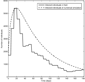
(a) Infectious with symptoms $I^{*}$

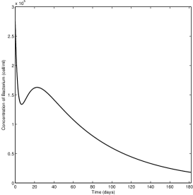
(b) Bacterial concentration $B^{*}$

Figure 1: Solutions $I^{*}$ and $B^{*}$ predicted by our model (21) with $\omega=\delta=\varepsilon=\alpha_{2}=0$ and the other parameter values as given in Table 1 versus real data from the cholera outbreak in the Department of Artibonite, Haiti, from $1$st November 2010 to $1$st May 2011 (solid line in (a)).

5.2 Local stability of the endemic equilibrium of the SIQRB model

For the parameter values in Table 1, we have that the basic reproduction number (7) is

$$R_{0}=8.2550$$

and the endemic equilibrium (9) is

$$E^{*}=(S^{*},I^{*},Q^{*},R^{*},B^{*})=(2684.3930,27.2540,6.8093,1217.7101,825.8793).$$

In Figure 2 we can observe agreement between the numerical simulation of the model (1) and the analysis of the local stability of the endemic equilibrium $E^{*}$ done in Section 3.2.

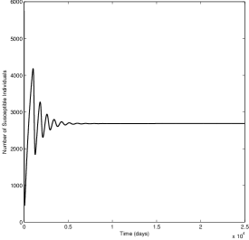
(a) Susceptible $S^{*}(t)$

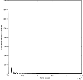
(b) Infectious with symptoms $I^{*}(t)$

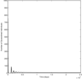
(c) In treatment through quarantine $Q^{*}(t)$

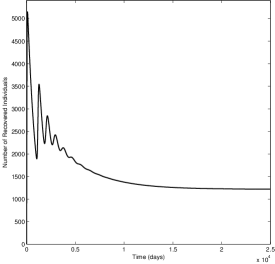
(d) Recovered $R^{*}(t)$

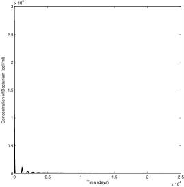
(e) Bacterial concentration $B^{*}(t)$

Figure 2: State trajectories of model (1) for the parameter values and initial conditions of Table 1.

5.3 Optimal control solution

We now solve the optimal control problem proposed in Section 4 for $W=2000$ [35] and the parameter values and initial conditions in Table 1.

Parameter	Description	Value	Reference
$\Lambda$	Recruitment rate	24.4$N(0)$/365000 (day-1)	[13]
$\mu$	Natural death rate	2.2493$\times 10^{-5}$ (day-1)	[14]
$\beta$	Ingestion rate	0.8 (day-1)	[2]
$\kappa$	Half saturation constant	$10^{6}$ (cell/ml)	[26]
$\omega$	Immunity waning rate	0.4/365 (day-1)	[22]
$\delta$	Quarantine rate	0.05 (day-1)	Assumed
$\varepsilon$	Recovery rate	0.2 (day-1)	[21]
$\alpha_{1}$	Death rate (infected)	0.015 (day-1)	[21]
$\alpha_{2}$	Death rate (quarantined)	0.0001 (day-1)	[21]
$\eta$	Shedding rate (infected)	10 (cell/ml day-1 person-1)	[2]
$d$	Bacteria death rate	0.33 (day-1)	[2]
$S(0)$	Susceptible individuals at $t=0$	5750 (person)	Assumed
$I(0)$	Infected individuals at $t=0$	1700 (person)	[33]
$Q(0)$	Quarantined individuals at $t=0$	0 (person)	Assumed
$R(0)$	Recovered individuals at $t=0$	0 (person)	Assumed
$B(0)$	Bacterial concentration at $t=0$	$275\times 10^{3}$ (cell/ml)	Assumed

Table 1: Parameter values and initial conditions for the SIQRB model (1).

The optimal control takes the maximum value for $t\in[0,87.36]$ days. For $t\in\ ]87.36,182]$, the optimal control is a decreasing function and at the final time we have $u^{\diamond}(182)\approx 0.00159$ (see Figure 3).

Figure 3: The optimal control (20) for the parameter values and initial conditions of Table 1.

At the end of approximately 88 days, the number of infectious individuals associated with the optimal control strategy decreases from 1700 to approximately 86 individuals and at the final time of $T=182$ days, the number of infectious individuals associated with the optimal control is, approximately, $23$ (see Figure 4a). We observe that the strategy associated with the control $u^{\diamond}$ allows an important decrease on the number of infectious individuals as well as on the concentration of bacteria. The maximum value of the number of infectious individuals also decreases significantly when the control strategy is applied. The optimal control implies a significant transfer of individuals to the recovered class.

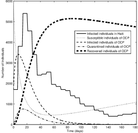
(a)

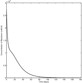
(b)

Figure 4: (a) In solid line: real data from the cholera outbreak in the Department of Artibonite, Haiti, from $1$st November 2010 to $1$st May 2011; in dashed lines the optimal solutions $S^{\diamond}$, $I^{\diamond}$, $Q^{\diamond}$ and $R^{\diamond}$ of the OCP (Optimal Control Problem) (14) with parameter values and initial conditions of Table 1. (b) Optimal bacterial concentration for the optimal control problem (14) with parameter values and initial conditions of Table 1.

6 Conclusion

SIR (Susceptible–Infectious–Recovered) type models and optimal control theory provide powerful tools to describe and control infection disease dynamics [16, 18, 29]. In this paper we propose a SIQRB model for cholera transmission dynamics. Our model differs from the other mathematical models for cholera dynamics transmission in the literature, because it assumes that infectious individuals subject to treatment stay in quarantine during that period. Our goal is to find the optimal way of using quarantine with the less possible cost and, simultaneously, to minimize the number of infectious individuals and the bacteria concentration. For that we propose an optimal control problem, which is analyzed both analytically and numerically. The numerical simulations show that after approximately three months ($87.36$ days) the optimal strategy implies a gradual reduction of the fraction of infectious individuals that stay in quarantine. To be precise, by introducing the optimal strategy through quarantine, as a way of systematizing treatment, one reduces the 2247 infected individuals reported by WHO in [33] (see Figure 1a) to just 86 infected individuals (see Figure 4a). Since quarantine implies a big economic, social and individual effort, it is important to know the instant of time from which the infectious individuals may leave quarantine without compromising the minimization of the number of infectious individuals and the bacterial concentration.

References

• [1] V. Capasso, S. L. Paveri-Fontana, A mathematical model for the 1973 cholera epidemic in the European Mediterranean region, Rev. Epidemiol. Sante 27 (1979), 121–132.
• [2] F. Capone, V. De Cataldis and R. De Luca, Influence of diffusion on the stability of equilibria in a reaction–diffusion system modeling cholera dynamic, J. Math. Biol. 71 (2015), 1107–1131.
• [3] J. Carr, Applications Centre Manifold Theory, Springer-Verlag, New York, 1981.
• [4] C. Castillo-Chavez and B. Song, Dynamical models of tuberculosis and their applications, Math. Biosc. Engrg. 1 (2004), 361–404.
• [5] Centers for Disease Control and Prevention, Quarantine and Isolation, 31 July 2014, http://www.cdc.gov/quarantine/historyquarantine.html.
• [6] L. Cesari, Optimization — Theory and Applications. Problems with Ordinary Differential Equations, Applications of Mathematics 17, Springer-Verlag, New York, 1983.
• [7] C. T. Codeco, Endemic and epidemic dynamics of cholera: the role of the aquatic reservoir, BMC Infect. Dis. 1(1) (2001), 14 pp.
• [8] R. Denysiuk, C. J. Silva, D. F. M. Torres, Multiobjective approach to optimal control for a tuberculosis model, Optim. Methods Softw. 30(5) (2015), 893–910. arXiv:1412.0528
• [9] W. H. Fleming, R. W. Rishel, Deterministic and Stochastic Optimal Control, Springer Verlag, New York, 1975.
• [10] D. M. Hartley, J. B. Morris, D. L. Smith, Hyperinfectivity: a critical element in the ability of V. cholerae to cause epidemics Plos Med. 3(1) (2006), e7, 63–69.
• [11] H. W. Hethcote, The mathematics of infectious diseases, SIAM Rev. 42 (2000), 599–653.
• [12] S. D. Hove-Musekwa, F. Nyabadza, C. Chiyaka, P. Das, A. Tripathi, Z. Mukandavire, Modelling and analysis of the effects of malnutrition in the spread of cholera, Math. Comput. Model. 53 (2010), 1583–1595.
• [13] Index Mundi, 30 June 2015, http://www.indexmundi.com/g/g.aspx?c=ha&v=25.
• [14] Index Mundi, 30 June 2015, http://www.indexmundi.com/g/g.aspx?c=ha&v=26.
• [15] R. I. Joh, H. Wang, H. Weiss, J. S. Weitza, Dynamics of indirectly transmitted infectious diseases with immunological threshold, Bull. Math. Biol. 71 (2009), 845–862.
• [16] B. W. Kooi, M. Aguiar, N. Stollenwerk, Bifurcation analysis of a family of multi-strain epidemiology models, J. Comput. Appl. Math. 252 (2013), 148–158.
• [17] S. Lenhart, J. T. Workman, Optimal control applied to biological models, Chapman & Hall/CRC Mathematical and Computational Biology Series, Chapman & Hall/CRC, Boca Raton, FL, 2007.
• [18] A. Mallela, S. Lenhart, N. K. Vaidya, HIV–TB co-infection treatment: Modeling and optimal control theory perspectives, J. Comput. Appl. Math. 307 (2016), 143–161.
• [19] J. Matovinovic, A short history of quarantine (Victor C. Vaughan), Univ. Mich. Med. Cent. J. 35 (1969), 224–228.
• [20] Z. Mukandavire, F. K. Mutasa, S. D. Hove-Musekwa, S. Dube, J. M. Tchuenche, Mathematical analysis of a cholera model with carriers and assessing the effects of treatment, In: Wilson, L.B. (Ed.), Mathematical Biology Research Trends. Nova Science Publishers (2008), pp. 1–37.
• [21] A. Mwasa, J. M. Tchuenche, Mathematical analysis of a cholera model with public health interventions, Bull. Math. Biol. 105 (2011), 190–200.
• [22] R. L. M. Neilan, E. Schaefer, H. Gaff, K. R. Fister, S. Lenhart, Modeling Optimal Intervention Strategies for Cholera, Bull. Math. Biol. 72 (2010), 2004–2018.
• [23] G. J. Olsder, J. W. van der Woude, Mathematical Systems Theory, VSSD, Delft, 2005.
• [24] M. Pascual, L. F. Chaves, B. Cash, X. Rodo, M. D. Yunus, Predicting endemic cholera: the role of climate variability and disease dynamics, Climate Res. 36 (2008), 131–140.
• [25] L. Pontryagin, V. Boltyanskii, R. Gramkrelidze, E. Mischenko, The Mathematical Theory of Optimal Processes, Wiley Interscience, 1962.
• [26] R. P. Sanches, C. P. Ferreira, R. A. Kraenkel, The Role of Immunity and Seasonality in Cholera Epidemics, Bull. Math. Biol. 73 (2011), 2916–2931.
• [27] Z. Shuai, J. H. Tien, P. van den Driessche, Cholera Models with Hyperinfectivity and Temporary Immunity, Bull. Math. Biol. 74 (2012), 2423–2445.
• [28] C. J. Silva, D. F. M. Torres, Optimal control for a tuberculosis model with reinfection and post-exposure interventions, Math. Biosci. 244 (2013), 154–164. arXiv:1305.2145
• [29] C. J. Silva, D. F. M. Torres, A TB-HIV/AIDS coinfection model and optimal control treatment, Discrete Contin. Dyn. Syst. 35 (2015), 4639–4663. arXiv:1501.03322
• [30] E. Tognotti, Lessons from the History of Quarantine, from Plague to Influenza A, Emerg. Infect. Dis. 19(2) (2013), 254–259.
• [31] D. F. M. Torres, Carathéodory equivalence Noether theorems, and Tonelli full-regularity in the calculus of variations and optimal control, J. Math. Sci. (N. Y.) 120(1) (2004), 1032–1050. arXiv:math/0206230
• [32] P. van den Driessche, J. Watmough, Reproduction numbers and subthreshold endemic equilibria for compartmental models of disease transmission, Math. Biosc. 180 (2002), 29–48.
• [33] World Health Organization, Global Task Force on Cholera Control, Cholera Country Profile: Haiti, 18 May 2011, http://www.who.int/cholera/countries/HaitiCountryProfileMay2011.pdf.
• [34] X. Yang, L. Chen, J. Chen, Permanence and positive periodic solution for the single-species nonautonomous delay diffusive models, Comput. Math. Appl. 32(4) (1996) 109–116.
• [35] M. G. West, The high cost of quarantine: Expenses range from police protection to takeout meals, The Wall Street Journal, Oct. 29, 2014. http://www.wsj.com/articles/the-high-cost-of-quarantine-and-who-pays-for-it-1414546114