Time-reversal and rotation symmetry breaking superconductivity in Dirac materials

Abstract

We consider mixed symmetry superconducting phases in Dirac materials in the odd parity channel, where pseudoscalar and vector order parameters can coexist due to their similar critical temperatures when attractive interactions are of finite range. We show that the coupling of these order parameters to unordered magnetic dopants favors the condensation of novel time-reversal symmetry breaking (TRSB) phases, characterized by a condensate magnetization, rotation symmetry breaking, and simultaneous ordering of the dopant moments. We find a rich phase diagram of mixed TRSB phases characterized by peculiar bulk quasiparticles, with Weyl nodes and nodal lines, and distinctive surface states. These findings are consistent with recent experiments on Nb_xBi₂Se₃ that report evidence of point nodes, nematicity, and TRSB superconductivity induced by Nb magnetic moments.

Introduction – One of the most fascinating aspects of unconventional superconductivity is that the condensate can display spontaneous time reversal symmetry breaking (TRSB), hosting an intrinsic Cooper pair magnetization Sigrist and Ueda (1991); Maeno et al. (1994). This can occur only with a multicomponent order parameter when the different components develop relative phases, as in the well known $p+ip$ chiral state proposed for Sr₂RuO₄ or the $d+id$ state conjectured for some cuprate superconductors Sigrist and Ueda (1991). Experimental evidence of TRSB superconductivity has been obtained from muon spin rotation $\mu$SR in UPt₃ Luke et al. (1993) and Sr₂RuO₄ Luke et al. (1998), from the polar Kerr effect Kapitulnik et al. (2009) and from Josephson tunneling experiments. The two-dimensional $p+ip$ state in particular has attracted great interest as a topological superconductor with protected edge and vortex modes, of potential use in the field of quantum computation Nayak et al. (2008); Qi and Zhang (2011). In a three dimensions chiral SC is also possible, allowing the realization of a Weyl superconductor with Majorana arcs on the surface Meng and Balents (2012); Sau and Tewari (2012); Yang et al. (2014), but realistic candidate materials for this superconducting state are lacking.

Recently, very compelling evidence for unconventional superconductivity has been reported in Dirac materials of the Bi₂Se₃ family upon doping Zhang et al. (2009); Hasan and Kane (2010); Qi and Zhang (2011). These studies were originally motivated by the prediction of a three dimensional, time- reversal invariant (TRI) topological superconductor featuring protected Andreev surface states Fu and Berg (2010). However, the rich phenomenology gathered so far suggests a more complicated pairing scenario. Superconductivity was first observed in Cu_xBi₂Se₃ Hor et al. (2010); Wray et al. (2010); Kriener et al. (2011), but evidence for the characteristic surface Andreev states has remained controversial  Sasaki et al. (2011); Levy et al. (2013); Peng et al. (2013). Moreover, nuclear magnetic resonance experiments  Matano et al. (2016) reveal that there is spin rotation symmetry breaking in the superconducting state, which rather supports a different pairing state of nematic type +  Fu (2014); Venderbos et al. (2016a). Superconductivity was also reported in Sr_xBi₂Se₃ Shruti et al. (2015); Liu et al. (2015) and in Tl_xBi₂Te₃ Wang et al. (2016), but evidence for unconventional pairing is lacking. Most interestingly, superconductivity has also been reported in Nb_xBi₂Se₃ Qiu et al. (2015), where initially paramagnetic samples were shown to develop a spontaneous magnetization at the superconducting transition. The magnetization survived only at the surface in the Meissner state, and it was claimed to originate from Nb magnetic moments. In the same compound, a later torque magnetometry experiment  Asaba et al. (2017) showed clear signatures of rotation symmetry breaking, and penetration depth measurements revealed a power law dependence with temperature Smylie et al. (2016) which points to the existence of nodes in the gap.

This complicated phenomenology is perhaps best understood within the minimal model of a superconducting Dirac Hamiltonian with approximate rotation symmetry, where there are only three possible pairing channels: a conventional $s$-wave scalar, an odd-parity pseudoscalar, and a vector. The pseudoscalar order parameter $\chi$ corresponds to the TRI topological superconductor, while rotation symmetry breaking can only be produced by the vector $\boldsymbol{\psi}$. The condensation of $\boldsymbol{\psi}$ is therefore a prerequisite to explain current experiments, but it has previously been shown that with only local interactions the $\chi$ channel always has a higher critical temperature than the $\boldsymbol{\psi}$ channel Fu and Berg (2010). In addition, even if $\chi$ could be ignored, $\boldsymbol{\psi}$ remains time-reversal symmetric within current models Fu (2014); Venderbos et al. (2016b). These two problems make the explanation of the observed phenomenology a theoretical challenge.

Motivated by the recent experiments, in this work we develop a theory of possible TRSB superconducting phases of doped Dirac Hamiltonians in the presence of magnetic impurities. We first show that when further neighbor electron-electron interactions are included, the critical temperature of $\boldsymbol{\psi}$ raises and can become comparable to that of $\chi$, providing a solution to the first problem. The closeness of the critical temperatures enables new mixed symmetry phases where both order parameters can condense simultaneously, similar to $s+id$ states predicted in high-T_c superconductors Kotliar (1988); Musaelian et al. (1996); Lee et al. (2009). We then develop a theory for these mixed phases, showing that the coupling of magnetic impurities, which would otherwise be paramagnetic, to the magnetization of the Cooper pairs Walker and Samokhin (2002); Mineev (2002); Samokhin and Walker (2002); MINEEV (2004) favors the condensation of TRSB phases and the consequent ordering of the magnetic impurities. We find three novel mixed TRSB phases that differ in the way rotation and gauge symmetries are broken and can be distinguished by their bulk spectrum, which may be gapped or feature Weyl nodes or nodal lines, or by the existence of surface states. We find a phase that is consistent with the surface magnetization Qiu et al. (2015), rotation symmetry breaking Asaba et al. (2017) and the existence of linear nodes Smylie et al. (2016).

Superconductivity in Dirac materials – We now consider the possible superconducting instabilities of Dirac Hamiltonians. To make contact with previous work, we start with the Hamiltonian commonly employed to describe Bi₂Se₃ Fu and Berg (2010)

$${\cal H}_{0}=m\sigma_{x}+v\sigma_{z}(k_{x}s_{y}-k_{y}s_{x})+v_{z}k_{z}\sigma_{y},$$ (1)

where $s_{i}$ are spin Pauli matrices and $\sigma_{i}$ are Pauli matrices for $p_{z}$-orbitals in the top and bottom layer of the quintuple layer QL Bi₂Se₃ structure, $v$ is the Fermi velocity, $m$ the insulating mass. The time reversal operator is ${\cal T}=is_{y}K$ with $K$ complex conjugation. When $v_{z}=v$, this Hamiltonian is a particular realization of the isotropic Dirac Hamiltonian of the form

$${\cal H}_{0}=\gamma_{0}m+v\gamma_{0}\gamma_{i}k_{i}$$ (2)

where the Euclidean gamma matrices $\gamma_{\mu}=(\gamma_{0},\gamma_{i})$ satisfy $[\gamma_{\mu},\gamma_{\nu}]_{+}=\mathcal{I}_{\mu\nu}$ and are given by $\gamma_{\mu}=(\sigma_{x},-\sigma_{y}s_{y},\sigma_{y}s_{x},\sigma_{z})$. In this work we will preferentially use the general Dirac matrices to emphasize the structure of the rotation group: $\gamma_{i}$ transforms as a vector, $\gamma_{0}$ as a scalar, and the matrix $\gamma_{5}\equiv\gamma_{0}\gamma_{1}\gamma_{2}\gamma_{3}$ as a pseudoscalar.

To classify the possible pairing channels, we introduce the Nambu spinor $\Psi_{\bf k}=({\bf c}^{\dagger}_{\bf k},is_{y}{\bf c}_{-{\bf k}})^{T}$, with ${\bf c}_{\bf k}$ fermionic annihilation operators of ${\cal H}_{0}$, and consider the Bogolyubov-deGennes Hamiltonian $\hat{H}=\frac{1}{2}\int d{\bf k}\Psi^{\dagger}_{\bf k}{\cal H}_{\bf k}\Psi_{\bf k}$, with

$${\cal H}_{\bf k}=({\cal H}_{0}({\bf k})-\mu)\tau_{z}+\Delta_{\bf k}\tau_{+}+\Delta^{\dagger}_{\bf k}\tau_{-},$$ (3)

where $\mu$ is the chemical potential, $\Delta_{\bf k}$ stands for generic momentum-dependent $4\times 4$ pairing matrices and $\tau_{i}$ Pauli matrices act in the particle-hole space. The Nambu construction imposes the charge conjugation symmetry ${\cal C}$ implemented as $U_{\cal C}{\cal H}(-{\bf k})^{*}U_{\cal C}^{\dagger}=-{\cal H}({\bf k})$, with $U_{\cal C}=s_{y}\tau_{y}$, which amounts to the restriction $s_{y}\Delta^{*}(-{\bf k})s_{y}=\Delta({\bf k})$. If pairing is momentum independent Fu and Berg (2010); Hashimoto et al. (2016), only six possible matrices in the Dirac algebra satisfy this constraint: the two even-parity scalars $I$ and $\gamma^{0}$, the pseudo-scalar $\gamma^{5}$ and the vector $\gamma^{i}$, which are both odd under parity. Disregarding the even-parity scalars, the pairing matrix takes the form $\Delta=\chi\gamma^{5}+\boldsymbol{\psi}\cdot\boldsymbol{\gamma}$. For the specific model of Bi₂Se₃, it was concluded that the local interorbital interaction $V$ can give rise to pairing in both of these channels, but the critical temperatures of the two channels satisfy $T_{\chi}\gg T_{\psi}$, Fu and Berg (2010), which makes it unlikely for the system to condense in the vector channel as stated previously.

We suggest that this problem can be solved by considering momentum-dependent corrections to the two-body interorbital density-density interaction. At lowest order in ${\bf q}={\bf k}-{\bf k}^{\prime}$ one has

$$V({\bf k},{\bf k}^{\prime})=V\left(1+a^{2}{\bf k}\cdot{\bf k}^{\prime}\right),$$ (4)

with $a$ a length scale on order of the lattice constant. In order to decouple the additional momentum-dependent interaction term we need to consider the other ten matrices in the Dirac algebra Sup . In particular, we note that that pairing matrix $\gamma^{5}\gamma^{i}k^{j}\epsilon_{ijk}$ is also a vector, and it modifies the gap matrix as

$$\Delta_{\bf k}=\chi\gamma^{5}+\boldsymbol{\psi}\cdot(\boldsymbol{\gamma}-ia\gamma^{5}\boldsymbol{\gamma}\times{\bf k}).$$ (5)

It is instructive to project the $4\times 4$ Dirac matrices into the $2\times 2$ space of the Kramers degenerate conduction band states relevant to pairing Venderbos et al. (2016b). If we define Pauli matrices $\tilde{s}_{i}$ for this space, the gap matrix takes the form $\Delta_{\bf k}=\chi\tilde{\bf k}\cdot\tilde{\bf s}+\boldsymbol{\psi}\times\tilde{\bf k}\cdot\tilde{\bf s}(1+\mu a/v)$, with $\tilde{\bf k}=v{\bf k}/\mu$. Thus, while seemingly of higher order in the Dirac Hamiltonian, the correction term is actually of the same order when projected to the Fermi surface. The momentum dependence of the pairing interaction affects only the vector channel and it raises its critical temperature $T_{\psi}$, which becomes comparable to $T_{\chi}$ Sup .

Ginzburg-Landau free energy – We now consider superconductivity at the level of the Ginzburg-Landau (GL) free energy. The pseudoscalar order parameter free energy is

$$F_{\chi}=a_{1}|\chi|^{2}+b_{1}|\chi|^{4}$$ (6)

and condensation of $\chi$ takes place when $a_{1}(T_{\chi})=0$. For the vector order parameter $\boldsymbol{\psi}$, symmetry dictates that the form of the free energy be Ueda and Rice (1985); Knigavko and Rosenstein (1999)

$$F_{\psi}=a_{2}|\boldsymbol{\psi}|^{2}+b_{2}|\boldsymbol{\psi}|^{4}+b_{2}^{\prime}|\boldsymbol{\psi}\times\boldsymbol{\psi}^{*}|^{2}.$$ (7)

The vector representation admits two possible superconducting states: a nematic state $\boldsymbol{\psi}\propto(1,0,0)$ which is time-reversal invariant, and a chiral TRSB state $\boldsymbol{\psi}\propto(1,\pm i,0)$ Fu (2014); Venderbos et al. (2016b). The sign of the coupling $b_{2}^{\prime}$ determines whether the vector representation chooses the nematic (for $b_{2}^{\prime}>0$) or the chiral state (for $b_{2}^{\prime}<0$). Since at second order no coupling is allowed by symmetry between $\chi$ and $\boldsymbol{\psi}$, the condensation of $\boldsymbol{\psi}$ takes place when $a_{2}(T_{\psi})=0$. However, our previous argument suggesting that $a_{1}\sim a_{2}$ Sup and $T_{\chi}\sim T_{\psi}$ require that we study a coupled theory beyond second order where both order parameters may coexist. At fourth order the coupling term in the GL free energy reads,

$$F_{\psi,\chi}=d_{1}|\chi|^{2}|\boldsymbol{\psi}|^{2}+d_{2}\left|\chi^{*}\boldsymbol{\psi}-\chi\boldsymbol{\psi}^{*}\right|^{2},$$ (8)

and the total free energy is

$$F = F_{\chi}+F_{\psi}+F_{\chi,\psi}.$$ (9)

In the weak coupling regime with $a_{1}\sim a_{2}$ both order parameters acquire a finite value.

The possible TRSB phases arising from this free energy are characterized by a magnetization of the condensate, due to the spin triplet state of the Cooper pairs. By symmetry, the magnetization must be built with gauge invariant combinations of order parameters and transform as a spin, i.e. as a ${\cal T}$-odd pseudo-vector (even under inversion). Since $\boldsymbol{\psi}$ is a vector and $\chi$ a pseudoscalar, the following combinations satisfy the symmetry requirements,

$$\boldsymbol{\Sigma}_{1}=\chi\boldsymbol{\psi}^{*}-\chi^{*}\boldsymbol{\psi},\qquad\boldsymbol{\Sigma}_{2}=\boldsymbol{\psi}\times\boldsymbol{\psi}^{*}.$$

Note that $\boldsymbol{\Sigma}_{1}$ cannot be built with a standard $s$-wave order parameter because the combination would not be a pseudovector. These two pseudovectors are orthogonal and appear quadratically in the GL Eqs. (7, 8).

The different possible phases obtained from the GL free energy Eq. (9) are realized with different signs of the interaction parameters $b_{2}^{\prime}$ and $d_{2}$ and can be distinguished by the values of ${\bf\Sigma}_{1}$ and ${\bf\Sigma}_{2}$ and the way rotation and gauge symmetries are broken. For $d_{2},b_{2}^{\prime}>0$ one has ${\bf\Sigma}_{1}={\bf\Sigma}_{2}=0$ and the system is in the TRI nematic phase, with rotation symmetry about the nematic director. When $d_{2}<0$ and $b_{2}^{\prime}>0$ one has ${\bf\Sigma}_{1}\neq 0$ and ${\bf\Sigma}_{2}=0$, and the system is invariant under rotations about ${\bf\Sigma}_{1}$. We name this phase TRSB 1. When $d_{2},b_{2}^{\prime}<0$ one has ${\bf\Sigma}_{2}\neq 0$, and the system is in the chiral phase, with $\boldsymbol{\psi}\propto(1,i,0)$. In this case the system is invariant under rotations around ${\bf\Sigma}_{2}$ combined with a gauge transformation Sup . Finally, when $d_{2}>0$ and $b_{2}^{\prime}<0$ one has ${\bf\Sigma}_{2}\neq 0$, but $\boldsymbol{\psi}$ is not in the purely chiral state, but rather in a hybrid solution Sup which has no symmetry. We name this phase TRSB 2.

A schematic phase diagram as a function of $b_{2}^{\prime}$ and $d_{2}$ is depicted in Fig. 1. Microscopic calculations Fu (2014); Venderbos et al. (2016b); Sup show that for an isotropic model $b_{2}^{\prime},d_{2}>0$, precluding a TRSB phase. We show next how a coupling to magnetic dopants renormalizes the coefficients $b_{2}^{\prime}$ and $d_{2}$ and can change their sign if the coupling is strong enough.

Coupling to dopant magnetization – The presence of random magnetic moments in the sample can be described by an average magnetization ${\bf M}$. At the Landau theory level, both ${\bf\Sigma}_{1}$ and ${\bf\Sigma}_{2}$ can couple linearly to ${\bf M}$ Walker and Samokhin (2002); Mineev (2002); Samokhin and Walker (2002); MINEEV (2004) which is also a ${\cal T}$-odd pseudo-vector

$$F_{\chi,\psi,M}=i{\bf M}\cdot[c_{1}(\chi\boldsymbol{\psi}^{*}-\chi^{*}\boldsymbol{\psi})+c_{2}\boldsymbol{\psi}\times\boldsymbol{\psi}^{*}].$$ (10)

By appropriately aligning ${\bf M}$, we see that the system may lower its energy by condensing in a TRSB phase with finite condensate magnetizations.

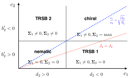
Figure 1: Phase diagram of superconductivity involving the pseudo-scalar and the vector order parameters coupled to the dopants magnetization. The four possible phases can be obtained by properly tuning the couplings $J_{1}$ and $J_{2}$.

Neglecting interactions between the magnetic moments, the full free energy at second order in ${\bf M}$ including the superconducting order parameters reads

$$F=a_{3}|{\bf M}|^{2}+F_{\chi}+F_{\psi}+F_{\chi,\psi}+F_{\chi,\psi,M}.$$ (11)

Since the dopants are paramagnetic above $T_{c}$, we assume $a_{3}>0$. The mean-field solution for ${\bf M}$ can be found by minimizing the free energy with respect to ${\bf M}$, finding ${\bf M}=-i\frac{c_{1}}{2a_{3}}{\bf\Sigma}_{1}-i\frac{c_{2}}{2a_{3}}{\bf\Sigma}_{2}$. It is clear that a non-zero magnetization ${\bf M}$ arises in all TRSB phases, despite the fact that the dopants are initially paramagnetic. Substituting the mean-field value of the magnetization the free energy takes the form of Eq. (9) with modified parameters

$$d_{2}\to d_{2}-\frac{c_{1}^{2}}{4a_{3}},\qquad b_{2}^{\prime}\to b_{2}^{\prime}-\frac{c^{2}_{2}}{4a_{3}}.$$ (12)

Since the coupling to magnetic dopants renormalizes both $b_{2}^{\prime}$ and $d_{2}$, with different values of $c_{1}$ and $c_{2}$ one can now span the entire phase diagram in Fig. 1.

Meissner screening - The presence of the magnetic dopants induces the condensation of a TRSB phase where the dopants moments are aligned with the spin magnetization of the condensate. The resulting total spin magnetization ${\bf M}_{\rm s}={\bf M}+i\mu({\bf\Sigma}_{1}+{\bf\Sigma}_{2})$ acts back onto the orbital degrees of freedom and the GL free energy is Ginzburg (1957); Shopova and Uzunov (2005)

$${\cal F}=\int d{\bf r}~{}\left[F+\frac{{\bf B}^{2}}{8\pi}-{\bf B}\cdot{\bf M}_{\rm s}+F^{\rm grad}_{\chi,\boldsymbol{\psi},{\bf M}}\right].$$ (13)

where ${\bf B}$ is the full induction field and $F^{\rm grad}$ accounts for gradient terms for the order parameters Sup . For finite ${\bf M}_{\rm s}$ the system may develop screening supercurrents, so that ${\bf B}={\bf H}+4\pi({\bf M}_{\rm s}+{\bf M}_{\rm o})$, with ${\bf M}_{\rm o}$ the orbital magnetization due to screening currents, and ${\bf H}$ an external field. For ${\bf H}=0$, the order parameters in the bulk can be taken to be constant, so that ${\bf B}=0$ by Meissner screening, provided that $M_{\rm s}<H_{\rm cr}$, with $H_{\rm cr}$ the thermodynamic critical field Ginzburg (1957); Sup . Since $M_{\rm s}$ is linked to the mean-field value of $\chi$ and $\boldsymbol{\psi}$, for $a_{1}\sim a_{2}$ the ratio $M_{\rm s}/H_{\rm cr}$ is temperature independent and it is suppressed by strong $b_{1}$ and $b_{2}$. At the surface of the system the cancelation between spin and orbital magnetization is not satisfied locally, due to difference in the coherence length, penetration depth, and the length scale of variation of ${\bf M}$, and a finite surface magnetization may arise, in agreement with the observations of Ref. Qiu et al. (2015).

Microscopic coupling – The coupling Eq. (10) and the resulting phase diagram is generic of a SO(3) invariant theory. The only symmetry allowed microscopic coupling must be written in terms of the spin pseudovectors ${\bf S}_{\parallel}\equiv(s_{x},s_{y},\sigma_{x}s_{z})$ and ${\bf S}_{\perp}\equiv(\sigma_{x}s_{x},\sigma_{x}s_{y},s_{z})$ Sup ,

$$H_{\rm Z}=J_{1}{\bf M}\cdot{\bf S}_{\parallel}+J_{2}{\bf M}\cdot{\bf S}_{\perp}.$$ (14)

The coefficients $c_{1}$ and $c_{2}$ can be derived microscopically from this coupling, and doing so reveals the constraint $c_{1}(J_{1}m/\mu+J_{2})=2c_{2}(J_{1}+J_{2}m/\mu)$ Sup . All phases in Fig. 1 can therefore be realized by properly tuning $J_{1}$, $J_{2}$, and $m/\mu$. In Bi₂Se₃, the SO(3) symmetry breaks down to the lattice point group $D_{3d}$ when anisotropy corrections are included Fu and Berg (2010). The vector $\boldsymbol{\psi}=(\psi_{x},\psi_{y},\psi_{z})$ splits into a two-component $E_{u}\sim(-\psi_{y},\psi_{x})$ and one-component $A_{2u}\sim\psi_{z}$ representations. The pseudoscalar $\chi$ corresponds to the $A_{1u}$ representation. A microscopic coupling between the magnetic moments and the physical spin ${\bf s}$ of the electrons in Bi₂Se₃ can be written in terms of a Zeeman coupling $H_{\rm Z}=-J(s_{x}M_{x}+s_{y}M_{y})-J_{z}s_{z}M_{z}$ with $J\neq J_{z}$ anisotropic Zeeman coupling constants. The resulting phase diagram remains qualitatively very similar to the SO(3) invariant one Sup .

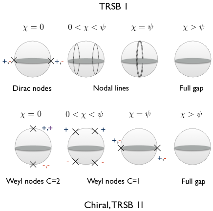
Figure 2: Schematics of the gap structure on the Fermi surface: TRSB 1 has Dirac nodes that evolve in nodal line for $\chi>0$. TRSB 2 and the chiral phase have Weyl points with $C=2$ that split in two $C=1$ upon switching $\chi$. The phases are fully gapped for $\chi>\psi$.

Gap structure – The value of the superconducting gap on the Fermi surface for the different phases depends on the relative strength of the two order parameters. When $\chi$ dominates all phases are fully gapped, but different cases arise if $\boldsymbol{\psi}$ dominates. In the nematic case the gap has Dirac nodes along the nematic direction for $\chi=0$. These nodes can be gapped by a small $\chi$ or by hexagonal warping terms Fu (2014), so that in general the phase is fully gapped. In the TRSB 1 phase the order parameters may be taken as $\boldsymbol{\psi}=\psi_{0}(1,0,0)$ and $\chi=\chi_{0}e^{i\gamma}$ and that the Dirac nodes for $\chi=0$ can be shown to become circular nodal lines defined by $\sin\theta=\pm\chi_{0}/\psi_{0}$, with $\theta$ the polar angle with respect to $\boldsymbol{\Sigma}_{1}$. Nodal lines of the north and south hemisphere join for $\chi=\psi$ and become gapped for $\chi>\psi$ (see Fig. 2). These nodal lines have a linear density of states (DOS) $\rho(\epsilon)\propto\epsilon$ Phillips and Aji (2014). In the chiral and the TRSB 2 phase a Weyl superconductor is realized Meng and Balents (2012); Sau and Tewari (2012); Yang et al. (2014); Venderbos et al. (2016b). For $\chi=0$ there are Weyl nodes of topological charge $C=\pm 2$ on the north and south pole along the direction of ${\bf\Sigma}_{2}$ Kozii et al. (2016). For finite $\chi$ these nodes are split into two Weyl nodes of $C=1$ at a finite polar angle and in the azimuthal direction given by $\Sigma_{1}$ and by increasing $\chi$ they move towards the equator where they meet with the nodes from the south hemisphere and gap out for $\chi>\psi$ (see Fig. 2). Note that while the DOS is linear in energy when $\chi=0$, $\rho_{C=2}(\epsilon)\propto\epsilon$, it becomes quadratic for finite $\chi$, $\rho_{C=1}(\epsilon)\propto\epsilon^{2}$ Fang et al. (2012). These predictions could be confirmed by STM or specific heat measurements. On the surface of Weyl superconductor there are Majorana arcs of different kinds Kozii et al. (2016), while in the gapped phases the topologically protected surface Andreev states associated to $\chi$ are gapped on the surfaces orthogonal to ${\bf\Sigma}_{1}$.

Discussion and conclusions– The features of the TRSB2 phase predicted in this work are consistent with all the observations made in recent experiments with Nb_xBi₂Se₃: the breaking of rotation Asaba et al. (2017) and time-reversal symmetry Qiu et al. (2015) and the presence of point nodes Smylie et al. (2016). These conclusions remain valid also if the scalar and vector representations are split due lattice symmetries. In this case, the lattice will naturally pin the direction of $\Sigma_{2}$ to the $c$ axis, while $\Sigma_{1}$ will lay in-plane, pointing in a high-symmetry direction. This is enough to reproduce the twofold pattern observed in torque magnetometry. Our work makes the additional prediction that the magnetization, which can only be observed in the surface due to Meissner screening, must have both in-plane and out-of-plane components. The TRSB2 phase also features linear nodes in the bulk with Chern number $C=1$, consistent with the scaling of the penetration depth. This is in contrast with the TRI nematic candidate state, which was argued to be fully gapped in the presence of trigonal warping Fu (2014). Our work further predicts the positions of the nodes to lie in the direction of $\Sigma_{1}$, a prediction that could be tested, for example, with the nodal spectroscopy techniques proposed in Refs. Stojković and Valls (1995); Žutić and Valls (1997); Halterman and Valls (2000). Finally, our work also provides a general framework to address current and future experiments with doped Dirac materials, emphasizing the importance of mixed symmetry states and coexistence of order parameters.

Note – During the preparation of this manuscript, we became aware of Ref. Yuan et al. (2017), where magnetic Nb dopants are also considered as the mechanism that stabilizes chiral superconductivity. This work does not provide a mechanism for the vector channel to compete with the pseudoscalar, and no mixed symmetry phases are considered. The chiral state proposed in Ref. Yuan et al. (2017) respects $C_{3}$ rotation symmetry, in contrast with Ref. Asaba et al. (2017). The issue of Meissner screening is also not addressed.

Acknowledgements – The authors acknowledge useful discussions with Irina Grigorieva. The authors acknowledge funding from the European Union’s Seventh Framework Programme (FP7/2007-2013) through the ERC Advanced Grant NOVGRAPHENE through grant agreement Nr. 290846 (L. C., F. J. and F. G.), from the Marie Curie Programme under EC Grant agreement No. 705968 (F. J.) and from the European Commission under the Graphene Flagship, contract CNECTICT-604391 (F. G.).

Appendix A Character on the Fermi surface: Dirac nodes, Weyl nodes, Majorana nodes

The four different phases that appear in the phase diagram of the pseudoscalar and vector order parameters coupled to a magnetization order parameter have a peculiar character on the Fermi surface. By writing the gap matrix as $\Delta={\bf d}_{\bf k}\cdot{\bf s}$, the character on the Fermi surface can be addressed by studying the bulk spectrum

$$E_{\pm}({\bf k})=\sqrt{(\epsilon_{\bf k}-\mu)^{2}+|{\bf d}_{\bf k}|^{2}\pm|{\bf d}_{\bf k}\times{\bf d}^{*}_{\bf k}|},$$ (15)

on the Fermi surface $\epsilon_{\bf k}=\mu$. With the vector ${\bf d}_{\bf k}=\chi{\bf k}+\boldsymbol{\psi}\times{\bf k}$ one can write the gap in terms of the condensate magnetization ${\bf\Sigma}_{1}$ and ${\bf\Sigma}_{2}$ as

$$\Delta_{\pm}({\bf k})=\sqrt{(|\chi|^{2}+|\boldsymbol{\psi}|^{2})k^{2}-|\boldsymbol{\psi}\cdot{\bf k}|^{2}\pm k\sqrt{|{\bf\Sigma}_{1}|^{2}k^{2}-|{\bf\Sigma}_{1}\cdot{\bf k}|^{2}+|{\bf\Sigma}_{2}\cdot{\bf k}|^{2}}},$$ (16)

with ${\bf k}$ on the Fermi surface, $k=1$. For $\boldsymbol{\psi}=0$ the phase is fully gapped, with $\Delta_{\pm}=|\chi|$

A.0.1 Nematic state

In the nematic phase one has $\chi$ and $\boldsymbol{\psi}$ both real, so that ${\bf\Sigma}_{1}={\bf\Sigma}_{2}=0$, and the gap reads

$$\Delta^{\rm nem}_{\pm}({\bf k})=\sqrt{|\chi|^{2}+|\boldsymbol{\psi}|^{2}-|\boldsymbol{\psi}\cdot\hat{\bf k}|^{2}},$$ (17)

so that the phase is fully gapped as long as $\chi\neq 0$, whereas for $\chi=0$ it has a two double degenerate nodes for $\hat{\bf k}\parallel\boldsymbol{\psi}$. These nodes represent Dirac points and can be gapped by hexagonal warping Fu (2014).

A.0.2 Chiral state

In the chiral phase one has $\chi$ real and $\boldsymbol{\psi}=\psi({\bf u}+i{\bf v})$, with ${\bf u}$ and ${\bf v}$ orthogonal unit vectors. Let us first consider the case $\chi=0$. The gap then reads

$$\Delta_{\pm}({\bf k})=\sqrt{|\boldsymbol{\psi}|^{2}-|\boldsymbol{\psi}\cdot{\bf k}|^{2}\pm|{\bf\Sigma}_{2}\cdot{\bf k}|},$$ (18)

It is clear that only the gap $\Delta_{-}$ can be zero on a given point $(\theta,\phi)$ of the Fermi surface. Due to SO(3) symmetry we can choose for simplicity $\boldsymbol{\psi}=\psi(1,i,0)$, so that by writing $\hat{\bf k}=(\sin\theta\cos\phi,\sin\theta\sin\phi,\cos\theta)$ the gap reads

$$\Delta^{\rm chi}_{\pm}({\bf k})\propto\psi(1\pm|\cos(\theta)|).$$ (19)

One has a node on the north pole $\theta=0$ and a node on the south pole $\theta=\pi$ on the Fermi sphere. Each node represents a Weyl point with topological charge $C=\pm 2$, with $C=+2$ at the north pole and $C=-2$ at the south pole. These nodes cannot be gapped unless nodes with opposite topological charge are brought into contact.

We can see this in more details by expanding the Hamiltonian in the reduced subspace of the conduction band for small momentum ${\bf q}$ around the the nodal points. For $\chi=0$ these are the north and south pole ${\bf k}^{\pm}_{F}=(0,0,\pm k_{F})$, and the Hamiltonian reads

$$H^{\rm chi}_{\pm,{\bf q}}=\left[\begin{array}[]{cccc}\pm v_{F}q_{z}&0&-i\psi q_{+}&\pm 2i\psi k_{F}\\ 0&\pm v_{F}q_{z}&0&i\psi q_{+}\\ i\psi q_{-}&0&\mp v_{F}q_{z}&0\\ \mp 2i\psi k_{F}&-i\psi q_{-}&0&\mp v_{F}q_{z}\end{array}\right],$$ (20)

where $q_{\pm}=q_{x}\pm iq_{y}$. We see that the Hamiltonian splits into two Weyl sub-blocks coupled by a mass term $m=2\psi k_{F}$ and the resulting eigenvalues give rise to two gapped bands at $\pm m$ and two gapless bands. Projecting onto the gapless states we find

$$h^{\rm chi}_{\pm,{\bf q}}=\pm\left[v_{F}q_{z}\sigma_{z}-\frac{\psi^{2}}{m}(iq_{+}^{2}\sigma_{+}-iq_{-}^{2}\sigma_{-})\right],$$ (21)

that is linearly dispersing along $q_{z}$ but quadratically dispersing along $q_{x}$ and $q_{y}$. One can show that the topological charge of these band crossing is $C=\pm 2$.

When $\chi\neq 0$ the gap reads

$$\Delta^{\rm chi}_{\pm}({\bf k})\propto\psi\sqrt{(\chi/\psi)^{2}+1+\cos^{2}(\theta)\pm 2\sqrt{\cos^{2}(\theta)((\chi/\psi)^{2}+1)+(\chi/\psi)^{2}\cos^{2}(\phi)\sin^{2}(\theta)}}.$$ (22)

One can look for nodal solutions of $\Delta_{-}$, that reduces to solve $\cos^{2}\theta_{W}=1-(\chi/\psi)^{2}e^{\pm 2i\phi}$, and find the there exist Weyl nodes with topological charge $|C|=1$ for $0<\chi<\psi$ only for $\phi=0,\pi$. The Weyl node with topological charge 2 is separated into two Weyl nodes with topological charge $C=1$ at finite angles $\pm\theta_{W}$ in the $x,z$ plane ($\phi=0$), and analogously for the nodes at the south pole. The quadratic crossing splits into two linear crossing with $C=1$ in the north hemisphere and two linear crossing with $C=-1$ in the north hemisphere It follows that by increasing $\chi$ one moves the Weyl nodes toward the equator and for $\chi=\psi$ one has that Weyl nodes of opposite charge are brought into contact and split, so that for $\chi>\psi$ the system is fully gapped.

In the plane $\phi=0$ the nodes are located at $\sin\theta_{W}=\pm\chi/\psi$. We expand the Hamiltonian around the point $\hat{\bf k}_{F}=(\sin\theta_{W},0,\cos\theta_{W})$, and define radial and tangential momentum ${\bf q}=(q_{\parallel,x},q_{\parallel,y},q_{\perp})$,

A.0.3 TRSB 1 state

In the TRSB phase 1 characterized by ${\bf\Sigma}_{1}\neq 0$ and ${\bf\Sigma}_{2}=0$ and one has $\chi$ real and $\boldsymbol{\psi}=i\psi{\bf n}$, with ${\bf n}$ a real unit vector. The gap reads

$$\Delta_{\pm}({\bf k})=\sqrt{(|\chi|^{2}+|\boldsymbol{\psi}|^{2})-|\boldsymbol{\psi}\cdot\hat{\bf k}|^{2}\pm\sqrt{|{\bf\Sigma}_{1}|^{2}-|{\bf\Sigma}_{1}\cdot\hat{\bf k}|^{2}}},$$ (23)

Choosing ${\bf n}=(1,0,0)$ the gap then reads

$$\Delta_{\pm}^{\rm TRSB1}\propto\left|\chi\pm\psi\sqrt{1-\sin^{2}(\theta)\cos^{2}(\phi)}\right|.$$ (24)

For $\chi=0$ one obtain Dirac nodes at $\theta=\pi/2$, $\phi=0,\pi$ as for the nematic case. For $0<\chi<\psi$ one has nodal lines. These are best seen by choosing the coordinate in momentum space so to align the $z$ direction to the nematic director (that is by choosing ${\bf n}=(0,0,1)$) so that the gap reads

$$\Delta_{\pm}^{\rm TRSB1}\propto\left|\chi\pm\psi\sin(\theta^{\prime})\right|,$$ (25)

with $\theta^{\prime}$ the polar angle with respect to the $x$ axis. It is then clear that the Dirac point at $\chi=0$ evolves in a circle.

A.0.4 TRSB 2 state

Finally we now address the character on the Fermi surface of the gap in the TRSB 2 phase, where both ${\bf\Sigma}_{1}$ and ${\bf\Sigma}_{2}$ are non-zero but with ${\bf\Sigma}_{2}$ not maximal. In this case one can in general write $\boldsymbol{\psi}=(\cos(\alpha/2),i\sin(\alpha/2),0)$ and take $\chi$ real. The gap function in this case is not particularly enlightening. Nevertheless, one can show that for $0<\chi<\psi$ in general one has 2 Weyl points of topological charge $C=1$ in the north hemisphere and 2 Weyl points of topological charge $C=-1$ negative in the south hemisphere. As in the purely chiral state the $\chi$ component moves the position of the Weyl points toward the equator and at $\chi=\psi$ they merge and split, so that for $\chi>\psi$ the state is gapped.

Appendix B Thermodynamic critical field in the TRSB phases

As we pointed out in the main text, a crucial point for the existence of a TRSB phase with a non-zero condensate a dopants spin magnetization is that the total spin magnetization $M_{\rm s}$ be smaller than the thermodynamic critical field, $M_{\rm s}<H_{\rm cr}$. The latter can be calculated by the condensation energy, that is the free energy evaluated in the minimum at the mean-field value of the order parameters. The case of the condensation of the vector order parameter only is particularly simple and the value of the thermodynamic field has a simple form that allows us to study the condition for TRSB. We present here the derivation of the ratio $M_{\rm s}/H_{\rm cr}$ for this particular case and results may be extended straightforwardly for the other TRSB phases presented in the main text.

It is rather reasonable to assume the coupling $c_{2}<0$, according to which the dopants and condensate spin magnetization tend to align along a given direction. The GL free energy then reads

$$F=a_{3}M^{2}+a_{2}\psi^{2}+(b_{2}+b_{2}^{\prime})\psi^{4}+c_{2}M\psi^{2},$$ (26)

where $\psi>0$ is the absolute value of the condensate order parameter and $M$ the absolute value of the dopants magnetization. At the minimum one has $M_{0}=-\frac{c_{2}}{2a_{3}}\psi_{0}^{2}$, that is positive under the assumption of $a_{3}>0$ and $c_{2}<0$, and $\psi_{0}^{2}=-2a_{2}a_{3}/(4a_{3}(b_{2}+b_{2}^{\prime})-c^{2}_{2})$, that is positive under the assumption that $a_{2}<0$ and $4a_{3}(b_{2}+b_{2}^{\prime})-c^{2}_{2}>0$. These two condition are essential for the stability of the superconducting phase described by a GL free energy up to forth order. The thermodynamic critical field is then given by

$$H_{\rm cr}=\sqrt{-8\pi F[M_{0},\psi_{0}]}.$$ (27)

Analogously, the value of the total spin magnetization is written as $M_{\rm s}=M_{0}+\mu\Sigma_{2}=(-\frac{c_{2}}{2a_{3}}+\mu)\psi_{0}^{2}$. The ratio between the the total spin magnetization and the critical field is then written as

$$\frac{M_{\rm s}}{H_{\rm cr}}=\sqrt{\frac{a_{3}}{2\pi}}\frac{\mu-c_{2}/(2a_{3})}{\sqrt{4a_{3}(b_{2}+b_{2}^{\prime})-c_{2}^{2}}}.$$ (28)

For a paramagnetic system $a_{3}>0$ is temperature independent in the range of temperature of interest and we have that $M_{\rm s}/H_{\rm cr}$ is temperature independent. Furthermore, a stable superconducting phase is stabilized by a large $b_{2}$, so that the ratio $M_{\rm s}/H_{\rm cr}$ is smaller than one for sufficiently large $b_{2}$.

Appendix C Microscopic Theory of Superconductivity in Bi₂Se₃

In the main text we studied superconductivity in the odd parity channel for a SO(3) Dirac Hamiltonian and we referred to Bi₂Se₃ as a possible material system. The Bi₂Se₃ family is well described by the 3D massive Dirac equation Eq. (1) that, with the construction of the Dirac matrices in terms of spin ${\bf s}$ and $p_{z}$ orbital $\boldsymbol{\sigma}$ Pauli matrices given in Table 1, can be casted in the form of a Dirac Hamiltonian. The actual point group of the material is $D_{3d}$ and we now specify to this case.

We now consider the full interacting problem described by purely interlayer interaction, since it is assumed that they play a major role. We go a step beyond the purely local interaction discussed in Ref. Fu and Berg (2010) and extend the attraction to nearest neighbors. In the Cooper channel the interaction reads

$$H_{\rm int}=-\frac{1}{2}\sum_{i\neq j}\sum_{{\bf k},{\bf k}^{\prime};s,s^{\prime}}V({\bf k}-{\bf k}^{\prime})c^{\dagger}_{{\bf k},i,s}c^{\dagger}_{-{\bf k},j,s^{\prime}}c_{-{\bf k}^{\prime},j,s^{\prime}}c_{{\bf k}^{\prime},i,s},$$ (29)

with $V({\bf q})$ the Fourier transform of the interaction potential. A detailed microscopic description of the nearest neighbor interaction in Bi₂Se₃ is beyond the scope of the present work and we simply assume that an expansion at lowest order in ${\bf q}={\bf k}-{\bf k}^{\prime}$ can be done. We take into account the anisotropy along the $z$-direction typical of the material by splitting the momentum as ${\bf k}=({\bf k}_{\parallel},k_{z})$ and introducing effective length scales $a$ and $a_{z}$ on order of the lattice constants. Defining ${\bf k}=({\bf k}_{\parallel},k_{z})$ the interaction reads

$$V({\bf k},{\bf k}^{\prime})=\frac{V}{2}\left(1+a^{2}{\bf k}_{\parallel}\cdot{\bf k}^{\prime}_{\parallel}+a_{z}^{2}k_{z}k_{z}^{\prime}\right).$$ (30)

These terms can involve only vectorial representations and tends to increase the strength of channel interaction. The next step consists in expanding the interaction in irreducible representations of the point group $D_{3d}$. When SO(3) is broken down to $D_{3d}$ the vector order parameter splits as $\boldsymbol{\psi}\to(\boldsymbol{\psi}_{\parallel},\psi_{z})$ and we can define the following basis functions

$$\Gamma_{x}^{1}({\bf k}) = -i\gamma^{5}\gamma^{2}k_{z},\qquad\Gamma_{x}^{2}({\bf k})=-i\gamma^{5}\gamma^{3}k_{y},$$ (31)

$$\Gamma_{y}^{1}({\bf k}) = -i\gamma^{5}\gamma^{3}k_{x},\qquad\Gamma_{y}^{2}({\bf k})=-i\gamma^{5}\gamma^{1}k_{z},$$

$$\Gamma_{z}({\bf k}) = -i\gamma^{5}(\gamma^{1}k_{y}-\gamma^{2}k_{x}),$$

where $\Gamma_{x}^{1,2}$ and $\Gamma_{y}^{1,2}$ belong to $E_{u}$ and $\Gamma_{z}$ belongs to $A_{2u}$. Following Sigrist and Ueda (1991) and focusing on the odd-parity sector we write the gap matrix as

$$\hat{\Delta}=\chi\gamma^{5}+\boldsymbol{\psi}\cdot\boldsymbol{\gamma}+a\psi_{z}F_{y}+\psi_{x}(a_{z}F_{x}^{1}-aF_{x}^{2})++\psi_{y}(aF_{y}^{1}-a_{z}F_{y}^{2}),$$ (32)

with both the pseudo-scalar $\chi$ and the vector $\boldsymbol{\psi}$ order parameters. We see that the extra terms contains the contraction of the momentum with the pseudo-vector $\gamma^{5}\boldsymbol{\gamma}$, that is the possible odd-parity term involving the momentum only allowed by symmetry, as explained in the next section. Setting the chemical potential in the conduction band, $\mu>m$, upon projecting onto the conduction band, one obtains the gap matrix

$$\Delta_{\bf k}=\chi\tilde{\bf k}\cdot\tilde{\bf s}+\boldsymbol{\psi}\times\tilde{\bf k}\cdot\tilde{\bf s}(1+\mu a/v)$$ (33)

for the isotropic case $a=a_{z}$. For the anisotropic case $a\neq a_{z}$, the projection of the basis functions Eq. (31) onto the conduction band produces the basis function introduced in Ref. Venderbos et al. (2016b), and by introducing the parameters $\lambda=(1+\mu a/v)$ and $\lambda_{z}=(1+\mu a_{z}/v_{z})$ the gap matrix reads

$$\hat{\Delta}=\chi\tilde{\bf k}\cdot\tilde{\bf s}+\lambda\psi_{z}(\tilde{s}_{x}\tilde{k}_{y}-\tilde{s}_{y}\tilde{k}_{x})+\psi_{x}(\lambda_{z}\tilde{s}_{x}\tilde{k}_{z}-\lambda\tilde{s}_{z}\tilde{k}_{y})+\psi_{y}(\lambda\tilde{s}_{z}\tilde{k}_{x}-\lambda_{z}\tilde{s}_{x}\tilde{k}_{z}),$$ (34)

where the momentum has been rescaled as $\tilde{\bf k}=(vk_{x},vk_{y},v_{z}k_{z})/\mu$. We see that the nearest neighbor interaction rescales the momentum only of the vector channel.

We now consider the role of magnetic impurities. In the normal phase Nb-doped Bi₂Se₃ is found to be paramagnetic Qiu et al. (2015), so that we do not consider direct ferromagnetic coupling between the magnetic dopants. Assuming that the dopants couple in the same way to the spin of the two orbitals, the Zeeman coupling reads

$$H_{\rm Z}=-\sum_{i}J_{i}\int d{\bf r}~{}s_{i}({\bf r})m_{i}({\bf r}),$$ (35)

where ${\bf m}({\bf r})$ is the magnetic moment density of the dopants, ${\bf s}_{s,s^{\prime}}({\bf r})=\sum_{i}c^{\dagger}_{i,s}({\bf r})c_{s^{\prime},i}({\bf r}){\bf s}_{s,s^{\prime}}$ is the electron spin operator, and $J_{x}=J_{y}=J\neq J_{z}$ are the anisotropic Zeeman coupling constants. The spin operator ${\bf s}=(s_{x},s_{y},s_{z})$ does not transform as a pseudovector according to the transformation rules of SO(3) dictated by the representations of the $\gamma$-matrices in Tab. 1. Indeed, it is evident from Tab. 1 that it is constructed with the components of ${\bf S}_{\parallel}\equiv\gamma^{5}\boldsymbol{\gamma}$ and ${\bf S}_{\perp}\equiv\gamma^{0}\gamma^{5}\boldsymbol{\gamma}$, which represent generalized spin operator of the bonding and anti-bonding configurations of the two orbitals. Considering only the ${\bf q}=0$ component of the magnetization we can then write the Zeeman coupling as

$$H_{\rm Z}=-JS^{1}_{\parallel}M^{1}-JS^{2}_{\parallel}M^{2}-J_{z}S^{3}_{\perp}M^{3}.$$ (36)

This coupling breaks the SO(3) symmetry by mixing the two operators ${\bf S}_{\parallel}$ and ${\bf S}_{\perp}$. By projecting the Zeeman term onto the eigenstates of the conduction band at ${\bf k}=0$ one has $H_{\rm Z}=-\tilde{\bf s}\cdot\hat{J}\cdot{\bf M}$, with $\hat{J}={\rm diag}(J,J,J_{z})$, where the projection of both ${\bf S}_{i}$ generalized spin operator gives the spin of the conduction band $\tilde{\bf s}$. For ${\bf k}$ on the Fermi surface one has the mapping

$$S_{\parallel}^{i}\to\tilde{s}_{i}-\frac{\mu}{m+\mu}\tilde{k}_{i}\tilde{\bf k}\cdot\tilde{\bf s},\qquad S_{\perp}^{i}\to\frac{m}{\mu}\tilde{s}_{i}+\frac{\mu}{m+\mu}\tilde{k}_{i}\tilde{\bf k}\cdot\tilde{\bf s}.$$ (37)

	$\gamma^{0}$	$\gamma^{5}$	$\gamma^{0}\gamma^{5}$	$\vec{\gamma}$	$\gamma^{0}\vec{\gamma}$	$\gamma^{0}\gamma^{5}\vec{\gamma}$	$\gamma^{5}\vec{\gamma}$
Fu model	$\sigma_{x}$	$\sigma_{y}s_{z}$	$\sigma_{z}s_{z}$	(-$\sigma_{y}s_{y},\sigma_{y}s_{x},\sigma_{z})$	$(\sigma_{z}s_{y},-\sigma_{z}s_{x},\sigma_{y})$	$(\sigma_{x}s_{x},\sigma_{x}s_{y},s_{z})$	$(s_{x},s_{y},\sigma_{x}s_{z})$
I	+	-	-	-	-	+	+
T	+	+	-	+	-	-	-
C	+	+	-	+	-	-	-
$M_{x}$	+	-	-	(-,+,+)	(-,+,+)	(+,-,-)	(+,-,-)

Table 1: Classification of Dirac algebra matrices, their realization in the Fu model and their symmetry properties. I stands for inversion symmetry, T for time-reversal symmetry, C for charge conjugation, and $M_{x}$ is the mirror about the $yz$ plane. From these, there are a pseudo-scalar $\gamma^{0}\gamma^{5}$ and a vector $\gamma^{0}\gamma^{i}$ that are odd under parity and, combined with the momentum, give rise to even parity pairing, thus only correcting the momentum-independent even-parity channels. The remaining two pseudo-vectors $\gamma^{0}\gamma^{i}$ and $\gamma^{0}\gamma^{5}\gamma^{i}$ are even under parity and combined with the momentum thay can give odd parity pairing.

Appendix D Derivation of the Ginzburg - Landau free energy

We now derive the Ginzburg-Landau free energy starting from the microscopic model. For simplicity we refer to the isotropic case $a_{z}=a$, $v_{z}=v$, but keep the anisotropy in the Zeeman term. The inclusion of the Zeeman coupling to the Bogolyubov-deGennes Hamiltonian in the Nambu basis $\Psi_{\bf k}=({\bf c}_{\bf k},{\cal T}{\bf c}_{\bf k})^{T}$ results in the addition of a term $H_{Z}$ with equal sign for electrons and holes. We can now integrate away the fermionic degrees of freedom and obtain a non-linear functional for the order parameters,

$${\cal S}=\int_{0}^{\beta}d\tau\frac{1}{V}{\rm Tr}\left[\hat{\Delta}^{\dagger}\hat{\Delta}\right]-\frac{1}{\beta}{\rm Tr}\ln({\cal G}_{0}^{-1}-\Sigma),$$ (38)

with $-{\cal G}_{0}^{-1}=\partial_{\tau}+(H_{0}-\mu)\tau_{z}$ and $\Sigma=\tau^{+}\hat{\Delta}+\tau_{+}H_{\rm Z}$, and the trace is over all the degrees of freedom, ${\rm Tr}\equiv T\sum_{\omega}\int d{\bf k}$. As usual, the microscopic GL theory is obtained by expanding the non-linear action in powers of the fields,

$$-\frac{1}{\beta}{\rm Tr}\ln(-{\cal G}_{0}^{-1}+\Sigma)=-\frac{1}{\beta}{\rm Tr}\ln(-{\cal G}_{0}^{-1})-\frac{1}{\beta}\sum_{n=1}^{\infty}\frac{1}{n}{\rm Tr}({\cal G}_{0}\Sigma)^{n}.$$ (39)

We first focus on the superconducting order parameter and set $J=0$. The second order terms are given by $\langle\Delta_{\bf k}\Delta_{\bf k}^{\dagger}\rangle_{(2)}$ and the forth order coefficient are determined by the forth order averages $\langle\Delta_{\bf k}\Delta_{\bf k}^{\dagger}\Delta_{\bf k}\Delta_{\bf k}^{\dagger}\rangle_{(4)}$, where $\langle\ldots\rangle_{(2)}=T\sum_{\omega_{n}}\int\frac{d{\bf k}}{(2\pi)^{3}}G_{+}G_{-}{\rm Tr}[\ldots]$ and $\langle\ldots\rangle_{(4)}=\frac{T}{2}\sum_{\omega_{n}}\int\frac{d{\bf k}}{(2\pi)^{3}}G_{+}^{2}G_{-}^{2}{\rm Tr}[\ldots]$, with the unperturbed Green’s function given by $G_{\pm}=(i\omega_{n}\mp\xi_{\bf k})^{-1}$, $\xi_{\bf k}=\epsilon_{\bf k}-\mu$ and $\epsilon_{\bf k}=\sqrt{v^{2}{\bf k}^{2}+m^{2}}$ is the dispersion of the conduction band.

The matrix which describes the gap function in spin space for the two component representation $\boldsymbol{\psi}_{\parallel}$ is

$$\Delta_{\bf k}=\chi\tilde{\bf k}\cdot{\bf s}+\sum_{i=x,y}\psi_{i}{\bf d}_{i}\cdot{\bf s},$$ (40)

with ${\bf d}_{x}=(0,-\tilde{k}_{z},\tilde{k}_{y})\lambda$, ${\bf d}_{y}=(\tilde{k}_{z},0,-\tilde{k}_{x})\lambda$. The coefficients of the GL free energy of the second order couplings are given by

$$a_{1} = \frac{1}{V}-\chi_{0}(T)\langle\tilde{k}^{2}\rangle_{\rm FS},$$ (41)

$$a^{ij}_{2} = \frac{1}{V}-\chi_{0}(T)\langle{\bf d}_{i}\cdot{\bf d}_{j}\rangle_{\rm FS}(1+\mu a/v)^{2}$$ (42)

where $\chi_{0}(T)=N(\epsilon_{F})\int d\epsilon\tanh(\epsilon/2T)/\epsilon$, $N(\epsilon_{F})=\mu^{2}\sqrt{1-m^{2}/\mu^{2}}/(2\pi^{2}v^{3})$ is the density of states at the Fermi level, $\langle\ldots\rangle_{\rm FS}=\int\frac{d{\bf k}}{(2\pi)^{3}}\delta(\epsilon_{\bf k}-\mu)\ldots$ stands for Fermi surface average, and the coupling of the components vector order parameter are diagonal, $a^{ij}_{2}=\delta_{ij}a_{2}$. The second order coefficients allows us to determine the critical temperature of the independent channels, and we find

$$\frac{1}{V} = \chi_{0}(T_{\chi})(1-m^{2}/\mu^{2}),$$ (43)

$$\frac{1}{V} = \frac{2}{3}(1+\mu a/v)^{2}\chi_{0}(T_{\psi})(1-m^{2}/\mu^{2}).$$ (44)

It becomes clear that nearest neighbor interactions can increase the critical temperature of the vector order parameter, so that it is reasonable to consider both at the same time and study the coupled theory.

The coefficient $a_{3}$ of the second order term in ${\bf M}$ contains two terms: i) the susceptibility of the free magnetic moment, and ii) the term coming from the second order expansion Eq. (39), and it can be approximated to a positive constant.

The higher order terms in the GL free energy are obtained by the higher order expansion of the functional Eq. (39). The third order term gives the coupling between the magnetization and the pseudo-vector ${\bf\Sigma}_{1}$ and ${\bf\Sigma}_{2}$ introduced in the main text. The anisotropic Zeeman breaks the SO(3) symmetry down to the $D_{3d}$ point group. By writing the third order coupling as

$$F^{(3)}=ic_{1}{\bf M}_{\parallel}\cdot(\chi\boldsymbol{\psi}^{*}_{\parallel}-\chi^{*}\boldsymbol{\psi}_{\parallel})+ic^{z}_{2}M_{z}\boldsymbol{\psi}_{\parallel}\times\boldsymbol{\psi}^{*}_{\parallel}$$ (45)

the values of the coupling for the in-plane $c_{2}$ and out-of-plane $c^{z}_{1}$ components of the magnetization reads

$$c^{z}_{2} = \frac{2}{3}J_{z}(1-m^{2}/\mu^{2})\mu\kappa,$$ (46)

$$c_{1} = \frac{4}{3}J(1-m^{2}/\mu^{2})\mu\kappa.$$ (47)

The coefficient of the fourth order terms for the isotropic case become

$$b_{1}=\kappa(1-m^{2}/\mu^{2})^{2},\qquad b_{2}=\frac{8}{15}\lambda^{4}b_{1},\qquad b_{2}^{\prime}=\frac{4}{15}\lambda^{4}b_{1},\qquad d_{1}=\frac{4}{3}\lambda^{2}b_{1},\qquad d_{2}=\frac{2}{3}\lambda^{2}b_{1}$$ (48)

with $\kappa=N(\epsilon_{F})7\zeta(3)/(8(\pi T_{c})^{2})$. It follows that the phase diagram for the anisotropic case governed by the couplings $J$ and $J_{z}$ is qualitatively similar to the one in the main text.

Appendix E Parametrization of the vector $\boldsymbol{\psi}$

We now present a parametrization of the vector order parameter that allows to simplify the analysis of the free energy of the coupled system. The order parameter $\boldsymbol{\psi}=(\psi_{x},\psi_{y},\psi_{z})$ is described by three complex or six real degrees of freedom. If we write $\boldsymbol{\psi}=\psi_{0}({\bf u}+i{\bf v})$ with $u^{2}+v^{2}=1$ with $u=|{\bf u}|$ and $v=|{\bf v}|$, the different terms in the free energy take the form

$$\boldsymbol{\psi}\cdot\boldsymbol{\psi}^{*} =\psi_{0}^{2},$$ (49)

$$\boldsymbol{\psi}\times\boldsymbol{\psi}^{*} =-i\psi_{0}^{2}2{\bf u}\times{\bf v}$$ (50)

$$\boldsymbol{\psi}\cdot\boldsymbol{\psi} =\psi_{0}^{2}(u^{2}-v^{2}+2i{\bf u}\cdot{\bf v})=\psi_{0}^{2}\sqrt{1-(2{\bf u}\times{\bf v})^{2}}e^{i\phi}$$ (51)

$$\phi =\arctan\frac{2{\bf u}\cdot{\bf v}}{u^{2}-v^{2}}$$ (52)

This motivates the parametrization $u=\cos\alpha/2$, $v=\sin\alpha/2$, $0\leq\alpha\leq\pi$ and

$$X =2{\bf u}\cdot{\bf v}=2uv\cos\theta=\sin\alpha\cos\theta$$ (53)

$$Y =2|{\bf u}\times{\bf v}|=2uv\sin\theta=\sin\alpha\sin\theta$$ (54)

$$Z =u^{2}-v^{2}=\cos\alpha$$ (55)

where the variables are so labeled due to the resemblance to spherical coordinates. $\theta$ is defined as the relative angle between ${\bf u}$ and ${\bf v}$. When we consider the coupling to the magnetization, the absolute directions of ${\bf u}$ and ${\bf v}$ need to be defined. The simplest way is to define $\phi^{\prime}$ and $\theta^{\prime}$ as the absolute angles in spherical coordinates of the unit vector ${\bf u}\times{\bf v}/uv$ and $\gamma^{\prime}$ as the absolute azimuthal angle of ${\bf u}$ with respect to the axis ${\bf u}\times{\bf v}/uv$. The six real variables that parametrize $\boldsymbol{\psi}$ are therefore $\psi,\alpha,\theta,\phi^{\prime},\theta^{\prime},\gamma^{\prime}$.

The two TRSB phases discussed in the text can be distinguished by the way rotation symmetry is broken in each of them. In the TRSB 1 phase, where only $\boldsymbol{\Sigma}_{1}$ is finite, the ground state remains invariant under SO(2) rotations around the $\boldsymbol{\Sigma}_{1}$ axis. In the phases where $\boldsymbol{\Sigma}_{2}$ is finite, assuming that $\boldsymbol{\Sigma}_{2}$ points in the z direction, the vector order parameter is given by $\boldsymbol{\psi}=\psi_{0}[u(\cos\gamma^{\prime},\sin\gamma^{\prime},0)+iv(\cos(\gamma^{\prime}-\theta),\sin(\gamma^{\prime}-\theta),0)]$. In the fully chiral phase where $u=v=1/\sqrt{2}$ and $\theta=\pi/2$, we have $\boldsymbol{\psi}=\psi_{0}e^{i\gamma^{\prime}}(1,i,0)/\sqrt{2}$, so that a rotation around the $\boldsymbol{\Sigma}_{2}$ axis corresponds to a shift in $\gamma^{\prime}$, which becomes a phase shift of $\boldsymbol{\psi}$. This phase shift is not a pure gauge because of the presence of $\chi$, but if we shift the phase of $\chi$ by the same amount, this operation becomes a true symmetry of the fully chiral phase. Indeed, both $\boldsymbol{\Sigma}_{1}$ and $\boldsymbol{\Sigma}_{2}$ remain invariant under this mixed gauge-rotational symmetry. Finally, this symmetry is broken in the hybrid phase TRSB 2, where $u\neq v$, and no residual rotation symmetry remains.

E.1 Hybrid TRSB solution of $F_{\chi,\boldsymbol{\psi}}$

We now consider in detail the coupling between the scalar and the vector phase in the case the SO(3) is broken down to $D_{3d}$. The GL free energy is given by

$$F=F_{\chi}+F_{\psi}+F_{\chi,\psi}.$$ (56)

The phase digram as a function of temperature and interaction parameters $b_{2}^{\prime}$, $d_{1}$, and $d_{2}$ that admits three possible phases: i) the $A_{1u}$ phase, where only the scalar $\chi$ condenses, $\chi=\chi_{A}$ and $\boldsymbol{\psi}=0$, ii) a nematic time reversal invariant phase with $\chi=\chi_{\rm N}$ and $\boldsymbol{\psi}=\boldsymbol{\psi}_{\rm N}$ real, and iii) a hybrid TRSB phase with $\chi=\chi_{\rm h}$ and $\boldsymbol{\psi}=\boldsymbol{\psi}_{\rm h}$ complex. We define $T_{A}$ the condensation temperature of the scalar $A_{1u}$ phase and $T_{E}$ the condensation temperature of the two-component $E_{u}$ and assume the system to be at $T<T_{E}$.

Employing the parametrization introduced in the previous section for the vector $\boldsymbol{\psi}$ and setting $\chi=\chi_{0}e^{i\gamma}$ the free energy is written as

$$F=a_{1}\chi_{0}^{2}+b_{1}\chi_{0}^{4}+a_{2}\psi_{0}^{2}+(b_{2}+b_{2}^{\prime}Y^{2})\psi_{0}^{4}+[d_{1}+2d_{2}-2d_{2}\sqrt{1-Y^{2}}\cos(\phi-2\gamma)]\chi_{0}^{2}\psi_{0}^{2}$$ (57)

with $\phi=\arctan X/Z$. Note that $\phi$ and $Y$ can be taken as independent variables since they also parametrize the full sphere, so that we can minimize independently for $Y$ and $\phi$ without a constraint. Since the parametrization of $\boldsymbol{\psi}$ contains 4 real parameters, it does contain arbitrary changes of the overall phase (i.e. gauge transformations), so that in principle we can assume $\chi$ to be real and $\gamma=0,\pi$. However, when studying vortices or configurations where the phase changes in real space we need to keep $\gamma$.

The usefulness of this parametrization when $\gamma=0$ is that $\phi$ can always be minimized independently, since it is clear that regardless of the rest of the parameters one obtains a lower energy by setting $\phi=0,\pi$ for positive or negative $d_{2}$. This corresponds to having $X/Z=\tan\alpha\cos\theta=0$, which gives two options. First, if $\alpha=0,\pi$, then either $u$ or $v$ is zero, which is a nematic solution with the same phase as $\chi$, hence no TRSB phase. Second, if $\theta=\pm\pi/2$ then ${\bf u}$ and ${\bf v}$ are orthogonal and this is a TRSB phase, where the relative weight of $u$ and $v$ is obtained from minimizing with respect to $Y=\sin\alpha$ (for finite alpha since otherwise we are in the previous solution).

The minimization with respect to $Y$ now has the following options. If $b_{2}^{\prime}>0$ and $d_{2}>0$, then we always get $Y=0$ and a nematic phase, since both terms that contain $Y$ want it to be as small as possible. If $b_{2}^{\prime}<0$ and $d_{2}>0$ then there is a competition between $b_{2}^{\prime}$ which favors the chiral solution and $d_{2}$ which favors the nematic solution. The value of $Y$ is obtained from

$$2b_{2}^{\prime}\psi_{\rm h}^{4}Y+2d_{2}Y\psi_{\rm h}^{2}\chi_{\rm h}^{2}/\sqrt{1-Y^{2}}=0$$ (58)

which gives the solution

$$Y=\sqrt{1-\frac{d_{2}^{2}}{(b_{2}^{\prime})^{2}}\frac{\chi_{\rm h}^{4}}{\psi_{\rm h}^{4}}},$$ (59)

which interpolates between nematic and the standard chiral as $Y$ goes from 0 to 1. Finally, if $b_{2}^{\prime}<0$ and $d_{2}<0$ one has $Y=0$ and $\phi-2\gamma=\pi$, that corresponds to a solution in which $\boldsymbol{\psi}$ is real and $\chi=-i\chi_{0}$.

References

- Sigrist and Ueda (1991) M. Sigrist and K. Ueda, Rev. Mod. Phys. 63, 239 (1991).
- Maeno et al. (1994) Y. Maeno, H. Hashimoto, K. Yoshida, S. Nishizaki, T. Fujita, J. G. Bednorz, and F. Lichtenberg, Nature 372, 532 (1994).
- Luke et al. (1993) G. M. Luke, A. Keren, L. P. Le, W. D. Wu, Y. J. Uemura, D. A. Bonn, L. Taillefer, and J. D. Garrett, Phys. Rev. Lett. 71, 1466 (1993).
- Luke et al. (1998) G. M. Luke, Y. Fudamoto, K. M. Kojima, M. I. Larkin, J. Merrin, B. Nachumi, Y. J. Uemura, Y. Maeno, Z. Q. Mao, Y. Mori, et al., Nature 394, 558 (1998).
- Kapitulnik et al. (2009) A. Kapitulnik, J. Xia, E. Schemm, and A. Palevski, New Journal of Physics 11, 055060 (2009).
- Nayak et al. (2008) C. Nayak, S. H. Simon, A. Stern, M. Freedman, and S. Das Sarma, Rev. Mod. Phys. 80, 1083 (2008).
- Qi and Zhang (2011) X.-L. Qi and S.-C. Zhang, Rev. Mod. Phys. 83, 1057 (2011).
- Meng and Balents (2012) T. Meng and L. Balents, Phys. Rev. B 86, 054504 (2012).
- Sau and Tewari (2012) J. D. Sau and S. Tewari, Phys. Rev. B 86, 104509 (2012).
- Yang et al. (2014) S. A. Yang, H. Pan, and F. Zhang, Phys. Rev. Lett. 113, 046401 (2014).
- Zhang et al. (2009) H. Zhang, C.-X. Liu, X.-L. Qi, X. Dai, Z. Fang, and S.-C. Zhang, Nat Phys 5, 438 (2009).
- Hasan and Kane (2010) M. Z. Hasan and C. L. Kane, Rev. Mod. Phys. 82, 3045 (2010).
- Fu and Berg (2010) L. Fu and E. Berg, Phys. Rev. Lett. 105, 097001 (2010).
- Hor et al. (2010) Y. S. Hor, A. J. Williams, J. G. Checkelsky, P. Roushan, J. Seo, Q. Xu, H. W. Zandbergen, A. Yazdani, N. P. Ong, and R. J. Cava, Phys. Rev. Lett. 104, 057001 (2010).
- Wray et al. (2010) L. A. Wray, S.-Y. Xu, Y. Xia, Y. S. Hor, D. Qian, A. V. Fedorov, H. Lin, A. Bansil, R. J. Cava, and M. Z. Hasan, Nat Phys 6, 855 (2010).
- Kriener et al. (2011) M. Kriener, K. Segawa, Z. Ren, S. Sasaki, and Y. Ando, Phys. Rev. Lett. 106, 127004 (2011).
- Sasaki et al. (2011) S. Sasaki, M. Kriener, K. Segawa, K. Yada, Y. Tanaka, M. Sato, and Y. Ando, Phys. Rev. Lett. 107, 217001 (2011).
- Levy et al. (2013) N. Levy, T. Zhang, J. Ha, F. Sharifi, A. A. Talin, Y. Kuk, and J. A. Stroscio, Phys. Rev. Lett. 110, 117001 (2013).
- Peng et al. (2013) H. Peng, D. De, B. Lv, F. Wei, and C.-W. Chu, Phys. Rev. B 88, 024515 (2013).
- Matano et al. (2016) K. Matano, M. Kriener, K. Segawa, Y. Ando, and G.-q. Zheng, Nat Phys 12, 852 (2016).
- Fu (2014) L. Fu, Phys. Rev. B 90, 100509 (2014).
- Venderbos et al. (2016a) J. W. F. Venderbos, V. Kozii, and L. Fu, Phys. Rev. B 94, 094522 (2016a).
- Shruti et al. (2015) Shruti, V. K. Maurya, P. Neha, P. Srivastava, and S. Patnaik, Phys. Rev. B 92, 020506 (2015).
- Liu et al. (2015) Z. Liu, X. Yao, J. Shao, M. Zuo, L. Pi, S. Tan, C. Zhang, and Y. Zhang, Journal of the American Chemical Society 137, 10512 (2015).
- Wang et al. (2016) Z. Wang, A. A. Taskin, T. Frölich, M. Braden, and Y. Ando, Chemistry of Materials 28, 779 (2016).
- Qiu et al. (2015) Y. Qiu, K. Nocona Sanders, J. Dai, J. E. Medvedeva, W. Wu, P. Ghaemi, T. Vojta, and Y. San Hor, ArXiv e-prints (2015), eprint 1512.03519.
- Asaba et al. (2017) T. Asaba, B. J. Lawson, C. Tinsman, L. Chen, P. Corbae, G. Li, Y. Qiu, Y. S. Hor, L. Fu, and L. Li, Phys. Rev. X 7, 011009 (2017).
- Smylie et al. (2016) M. P. Smylie, H. Claus, U. Welp, W.-K. Kwok, Y. Qiu, Y. S. Hor, and A. Snezhko, Phys. Rev. B 94, 180510 (2016).
- Venderbos et al. (2016b) J. W. F. Venderbos, V. Kozii, and L. Fu, Phys. Rev. B 94, 180504 (2016b).
- Kotliar (1988) G. Kotliar, Phys. Rev. B 37, 3664 (1988).
- Musaelian et al. (1996) K. A. Musaelian, J. Betouras, A. V. Chubukov, and R. Joynt, Phys. Rev. B 53, 3598 (1996).
- Lee et al. (2009) W.-C. Lee, S.-C. Zhang, and C. Wu, Phys. Rev. Lett. 102, 217002 (2009).
- Walker and Samokhin (2002) M. B. Walker and K. V. Samokhin, Phys. Rev. Lett. 88, 207001 (2002).
- Mineev (2002) V. P. Mineev, Phys. Rev. B 66, 134504 (2002).
- Samokhin and Walker (2002) K. V. Samokhin and M. B. Walker, Phys. Rev. B 66, 174501 (2002).
- MINEEV (2004) V. P. MINEEV, International Journal of Modern Physics B 18, 2963 (2004).
- Hashimoto et al. (2016) T. Hashimoto, S. Kobayashi, Y. Tanaka, and M. Sato, Phys. Rev. B 94, 014510 (2016).
- (38) See Supplementary Material for details on the Dirac matrices, the microscopic theory for Bi2Se3, the minimization of Landau free energies, and the gap structure on the Fermi surface.
- Ueda and Rice (1985) K. Ueda and T. M. Rice, Phys. Rev. B 31, 7114 (1985).
- Knigavko and Rosenstein (1999) A. Knigavko and B. Rosenstein, Phys. Rev. Lett. 82, 1261 (1999).
- Ginzburg (1957) V. L. Ginzburg, JETP 4, 153 (1957).
- Shopova and Uzunov (2005) D. V. Shopova and D. I. Uzunov, Phys. Rev. B 72, 024531 (2005).
- Phillips and Aji (2014) M. Phillips and V. Aji, Phys. Rev. B 90, 115111 (2014).
- Kozii et al. (2016) V. Kozii, J. W. F. Venderbos, and L. Fu, Science Advances 2 (2016).
- Fang et al. (2012) C. Fang, M. J. Gilbert, X. Dai, and B. A. Bernevig, Phys. Rev. Lett. 108, 266802 (2012).
- Stojković and Valls (1995) B. P. Stojković and O. T. Valls, Phys. Rev. B 51, 6049 (1995).
- Žutić and Valls (1997) I. Žutić and O. T. Valls, Phys. Rev. B 56, 11279 (1997).
- Halterman and Valls (2000) K. Halterman and O. T. Valls, Phys. Rev. B 62, 5904 (2000).
- Yuan et al. (2017) N. F. Q. Yuan, W.-Y. He, and K. T. Law, Phys. Rev. B 95, 201109 (2017).