Dynamics of the photosphere along the solar cycle from SDO/HMI

Abstract

Context. As the global magnetic field of the Sun has an activity cycle, one expects to observe some variation of the dynamical properties of the flows visible in the photosphere.

Aims. We investigate the flow field during the solar cycle by analysing SDO/HMI observations of continuum intensity, Doppler velocity and longitudinal magnetic field.

Methods. We first picked data at disk center during 6 years along the solar cycle with a 48-hour time step in order to study the overall evolution of the continuum intensity and magnetic field. Then we focused on thirty 6-hour sequences of quiet regions without any remnant of magnetic activity separated by 6 months, in summer and winter, when disk center latitude $B_{0}$ is close to zero. The horizontal velocity was derived from the local correlation tracking technique over a field of view of 216.4 Mm   $\times$   216.4 Mm located at disk center.

Results. Our measurements at disk center show the stability of the flow properties between meso- and supergranular scales along the solar cycle.

Conclusions. The network magnetic field, produced locally at disk center independently from large scale dynamo, together with continuum contrast, vertical and horizontal flows, seem to remain constant during the solar cycle.

1 Introduction

The Sun is a variable star with an 11-year activity and a 22-year magnetic field cycle. The activity cycle is mainly due to the emergence of sunspots through the photosphere, produced by the solar dynamo. That layer reflects the dynamical properties of the upper convection zone where solar granulation and supergranulation (Rieutord & Rincon, 2010) are observed. The subtle and complex interactions between solar convection and magnetic fields are the basic elements of the solar cycle. These elements must be observed in detail at different space and time scales, in order to investigate the large puzzle of various mechanisms which generate the recurrent activity. Interactions between the magnetic elements and the turbulent convective motions contribute to the diffusion of the magnetic field over the solar surface during the cycle (Utz et al., 2016; Stein, 2012; Meunier & Zhao, 2009). The variation of the properties of convective structures along the cycle is thus essential to learning more about the quiet Sun. Observations of their dynamical behavior emphasize the relationship with evolutions of the supergranular network. Previous works have been performed to detect density or size variations in the granulation, supergranulation and quiet magnetic network. The chronology of the study of solar granulation variations is detailed by Muller et al. (2007), Muller et al. (2006) and Roudier & Reardon (1998). These investigations reveal the difficulty in keeping the same criterion to characterize the variability of the granulation. The recent improvement of data homogeneity and processing indicate that, if there is any change in granulation properties, it is smaller than 3% (Muller, private communication).

Supergranulation evolution with solar activity has been studied by various means, such as flow properties (Doppler velocity, divergence field, helioseismology) or the network magnetic field. The association between supergranulation and the magnetic network gives a natural argument to use such a proxy. Flow analyses (Meunier et al., 2008, 2007; DeRosa & Toomre, 2004) show that the correlation between the network size and activity is sensitive to the definition of the activity level and do not allow conclusions to be made on how the supergranulation varies. The network variations along the solar activity cycle remain difficult to establish observationally, with many studies yielding contradictory results (for details see Thibault et al., 2014). From the helioseismic side, the dispersion relation for the supergranulation oscillations appears to be only weakly dependent on the phase of the solar cycle (Gizon & Duvall, 2004). However they reported a decrease of the lifetime and power anisotropy of the pattern from solar minimum to maximum.

The variation of the surface dynamics could have a potential effect on the production of the network and internetwork magnetic elements in the quiet Sun (Gošić et al., 2014). One consequence could be an effect on the total irradiance variation along the 11-year solar cycle (Dasi-Espuig et al., 2016). In addition, our analyses provide a potential method to distinguish between a surface dynamo and the global dynamo field as sources of magnetic elements seen in the photosphere.

The SDO/HMI instrument generates continuum intensity, line of sight (LOS) Doppler velocities (VLOS) and magnetic fields (BLOS) which can be extracted from homogeneous and long temporal sequences. Observations allow study of the dynamical properties along the solar cycle over a large field of view (FOV).

Section 2 summarizes overall properties of the continuum intensity and BLOS at disk center using data from 2010 to 2016 with a 48-hour step and demonstrates the role of disk center latitude ($B_{0}$) and apparent radius variations.

Section 3 presents thirty 6-hour sequences at disk center for $B_{0}=0$ recorded at 6-month intervals from 2010 to 2015 together with data reduction to derive horizontal flows.

Then, horizontal velocities and their spatial and temporal properties are described in section 4.

In Section 5 we present the evolution of the magnetic field, intensity contrast and Doppler vertical velocities along the cycle.

We finally discuss in section 6 the stability of the flows we found along the solar cycle.

2010	June	6, 7
	December	6, 7
2011	June	8, 9, 10, 11, 12, 13
	December	11, 16
2012	June	10, 11
	December	7, 8
2013	June	4, 5
	December	8, 9
2014	June	1, 2
	December	4, 5
2015	May	29, 30
	October	15, 16
	December	5, 6

Table 1: Observation dates. The angle $B_{0}$ lies between -1.05^∘ and 0.61^∘ except for October 2015 where $B_{0}=5.9^{\circ}$.

2 Intensity contrast and magnetic field along the cycle at disk center

2.1 Continuum intensity contrast and solar cycle

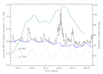
Figure 1: black line: contrast of the FOV as a function of time; blue line: contrast after rejection of structures darker than 90% of mean intensity; triangles: contrast where the apparent radius (from ephemeris) is $16.0\arcmin$

; dotted line: solar apparent radius (arc min); green line: Brussels sunspot index.

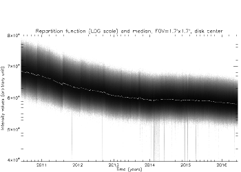
Figure 2: Time evolution of the continuum intensity histograms and median value.

The Helioseismic and Magnetic Imager (Scherrer et al., 2012; Schou et al., 2012) onboard the Solar Dynamics Observatory (SDO/HMI) provides uninterrupted full disk observations. We first extracted the continuum intensity of the 617.3 nm FeI spectral line from HMI data. We selected a FOV of $5.7\arcmin\times 5.7\arcmin$ at disk center (pixel size 0.5″) and selected data along the solar cycle from June 1, 2010 to June 20, 2016 (6 years) with a time step of 48 hours.

Figure 2 shows the monthly averaged contrast of the intensity continuum of the FOV along the solar cycle. This curve is well correlated to the Brussels sunspot index, because pores or sunspots sometimes appear close to the disk center. The contrast is defined as the ratio of the root mean square (RMS) intensity to the mean intensity over the FOV. We also show the contrast after elimination of most of the pores and sunspots: for that purpose, structures with intensity smaller than 90% (blue curve) of the mean FOV intensity were rejected. The contrast is modulated by the apparent variation of the solar radius (3% from $15.730\arcmin$ to $16.265\arcmin$); as a consequence, the pixel size varies, so that we expect an annual fluctuation of the contrast. The figure effectively reveals that the contrast (after pore or sunspot rejection) presents absolute fluctuations of approximately 0.1% or relative fluctuations 3% in phase with the apparent radius. At this stage, intensities were not filtered from photospheric 5-min oscillations, and satellite motion was not corrected either, which can slightly affect contrasts. Points where the apparent radius (from ephemeris) is $16.0\arcmin$ (every 6 months, (triangles)) show that the granulation contrast is approximately 3.5% along the solar cycle with no significant variation. The measured contrasts are reduced by a factor of 2.5 due to the instrumental PSF which is found after restoration up to $9-13\%$ (Yeo et al., 2014). Figure 2 shows the evolution in time of the intensity histograms and indicates a slowly decreasing sensitivity of the CCD. This variation does not, however, affect the contrast measurements.

2.2 Line of sight magnetic field and solar cycle

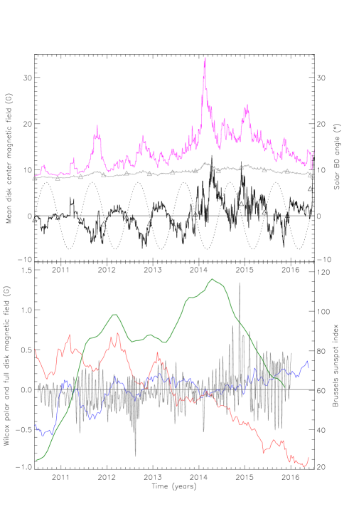
Figure 3: Top panel; black line: BLOS (Gauss) of the FOV as a function of time; violet line: mean absolute value of BLOS (Gauss) of the FOV as a function of time; gray line: same for regions with —BLOS— ¡ 100G; triangles: same, but at zero B0 angle; dotted line: disk center latitude B0 from ephemeris (degrees). Bottom panel; blue line: North pole BLOS (Gauss) from Wilcox; red line: South pole BLOS (Gauss) from Wilcox; black line: mean full disk BLOS (Gauss) from Wilcox; green line: Brussels sunspot index.

We extracted BLOS measured in FeI 617.3 nm spectral line at disk center, for the same FOV and times (June 1, 2010 to June 20, 2016, 48-hour time step), together with continuum intensities from HMI data.Here we used a reduced area of $1.7\arcmin$ x $1.7\arcmin$) in order to limit structures as pores or spots as best as possible.

Figure 3 (top) shows the monthly averaged BLOS (black) observed in the FOV along the solar cycle and Brussels sunspot index. We also show the mean BLOS magnitude (violet line) of the FOV after elimination of active regions (gray line): for that purpose, regions with $|BLOS|>100G$ were rejected. BLOS is strongly modulated by disk center latitude $B_{0}$ variations (-7.25 to 7.25 degrees). This effect is due to the annual variability of the apparent inclination of the Earth orbit with respect to the solar rotation axis. The polar magnetic field from Wilcox at North and South poles Figure 3(bottom) also exhibits the same $B_{0}$ dependance, however there is an asymmetric reversal at solar maximum, as expected, in 2013, lasting one year. Points at zero $B_{0}$ angle (every 6 months, triangles, Figure 3 (top) show that the magnetic field in the quiet network is almost constant along the solar cycle with no significant variation ( in particular regions where $|BLOS|<100G$). We therefore worked at zero $B_{0}$ in sections 4 and 5 to improve the results.

3 Observations at zero $B_{0}$ angle and data reduction

The high cadence full disk observations of SDO/HMI give a unique opportunity for mapping surface flows on various scales (both spatial and temporal). Table 1 summarizes the thirty time sequences we selected from HMI continuum intensity, Doppler and BLOS. Particular emphasis was put on only selecting dates where the magnetic field does not contain any trace of remnant activity. Such regions are supposed to represent the quietest parts of the Sun.

The selected dates have $B_{0}$ angle close to zero to avoid projection effects as emphasized by section 2. The dates run from 2010 to 2015 around June and December of each year. The $B_{0}$ angle values lie between $-1.05\degr$ and $0.61\degr$ except for the 15 and 16 October 2015 where $B_{0}$ is approximately $5.9\degr$. We used the 45 sec time series denoted $hmi.Ic\_45s$. This continuum intensity is provided by the fit to the measurements at six tuning positions of HMI during the line scan. All the time sequences were selected between 0 h and 6 h U.T.. The solar rotation has been removed along sequences in order to superimpose the data by applying a temporal shift equivalent to the equatorial rotation of 2 km/s.

The thirty 6-hour time sequences are located at disk center where we extracted a final FOV of 216.4 Mm  $\times$  216.4 Mm for all dates giving different sizes of field in pixels in the summer or winter season due to the solar radius variation. The longitudinal magnetic field and Doppler data were selected only for one hour at each date. To remove the effects of the oscillations, we applied a subsonic Fourier filter. This filter was defined by a cone in the $k$-$\omega$ space, where $k$ and $\omega$ are spatial and temporal frequencies. All Fourier components such that $\omega/k\geq V_{\rm cut-off}=6\,\mathrm{km\leavevmode\nobreak\ s}^{-1}$ were removed to keep only convective motions (Title et al., 1989). We derived horizontal velocity fields from image granulation tracking using the Local Correlation Tracking (LCT, November & Simon, 1988). Our data processing took into account the 3% variation of the pixel size on the Sun surface from 371 km in June to 360 km in December, due to the different distance between SDO and the Sun, as noticed in section 2. This correction was directly applied to the horizontal velocity amplitudes.

4 Horizontal motions derived from local correlation tracking at zero $B_{0}$

The horizontal velocity with the LCT technique were computed with a time-window of 30 min and spatial scale window of 2.5 Mm ($3.5\arcsec$). Each 6-hour sequence corresponds to twelve velocity maps. Horizontal velocities computed from the 5-min filtered solar granulation sequence have been corrected from SDO proper motions (projected velocities on the Sun of OBS_VR, OBS_VW and OBS_VN). As they are also corrected from the solar rotation and 5-min oscillations, our measurements reflect the convective flow properties.

Figure 4: Columns 1 - 4: plasma velocity of simulation for 1, 2, 5, 30 minutes and $0.13\arcsec$ time and space resolutions; column 5: plasma velocity of simulation for 30 minutes and $3.5\arcsec$ resolutions (LCT-like); column 6: LCT velocity of simulation; columns 7-8: HINODE LCT velocity for years 2007 and 2014; columns 9-10: SDO LCT velocity, averaged from 2010 to 2015, for two different FOVs of respectively $2\arcmin$ and $5\arcmin$.

It is well known that the LCT technique underestimates the real velocities due to data smoothing by a correlation window (Roudier et al., 1999; Georgobiani et al., 2007). In order to calibrate horizontal velocities obtained from the LCT algorithm, we used the results of a quiet Sun 3D MHD simulation by Stein et al. (2009). With a $0.065\arcsec$ pixel, their simulation provides the three components of the velocity field and magnetic field as a function of optical depth and time. We selected the horizontal component ($v_{x},v_{y}$) of the velocity at the solar surface at $\tau=1$ with a $0.13\arcsec$ pixel and one minute time resolution. Space and time resolutions were both degraded to the LCT windows of $3.5\arcsec$ (2.5 Mm) and 30 minutes using Gaussian smoothing. LCT horizontal velocities were computed from intensity structures (granulation) provided by the simulation. We compared this result with LCT velocities determined in the quiet Sun at disk center by HINODE (blue continuum at $0.11\arcsec$ and at $\tau=1$ and SDO continuum, at $\tau=1$, at $0.50\arcsec$ pixel size, as described above. The three data sets are all observed and simulated at the intensity continuum at $\tau=1$ corresponding to the same height of formation. Figure 4 shows the comparison between plasma velocities derived from the simulation at the LCT resolution and LCT velocities issued from structure tracking, for the simulation as well as HINODE and SDO. We found that LCT results are consistently underestimated by a factor 0.52, 0.61 and 0.38 for the simulation, HINODE and SDO, respectively, so that in the following, the SDO LCT horizontal velocities were multiplied by the a factor of 2.63.

Figure 5 shows that during the cycle the mean velocity magnitude over the 6-hour sequence is $0.645\pm 0.010$ km/s while the median value (not displayed) lies at $0.595\pm 0.010$ km/s. No significant variation is observed during the period 2010 to 2015 although maximum solar activity is reached in 2014. We also found that the root mean square (RMS) of the horizontal velocity remains stable at approximately $0.355\pm 0.010$ km/s during the solar cycle. This stability is confirmed by velocity histograms over the cycle that exhibit quite similar shapes with very little dispersion (Figure 6). The contrast does not reveal any variation in time, corroborating preliminary conclusions of section 2 and previous results found by Muller et al. (2007).(private communication).

Figure 5: Mean magnitude (plus signs) and RMS (crosses) of horizontal velocities from 2010 to 2015.

Figure 6: Histograms of horizontal velocities of the thirty sequences from 2010 to 2015.

4.1 Divergence and vorticity properties

Figure 7: Evolution of mean divergence (plus signs) and vorticity (crosses) magnitudes of horizontal velocities from 2010 to 2015.

As the measured velocity field is purely two-dimensional, two quantities are relevant to characterize flow structures: the divergence $D=\partial_{x}v_{x}+\partial_{y}v_{y}$ and the $z$-component of the vorticity $\zeta=\partial_{x}v_{y}-\partial_{y}v_{x}$.

Figure 7 reveals that both divergence and rotational magnitudes do not present any significant variation, indicating again that flow properties remain similar over the FOV during the solar cycle. The mean values are $3.68\leavevmode\nobreak\ 10^{-4}\leavevmode\nobreak\ s^{-1}$ for the divergence and $3.38\leavevmode\nobreak\ 10^{-4}\leavevmode\nobreak\ s^{-1}$ for the vorticity. We notice a small increase in vorticity between 2010 and 2015, which does not correlate with solar activity.

4.2 Diffusion index

Figure 8: Evolution of the diffusion index from 2010 to 2015. Mean values for each date are represented by diamonds.

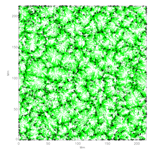
Figure 9: Trajectories of corks (green lines) and their final locations (black crosses) after 6-hour evolution. The ending positions delineate the network.

The transport of the magnetic element on the photosphere is well described by a power law $<(\Delta r)^{2}>=c\leavevmode\nobreak\ t^{\gamma}$ where $<(\Delta r)^{2}>$ is the mean square displacement, $c$ a constant, $t$ the time measured since the first detection, and $\gamma$ the spectral index (Giannattasio et al., 2014). Following passive scalars, such as corks over a long time scale, allows for measurement of this reference index. Figure 8 shows that the mean index (diamond) lies in the range 1.32$-$1.36 but we do not detect any variation correlated with the cycle, indicating that quasi-stable flows occur at the Sun surface and drive magnetic elements to form the quiet network (Figure 9).

4.3 Cell properties along the cycle

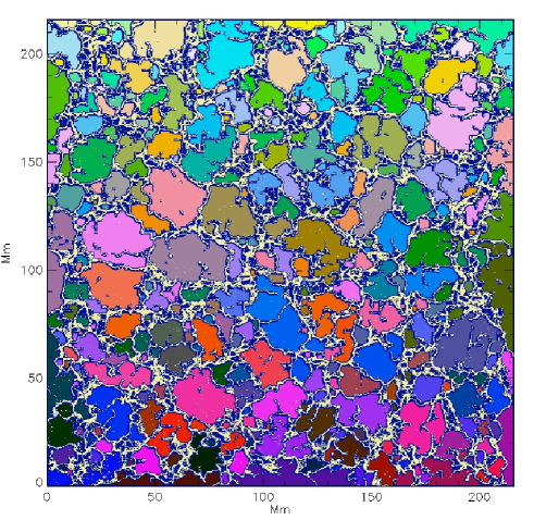
Figure 10: Network location (yellow for cork final positions) surrounding the detected cells shown in various colors.

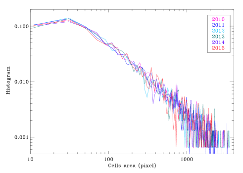
Figure 11: Cell area histograms from 2010 to 2015.

The cork trajectories due to horizontal velocities have been computed over 6 hours for each sequence. We observe that the corks are expelled from diverging cells with size from meso- to supergranular scales as expected. The corks locations at the end of the sequence (Figure 10) delineate a network from which we extracted cells by a segmentation process (Roudier et al., 1999). As the temporal sequence is relatively short (6 hours), smaller cell sizes are privileged but the same treatment is applied to all sequences allowing a quantitative comparison. Figure 11 exhibits the mean cell area histograms (i.e., the fraction of the number of cells for each area bin) for each year. We observe a monotonic decrease towards the larger scales but the different histograms are similar, confirming that the size of cells formed by horizontal flows does not vary significantly over the solar cycle in the quiet Sun.

5 Magnetic field, intensity contrast and Doppler properties during the cycle at zero $B_{0}$

5.1 Magnetic field and intensity contrast temporal evolution

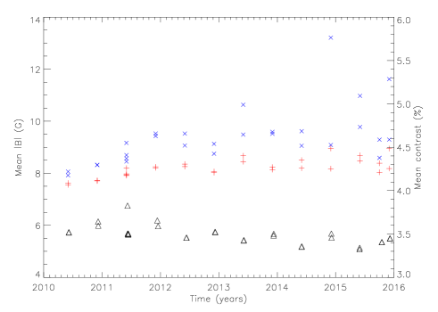
Figure 12: Time evolution of the magnitude of BLOS (blue crosses), magnetic field in regions where $|BLOS|<100G$ (red crosses) and intensity contrasts (black triangles).

Figure 13: Time evolution of the intensity contrasts (triangles) and of fluctuations of the velocity module of the SDO satellite (crosses).

Observations over the entire disk of the longitudinal magnetic field and Doppler velocities are provided by SDO/HMI.

Figure 12 shows no particular variation trend of the magnitude of the magnetic field during the cycle (which corroborates results of Figure 3 at varying $B_{0}$). The larger value of $|BLOS|$ on December 4, 2014, is due to a small residual active region in the upper right corner of the field. Figure 12 also displays the magnitude of magnetic fields in regions where $|BLOS|<100G$. We observe a better stability in very quiet regions of the Sun.

Continuum intensity contrasts of Figure 12 are derived from the average of the contrast of each image in the 6-hour sequence. Contrast was corrected from pixel size fluctuations (3%) due mainly to the varying apparent radius. However, the continuum intensity is one of the outputs of a fit to the measurements at the six tuning positions of HMI during the line scan. When orbital or solar velocities are large this can introduce artifacts in the continuum intensity. As shown in Figure 13, the constrast intensity is well correlated with velocity fluctuations of the SDO satellite. The intensity contrast is clearly modulated by SDO proper motions giving a lower variation than those plotted in figure  12. In conclusion, the intensity contrast does not reveal any variation in time, corroborating preliminary conclusions of section 2 and previous results found by Muller et al. (2007) and Muller (private communication).

5.2 Doppler temporal evolution

Figure 14: Plus signs: mean value of VLOS magnitude (km/s); triangles: RMS VLOS (km/s).

The Doppler velocity was obtained at disk center for 1 hour over a 216.4 Mm  $\times$  216.4 Mm. FOV (Table 1) at zero $B_{0}$, in order to avoid the annual modulation described above for BLOS (section 2). The HMI Doppler signal is formed at a height of approximately 100 km ((Fleck et al., 2011)).

The line of sight Doppler velocity VLOS was first corrected from 5 min oscillations in the $k$ and $\omega$ diagram using the classical filter $\omega<V_{\rm cut-off}\times k$ where $V_{\rm cut-off}=6\,\mathrm{km\leavevmode\nobreak\ s}^{-1}$ in order to isolate the convective component.

VLOS was then corrected in latitude and longitude from the solar rotation using a differential rotation law of the form (in degrees per day) :

$$\Omega=14.41-2.83*\sin^{2}\theta$$ (1)

The latitude $\theta$, proportional to y, allows computation of the angular velocity as a function of y. Hence, the projection of the rotation speed on the LOS is a function of x and y which was subtracted from VLOS. Thus VLOS has a zero average value over the FOV.

Figure 14 shows that we do not detect any VLOS variation along the solar cycle.

6 Discussion and conclusions

The solar cycle was originally found through the variations in the number of sunspots, which are easily observable. Besides, we know that the quiet Sun is far from devoid of magnetic field. Changes in the dynamics of the quiet Sun could have a large effect on its overall properties, such as the photospheric temperature or magnetic field generation (flux tubes). In many cases, the existence of variations with the solar cycle of various quiet Sun parameters, has yet to be demonstrated. Understanding the mechanism that diffuses magnetic fields over the solar surface is still an important challenge, because the network contribution to the global solar magnetism is known to be comparable to the flux of active regions at maximum activity. As the global magnetic field of the Sun has an activity cycle, one expects to observe some variations in the dynamical properties of the flows in the photosphere. The comparison with different phases of the solar cycle studied by Palle et al. (1995) reveals a high stability of the solar granulation while mesogranulation is dependent. As some variations of the supergranulation (Rimmele & Schroeter, 1989) and granulation (Muller, private communication) are observed with latitude, our measurements at disk center reveal the stability of the flow properties between meso- and supergranular scales along the solar cycle. In our study, we took care to select very quiet regions without any residual activity. In such regions, the detected magnetic field is probably generated by the local dynamo process to form the quiet network. Utz et al. (2016) describe a link between the magnetic bright point (MBP) activity close to the equator and the global magnetic cycle. They indicate that a significant fraction of MBPs originate from the sunspot activity belt. Thus the magnetic network behavior appears to be related to solar activity but its variation is essentially fed by the decay of active regions (Thibault et al., 2014). Our analysis seems to indicate that the magnetic field produced locally at disk center (Gošić et al., 2014), independently from the large scale dynamo, forms what we call the very quiet Sun, and remains unchanged along the solar cycle. Thus the irradiance contribution of the very quiet network is also likely be constant in time. The latitudinal variation of the network properties (Ishikawa et al., 2010) and related irradiance, could be essentially due to the magnetic field coming from active regions dispersed by differential rotation, meridian and supergranular flows (van Driel-Gesztelyi & Green, 2015).

The present work has been concentrated on large scales as meso$-$ and super$-$ granulation; further analysis will be extended to the solar granulation dynamics along the cycle. Indeed, the observed parameters of the quiet Sun (intensity, velocity, and field strength) are constrained by the spatial resolution of HMI. This does not a priori exclude that changes could be occurring at smaller spatial scales than meso- and supergranulation.