The fourth dimension of the nucleon structure: spacetime analysis of the timelike electromagnetic proton form factors

Abstract

As well known, spacelike proton form factors expressed in the Breit frame may be interpreted as the Fourier transform of static space distributions of electric charge and current. In particular, the electric form factor is simply the Fourier transform of the charge distribution $F(q)=\int e^{i\vec{q}\cdot\vec{r}}\rho(r)d^{3}r$. We don’t have an intuitive interpretation of the same level of simplicity for the proton timelike form factor appearing in the reactions $e^{+}e^{-}\leftrightarrow\bar{p}p$. However, one may suggest that in the center of mass (CM) frame, where $q_{\mu}x^{\mu}=qt$, a timelike electric form factor is the Fourier transform $F(q)=\int e^{iqt}R(t)dt$ of a function $R(t)$ expressing how the electric properties of the forming (or annihilating) proton-antiproton pair evolve in time. Here we analyze in depth this idea, show that the functions $\rho(r)$ and $R(t)$ can be formally written as the time and space integrals of a unique correlation function depending on both time and space coordinates.

I Introduction

I.1 Background

The reaction $e^{+}+e^{-}\to\bar{p}+p$ and its time reverse $\bar{p}+p\to e^{+}+e^{-}$ have been used to extract the electromagnetic form factors (FFs) of the proton in the time-like (TL) region. Assuming that the interaction occurs through one photon exchange, the annihilation cross section is expressed in terms of the FF moduli squared (Zichichi et al. (1962), see also Pacetti et al. (2015); Denig and Salme (2013) for recent reviews on TLFF).

The empirical knowledge and the theoretical understanding of the TLFF are less advanced than for the spacelike (SL) case. In particular, an experimental separation of the electric and the magnetic FF has not been possible in the TL region, because of the available limited luminosity. The cross section $\sigma$ of the above reactions allows to extract the squared modulus of a single effective form factor $F_{p}$ Bardin et al. (1994)

$$|F_{p}|^{2}=\displaystyle\frac{3\beta q^{2}\sigma}{2\pi\alpha^{2}\left(2+\displaystyle\frac{1}{\tau}\right)},$$ (1)

where $\alpha=e^{2}/(4\pi)$, $\beta=\sqrt{1-1/\tau}$, $~{}\tau={q^{2}}/(4M^{2})$, $q^{2}$ is the squared invariant mass of the colliding pair, and $M$ is the proton mass. The effect of the Coulomb singularity of the cross section at the $\bar{p}p$ threshold is removed by the $\beta$ factor: $\beta$ $\rightarrow$ 0 for $q$ $\rightarrow$ $2M$, so that $\beta\sigma$ is finite and the effective form factor is expected to be finite at the threshold.

This effective TLFF has been measured by several experiments for $q^{2}$ ranging from the threshold $(2M_{N})^{2}$ to about 36 GeV². The most recent and precise results from the BABAR Lees et al. (2013a, b) and BESIII collaborations Ablikim et al. (2015) are reported in Fig. 1.

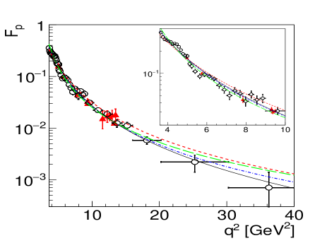
Fig. 1: Most recent data on the TL proton generalized FF as a function of $q^{2}$, from Refs. Lees et al. (2013a, b) (black open circles), Refs. Ablikim et al. (2005) (red triangles), together with the calculation from Eq. (2) (blue dash-dotted line), Eq. (3) (red dashed line), Eq. (4) (green long-dashed line), and Eq. (5) (black solid line).

These data have been fitted by some parameterizations. Here we report four of them, to give an idea of the general trend followed by the data and of the related ambiguities in extrapolations to the large $q$ region. Details about these fits and the best fit parameters can be found in our previous works Bianconi and Tomasi-Gustafsson (2015, 2016). In the experimental papers before the year 2006, the function Ambrogiani et al. (1999); Lepage and Brodsky (1979):

$$|F_{scaling}(q^{2})|=\displaystyle\frac{\cal A}{(q^{2})^{2}\log^{2}(q^{2}/\Lambda^{2})},\ {\cal A}=40~{}\mbox{GeV}^{-4},\ \Lambda=0.45~{}\mbox{GeV}^{2}.$$ (2)

was frequently used. The modification

$$|F_{scaling+corr}(q^{2})|\ =\ \displaystyle\frac{\cal A}{(q^{2})^{2}\left[\log^{2}(q^{2}/\Lambda^{2})+\pi^{2}\right]},\ {\cal A}=72~{}\mbox{GeV}^{-4},\ \Lambda=0.52~{}\mbox{GeV}^{2}.$$ (3)

was suggested Shirkov and Solovtsov (1997); Kuraev (2008) to avoid problems with ghost poles in $\alpha_{s}$. In Ref. Brodsky and de Teramond (2008) a pure rational form was proposed, with two poles of dynamical origin

$$|F_{T3}(q^{2})|\ =\ \displaystyle\frac{\cal A}{(1-q^{2}/m_{1}^{2})(2-q^{2}/m_{2}^{2})},\ {\cal A}=1.56,\ m_{1}^{2}=1.5,\ \mbox{GeV}^{2},\ m_{2}^{2}=0.77\ \mbox{GeV}^{2}.$$ (4)

The TLFF data from the BABAR collaboration Lees et al. (2013a, b) extending from the threshold to $q^{2}$ $\approx$ 36 GeV², are steeper than the previous data, and are well reproduced by the following rational fit Tomasi-Gustafsson and Rekalo (2001):

$$|F_{BABAR}(q^{2})|\ =\ \frac{\cal A}{(1+q^{2}/m_{a}^{2})\left[1-q^{2}/0.71\right]^{2}},~{}{\cal A}=7.7~{}\mbox{GeV}^{-4},~{}\ m_{a}^{2}=14.8~{}\mbox{GeV}^{2}.$$ (5)

where a $q^{4}$ asymptotic trend is not visible, although the data points at $q>$ 4 GeV present too large error bars to constrain the large-$q$ trend of a fit. For $q<$4 GeV the data also show oscillating 10 % modulations around the previous fits. In our works Bianconi and Tomasi-Gustafsson (2015, 2016), we have fitted the BABAR data with

$$F(p)\ \equiv\ F_{0}(p)\ +\ F_{osc}(p),$$ (6)

where $p=p(q)$ is the relative three-momentum of the final hadron pair, $F_{0}(p)$ is any of the previous fits. Eqs. (2-5) are expressed in terms of $p(q)$, and the modulation term $F_{osc}(p)$ is parameterized as

$$F_{osc}(p)\ \equiv\ A\ e^{-Bp}\ \cos(Cp\ +\ D).$$ (7)

The precise values of the parameters depend on which of the previous four fits is chosen as leading term $F_{0}$. A list of best fit values for all these cases is presented in Bianconi and Tomasi-Gustafsson (2016). In all cases $D\approx$0 and $A$ has magnitude $\simeq 0.1$. This means that the first oscillation is also a threshold enhancement, like those found in $e^{+}e^{-}\rightarrow\bar{n}n$, $e^{+}e^{-}\rightarrow\bar{\Lambda}\Lambda$ and other production processes of neutral baryon pairs Ablikim et al. (2010); Pakhlova et al. (2008); Ablikim et al. (2006, 2004); Bai et al. (2003); Amsler et al. (1994).

These near-threshold phenomena should disappear at large $q^{2}$, so that the data and their fits may converge to the simple quark counting rule: TLFF $\propto$ $1/q^{4}$, as predicted for the SLFF asymptotic Matveev et al. (1973); Brodsky and Farrar (1973).

This may be stated by using the same arguments of the SL case, that is by analyzing the dimensional structure of the matrix element Matveev et al. (1973) or by assuming that at large $q$ the process is dominated by a PQCD hard core Brodsky and Farrar (1973), or by using analytic continuation at large $|q|$ from the SL to the TL sector (applying the Phragmèn-Lindelöf theorem, see the discussion in Tomasi-Gustafsson and Rekalo (2001)). In all cases, the details of the soft part of the $\bar{p}p$ creation or annihilation process do not play a role. On the other hand, these features are expected to heavily affect the finite-$q$ deviations from the $1/q^{4}$ rule, and to determine the FF magnitude and phase. This has prompted several studies of the nonperturbative aspects of the TLFF. Some effects of bound-state gross features on PQCD calculations, leading to pre-asymptotic differences between TLFF and SLFF, were studied in Ref. Gousset and Pire (1995), still within a largely perturbative scheme.

Several detailed nonperturbative models for the nucleon or meson TLFF have been proposed: some derive from a unique analytic prediction valid both in the SL and in the TL region, other ones are more specific. There are approaches based on vector meson dominance Bijker and Iachello (2004); Adamuscin et al. (2005) and dispersion relations Belushkin et al. (2007); Lomon and Pacetti (2012). They give precise quantitative predictions for a large set of observables and have been applied Bianconi et al. (2006a, b), to simulate the feasibility of high-precision experiments including polarization observables and two-photon contributions Gakh and Tomasi-Gustafsson (2005, 2006).

In de Melo et al. (2004) a mixed approach to the pion TLFF is present, where VDM is applied at the level of photon-quark-antiquark vertex, but also a constituent quark loop and quark-pion couplings are present. In addition, a large number of poles is used, with parameters partly determined by phenomenology and partly by a dynamic model. Later on, non valence 4-constituent states have been added de Melo et al. (2006). The approach based on AdS/QCD correspondence used in Ref. Brodsky and de Teramond (2008), may be considered a pole-based model (see previous Eq. (4)), although in this case the poles are not a starting assumption but rather the arrival point of a complex procedure.

A distinguishing feature of the model presented in Kuraev et al. (2012) is that it is built in spacetime, instead of momentum space. A large-$q$ suppression of the ratio of the electric to the magnetic FF in both the SL and TL sectors is suggested by a qualitative picture, where, in an intermediate stage of the hadron formation process, the reaction region is divided into a central region that is neutral from the color and flavor points of view, and a peripheral region where these properties are localized. At increasing $q$ this suppresses the overlap between the electric charge of the proton-antiproton pair, and the $1/q$-sized virtual photon. The suppression does not necessarily apply to the magnetic FF since a magnetic moment is not localized on the physical currents producing it.

These models were targeted at the leading features of the data shown in Fig. 1, the “regular” behavior reproduced by the above fits (2-5). The oscillations of Eqs. (6-7), appearing as a periodic modulation, were interpreted in Refs. Bianconi and Tomasi-Gustafsson (2015, 2016) as an interference phenomenon in spacetime, with competition between processes involving well separated regions with different properties. In particular, regions closer to the $\gamma^{*}-q\bar{q}$ vertex would present regeneration properties for the $\bar{p}p$ wave function, while suppression of this state would occur in more peripheral regions. Starting from a different point of view, another fit to the oscillations of the TLFF was proposed by Lorenz et al. (2015) as a sum of independent structures like resonance poles and intermediate state thresholds. Interference in spacetime and poles in $q$ could be alternative ways to describe a similar mechanism: for the case of the pion TLFF, several oscillations regularly spaced in $q^{2}$ are predicted in the model by de Melo et al. (2004). Although they are due to the contribution of of many resonance states, these oscillations present a regularity pattern because of a unique dynamic model behind these resonances.

The interpretation of the threshold enhancement is related to the oscillation problem, since the threshold enhancement can be seen as the first oscillation, although it seems especially evident in the TLFF of neutral baryons. The authors of Ref. Haidenbauer et al. (2014) suggest that it is due to proton-antiproton strong interactions in low energy conditions. A different explanation was suggested by Baldini et al. (2009), in terms of local electric interactions between quarks and antiquarks of the two baryons. This is equivalent to a reciprocally induced electric polarization of the interacting spin-1/2 hadrons. Although nonstandard, the same mechanism has been used to explain the near-threshold rise of the inelastic antineutron cross sections in Bianconi et al. (2014), and may find a justification in the calculation of a neutron electric polarization induced by a strong external electric field due to QED vacuum polarization terms Zimmer et al. (2012).

I.2 Aim of the present work

Summarizing the previous discussion, the attempts to reproduce the non-perturbative aspects of TLFF data introduce complex and largely unexplored details of the hadron-pair formation process. Translating a model for TLFF into a spacetime picture of the hadron pair formation process is not immediate, however, since relativistic amplitudes are normally handled in momentum space, and the processes involving pair creation or annihilation do not have an intuitive nonrelativistic equivalent. The starting question of the present work is how one can translate data fits or models of TLFF into intuitive spacetime pictures of the forming or annihilating proton-antiproton system, similarly to what happened for SLFF.

In the SL case, FFs in the Breit frame ($q_{0}=$ 0, no energy transfer) may be interpreted in a standard nonrelativistic way, as Fourier space transforms of stationary charge and current distributions. The interpretation of the SLFF in terms of charge-current distribution has transformed a mathematical abstraction, that only experts of field theory may understand, into something that has a tangible meaning for a much broader audience.

The SLFF interpretation in terms of a charge density cannot be extended to the TL case, since the photon time-like momentum can test time distributions of events, but not space distributions. In the CM frame of the $e^{+}e^{-}$ collision the photon has zero three-momentum (infinite space wavelength) so any effect related to space separation of electric charges is not detectable by it. Whatever is tested by the virtual photon, it must be a function $R(t)$ of the time deriving from an average over all the three-space. But, after a three-space average, the overall electric charge of the forming hadron-antihadron pair is equal to zero at any time. Of course, this concerns the ”electric charge” in the classical electrodynamical sense, that is the source of an electromagnetic field. If we interpret the concept of ”charge” as ”photon-charge coupling”, we may think at $R(t)$ as an amplitude for creating charge-anticharge pairs at the time $t$. So, ‘”charge distribution” can be understood as ”distribution in time of $\gamma^{*}\rightarrow charge-anticharge$ vertexes”.

In the following, we will examine in depth this idea, formalize the relation between $R(t)$ and the static space charge density $\rho(r)$ that is measured in the SLFF, and present some examples inspired by the phenomenology.

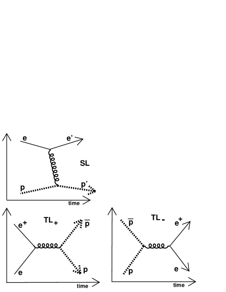
Fig. 2: Feynman diagrams for reactions (8): labeled as SL in the figure, (9): TL₊, and (10): TL_-. In the one photon exchange approximation, electromagnetic FFs are functions characterizing the vertex coupling the virtual photon to the hadron current (thick dashed line in the figure).

II General definitions

The relevant reactions for the extraction of SL and TL FFs are:

$$SL:\ e^{\pm}+p\to e^{\pm}+p,$$ (8)

$$TL_{+}:\ e^{+}+e^{-}\to\bar{p}+p,$$ (9)

$$TL_{-}:\ \bar{p}+p\to e^{+}+e^{-}.$$ (10)

They are related by crossing symmetry and illustrated in Fig. 2. Reaction (8) allows for measuring the FF in the spacelike (SL) kinematical region, corresponding to a virtual photon four-momentum $q_{\mu}$ with ${\vec{q}}^{2}>q_{0}^{2}$. Reactions (9) and (10), allow for exploring the timelike (TL) FFs, more precisely, the processes (9) and (10) are labeled $TL_{+}$ and $TL_{-}$ respectively.

We assume one-photon exchange, so in the following ”form factor” is meant as a factor renormalizing the hadron-virtual photon vertex, as in Fig. 3. Factorizing out the lepton part of the process and the virtual photon propagation, we will only consider the three-leg amplitude $A(q,P_{A},P_{B})$ describing the sub-processes of the reactions introduced above:

$$SL : \ \gamma^{*}(q_{\mu})\ +\ p(p_{\mu})\rightarrow p(p_{\mu}^{\prime})$$ (11)

$$TL_{+} : \ \gamma^{*}(q_{\mu})\ \rightarrow p(p_{\mu}^{\prime})\ +\ \bar{p}(\bar{p_{\mu}}^{\prime})$$ (12)

$$TL_{-} : \ p(p_{\mu})\ +\ \bar{p}(\bar{p}_{\mu})\ \rightarrow\gamma^{*}(q_{\mu}^{\prime})$$ (13)

The four-momenta $q^{\mu}$, $P_{A}^{\mu}$, $P_{B}^{\mu}$ appearing as $formal$ arguments of $A(q,P_{A},P_{B})$ are all incoming as in Fig. 3, so that the different reactions are distinguished by the expression of $q$, $P_{A}$ and $P_{B}$ in terms of the $physical$ momenta $q$, $q^{\prime}$, $p$, $p^{\prime}$, $\bar{p}$, $\bar{p}^{\prime}$ (that have a positive time component if they are timelike):

$$\gamma^{*}+p\rightarrow p^{\prime}\hskip 25.6073pt(SL:\ |q_{0}|\ <\ |\vec{q}|)\ \hskip 51.21504pt P_{A}\ =\ p,\ P_{B}\ =\ -p^{\prime},$$ (14)

$$\gamma^{*}\rightarrow\bar{p}+p\hskip 28.45274pt(TL_{+}:\ |q_{0}|\ >\ |\vec{q}|,\ q_{0}\ >\ 0)\ P_{A}\ =\ -p^{\prime},\ P_{B}\ =\ -\bar{p}^{\prime}.$$ (15)

$$\bar{p}+p\rightarrow\gamma^{*}\hskip 28.45274pt(TL_{-}:\ |q_{0}|\ >\ |\vec{q}|,\ q_{0}\ <\ 0)\ P_{A}\ =\ p,\ P_{B}\ =\ \bar{p},\ q\ =\ -q^{\prime}.$$ (16)

whereas, in the TL region, two reciprocally inverse reactions are possible, corresponding to $\bar{p}p$ annihilation into (or creation from) a lepton-antilepton pair.

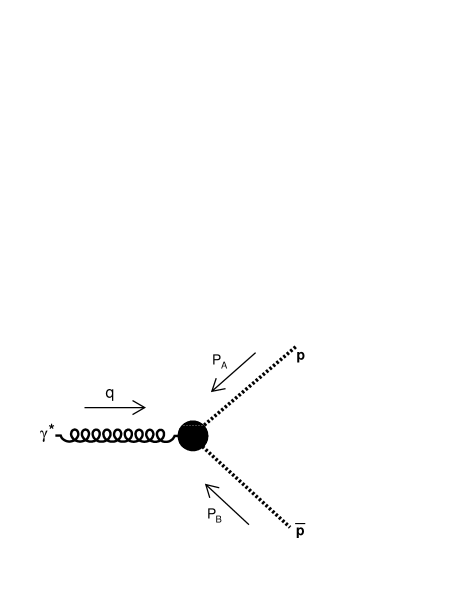
Fig. 3: Subdiagram participating to the three reactions (14-16). Since they may be considered physical channels of the same reaction, all of them may be described by the same diagram and by the same amplitude by changing the values of the components of the four-momenta $P_{A}$, $P_{B}$, $q$, exploiting crossing symmetry. Formally, we consider these momenta as all entering. So, $q$ coincides with the physical four-momentum of the virtual photon in the channel $TL_{+}$ where a $\bar{p}p$ pair is created, while $q=-q^{\prime}$, where $q^{\prime}$ is the physical four-momentum of the virtual photon, in the reverse channel $TL_{-}$ where a virtual photon is produced by $\bar{p}p$ annihilation. Similar considerations apply to $P_{A}$ and $P_{B}$ (see Eqs. (14-16) for the correspondence between the formal arguments of the amplitude and the physical momenta).

It is important not to confuse the four-momenta $P_{A},P_{B}$, as formal arguments of $A$, with their physical values $\pm p$, $\pm\bar{p}$ etc: the analytic continuation of $A(q,P_{A},P_{B})$ requires that this amplitude is described in terms of the same arguments in all the reaction channels and in the unphysical regions (so, $q_{0}<$ 0 in one of the two annihilation channels, and it is, in general, a complex variable). Being $A(q,P_{A},P_{B})$ invariant, it actually depends on $q$, $P_{A}$ and $P_{B}$ via their invariant products only, so these three four-vectors contain redundant information. However, in the following, we keep the formal dependence of $A$ on them.

Here we distinguish between ”resolvable” and ”unresolvable” particles. A resolvable particle participates to a process with its internal structure, while an unresolvable particle is treated as a massive elementary particle. Both levels are present in the FF analysis. As an unresolvable particle, the photon-hadron current interaction takes place in a single vertex four-point $X_{\mu}$. The FF takes into account that at a resolvable level the photon-hadron interaction involves several variables $X_{1}^{\mu},X_{2}^{\mu},...$ associated to the internal hadron constituents. From now on we omit the tensor indexes and just write $X$, $X_{1}$ etc.

Assuming a muon as a template for an unresolvable proton, the vertex matrix element for $\gamma(q)+\mu(p)\rightarrow\mu(p^{\prime})$ is (using $\bar{u}\gamma^{0}=u^{+}$)

$$A_{point\ SL}(q,p,p^{\prime})\ =\ <\mu^{\prime}|A_{\nu}(X)J^{\nu}(X)\ |\mu>\ =\ e\int d^{4}X\ e^{iqX}\ e^{-ip^{\prime}X}\ e^{ipX}\ e_{\nu}\ \bar{u}(p^{\prime})\gamma^{\nu}u(p)\ =\$$ (17)

$$=\ e\int d^{4}Xe^{iqX}e^{-ip^{\prime}X}e^{ipX}\Big{(}e_{0}\ u^{+}(p^{\prime})u(p)\ -\ \vec{e}\ \bar{u}(p^{\prime})\vec{\gamma}u(p)\Big{)}\ =$$ (18)

$$=\ \delta^{4}(q+p-p^{\prime})\ \Big{(}T_{point\ charge}(q,p,p^{\prime})\ -\ T_{point\ current}(q,p,p^{\prime})\Big{)}.$$ (19)

Exploiting that the amplitudes of the processes (15) and (16) are analytic continuations of the amplitude of (14), we can write Eq. (19) in a form where it describes all these processes:

$$A_{point}(q,P_{A},P_{B})\ \equiv\ \delta^{4}(q+P_{A}+P_{B})\ \Big{(}T_{point\ charge}(q,P_{A},P_{B})\ -\ T_{point\ current}(q,P_{A},P_{B})\Big{)},$$ (20)

where, assigning to $q$, $P_{A}$, $P_{B}$ the values listed in Eqs. (14-16), we obtain the amplitudes for the corresponding reactions.

FFs may be introduced as scalar functions that multiply the previous terms, or linear combinations of these terms:

$$A(q,P_{A},P_{B})\ \equiv \ A_{charge}(q,P_{A},P_{B})\ -\ A_{current}(q,P_{A},P_{B})$$ (21)

$$\equiv\ \delta^{4}(q+P_{A}+P_{B})\ \bigg{(}T_{point\ charge}(q,P_{A},P_{B})\ F(q)\ -\ T_{point\ current}(q,P_{A},P_{B})\ G(q)\bigg{)},$$ (22)

where now this amplitude describes processes involving proton and antiproton instead of muons. The scalar FFs $F(q)$ and $G(q)$ depend on $q_{\mu}$ via the scalar $q^{2}$ $\equiv$ $q_{\mu}q^{\mu}$ only. Alternatively, one may rewrite the hadron four-current in the Gordon form, insert $F_{1}$ and $F_{2}$ and next combine them into $G_{E}$ and $G_{M}$. However, the adopted procedure is simpler, since it immediately highlights the term that is proportional to the charge density operator $u^{+}(p^{\prime})u(p)$. We will not work on the other component in the following. In the relevant reference frames (the Breit frame for the SL case and the CMS for the TL case) $F(q)$ coincides with the electric form factor $G_{E}$. In an arbitrary frame, $F(q)$ is a linear combination of $G_{E}$ and $G_{M}$.

Our further analysis only considers the form factor $F(q)$ associated with the charge term. So our starting equation is:

$$A_{charge}(q,P_{A},P_{B})\equiv\ \delta^{4}(q+P_{A}+P_{B})\ T_{point\ charge}(q,P_{A},P_{B})\ F(q)$$ (23)

III Fourier transform of the FF. SL-Breit and TL-CM cases, time density of photon-quark coupling.

Following a suggestion from Kuraev et al. (2012), the key tool of our investigation is the four-dimensional Fourier transform

$$F(q)\ =\ \int d^{4}xe^{iqx}F(x).$$ (24)

In the SL case, and in the Breit frame where $q^{\mu}=(0,\vec{q})$,

$$F_{SL,Breit}(q)\ =\ \int d^{3}\vec{x}\ e^{-i\vec{q}\cdot\vec{x}}\int dtF(t,\vec{x})\ \equiv\ \int d^{3}\vec{x}\ e^{-i\vec{q}\cdot\vec{x}}\rho(|\vec{x}|)$$ (25)

$$\rho(|\vec{x}|)\ =\ \int dtF(t,\vec{x}).$$ (26)

where $\rho(|\vec{x}|)$ may be read as a static charge density. Here it appears as a time average over the Fourier transform $F(x)=F(t,\vec{x})$.

In the TL case, and in the CM frame ($\vec{q}$=0)

$$F_{TL,CM}(q)\ =\ \int dt\ e^{iqt}\int d^{3}\vec{x}F(t,\vec{x})\ \equiv\ \int dt\ e^{iqt}R(t),$$ (27)

$$R(t)\ =\ \int d^{3}\vec{x}F(t,\vec{x}).$$ (28)

It is evident that it is difficult, in absence of a model for the underlying $F(x)$ (that depends on both $\vec{x}$ and $t$), to find a simple relation between $\rho(\vec{x})$ and $R(t)$, since they represent projections of the same distribution onto orthogonal subspaces.

IV General properties of F(x)

Since we have required $F(q)$ to depend on the four-vector $q_{\mu}$ via $q^{2}$ only, $F(x)$ is constrained to have the form:

$${\vec{x}}^{2}\ >\ t^{2}:\ F_{outLC}(x_{\mu})\ =\ f(x^{\mu}x_{\mu}).$$ (29)

$$t^{2}\ >\ {\vec{x}}^{2}:\ F_{inLC}(x_{\mu})\ =\ f_{+}(x^{\mu}x_{\mu})\theta(t)\ +\ f_{-}(x^{\mu}x_{\mu})\theta(-t)$$ (30)

where we distinguish the “in light-cone” and the “out of light cone” components of $F(x)$. For $F_{outLC}(x_{\mu})$, a $t\to-t$ asymmetry is forbidden by the requirement that symmetry properties of a scalar amplitude do not depend on the reference frame (a positive $t$ can be made negative by a proper Lorentz boost). Since a proper Lorentz boost cannot mix future and past light cones, the same constraint is not present on $F_{inLC}(x_{\mu})$, that may be rewritten as

$$F_{inLC}(x_{\mu})\ =\ 1/2\ [f_{+}+f_{-}]\ +\ 1/2\ [f_{+}-f_{-}][\theta(t)-\theta(-t)]$$ (31)

The last term is important since it leads to an imaginary part of $F(q)$ even if $F(x)$ is real.

The $f_{+}-f_{-}$ term implies asymmetries between the reactions $\gamma^{*}$ $\rightarrow$ $\bar{p}$ $+$ $p$ and $\bar{p}$ $+$ $p$ $\rightarrow$ $\gamma^{*}$, supposedly associated with final/initial state interactions. These asymmetries are constrained by the T-reversal requirement that $|F(q)|$ is not changed by $q_{0}$ $\rightarrow$ $-q_{0}$ (proton-antiproton annihilation instead of creation), so the differences affect only phases.

In absence of a physical model, there is no mathematical reason to prevent the TL form factor $F(q)$ from receiving contributions from the SL regions of $x_{\mu}$ and viceversa for the SL form factor. A simple example may confirm this: in the $(1+1)$-spacetime $(t,z)$ we may take $F(t,z)$ $=$ $\delta(z^{2}-t^{2}-1)$, that is zero in the TL region $z^{2}$ $\leq$ $t^{2}$ including its borders. In the CM frame $R(t)$ $\equiv$ $\int dzF(t,z)$ $=$ $(1+t^{2})^{-1/2}$. For real $t$, $R(t)$ admits a nonzero, real and regular (although analytically nontrivial) Fourier transform $F(q)$.

On the contrary, within a physical model where relativistic causality is implemented, the TL domains of $x$ are related to the TL domains of $q$. To demonstrate this, we need to discuss some of the physical content of $F(x)$. Up to now, $F(x)$ has just been introduced as the Fourier transform of a form factor. We now rewrite Eq. (23), assuming a model where the virtual photon conversion into a proton-antiproton pair begins with the photon conversion into a quark-antiquark pair, and all the other steps of the process follow causally from this initial event.

The amplitude describing how a free (anti)proton with momentum $p$ splits into a Fock state of $N$ constituents is

$$\psi(X_{1},X_{2},....X_{N})\ \equiv\ e^{ipX}\Phi(x_{1},x_{2},...x_{N})$$ (32)

where the four-factor $X_{i}$ is the spacetime position of the i-th constituent, $X$ is a linear combination of all the $X_{i}$, expressing the spacetime position of the proton as a whole (the unresolved proton) and the four-coordinates $x_{i}$ are internal four-coordinates relative to $X$:

$$X\ =\ \sum w_{i}X_{i},\ i=1,....N.$$ (33)

$$x_{i}\ \equiv\ X_{i}-X.$$ (34)

$$\sum\ w_{i}x_{i}\ =\ 0,$$ (35)

where $w_{i}$ are weights that depend on dynamics (for example, on the longitudinal fractions or on the mass) within a given model.

$\Phi$ is a fully relativistic amplitude, where each four-coordinate has an independent time dependence. $X$ is not the hadron CM in nonrelativistic sense, since in Eq. (33) the positions of the partons are taken at different times. But, if the hadron current is not interacting with the environment, a four-coordinate $X$ must exist that makes the factorization of Eq. (32) possible, because the $e^{ipX}$ term expresses the spacetime translation invariance of the (anti)proton as a whole, that is at unresolvable level.

Let us first assume that, in the state of $N$ constituents, one quark only is charged. Its coordinate is $x_{1}$. Let $\psi^{\prime}$ and $\Phi^{\prime}$ refer to the final antiproton, and $\psi^{+}$ and $\Phi^{+}$ to the final proton. So we may rewrite Eq. (23) for the process $\gamma^{*}$ $\rightarrow$ $\bar{p}p$ as:

$$A_{TL,charge}\ =\ R_{point,charge}(q,p,\bar{p})\ e_{1}\int dX_{1}dX_{2}....e^{iiqX_{1}}\psi^{+}(X_{1},X_{2},...)\ \psi^{\prime}(X_{1},X_{2},...)\ =$$ (36)

$$=\ R_{point,charge}(q,p,\bar{p})\ e_{1}\int dXe^{[i(q-p-\bar{p})X]}\int dx_{1}e^{iqx_{1}}\int dx_{2}...\delta^{4}(\sum w_{i}x_{i})\Phi^{+}(x_{1},x_{2},...)\ \Phi^{\prime}(x_{1},x_{2},...)\ \equiv$$ (37)

$$\equiv\ R_{point,charge}(q,p,\bar{p})\ \delta^{4}(q-p-\bar{p})\ \int d^{4}x_{1}e^{iqx_{1}}F(x_{1}),\hskip 14.22636ptx\equiv\ x_{1}.$$ (38)

Here $x_{1}$ is the four-point where the first quark-antiquark pair is created, while $x_{2}$ (or $x_{3}$, or other four-coordinates) could be the position where another quark-antiquark pair is created, not directly by the photon. A chain of processes leading from the pair created in $x_{1}$ to a second pair created in $x_{2}$ must exist. A standard PQCD example is a gluon radiated from the first quark that generates a second pair, as in Fig.4. The amplitude for processes like this may be absorbed inside $\Phi^{\prime}(x_{1},x_{2},...)$ or $\Phi^{+}(x_{1},x_{2},...)$, or appear as a separate function describing the hard part of the process. Further functions may be introduced to consider later rescattering between the forming hadrons. This is not essential in the following, so the only functions we report explicitly are the hadron splitting functions.

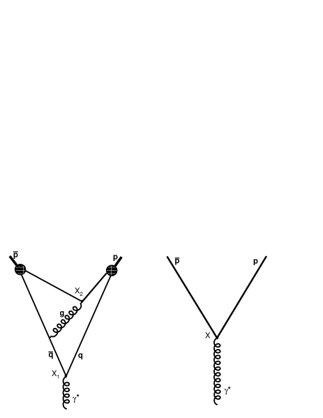
Fig. 4: Left image: one of the possible chains of events that at resolved level lead to proton-antiproton formation from a virtual photon. In this figure the proton is schematized in a simplified form, as composed by a charged quark plus a neutral compact diquark. So $\gamma$ $\rightarrow$ $\bar{p}p$ requires at least 2 pair creation vertexes, in the four-points $X_{1}$ and $X_{2}$. Right image: the same process at unresolved level of analysis. Only one vertex is present in the four-point $X$, where the $\bar{p}p$ pair is directly created by the photon. The relation between $X$, $X_{1}$, and $X_{2}$ is determined by Eq. (33), that in this simple case will be of the form $X$ $=$ $w_{1}X_{1}$ $+$ $w_{2}X_{2}$. The corresponding geometry is represented in Fig. 5.

With more than one charged quark in a Fock state of $N$ constituents, $F(q)$ is at first order a sum over all the amplitudes where the photon directly interacts with one of these charges, so that in one amplitude $x$ $=$ $x_{1}$, in another one $x$ $=$ $x_{2}$ and so on. In addition, we must sum over Fock configurations involving different numbers of constituent partons or even intermediate state hadrons.

These details concern the model one is applying, but in any case the structure suggested by Eqs. (33,38) will be present. We will find a four-coordinate $X$ representing the point where the photon creates the $unresolved$ proton-antiproton pair. This coordinate leads to the momentum-conserving $\delta^{4}$ function, and has no other role. Indeed, being $e^{iq_{\mu}X^{\mu}}$ the wave function of the photon, all the spacetime points are perfectly equivalent for this creation. The coordinate separation and the introduction of relative coordinates in Eq. (34) implies that the form factor is calculated by implicitly assuming that the unresolved proton-antiproton pair is created in the origin.

At resolved level, in the diagram where the i-th quark-antiquark pair is the active pair directly created by the photon, the argument $x$ of the form factor is the four-position $x_{i}$ of this pair creation with respect to the origin.

Let us again consider for simplicity the case where only the quark-antiquark pair “1” is charged. $R(t)$ is an integral of the form $\int d^{3}\vec{x}\int d^{4}x_{2}...$. In a model for $e^{+}e^{-}$ $\rightarrow$ $\bar{p}p$ where all the events $x_{2}$, $x_{3}$, … are causally consequent to the first pair creation in $x$ $=$ $x_{1}$, all the four-points $x_{2}$, $x_{3}$ …. must be in the future light cone of $x$, and $t$ $=$ $t_{1}$ is the most negative of all the involved times $t_{1}$, $t_{2}$… $t_{N}$. Because the origin is an average of all the $x_{i}$ with positive coefficients $w_{i}$, the origin is in the future light cone of $x$ $\equiv$ $x_{1}$. So $t$ is negative, and $x$ $=$ $(t,\vec{x})$ is in the past light cone of the origin. In the reverse process $\bar{p}p$ $\rightarrow$ $\gamma^{*}$, the same logic implies $t$ $>$ 0, and $x$ is in the future light cone of the origin.

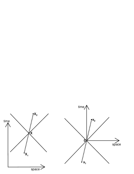
Fig. 5: Absolute (left image) and relative (right image) coordinates for the chain of events leading to $\bar{p}p$ formation from a virtual photon as shown in Fig. 4. Left image: according to Eqs. (33), $X_{1}$, $X$ and $X_{2}$ lie along a straight line, that is represented as a thick dashed line in the figure. This line does not correspond to any physical particle, we just use it to highlight the relative position of the three points. The continuous thin straight lines at 45^o and 135^o represent the light cone of $X$. Right image: the same geometry of the left image, but using the relative four-coordinates $x_{1}$ and $x_{2}$ introduced in Eqs. 34. With this transformation, $X$ becomes the origin. The four-coordinate $x$ that is argument of the space-time form factor $F(x)$ coincides with $x_{1}$, the four-point where the photon creates the first quark-antiquark pair.

The previous Eqs. (36-38) could be repeated for the SLFF. In this case however, $x$ would not lie in the (past or future) light cone of the origin. This means that although $\Phi^{+}(x_{1},x_{2},...)$ may represent a final proton with the same four-momentum in both the SL and the TL cases, the identity between $\Phi_{SL}^{+}(x_{1},x_{2},...)$ and $\Phi_{TL}^{+}(x_{1},x_{2},...)$ must be meant in analytic continuation sense. Measures in the SL sector produce a knowledge on $\Phi(...)$ that requires an extrapolation, to be applied to the TL sector. The same must apply to $F(x)$.

V Examples

The simplest examples approximate the proton as “single charged active quark plus neutral spectator diquark”. As above indicated, let the origin $X=(0,0,0,0)$ be the four-point where the unresolved $\bar{p}p$ pair is created. Let $(t_{1},\vec{x}_{1})$ be the point where the initial active quark-antiquark pair is created, and $(t_{2},\vec{x}_{2})$ the point where the spectator-antispectator pair is created. Then, following Eq. (34), we have

$$x\ \equiv\ x_{1}\ =\ (x_{1}-x_{2})w,\hskip 14.22636ptw\ >\ 0.$$ (39)

For example, in the symmetric case we have $x_{1}=-x_{2}$ and $x=(x_{1}-x_{2})/2$. In general, $w$ may depend on parton masses and dynamics. Here the only relevant things are the following:

Causality implies that $t_{1}<t_{2}$, and since the weight coefficient $w$ is positive the origin is somewhere on the straight line joining $x_{1}$ and $x_{2}$. Since $x_{2}$ is in the future light cone of $x_{1}$, the origin is in the future light cone of $x=x_{1}$, and $t<0$.

In the initial examples we violate T-symmetry assuming that $F(x)$ is nonzero only for negative times (that describes proton-antiproton creation but not annihilation). Next we add the reverse process piece.

V.1 Case 1. Homogeneous distribution for positive times

We assume that after the initial quark-antiquark creation, the creation of the complete proton-antiproton system is possible at any time with equal probability if this happens inside the future light-cone of the first event. We don’t know how this probability is spatially distributed, but the integral over all the space is time-independent and we fix it to 1 at any given time. Since the unresolved $\bar{p}p$ pair is created for $t=0$, the condition ”$\bar{q}q$ pair created before $\bar{p}p$ pair” just means $t<0$.

$$R(t)\ =\ \theta(-t),$$ (40)

$$F(q)\ =\ \int e^{iqt}\theta(-t)\ =\ {\pi\over{\epsilon-iq}},$$ (41)

with infinitesimal $\epsilon$.

V.2 Case 2. Exponential damping

Common sense suggests that either the spectator pair and the complete proton-antiproton system are created soon after the active pair, or the process will lead to independent fragmentation of the initial quark and antiquark. So it is more realistic to generalize Eq. (40 ) to

$$R(t)\ =\ \theta(-t)e^{-a|t|}.$$ (42)

that suppresses the probability of the creation of an exclusive hadron pair for $|t|\gtrsim 1/a$. This leads to

$$F(q)\ =\ {\pi\over{a-iq}}\ =\ {{a\pi}\over{a^{2}+q^{2}}}+i{{q\pi}\over{a^{2}+q^{2}}},$$ (43)

where the difference with respect to the previous case is that $a$ is finite.

V.3 Case 3. Monopole-like shape

As observed in a previous section, $F(x)$ must be nonzero both in the future and in the past light-cone, to describe both $\bar{p}p$ creation or annihilation. These terms should be time-symmetric, apart for a possible phase difference. We sum two terms like the previous one, corresponding to positive and negative $t$. Taking them with the same phase, we get a monopole-like distribution, with the correct asymptotic of the form factor of a two-constituent hadron:

$$R(t)\ =\ \theta(t)e^{-at}\ +\ \theta(-t)e^{at}\ =\ e^{-a|t|}$$ (44)

$$F(q)/\pi\ =\ {1\over{a-iq}}\ +\ {1\over{a+iq}}\ =\ {{2a}\over{a^{2}+q^{2}}}.$$ (45)

The $1/a$ parameter has the meaning of a formation time. In this simple two-constituent model of the proton, we have two meaningful pair creation vertexes at times $T_{1}$ and $T_{2}$. This implies one relative time $t$, that according to Eqs. (33,35) has the magnitude of $t_{1}-t_{2}$ (for example, in a symmetric model $t=(t_{1}-t_{2})/2$). For $|t|\gg 1/a$, $R(t)$ is very small. This means that either the second pair is formed within $1/a$, or the initial pair will produce two separate hadron showers.

When $q\approx$ some quarkonium mass, the scale of this time may expand to the time life of a resonance: the initial pair may form a long-lived state, and the second pair has more time to be formed. This is discussed in detail below. As it is, Eq. (45) corresponds to a zero-mass resonance of width $a$.

The above monopole form with its $R(t)$ counterpart contains two properties of general character: (a) a correct $1/q^{2}$ asymptotic for the formation of a hadron pair when each hadron is formed by 2 constituents, (b) the presence of a time cutoff $1/a$, meaning that the formation of the full hadron pair and of the first quark-antiquark pair cannot be too far in time.

V.4 Case 4. Resonance-like, space and time parameters

Eq. (45) may be written as

$$F(q)/\pi\ =\ i\Big{(}{1\over{q+ia}}\ -\ {1\over{q-ia}}\Big{)}.$$ (46)

The $simplest$ way to have poles with nonzero mass is to substitute $q\to q-M$ leading to a Lorentzian (not Breit-Wigner) resonance shape:

$$F(q)/\pi\ =\ i\Big{(}{1\over{q-M+ia}}\ -\ {1\over{q-M-ia}}\Big{)}\ \propto\ {1\over{(q-M)^{2}}+a^{2}}.$$ (47)

This shape describes, for example, the stationary response of a classical damped oscillator to an external periodic force. By Fourier transform we get

$$R(t)\ \propto\ \ e^{iMt}\ e^{-a|t|}$$ (48)

Since a Fourier transform is a sum with homogeneous weight over all the frequencies, the previous $R(t)$ is the response of a classic damped oscillator to an instantaneous external force of the form $\delta(t)$ (Eqs. (47, 48) are the frequency and time Green functions of that problem).

Although a classical oscillator presents several similarities with some quantum systems, it has not the problem of the negative-energy solutions of the relativistic wave equation. We should remind that here $q$ means $q_{0}$ (the time component of the 4-vector $q_{\mu}$) and not $\sqrt{q^{2}}$, so it may be negative (we are in the CM frame where $\vec{q}=0$). Because of the relativistic particle-antiparticle symmetry, to each pole with $q_{0}=M+ia$ corresponds a pole with $q_{0}=-(M+ia)$ that describes the corresponding negative-energy states. With only positive $Re(q_{0})$ poles, we are back to the situation of the first two examples of this section, where $F(q)$ describes the $\bar{p}p$ creation process, but not the annihilation one. Indeed, by closing the integration path on the upper or lower half of the complex plane the Fourier transform returns us an $R(t)$ containing $\theta(\pm t)$. The two poles must be exactly opposite, so that the situation is unchanged if the physical photon energy $q_{0}^{\prime}=-q_{0}$ of the $\bar{p}p$ annihilation channel is used instead of $q_{0}$ to describe the amplitude.

A Breit-Wigner $probability$ distribution contains all the four poles $q_{0}$ $=$ $\pm(M\pm ia)$. The corresponding amplitude is

$$F_{\pm}(q)\ \propto\ {1\over{(q^{2}-M^{2})}\pm iMa}$$ (49)

where we may imagine several combinations of $F_{\pm}(q)$ composing a form factor. For example

$$F(q)\ \propto\ F_{+}(q)+F_{-}(q)$$ (50)

corresponds to

$$R(t)\ \propto\ \ cos(Mt)\ e^{-a|t|}.$$ (51)

and gives $F(q)=O(1/q^{2})$ at large $q$, as expected for the two-constituent hadron we are working with.

$F_{+}(q)$ and $F_{-}(q)$ contain respectively one pole from the the $\bar{p}p$ creation and one pole from the $\bar{p}p$ annihilation process. With arguments similar to those following Eq. (48), we may say that Eq. (51) sums two contributions, that may be highlighted by writing (see Fig.6)

$$R(t)\ \equiv\ R_{creation}(t)\theta(-t)\ +\ R_{ann}(t)\theta(t).$$ (52)

One of the two pieces describes the process in the $\bar{p}p$ creation channel, and it has the same form as the retarded response of a classical bound and damped oscillating system to a $\delta(t)$-shaped external perturbation. The other one has the same meaning, in the $\bar{p}p$ annihilation channel. Analytically, it may be also read as an unphysical advanced response in the creation process.

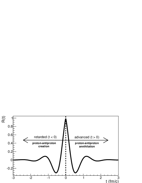
Fig. 6: $R(t)=\cos(Mt)e^{-a|t|}$, with $M=1$ GeV, $a=0.4$ GeV, as in Eq. (51). The retarded ($\bar{p}p$ creation) and advanced (annihilation) contributions of Eq. (52) are distinguished.

We know that the tail of a resonance may be much more complicated than this, and pole-based models of FFs Bijker and Iachello (2004); Belushkin et al. (2007); Iachello and Wan (2004) are more sophisticated than the above Lorentz and BW examples. However, the BW example contains the basics to remark a few points. First, $two$ dimensional and scaling-violating parameters appear, corresponding to the pole mass and width. For obvious reasons, in the SL analytic continuation $q^{2}\to-q^{2}$ the leading parameter expressing how a charge distribution decreases with the distance is the pole mass. In the TL case this mass is associated with the frequency of the oscillation in time of the underlying photon-quark-antiquark coupling. The parameter that tells us how fast is the decrease in time of the probability of the formation of the hadron pair is the pole width. Taking into account that fast-decaying hadron resonances have mass $\sim$ 1 GeV, and standard width in the range 0.1-1 GeV, we expect for $R(t)$ a shape like in Fig. 6, with a small number of visible oscillations. If the pole had zero width the oscillation would continue forever, like in the first example of this section where $a$ was infinitesimal leading to $R(t)$ $=$ $\theta(t)$. This would not prevent from having a finite charge radius in the SL measurement given by $<r>\sim 1/M$. The SLFF would appear as a monopole $1/(|q^{2}|+M^{2})$.

V.5 Case 5. Several spectators: dipole and asymptotic $1/q^{2(n-1)}$ behavior

A nucleon is made of three constituents in its basic valence state, possibly more in temporary fluctuations. Because of the valence structure, for the nucleon FF we expect a $1/q^{4}$ law at large $q$, and more in general a $1/q^{2(n-1)}$ law if the produced hadrons are made of $n$ compact constituents. Since this behavior does not depend on the relative wave function or interaction of these constituents, we would like to identify a mechanism that leads to the correct asymptotic form, whichever these details may be.

We may use the Fourier transform property of convolutions:

$$F_{1}(q)F_{2}(q)\ =\ F.T.\Big{[}R_{1}(t)*R_{2}(t)\Big{]},$$ (53)

where

$$\Big{[}R_{1}(t)*R_{2}(t)\Big{]}\ \equiv\ \int d\tau R_{1}(\tau)R_{2}(t-\tau).$$ (54)

So a function like

$$F(q)\ \propto\ {1\over{(a^{2}+q^{2})(b^{2}+q^{2})}},$$ (55)

that presents the required asymptotic trend, is the Fourier transform of

$$R(t)\ =\ \int d\tau\ e^{-a|t-\tau|}\ e^{-b|\tau|}.$$ (56)

This contains the required statistical properties. In a three-constituent Fock state the proton has two internal (four-dimensional) degrees of freedom. One of the two convoluted terms has the same role and meaning it had in the previous two-constituent case, and is associated to the degree of freedom that is directly probed by the virtual photon. The other term represents a decaying correlation between the active and a spectator degree of freedom. Being dominated by simple valence configurations, the large-$q$ behavior will derive from a sum of three terms like Eq. (56). In each term one of the three valence quarks plays the role of active quark.

In Fig. 7 we show an example of convolution with $R_{1}(t)$ and $R_{2}(t)$ of resonance type (see Eq. (51)). The final shape depends (even at qualitative level) on the parameters of the convoluting $R_{1}$ and $R_{2}$, but some rules are simple: If the decay times of $R_{1}$ and $R_{2}$ are different, $R_{1}*R_{2}$ coincides at large $|t|$ with the one between $R_{1}$ and $R_{2}$ with the longer lifetime. $R_{1}*R_{2}$ may decay for two reasons: (a) because the oscillations of $\cos(M_{1}t)$ and $\cos(M_{2}t)$ acquire opposite phase (for $t\approx\pi/(M_{1}-M_{2})$), (b) because $t>1/a_{long}$, where “long” refers to the longer-life pole. So the decay time of the convolution is determined by the largest between $|M_{1}-M_{2}|$ and the width of the longer-life pole. If the process is dominated by standard hadron poles like $\rho$, $\omega$ the decay time is of magnitude 1/(200 MeV) $\sim$ 1 fm. Narrow large-mass poles could lead to much more unpredictable effects. Since the poles entering the convolution are poles of quark-antiquark states, they can also be poles of the full proton-antiproton system.

The dynamical meaning of the convolution in Fig. 7 is described in Fig. 8. As observed after Eqs. (48) and (52), $R(t)$, when derived from a Lorentz or Breit-Wigner form, corresponds to the response of a classical damped oscillator to a $\delta(t)$ external perturbation. The convolution structures of Eq. (54) describe the response of a chain of two oscillators, where one end of the chain is directly under the strain of the virtual photon.

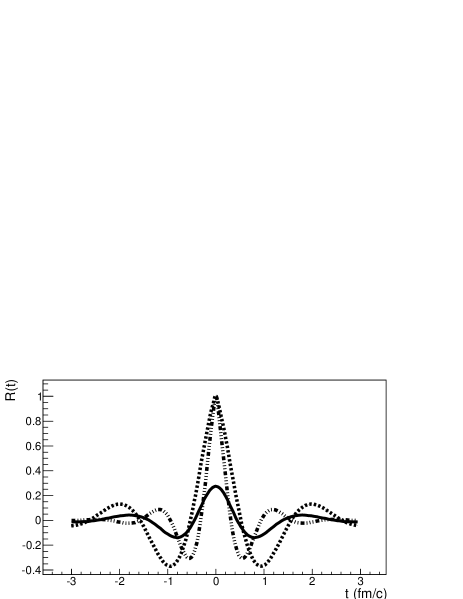
Fig. 7: Dotted line: $R_{1}(t)=\cos(M_{1}t)e^{-a|t|}$, with $M=1$ GeV, $a=0.4$ GeV; thick-soft double-dotted line: $R_{2}(t)=\cos(M_{2}t)e^{-b|t|}$, with $M_{2}=0.6$ GeV, $b=0.1$ GeV; continuous line: convolution $[R_{1}(t)*R_{2}(t)]=\int d\tau R_{1}(\tau)R_{2}(t-\tau)$ according to Eq. (54).

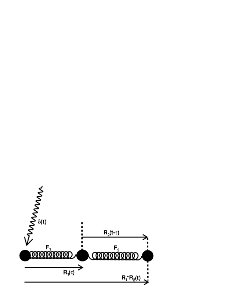
Fig. 8: Sequence of oscillators corresponding to the response function of Fig. 7. In equilibrium both the black masses overlap with the grey circle. They can move horizontally under the action of elastic forces $F_{1}$ and $F_{2}$, graphically represented as springs, or of external forces. When any of these masses is subject to an instantaneous external impulse $\propto$ $\delta(t-t_{0})$ at the time $t_{0}$, its later displacement from the equilibrium position is described by the Green response function $R_{i}(t-t_{0})$. A short impulse by an external force $\delta(t)$ at $t=0$ causes the displacement $R_{1}(\tau)$ of the first mass at the later time $\tau$. The displacement of the first mass acts as an external force on the second mass, and may be decomposed into short impulses: $R_{1}(\tau)=\int d\tau^{\prime}R_{1}(\tau^{\prime})\delta(\tau-\tau^{\prime})$. Since each short impulse at the time $\tau$ produces a response $R_{2}(t-\tau)$ of the second mass, the resulting displacement of the second mass is $\int d\tau R_{2}(t-\tau)R_{1}(\tau)$.

In sub-asymptotic conditions more degrees of freedom could play a role. These terms would imply a longer chain of convolutions. For example, with four constituents we would have

$$R(t)\ =\ \Big{[}[R_{1}(t)*R_{2}(t)]*R_{3}(t)\Big{]}$$ (57)

leading to a form factor that empirically could appear as a product of monopoles

$$F(q)\ \propto\ {1\over{(q^{2}\pm a^{2})(q^{2}\pm b^{2})(q^{2}\pm c^{2})}}.$$ (58)

where the sign (in the TL channel) is negative if the mass is larger than the width of a pole, positive in the opposite case. A three-pole structure would be found in a process like $e^{+}e^{-}\rightarrow\bar{p}n\pi^{+}\rightarrow\bar{p}p$ where three quark-antiquark creation vertexes $x_{1}$, $x_{2}$, $x_{3}$ are needed to create the intermediate state. For example, the data from the BABAR collaboration Lees et al. (2013a, b) are well fitted by Eq. (5) that has the sub-asymptotic form $F(q)\propto 1/(q^{2}+a^{2})(q^{2}-b^{2})^{2}$.

V.6 Case 6. Oscillating modulations, and delayed or advanced terms

If we have the sum of two contributions of equal shape

$$R(t)\ = \ R_{0}(t)\ +aR_{0}(t-b),\ a\ll 1,$$ (59)

$$F(q)\ = \ F_{0}(q)[1+ae^{ibq}],$$ (60)

because of a known property of the Fourier transforms: $F.T.[G(t-b)]=e^{iqb}F.T.[G(t)]$.

We expect a similar phenomenon if the second distribution is not exactly identical to the first one, but is similar. For example, $R_{0}(t)$ could have a peak in $T$, and $R_{1}(t)$ a similar peak in $T-b$. This would lead to a periodic modulation.

The oscillating modulation discussed in Bianconi and Tomasi-Gustafsson (2015, 2016) however, shows a periodic pattern with respect to the final state hadron relative momentum, rather than to $q$. So, that phenomenon requires a more complex explanation, where the role of the final state kinematics is more explicit.

VI Conclusions

We have explored a scheme where the TL hadron FF is interpreted as an amplitude for the distribution in time of the quark-antiquark pair creation vertex. This is the timelike counterpart of the known interpretation of the spacelike form factor as the Fourier transform of a classical charge distribution.

Exploiting analytic continuity between the physical reactions where both FFs are measured, these are considered to be the analytic continuation of a unique function $F(q)$. For real values of the components of $q_{\mu}$, $F(q)$ is assumed to be the four-dimensional Fourier transform of a unique function $F(x)$, that is $F(q)\equiv\int e^{iq_{\mu}x^{\mu}}F(x)$.

Giving to $q_{\mu}$ the spacelike and timelike components $(0,\vec{q})$ and $(q,0)$, we get $F_{SL}(q)=\int d^{3}\vec{x}\rho(\vec{x})$, and $F_{TL}(q)=\int dtR(t)$, where $\rho(\vec{x})=\int dtF(x)$, and $R(t)=\int d^{3}\vec{x}F(x)$. So the distributions that are tested by the virtual photon wave are projections onto orthogonal one-dimensional and three-dimensional spaces of the same underlying function $F(x)$.

We have next explored the main properties of the function $F(x)$. The contributions to the timelike form factor appearing in the reactions of proton-antiproton creation and annihilation originate from those $x$ that lie in the future and past light cones of the origin. The former contributes to the $e^{+}e^{-}\rightarrow\bar{p}p$ reaction, the latter to the reverse process. A phase asymmetry between the values of $F(x)$ in the two light cones is allowed by general invariance rules. This in principle permits an imaginary part to be present in $F(q)$ even if $F(x)$ is real.

Next we have presented some simple examples for possible $R(t)$ functions with consequent form factors. These were not models, but rather the simplest possible functions presenting realistic phenomenological features: a dimensional parameter associated with the hadron pair formation time, the expected large $q$ power counting behavior, and interference phenomena.

In conclusion, the present interpretation of FFs in the time-like region highlights the spacetime meaning of these fundamental quantities, and relates the static charge density features with the time evolution properties of the hadron pair formation.

This interpretation will help understanding high precision data expected to come from future measurements. Experimental programs at all existing and planned hadron facilities are on going or foreseen, for example at Mainz (Germany), JLab (USA) in the SL region, and, in the TL region, at VEPPII (Russia), BESIII at BEPC2 (China) and at the future antiproton facility PANDA at FAIR (Germany).

References

- Zichichi et al. (1962) A. Zichichi, S. Berman, N. Cabibbo, and R. Gatto, Nuovo Cim. 24, 170 (1962).
- Pacetti et al. (2015) S. Pacetti, R. Baldini Ferroli, and E. Tomasi-Gustafsson, Phys.Rep. 550-551, 1 (2015).
- Denig and Salme (2013) A. Denig and G. Salme, Prog.Part.Nucl.Phys. 68, 113 (2013).
- Bardin et al. (1994) G. Bardin, G. Burgun, R. Calabrese, G. Capon, R. Carlin, et al., Nucl.Phys. B411, 3 (1994).
- Lees et al. (2013a) J. Lees et al. (BaBar Collaboration), Phys.Rev. D87, 092005 (2013a).
- Lees et al. (2013b) J. Lees et al. (BaBar), Phys.Rev. D88, 072009 (2013b).
- Ablikim et al. (2015) M. Ablikim et al. (BESIII Collaboration), Phys. Rev. D 91, 112004 (2015).
- Ablikim et al. (2005) M. Ablikim et al. (BES Collaboration), Phys.Lett. B630, 14 (2005).
- Bianconi and Tomasi-Gustafsson (2015) A. Bianconi and E. Tomasi-Gustafsson, Phys. Rev. Lett. 114, 232301 (2015).
- Bianconi and Tomasi-Gustafsson (2016) A. Bianconi and E. Tomasi-Gustafsson, Phys.Rev.C 93, 035201 (2016).
- Ambrogiani et al. (1999) M. Ambrogiani et al. (E835 Collaboration), Phys.Rev. D60, 032002 (1999).
- Lepage and Brodsky (1979) G. P. Lepage and S. J. Brodsky, Phys.Rev.Lett. 43, 545 (1979).
- Shirkov and Solovtsov (1997) D.V. Shirkov and I.L. Solovtsov, Phys.Rev.Lett. 79, 1209 (1997).
- Kuraev (2008) E. A. Kuraev, Private communication (2008).
- Brodsky and de Teramond (2008) S. J. Brodsky and G. F. de Teramond, Phys.Rev. D77, 056007 (2008).
- Tomasi-Gustafsson and Rekalo (2001) E. Tomasi-Gustafsson and M. Rekalo, Phys.Lett. B504, 291 (2001).
- Ablikim et al. (2010) M. Ablikim et al. (BESIII Collaboration), Chin. Phys. C34, 421 (2010).
- Pakhlova et al. (2008) G. Pakhlova et al. (Belle), Phys. Rev. Lett. 101, 172001 (2008).
- Ablikim et al. (2006) M. Ablikim et al. (BES), Phys. Rev. Lett. 96, 162002 (2006).
- Ablikim et al. (2004) M. Ablikim et al. (BES), Phys. Rev. Lett. 93, 112002 (2004).
- Bai et al. (2003) J. Z. Bai et al. (BES), Phys. Rev. Lett. 91, 022001 (2003).
- Amsler et al. (1994) C. Amsler et al. (Crystal Barrel), Phys. Lett. B340, 259 (1994).
- Matveev et al. (1973) V. Matveev, R. Muradyan, and A. Tavkhelidze, Teor.Mat.Fiz. 15, 332 (1973).
- Brodsky and Farrar (1973) S. J. Brodsky and G. R. Farrar, Phys.Rev.Lett. 31, 1153 (1973).
- Gousset and Pire (1995) T. Gousset and B. Pire, Phys. Rev. D51, 15 (1995).
- Bijker and Iachello (2004) R. Bijker and F. Iachello, Phys.Rev. C69, 068201 (2004).
- Adamuscin et al. (2005) C. Adamuscin, S. Dubnicka, A. Dubnickova, and P. Weisenpacher, Prog.Part.Nucl.Phys. 55, 228 (2005).
- Belushkin et al. (2007) M.A. Belushkin, H.-W. Hammer, and Ulf-G. Meissner, Phys.Rev. C75, 035202 (2007).
- Lomon and Pacetti (2012) E. L. Lomon and S. Pacetti, Phys.Rev. D85, 113004 (2012), eprint 1201.6126.
- Bianconi et al. (2006a) A. Bianconi, B. Pasquini, and M. Radici, Phys. Rev. D74, 034009 (2006a).
- Bianconi et al. (2006b) A. Bianconi, B. Pasquini, and M. Radici, Phys. Rev. D74, 074012 (2006b).
- Gakh and Tomasi-Gustafsson (2005) G. Gakh and E. Tomasi-Gustafsson, Nucl.Phys. A761, 120 (2005).
- Gakh and Tomasi-Gustafsson (2006) G. Gakh and E. Tomasi-Gustafsson, Nucl.Phys. A771, 169 (2006).
- de Melo et al. (2004) J. de Melo, T. Frederico, E. Pace, and G. Salme, Phys.Lett. B581, 75 (2004).
- de Melo et al. (2006) J. P. B. C. de Melo, T. Frederico, E. Pace, and G. Salme, Phys. Rev. D73, 074013 (2006).
- Kuraev et al. (2012) E. Kuraev, E. Tomasi-Gustafsson, and A. Dbeyssi, Phys.Lett. B712, 240 (2012).
- Lorenz et al. (2015) I. T. Lorenz, H.-W. Hammer, and Ulf-G. Meissner, Phys. Rev. D 92, 034018 (2015).
- Haidenbauer et al. (2014) J. Haidenbauer, X.-W. Kang, and Ulf-G. Meissner, Nuclear Physics A 929, 102 (2014).
- Baldini et al. (2009) R. Baldini, S. Pacetti, A. Zallo, and A. Zichichi, Eur. Phys. J. A39, 315 (2009).
- Bianconi et al. (2014) A. Bianconi, E. Lodi Rizzini, V. Mascagna, and L. Venturelli, Eur. Phys. J. A50, 182 (2014).
- Zimmer et al. (2012) O. Zimmer, C. A. Dominguez, H. Falomir, and M. Loewe, Phys. Rev. D85, 013004 (2012).
- Iachello and Wan (2004) F. Iachello and Q. Wan, Phys.Rev. C69, 055204 (2004).